Abstract
In this paper, we develop the explicit finite difference method (FDM) to solve an ill-posed Cauchy problem for the 3D acoustic wave equation in a time domain with the data on a part of the boundary given (continuation problem) in a cube. FDM is one of the numerical methods used to compute the solutions of hyperbolic partial differential equations (PDEs) by discretizing the given domain into a finite number of regions and a consequent reduction in given PDEs into a system of linear algebraic equations (SLAE). We present a theory, and through Matlab Version: 9.14.0.2286388 (R2023a), we find an efficient solution of a dense system of equations by implementing the numerical solution of this approach using several iterative techniques. We extend the formulation of the Jacobi, Gauss–Seidel, and successive over-relaxation (SOR) iterative methods in solving the linear system for computational efficiency and for the properties of the convergence of the proposed method. Numerical experiments are conducted, and we compare the analytical solution and numerical solution for different time phenomena.
Keywords:
continuation problem; inverse and ill-posed problem; acoustic wave equation; numerical analysis; regularization; finite difference method MSC:
35R30; 65M30; 65F10; 80M20
1. Introduction
For hyperbolic differential equations, problems with Cauchy data on non-spatial surfaces began to be studied by F. John (1960, 1961 [1,2]).
In the study of many practical problems, the Cauchy problem for hyperbolic equations occurs, and the Cauchy problem for the acoustic wave equation has been investigated in many works by Douglas (1960, [3]) and Cannon (1964, 1965 [4,5]).
According to Hadamard [6,7], the solution to the Cauchy problem for an acoustic wave equation is ill-posed, and it exists when we impose smoothness conditions or strong compatibility on the initial data. Hadamard showed that a global solution cannot exist unless a certain compatibility relation is established among the Cauchy data. Further, he showed that even if the data are such, a classical solution exists, and it does not continuously depend on the data. According to Hadamard, these problems are well known to be ill-posed, and from various aspects, many investigations have been attempted, such as regularization, existence–uniqueness theorems, and least squares methods by Payne (1975, [8]), for such problems have been discussed. The problem and its applications were then investigated in [9,10,11,12,13,14,15,16,17].
Inverse and ill-posed problems for three-dimensional acoustic waves in the time domain have been studied theoretically with a number of methods of different hyperbolic equations [16,18,19,20]: hyperbolic systems [21], the Green function approach, and wave splitting [22,23].
The method of scales and the Banach spaces of analytic functions were developed in some of the variables to study the Cauchy problem, and used to solve the inverse problem of determining the potential in the hyperbolic equation by V. Romanov (1996, [24,25]).
Helsing et al. (2011, [26]) rewrote the Cauchy problem as an operator equation using the Dirichlet-to-Neumann map on the boundary.
The singular values of the operator of continuation problems were investigated, and a comparative analysis of numerical methods was presented [27,28,29,30].
To model wave propagation in medicine, geophysics, and engineering, among others [31], the acoustic wave equation has been widely used with a non-zero point source function. Imaging these waves in the field of medicine was shown to provide very objective information about the biological tissue being examined. Acoustic wave equations arise widely in various applications such as seabed exploration and underground imaging.
Causon et al. (2010, [32]) provided an introduction to the finite difference method (FDM) to solve partial differential equations (PDEs) and the theory of Jacobi, Gauss–Seidel, and successive over-relaxation (SOR) iterative solution methods.
Due to simple implementation and high accuracy, finite difference methods have attracted great interest from many researchers from various areas of science and engineering over the past several decades. Alford et al. (1974, [33]), Tam et al. (1993, [34]), and Yang et al. (2012, [35]) introduced many FDMs that have been developed to solve the acoustic wave equations.
The FDM is a powerful tool for acoustic or seismic wave simulations due to its high accuracy, low memory, and fast computing speed, especially for models with complex geological structures studied by Liao et al. (2011, [36]), Finkelstein et al. (2017, [37]), and Zapata et al. (2018, [38]).
Alexandre et al. (2014, [39]) studied an explicit finite difference method to solve the acoustic wave equation using locally adjustable time steps; by considering stability, the time step size is initially determined by the medium with higher wave speed propagation, resulting in the fact that, in the whole domain, the higher the speed, the lower the time step needs to be to ensure stability.
Liu et al. (2009, 2010, [40,41,42]) and Liang et al. (2013, [43]) investigated the numerical solution of acoustics with a vertical axis of symmetry (VTI) modeling and a new time–space domain dispersion relation-based finite difference scheme of the acoustic wave equation and an implicit staggered grid finite difference method for seismic modeling, which plays an important role in seismic wave propagation, seismic imaging, and full waveform inversion.
Liao et al. (2018, [44]) proposed a compact high-order FDM using a novel algebraic manipulation of finite difference operators for 2D acoustic wave equations with variable velocity.
Young (1971, [45]) found an iterative solution of large linear systems using the SOR iterative method. Dancis (1991, [46]) used the SOR iteration method to solve linear equations of large sparse systems and to approximate many of the PDEs that arise in engineering and showed that, using a polynomial acceleration together with a suboptimal relaxation factor, a smaller average spectral radius can be achieved.
Rigal (1979, [47]) applied the successive over-relaxation method to non-symmetric linear systems to give the convergence domain of this method with the SOR algorithm to find the best relaxation factor in this domain.
Hadjidimos (2000, [48]) studied the theory of SOR method and some of its properties and mentioned the role of SOR and symmetric SOR methods as preconditioners for the class of semi-iterative methods.
Britt et al. (2018, [49]) introduced an energy method to derive the stability condition for the variable coefficient case using a finite difference scheme of high-order compact time–space for the wave equation.
Additionally, we can see some generalized finite difference schemes, for example, in [50], incompressible two-phase fluid flows, i.e., a conservative Allen–Cahn–Navier–Stokes system solved using a new numerical scheme based on the first-order time-splitting approach, and it has been applied to deal with the time variable.
Qu et al. (2018, [51]) solved the inhomogeneous modified Helmholtz equation using Krylov-deferred correction (KDC) and generalized FDM for a highly accurate solution of transient heat conduction problems; in [52], a hybrid numerical method for 3D heat conduction in functionally graded materials is developed that integrates the advantages of general FDM and KDC techniques.
Belonosov et al. (2019, [53]) solved the continuation problem for the 1D parabolic equation with the data given on the boundary part through comparative analysis of numerical methods.
Chung et al. (2021, [54]) investigated a least squares formulation for inverse ill-posed problems. The existence and uniqueness of an inverse solution and the continuity of the inverse solution were established for noisy data in .
Desiderio et al. (2023, [55]) solved the 2D time-domain damped wave equation using a boundary element method (BEM) and a curved virtual element method (CVEM) for the simulation of scattered wave fields by obstacles immersed in infinite homogeneous media.
Bzeih et al. (2023, [56]) studied the 2D linear wave equation with dynamical control on the boundary using the finite element method.
The backward parabolic problem was investigated [57], and the error estimates of the method were proved with respect to the noise levels.
Using a space–time discontinuous Galerkin method, the unique continuation problem was solved for the heat equation by Burman et al. (2023, [58]), and the consistency error and discrete inf-sup stability were established, and it led to a priori estimates on the residual.
Dahmen et al. (2023, [59]) solved ill-posed PDEs that are conditionally stable concerning the design and analysis of least squares solvers, and in view of the conditional stability assumption, a general error bound was established.
Helin (2024, [60]) studied the statistical inverse learning theory with the classical regularization strategy of applying finite-dimensional projections and derived probabilistic convergence rates for the reconstruction error of the estimator of maximum likelihood (ML).
Epperly (2024, [61]) solved overdetermined linear least squares problems using iterative sketching and sketch-and-precondition randomized algorithms and showed that, for large problem instances, iterative sketching is stable and faster than QR-based solvers.
Qu et al. (2024, [62]) introduced a numerical framework with stability over long time intervals by addressing dynamic crack problems, spatial and temporal discretizations through the meshless generalized finite difference method, and the arbitrary order KDC method to numerically simulate the system of spatial PDEs generated at each time node.
Li (2025, [63]) proposed a novel iterative method, termed the Projected Newton method (PNT), to solve large-scale Bayesian linear inverse problems; this method can update the solution step and the regularization parameter simultaneously without decompositions and expensive matrix inversions.
Bakanov et al. (2025, [64]) proposed the Jacobi numerical method to solve the 3D continuation problem for a wave equation based on FDM.
In addition, for three-dimensional problems in the time domain, it usually results in sparse and large linear systems, so at each time step, that needs an iteration. In this work, we extend the formulation of the Jacobi, Gauss–Seidel, and SOR iterative methods to solve the linear systems. The conclusion of this study finds that all three iterative methods are accurate; however, the SOR iterative method is more efficient in terms of fewer iterations and fewer execution times and faster convergence compared with the other two iterative methods.
This paper is organized as follows: The three-dimensional acoustic wave equation in the time domain is formulated in Section 2. We give a problem formulation and an overview of the three different iterative schemes, followed by the convergence analysis. In Section 3, finite difference approximations can be described based on the seven-point centered formula that is applied to discretize the three-dimensional acoustic wave equation with difference schemes. Section 4 present the applicability of the proposed schemes by performing some numerical experiments. In Section 5, we discuss the results. Finally, we give our conclusions and remarks in Section 6.
2. Statement of the Problem
In this paper, we consider the three-dimensional hyperbolic acoustic wave equation.
2.1. Cauchy Problem (Continuation Problem)
Consider the ill-posed [65] continuation problem in which the unknown function satisfies the following boundary value problem (BVP) in the domain , as follows:
here, is a function of space and time and c is the propagation of the velocity of the medium wave, is a non-zero function that represents the wave velocity, and is a source function, together with initial conditions and and the aforementioned suitable boundary conditions.
Suppose that , , and are given functions and
2.2. Inverse Problem
We assume that the function is unknown. However, instead of , we have the following additional information concerning the solution of DP, as follows:
The inverse problem (IP) consists in finding the function from (1)–(5), (7), and (8).
The inverse problem in (1)–(5), (7), and (8) is equivalent to the continuation problem in (1)–(6) in the following sense. If we solve the continuation problem, then we can find , i.e., the solution of inverse problem q. Conversely, if we solve the inverse problem and find the solution of the inverse problem, we can set and solve the direct problem in (1)–(5), and (7) and find —the solution of the continuation problem.
2.3. Operator Form of the Inverse Problem
2.4. Linear Neural Network
Suppose that we have a system of sources g and receivers g.
We construct a linear neural network that maps
and obtain the mapping
therefore,
2.5. General Formulation of Continuation Problem
Let us consider the following continuation problem:
with the operator acting from to and having the form
2.6. Ill-Posedness
Its solution is unique, but it does not depend continuously on the Cauchy data. By the following example, the instability of the solution can be illustrated
it is easy to see that, for , the data tend toward zero, while the solution
increases indefinitely in an arbitrarily small neighborhood of .
2.7. Conditional Stability Estimate
2.8. Continuation Problem for the Helmholtz Equation
Let us investigate the stability of the continuation problem. We suppose and consider the continuation problem for the Helmholtz equation [66,67,68,69,70], as follows:
here,
is permeability, is conductivity, is frequency.
The continuation problem in (13)–(16) consists in finding the function in the domain , by the given boundary conditions (14)–(16).
Let us formulate the continuation problem in the form of an inverse problem. We introduce the following direct problem:
Inverse problem: find the function using additional information, as follows:
Let us find the solution to the direct problem in (17)–(19). We suppose that has the following form:
and will find the direct problem solution, as follows:
solving the sequence of direct problems, as follows:
here,
The general solution of Equation (21) has the following form:
here, , and
Therefore, the solution of the problem in (21), (22) is given by the following formula:
Then the direct problem solution in (17)–(19) is given by the following Fourier series:
therefore, the solution of the inverse problem in (17)–(20) is given by Fourier series expansion, as follows:
Thus, the singular values of the operator A have the following form:
Consider particular cases of singular values of the operator A.
- Laplace equation , :
- The parabolic equation ,
- The Helmholtz equation , :and .According to [71], on the wave number , the singular values depend strongly. The singular values of A are bounded below by 1 in the low-frequency domain , where the singular values decay exponentially for the high-frequency domain. In the low-frequency domain, the operator A is continuously invertible, and this domain increases with , which is the most important fact.
2.9. Limitations of Direct Methods
When the size of the coefficient matrix increases, the number of operations required increases rapidly to solve the equation sets. For large linear systems, direct methods are computationally very expensive. Usually, iterative methods are a preferred choice to solve large systems.
2.10. Iterative Methods
We use iterative methods to solve the system of linear equations that arise from the finite difference approximations of PDEs, which have large and sparse coefficient matrices. For the unknown vector q of , the process starts with an initial approximation, and by an iterative process, the successive approximations will be improved.
where and are the and approximations for the solution of the linear set of equations.
R is called the non-singular iteration matrix depending on A.
C is called the constant column vector.
Given , classical methods generate a sequence that converges to the solution , where is calculated from by iterating (23). The iterative method strategy generates a sequence of approximate solution vectors for the system . The process can be stopped when
in the limiting case, where converges to the exact solution . From (24), the exact solution q can be found, that is, a stationary point; if is equal to the exact solution of the set of equations, then will be equal to the exact solution.
2.11. Classical Iterative Methods
Based on [48], using the principle that the matrix A can be written as the sum of other matrices, classic iterative methods are built. There are many ways to divide the matrix; two of them are the origin of the Jacobi and the Gauss–Seidel method. The successive over-relaxation method is an improved version of the Gauss–Seidel method. Classic iterative methods generally have quite a low convergence rate.
The matrix A is split into two matrices, which are M and K such that . Here, M is a diagonal matrix with entries such as A on the main diagonal, the matrix K has zeros on the diagonal, and the off-diagonal entries are equal to the rest of the entries in A. By applying this to the set of linear equations, we obtain
where M is the preconditioner, or the preconditioning matrix is taken to be invertible and solve for q. We obtain
where and . Here, R is called an iteration matrix.
Definition 1
([45,72]). The matrix is an M-matrix if for all , A is non-singular, and . If A is irreducible and has a strict inequality at least on i, then A is an M-matrix.
We write (25) in the component form, which gives the following expression:
Lemma 1.
Let be any operator norm . Then, if converges for any .
Proof of Lemma 1.
The spectral radius of the matrix A, denoted by
where the maximum is taken from the overall eigenvalues of A.
Lemma 2
([73]). For all operator norms , .
Corollary 1.
The iteration converges to the solution for all initial and for all f if .
Proof of Corollary 1.
This corollary follows from Lemmas 1 and 2. □
Remark 1.
The measure of the number of iterations that are needed to converge to the given tolerance is the convergence rate of the iterative scheme , and it is defined as . This means that the smaller , the higher the rate of convergence. Therefore, the method is said to be efficient if we choose a splitting so that
1. and are easy to evaluate;
2. is small.
The splitting of the methods that we discussed in this section shares the following notation:
where D is the diagonal of the matrix A, L is the lower triangular part of the matrix A, and U is the upper triangular part of the matrix A.
2.11.1. Jacobi Iterative Method
All the entries in the current approximation will be updated on the basis of the values in the previous approximation in the Jacobi iterative method. The splitting of the coefficient matrix A for the Jacobi iterative method is , and its iteration gives the following result:
where
The component form of Equation (28) is (see [74,75])
where the initial guess for the solution can be arbitrarily chosen.
Always, we start with the zero initial vector . The Jacobi iteration starts with an initial approximation , and repeatedly applies the update of Jacobi to create a sequence that converges to the exact or analytical solution. With the control we apply for iteration to check the residual and compute iterate , the residual is defined by
and control error using Root Mean Square normalization (RMS norm) . However, if we do not know the true solution, the proper way to control and terminate an iteration is to monitor the residual.
The difference between the approximate solution (29) and the exact solution (26) is defined as an error, as follows:
each component of the error satisfies
where is the error at the approximation, so
where
This shows that the rate of convergence is linear. Equation (30) implies that
and so on
If , as , then as , the Jacobi iteration method converges.
Definition 2
([45]). The matrix A is said to be diagonally dominant if and only if . In order for to be true, the coefficient matrix A must be diagonally dominant, that is,
Therefore, if A is diagonally dominant and if the given system of linear equations is strictly diagonally dominant by rows, the Jacobi method converges.
2.11.2. Gauss–Seidel Iterative Method
The Gauss–Seidel method uses the values previously updated in the current approximation to find the rest. The splitting of the matrix A for the Gauss–Seidel (GS) method is , and it takes the same derivations as for Equation (28), and its iteration gives the following result:
where
The component form of Equation (31) is (see [74,75])
where indicates that it is a new value of the current iteration.
2.11.3. SOR Iterative Method
The successive over-relaxation method (SOR is an improvement of the Gauss–Seidel method, which can be made by anticipating future corrections to the approximation by making an over-correction at each iterative step. This method is based on the matrix splitting
by applying to a set of linear equations, we obtain
the matrices , and U are the same as for the Gauss–Seidel method, and is the over-relaxation parameter. In the iterative method, this matrix splitting results , and its iteration gives the following result:
where
Here, the relaxation parameter is . If , the method can be called under-relaxation, and is called over-relaxation. The method is equivalent to the Gauss–Seidel method when we take .
The component form of Equation (33) is (see [74,76])
where indicates that it is a new value of the current iteration.
It can be shown that this converges for (see [77]). When , this is just the Gauss–Seidel method, is under-relaxation (which slows the convergence), and is over-relaxation. The convergence rate depends on the value of ; choosing a value that is too large is as bad as choosing a value that is too small because the solution will overshoot the final value. SOR is very easy to program, but does require determining the relaxation parameter (although this can be estimated empirically, since if is too large, the solution will oscillate).
Remark 2.
Note that the iteration matrices of Jacobi, Gauss–Seidel, and SOR are denoted as , and , respectively (see Algorithm 1).
| Algorithm 1 Successive Over-Relaxation (SOR) [48] |
|
2.12. Convergence
The number of iterations required for an iterative method to find an approximation of the solution that is within a certain range of the exact solution indicates the convergence rate. The choice of an optimal over-relaxation parameter and the rate of convergence are dependent on finding the spectral radius of the iteration matrix, or at least an upper bound for it. In the previous sections, we discussed iterative methods, which are in the following form:
here, the matrix R is the iteration matrix and is a vector. In Table 1, the iteration matrices are given for all three iterative methods.

Table 1.
The iteration matrices of the classic iterative methods.
For stability, the spectral radius of the iterative matrix is less than one, and the iterative methods will converge. For any matrix norm, the following inequality is upheld (see [74]):
where is the spectral radius of the matrix R.
Lemma 3
([78]). If A is irreducible and weakly row diagonally dominant, then both the Jacobi and Gauss–Seidel methods converge, and
The square of the spectral radius of the Jacobi method is shown to be the spectral radius of the Gauss–Seidel method iteration matrix (see [45]), as follows:
Lemma 4
([78]). If converges, then . Thus, is required for convergence.
Lemma 5
([78]). If A is symmetric positive definite, then for all .
In the following subsection, the spectral radius of the SOR method is found and is dependent on the choice of the over-relaxation parameter.
2.13. Over-Relaxation Parameter
To achieve convergence faster than the standard Gauss–Seidel algorithm, the over-relaxation parameter must be within a narrow range around the optimal value for the SOR algorithm. Based on the following analytical expression, the optimal value can be found for the over-relaxation parameter (see [79]), as follows:
for the optimal choice of , the spectral radius of the SOR iteration matrix is given in the following expression:
Experimentally, the over-relaxation parameter can be found. Obtaining the spectral radius of the Gauss–Seidel iteration matrix analytically is not always possible; the only choice is to find it numerically. That is, the GS method is twice as fast as the Jacobi method. The SOR method is faster than both Jacobi and Gauss–Seidel for the system of Equations (9).
3. Finite Difference Method
The basic idea of FDM is to discretize the partial differential equation by replacing the partial derivatives with their approximations, which are finite differences (see [80]). We illustrate the scheme with an acoustic wave equation. The effectiveness of this method is tested for some acoustic wave equations with a known analytical solution using MATLAB software, and the derived numerical results show that the method produces accurate results. In real-world systems, numerical methods can be used to provide precise results.
A three-dimensional region can be divided into small regions with increments in the , and z directions with time t given as , and , and is the time interval for time discretization, as shown in the figure mentioned above. Each nodal point is designed by a numbering scheme , k, and n, where i indicates an increase x and j indicates an increase y, k indicates an increase z, and n indicates an increase t, as shown in Figure 1. Through the case study, the temperature at each nodal point is the average temperature of the surrounding hatched region in the temperature distribution. A suitable finite difference equation can be obtained for the interior nodes of a steady three-dimensional system by considering the acoustic wave equation at the nodal point with the current time index t as
The second-order central difference scheme at the nodal point can be approximated as
The finite difference approximation of acoustic wave equation for interior regions can be expressed as
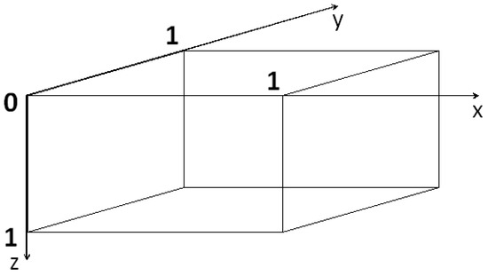
Figure 1.
Domain . Variable z means the depth; variables x and y are horizontal ones.
Let . We can write Equation (36) as
In the same way, higher-order approximations with more accuracy for the boundary and interior nodes are also obtained.
The purpose of this paper is to develop numerical methods and investigate regularization techniques to solve certain ill-posed problems for the 3D acoustic wave equation.
3.1. Reducing to Cube Domains
We first discretize BVP (1)–(5), (7) in all three dimensions on a uniform grid with grid points , for which we consider a cube domain where . If , then we can separate our region into subintervals and along the x, y, and z axes with the current time frame t. The goal is to approximate all the solutions, , where , and
As we have seen from Equation (37), any point in the region is related to the six points surrounding it. Consider a sketch of a region where , and . Here, the cross sections of our cube can be viewed at different z values. Note that many of the values in this region are already defined. From the boundary conditions, it is known that , and . The remaining points will be approximated by building a linear system of equations. We will create a system of equations , one for each solution at an internal point of our cube by iterating through all possible values of i, j, and k, where , and .
Corollary 2.
Corollary 3.
For example, if we work with the , and subintervals, the system of linear equations can be written in corresponding matrices and vectors as
where is the vector of approximate solutions at each point in the domain, A is the coefficient matrix of these solutions, is the boundary and initial condition vector at these points, and is the vector of the source function. Although Equation (38) is the same as for the two-dimensional case, the coefficient matrix A and the boundary and initial condition vector will have some different patterns.
3.2. Time Adaptivity
Time increments are used by time-adaptivity algorithms depending upon the medium in which they are adjusted, and by employing intermediate time steps, stability limits can be satisfied on each subregion of the domain. Depending on the algorithm used, these intermediate intervals of time can be chosen. According to [81], with the lowest propagation velocity, the discretization value ensures stability for the subregion.
3.3. Direct or Iterative Solution
For a system of small unknowns , the direct Gaussian elimination method can be used to solve the above system of equations. Iterative methods achieve a better result for large linear systems. According to [82], the accuracy of the numerical results greatly depends on the computational grid for all numerical methods based on the grid. For accuracy, a grid-converged solution would be preferred (i.e., the solution does not change significantly when more grid points are used as one approaches a tolerance point). For this work, three different iterative techniques are proposed to be used. Details of each iterative technique are provided in the following.
If we apply Equation (28) or (29) to solve the system of finite difference equations for the 3D acoustic wave equation, we obtain the Jacobi iteration formula (see [32]), as follows
The superscript n is an iterative index. To produce , we set the initial iterative guess at , and based on the iteration, it improves successively. From Equation (39), we find the next iteration for each point in the grid across all points in the grid in the horizontal rows. In the interior grid for all points when the iteration is completed, the difference between the vectors of the next iteration and the previous iteration is calculated. We set the predefined condition (tolerance) for the iteration to converge, and once the tolerance is met, the iteration ends and the solution to (39) is ; otherwise, the iterations continue, i.e.,
If we apply Equation (31) or (32) to solve the system of finite difference equations for the 3D acoustic wave equation, we obtain the Gauss–Seidel iteration formula (see [82]), as follows:
as can be seen in Equation (40), the values and are already updated as one moves through the grids to reach the grid point . The implementation of this iteration method follows the Jacobi method.
The most widely used iteration method is the SOR method and is integrated into the Gauss–Seidel method. With the aim of speedy convergence, a relaxation parameter is included in the Gauss–Seidel iteration method. Using (33) or (34), we obtain the SOR iteration formula (see [83]), as follows:
the relaxation parameter is in the range . The implementation of the SOR method follows the first two iteration methods.
To solve Equation (9) using an iterative method, performing a matrix vector product is the main cost. However, in practice, making this a matrix-free method, the matrix A is never generated or stored. To produce the action of A on q, a MATLAB code can be created using the finite difference algorithm.
MATLAB programs are developed for all three iterative techniques using the finite difference method with Dirichlet and Neumann boundary conditions that are applied at the boundary of the domain. The results of our discretization and iterative approximations for the sample problem can be examined with a larger mesh size in different time frames. Our Jacobi, Gauss–Seidel, and SOR iterations will use an RMS residual tolerance of , for the values of , and in different time frames, the time interval used for the Jacobi, Gauss–Seidel, and SOR iterative methods for stability. For the values of and in different time frames, the time interval used for the SOR iterative method for stability in test problem 1.
We compare the exact solution with the continuous problem with the solution of the discretized problem computed using iteration techniques.
4. Numerical Experiments
4.1. Test Problem 1: A Known Analytical Solution
4.2. Results
From Table 2, we can check the numerical performance of iterative methods, Jacobi, Gauss–Seidel, and SOR (with relaxation parameter ) in three dimensions to solve the acoustic wave equation for the values of , and in different time frames t.

Table 2.
Numerical results obtained for test problem 1 using Jacobi, Gauss–Seidel, and SOR iterative methods.
In Table 2, the first column represents the mesh size, the second column shows the current time t, the third column represents the error of the numerical method, the fourth column shows the error of the inverse problem, and the fifth column shows the number of iterations taken by the Jacobi, Gauss–Seidel, and SOR iterative methods for the chosen tolerance of until convergence in the relative residual. The last column shows the wall clock time for each and every run.
From Table 3, we can check the , , and norms of the Jacobi, Gauss–Seidel, and SOR methods in three dimensions to solve the acoustic wave equation for the values of , and in different time frames. Here, the norm is the spectral radius of the matrix A.

Table 3.
, , and norms obtained for test problem 1 using Jacobi, Gauss–Seidel, and SOR iterative methods.
From Table 4, we can check the numerical performance of the 3D—SOR method in three dimensions to solve the acoustic wave equation for the values of , , and with several relaxation parameters in time and for the values of , , and with relaxation parameters in different time frames t.

Table 4.
Numerical results obtained for test problem 1 using SOR iterative method.
In Table 4, the first column represents the mesh size, the second column is the relaxation parameter, the third column shows the current time t, the fourth column represents the error of the numerical method, the fifth column shows the error of the inverse problem, and the sixth column shows the number of iterations taken by the SOR iterative method for the chosen tolerance of until convergence in the relative residual. The last column shows the wall clock time for each and every run.
From Table 5, we can check the , , and norms of the SOR method in three dimensions to solve the acoustic wave equation for the values of , , and in different time frames. Here, the norm is the spectral radius of the matrix A.

Table 5.
, , and norms obtained for test problem 1 using SOR iterative method.
4.3. Comparison of Iterative Methods
As mentioned above, we have shown that sophisticated iterative methods have converged in fewer iterations within a shorter run time of the wall clock. Now, our aim is to characterize the differences in convergence rate further in terms of iterations. To do that, we have taken the spectral radius of the iteration matrix, from each method with the same grid size of in different time frames t. Then we plot the relative residuals versus the iteration number and compare the results of each method, shown in Figure 2 and Figure 3 of this result with two visualizations. Figure 2a and Figure 3a depict the convergence of each iterative method with the grid size at time , , and Figure 2b and Figure 3b show the same data, but only for the first 1000 iterations to take a closer look at the iterative methods, which converge much faster.
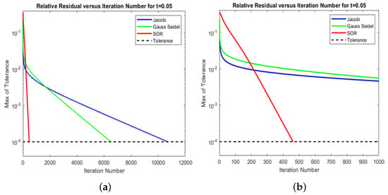
Figure 2.
Comparison of three different iterative methods in test problem 1: (a) The relative residual versus the iteration number for each iterative method with grid at the time on a semilog plot (b); the same data as (a), but only the first 1000 iterations.
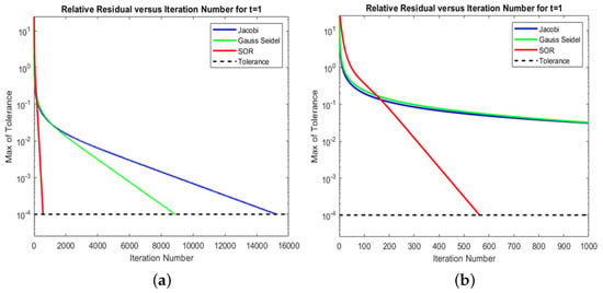
Figure 3.
Comparison of three different iterative methods in test problem 1: (a) The relative residual versus the iteration number for each iterative method with grid at the time on a semilog plot (b); the same data as (a), but only the first 1000 iterations.
4.4. Comparison of Analytical and Numerical Solutions
From Figure 4, Figure 5, Figure 6, Figure 7 and Figure 8, we can see the sound pressure distribution from low and high levels in a three-dimensional cube for the analytical and numerical solutions of test problem 1.
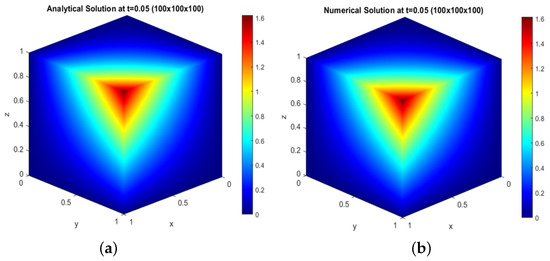
Figure 4.
For the grid : (a) analytical solution at ; (b) numerical solution at
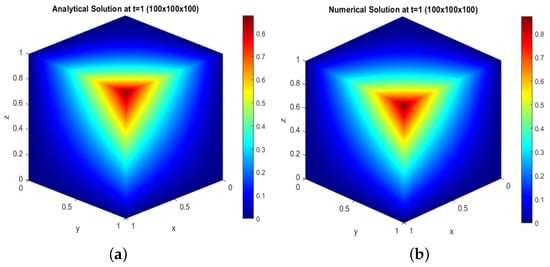
Figure 5.
For the grid : (a) analytical solution at ; (b) numerical solution at
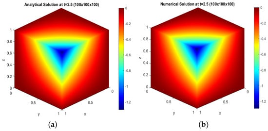
Figure 6.
For the grid : (a) analytical solution at ; (b) numerical solution at
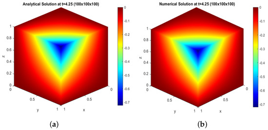
Figure 7.
For the grid : (a) analytical solution at ; (b) numerical solution at
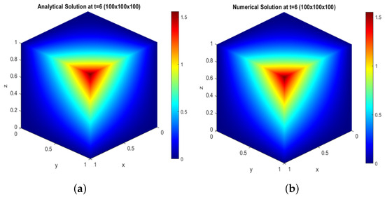
Figure 8.
For the grid : (a) analytical solution at ; (b) numerical solution at
We plot and compare the analytical and numerical solutions shown in Figure 4, Figure 5, Figure 6, Figure 7 and Figure 8 with two visualizations of the result. Figure 4a, Figure 5a, Figure 6a, Figure 7a, and Figure 8a show the sound pressure distribution from low to high level, from high to low level in a cube for the size of the grid at time , and Figure 4b, Figure 5b, Figure 6b, Figure 7b, and Figure 8b shows the same result, but for the numerical solution.
4.5. Error Graphs
We plot the error difference between the analytical and numerical solutions, shown in Figure 9 and Figure 10. Figure 9a,b and Figure 10a,b depict the error difference between the analytical and numerical solutions at time for the size of the grid .
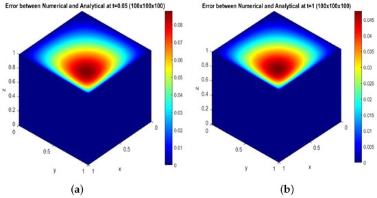
Figure 9.
Error between analytical and numerical solution(): (a) at ; (b) at
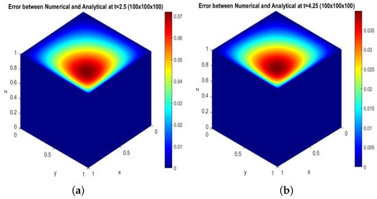
Figure 10.
Error between analytical and numerical solution(): (a) at ; (b) at
From Table 6, we can check the maximum error between the analytical and numerical solution using the Jacobi, Gauss–Seidel, and SOR methods in three dimensions to solve the acoustic wave equation for the values of , , and in different time frames t.

Table 6.
Maximum error between analytical and numerical solution obtained for test problem 1 using the Jacobi Gauss–Seidel and SOR iterative methods.
The results of our discretization and iterative approximations with a larger grid size in different time frames for test problem 2 can be examined. Our SOR iterations will use an RMS residual tolerance of , for the values of and in different time frames, the time interval used for the SOR iterative method for stability.
We compare the exact solution with the continuous problem with the solution of the discretized problem computed using the SOR iteration technique.
4.6. Test Problem 2: A Known Analytical Solution
4.7. Results
From Table 7, we can check the numerical performance of the 3D—SOR method in three dimensions to solve the acoustic wave equation for the values of , , and in different time frames t.

Table 7.
Numerical results obtained for test problem 2 using SOR iterative method.
The top panel of Table 7 shows the results of the 3D-SOR iterative method for test problem 2. The first column represents the size of the mesh, the second column shows the relaxation parameter, the third column shows the current time t, the fourth column represents the error of the numerical method, the fifth column shows the error of the inverse problem, and the sixth column shows the number of iterations taken by the SOR iterative method for the chosen tolerance of until convergence in the relative residual. The last column shows the wall clock time for each and every run.
From Table 8, we can check the , , and norms of the SOR method in three dimensions to solve the acoustic wave equation for the values of , , and in different time frames. Here, the norm is the spectral radius of the matrix A.

Table 8.
, , and norms obtained for test problem 2 using SOR iterative method.
4.8. Comparison of Analytical and Numerical Solutions
From Figure 11, Figure 12 and Figure 13, we can see the sound pressure distribution from low and high levels in a three-dimensional cube for the analytical and numerical solutions of test problem 2.

Figure 11.
For the grid : (a) analytical solution at ; (b) numerical solution at
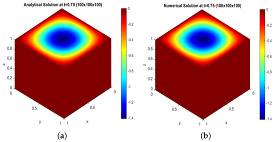
Figure 12.
For the grid : (a) analytical solution at ; (b) numerical solution at
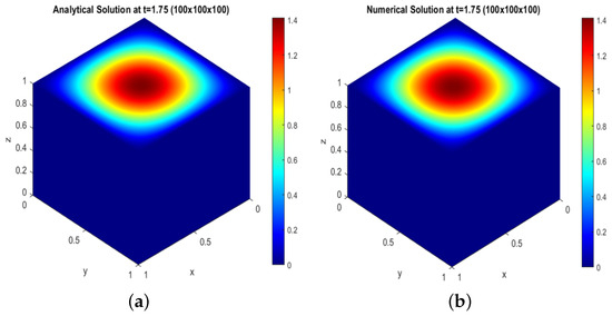
Figure 13.
For the grid : (a) analytical solution at ; (b) numerical solution at
We plot and compare the analytical and numerical solutions shown in Figure 11, Figure 12 and Figure 13 with two visualizations of the result. Figure 11a, Figure 12a, and Figure 13a show the sound pressure distribution from low to high level and from high to low level in a cube for the size of the grid at time , and Figure 11b, Figure 12b, and Figure 13b show the same result, but for the numerical solution.
4.9. Error Graphs
We plot the error difference between the analytical and numerical solutions, shown in Figure 14 with two visualizations of this result. Figure 14a depicts the error difference between the analytical and numerical solutions at time for the size of the grid , and Figure 14b shows the same result, but at time .
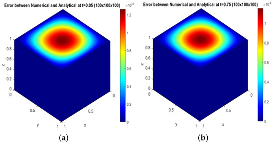
Figure 14.
Error between analytical and numerical solution(): (a) at ; (b) at
From Table 9, we can check the maximum error between the analytical and numerical solution using the SOR method in three dimensions to solve the acoustic wave equation for the values of , , and in different time frames t.

Table 9.
Maximum error between analytical and numerical solution obtained for test problem 2 using the SOR iterative method.
5. Discussion
In this paper, using an explicit finite difference method in the time domain, we find the numerical solution of the 3D-acoustic wave equation in a cube through three different iterative techniques. We compared our numerical results with the known analytical solution through numerical experiments, checked the results for stability with larger grid size, and also found the better iterative technique among three.
From Table 2 and Table 3, we compare the numerical performances of Jacobi, Gauss–Seidel, and SOR iterative methods in three dimensions to solve the acoustic wave equation in different time periods for test problem 1. We observe that all three iterative methods are accurate; however, the Jacobi iterative method is much slower than the other two iterative methods and does not converge in a reasonable amount of time for the higher values of , , and ; we checked the numerical results of the Gauss–Seidel iterative method for the same values of , , and . Compared with the Jacobi iterative method, the Gauss–Seidel iterative method requires about more than half of the iterations and fewer execution times than the Jacobi iterative method. However, the number of iterations required for this method is unacceptable for a larger grid size.
The SOR iterative method can solve large linear systems in a faster way than Jacobi, and the Gauss–Seidel methods and convergence for the higher values of , , and are significantly faster than the other two iterative methods. We saw that the SOR method has a much lower iteration count and shorter runtime with relaxation parameter than the Jacobi and Gauss–Seidel methods. Specifically, for , , and , at time , the Gauss–Seidel method took 10891 iterations and the execution time is 405.187567 s versus the SOR method, which took only 647 iterations and only 24.908182 s with the relaxation parameter . We checked the SOR method at several values of the relaxation parameter at time (see Table 4) and observed that, at (see Table 2), this method requires fewer iterations and fewer execution times.
From Table 6, we checked the difference in error between the analytical and numerical solutions at different time periods for the Jacobi, Gauss–Seidel, and SOR iterative schemes for test problem 1. We saw slightly less error difference at time compared with the other time periods that we checked in the problem between the analytical and numerical solutions for the three iterative schemes.
From Table 7 and Table 8, we checked the numerical performance of the SOR iterative method in three dimensions in solving the acoustic wave equation in different time periods for test problem 2. From Table 9, we checked the difference in error between the analytical and numerical solutions at different time periods for the SOR iterative scheme for test problem 2. We saw slightly less error difference at time compared with the other time periods that we checked in the problem between the analytical and numerical solutions for the SOR iterative scheme.
In this work, we presented numerical results in the cubic domain and also checked numerical results for other geometric domains through MATLAB software and saw the efficiency of this method. Based on our numerical results, the finite difference method is relatively simple to implement for other geometric domains.
The finite difference method (FDM) has some limitations related to complex geometries, boundary conditions, and accuracy. Accuracy depends on grid spacing and time step, while complex shapes and non-straight boundaries are difficult to represent.
6. Conclusions
This research was considered to reconstruct the acoustic pressure in a cube through the numerical solution of the acoustic wave equation in the time domain. Under the finite difference method (FDM), three iterative schemes were compared, which are Jacobi, Gauss–Seidel, and SOR iterative schemes. The results achieved in this work clearly showed that the three iterative schemes are accurate and the SOR iterative scheme is more efficient in terms of fewer iterations, fewer execution times, and faster convergence compared with the other two iterative techniques.
Author Contributions
Methodology, G.B., S.C., S.K., and M.S.; software, S.C.; formal analysis, G.B., S.C., S.K., and M.S.; writing—original draft preparation, S.C.; writing—review and editing, G.B., S.C., S.K., and M.S.; supervision, S.K. All authors have read and agreed to the published version of the manuscript.
Funding
Research by authors G.B., S.K., and M.S. has been funded by the Science Committee of the Ministry of Science and Higher Education of the Republic of Kazakhstan (Grant No. AP 19678469). The work of author S.C. is supported by the Mathematical Centre in Akademgorodok under the Agreement No. 075-15-2022-281 with the Ministry of Science and Higher Education of the Russian Federation.
Data Availability Statement
The original contributions presented in this study are included in the article. Further inquiries can be directed to the corresponding author(s).
Conflicts of Interest
The authors declare no conflicts of interest.
Abbreviations
| FDM | finite difference method |
| PDEs | partial differential equations |
| SLAE | system of linear algebraic equations |
| SOR | successive over-relaxation |
References
- John, F. Continuous dependence on data for solutions of partial differential equations with a prescribed bound. Pure Appl. Math. 1960, 4, 551–585. [Google Scholar] [CrossRef]
- John, F. Differential Equations with Approximate and Improper Data; Lectures. N. Y.; New York University: New York, NY, USA, 1995. [Google Scholar]
- Douglas, J. A Numerical Method for Analytic Continuation, Boundary Value Problems in Differential Equations; University of Wisconsin Press: Madison, WI, USA, 1960; pp. 179–189. [Google Scholar]
- Cannon, J.R. Error estimates for some unstable continuation problems. J. Soc. Ind. Appl. Math. 1964, 12, 270–284. [Google Scholar] [CrossRef]
- Cannon, J.R.; Miller, K. Some problems in numerical analytic continuation. J. SIAM Numer. Anal. 1965, 2, 87–98. [Google Scholar] [CrossRef]
- Lavrentiev, M.M.; Romanov, V.G.; Shishat ski, S.P. Ill-Posed Problems of Mathematical Physics and Analysis; American Mathematical Soc.: Providence, RI, USA, 1986. [Google Scholar]
- Hadamard, J. Lectures on Cauchy’s Problem in Linear Partial Differential Equations; Yale Univ. Press: New Haven, CT, USA, 1923. [Google Scholar]
- Payne, L.E. Improperly Posed Problems in Partial Differential Equation; SIAM: Philadelphia, PA, USA, 1975. [Google Scholar]
- Finch, D.; Patch, S.K. Determining a function from its mean values over a family of spheres. SIAM J. Math. Anal. 2004, 35, 1213–1240. [Google Scholar] [CrossRef]
- Natterer, F. Photo-acoustic inversion in convex domains. Inverse Probl. Imaging. 2012, 6, 1–6. [Google Scholar] [CrossRef]
- Symes, W.W. A trace theorem for solutions of the wave equation, and the remote determination of acoustic sources. Math. Meth. Appl. Sci. 1983, 5, 131–152. [Google Scholar] [CrossRef]
- Romanov, V.G. An asymptotic expansion for a solution to viscoelasticity equations. Eurasian J. Math. Comput. Appl. 2013, 1, 42–62. [Google Scholar] [CrossRef]
- Romanov, V.G. Estimation of the solution stability of the Cauchy problem with the data on a time-like plane. J. Appl. Industr. Math. 2018, 12, 531–539. [Google Scholar] [CrossRef]
- Romanov, V.G. Regularization of a solution to the Cauchy problem with data on a timelike plane. Sib. Math. J. 2018, 59, 694–704. [Google Scholar] [CrossRef]
- Romanov, V.G.; Bugueva, T.V.; Dedok, V.A. Regularization of the solution of the Cauchy problem: The quasi-reversibility method. J. Appl. Industr. Math. 2018, 12, 716–728. [Google Scholar] [CrossRef]
- Kabanikhin, S.I.; Shishlenin, M.A. Theory and numerical methods for solving inverse and ill-posed problems. J. Inverse Ill-Posed Probl. 2019, 27, 453–456. [Google Scholar] [CrossRef]
- Kabanikhin, S.I.; Scherzer, O.; Shishlenin, M.A. Iteration methods for solving a two-dimensional inverse problem for a hyperbolic equation. J. Inverse-Ill-Posed Probl. 2003, 11, 87–109. [Google Scholar] [CrossRef]
- Kabanikhin, S.I. Inverse and Ill-Posed Problems; De Gruyter: Berlin, Germany, 2012. [Google Scholar]
- Lavrent’ev, M.M.; Savel’ev, L.J. Operator Theory and Ill-Posed Problems; Walter de Gruyter: Berlin, Germany, 2006. [Google Scholar]
- Lions, J.L.; Magenes, E. Non-Homogeneous Boundary Value Problems and Applications; Springer: Berlin/Heidelberg, Germany, 1972. [Google Scholar]
- Romanov, V.G.; Kabanikhin, S.I. Inverse Problems of Geoelectrics; VNU Science: Utrecht, The Netherlands, 1994. [Google Scholar]
- Weston, V.H. Invariant imbedding and wave splitting in R3, Part II. The Green function approach to inverse scattering. Inverse Probl. 1992, 8, 919–947. [Google Scholar] [CrossRef]
- Weston, V.H.; He, S. Wave-splitting of the telegraph equation in R3 and its application to the inverse scattering. Inverse Probl. 1993, 9, 789–813. [Google Scholar] [CrossRef]
- Romanov, V.G. On a Numerical Method for Solving a Certain Inverse Problem for a Hyperbolic Equation. Sib. Math. J. 1996, 37, 633–655. [Google Scholar] [CrossRef]
- Romanov, V.G. A Local Version of the Numerical Method for Solving an Inverse Problem. Sib. Math. J. 1996, 37, 904–918. [Google Scholar] [CrossRef]
- Helsing, J.; Johansson, B. Fast reconstruction of harmonic functions from cauchy data using the dirichlet-to-neumann map and integral equations. Inverse Probl. Sci. Eng. 2011, 19, 717–727. [Google Scholar] [CrossRef]
- Kabanikhin, S.I.; Nurseitov, D.; Shishlenin, M.A.; Sholpanbaev, B.B. Inverse Problems for the Ground Penetrating Radar. J. Inverse-Ill-Posed Probl. 2013, 21, 885–892. [Google Scholar] [CrossRef]
- Kabanikhin, S.I.; Gasimov, Y.S.; Nurseitov, D.B.; Shishlenin, M.A.; Sholpanbaev, B.B.; Kasenov, S. Regularization of the continuation problem for elliptic equations. J. Inverse-Ill-Posed Probl. 2013, 21, 871–884. [Google Scholar] [CrossRef]
- Kabanikhin, S.I.; Shishlenin, M.A. Regularization of the decision prolongation problem for parabolic and elliptic elliptic equations from border part. Eurasian J. Math. Comput. Appl. 2014, 2, 81–91. [Google Scholar]
- Kabanikhin, S.I.; Shishlenin, M.A.; Nurseitov, D.B.; Nurseitova, A.T.; Kasenov, S.E. Comparative analysis of methods for regularizing an initial boundary value problem for the Helmholtz equation. J. Appl. Math. 2014, 2014, 786326. [Google Scholar] [CrossRef]
- Keran, L.; Wenyuan, L. An efficient and high accuracy finite-difference scheme for the acoustic wave equation in 3D heterogeneous media. J. Comput. Sci. 2020, 40, 101063. [Google Scholar] [CrossRef]
- Causon, D.M.; Mingham, C.G. Introductory Finite Difference Methods for PDES; Ventus Publishing ApS: London, UK, 2010; p. 144. [Google Scholar]
- Alford, R.; Kelly, K.; Boore, D.M. Accuracy of finite-difference modeling of the acoustic wave equation. Geophysics 1974, 39, 834–842. [Google Scholar] [CrossRef]
- Tam, C.K.; Webb, J.C. Dispersion-relation-preserving finite difference schemes for computational acoustics. J. Comput. Phys. 1993, 107, 262–281. [Google Scholar] [CrossRef]
- Yang, D.; Tong, P.; Deng, X. A central difference method with low numerical dispersion for solving the scalar wave equation. Geophys. Prospect 2012, 60, 885–905. [Google Scholar] [CrossRef]
- Liao, H.L.; Sun, Z.Z. Maximum norm error estimates of efficient difference schemes for second-order wave equations. J. Comput. Appl. Math. 2011, 235, 2217–2233. [Google Scholar] [CrossRef]
- Finkelstein, B.; Kastner, R. Finite difference time domain dispersion reduction schemes. J. Comput. Phys. 2017, 221, 422–438. [Google Scholar] [CrossRef]
- Zapata, M.; Balam, R.; Urquizo, J. High-order implicit staggered grid finite differences methods for the acoustic wave equation. Numer. Methods Partial Differ. Equ. 2018, 34, 602–625. [Google Scholar] [CrossRef]
- Alexandre, J.M.A.; Regina, C.P.L.; Otton, T.S.F.; Elson, M.T. Finite difference method for solving acoustic wave equation using locally adjustable time-steps. Procedia Comput. Sci. 2014, 29, 627–636. [Google Scholar] [CrossRef][Green Version]
- Liu, Y.; Sen, M.K. An implicit staggered-grid finite-difference method for seismic modelling. Geophys. J. Int. 2009, 179, 459–474. [Google Scholar] [CrossRef]
- Liu, Y.; Mrinal, K. A new time-space domain high-order finite-difference method for the acoustic wave equation. J. Comput. Phys. 2009, 228, 8779–8806. [Google Scholar] [CrossRef]
- Liu, Y.; Sen, M. Acoustic VTI modeling with a time-space domain dispersion-relation-based finite-difference scheme. Geophysics 2010, 75, 11–17. [Google Scholar] [CrossRef]
- Liang, W.; Yang, C.; Wang, Y.; Liu, H. Acoustic wave equation modeling with new time-space domain finite difference operators. Chin. J. Geophys. 2013, 56, 3497–3506. [Google Scholar]
- Liao, W.; Yong, P.; Dastour, H.; Huang, J. Efficient and accurate numerical simulation of acoustic wave propagation in a 2d heterogeneous media. Appl. Math. Comput. 2018, 321, 385–400. [Google Scholar] [CrossRef]
- Young, D.M. Iterative Solution of Large Linear Systems; Academic Press: New York, NY, USA, 1971. [Google Scholar]
- Dancis, J. The optimal ω is not best for the SOR iteration method. Linear Algebra Its Appl. 1991, 154–156, 819–845. [Google Scholar] [CrossRef]
- Rigal, A. Convergence and optimization of successive overrelaxation for linear systems of equations with complex eigenvalues. J. Comput. Phys. 1979, 32, 10–23. [Google Scholar] [CrossRef]
- Hadjidimos, A. Successive overrelaxation (SOR) and related methods. J. Comput. Appl. Math. 2000, 123, 177–199. [Google Scholar] [CrossRef]
- Britt, S.; Turkel, E.; Tsynkov, S. A high order compact time/space finite difference scheme for the wave equation with variable speed of sound. J. Sci. Comput. 2018, 76, 777–811. [Google Scholar] [CrossRef]
- Mohammadi, V.; Dehghan, M.; Mesgarani, H. The localized RBF interpolation with its modifications for solving the incompressible two-phase fluid flows: A conservative Allen–Cahn–Navier–Stokes system. Eng. Anal. Bound. Elem. 2024, 168, 105908. [Google Scholar] [CrossRef]
- Qu, W.; Gu, Y.; Zhang, Y.; Fan, C.M.; Zhang, C. A combined scheme of generalized finite difference method and Krylov deferred correction technique for highly accurate solution of transient heat conduction problems. Int. J. Numer. Methods Eng. 2018, 117, 63–83. [Google Scholar] [CrossRef]
- Qu, W.; Fan, C.M.; Zhang, Y. Analysis of three-dimensional heat conduction in functionally graded materials by using a hybrid numerical method. Int. J. Heat Mass Transf. 2019, 145, 118771. [Google Scholar] [CrossRef]
- Belonosov, A.; Shishlenin, M.; Klyuchinskiy, D. A comparative analysis of numerical methods of solving the continuation problem for 1D parabolic equation with the data given on the part of the boundary. Adv. Comput. Math. 2019, 45, 735–755. [Google Scholar] [CrossRef]
- Chung, E.; Ito, K.; Yamamoto, M. Least squares formulation for ill-posed inverse problems and applications. Appl. Anal. 2021, 101, 5247–5261. [Google Scholar] [CrossRef]
- Desiderio, L.; Falletta, S.; Ferrari, M.; Scuderi, L. CVEM-BEM Coupling for the Simulation of Time-Domain Wave Fields Scattered by Obstacles with Complex Geometries. Comput. Methods Appl. Math. 2023, 23, 353–372. [Google Scholar] [CrossRef]
- Bzeih, M.; Arwadi, T.E.; Wehbe, A.; Madureira, R.L.R.; Rincon, M.A. A finite element scheme for a 2D-wave equation with dynamical boundary control. Math. Comput. Simul. 2023, 205, 315–339. [Google Scholar] [CrossRef]
- Duc, N.V.; Hao, D.N.; Shishlenin, M. Regularization of backward parabolic equations in Banach spaces by generalized Sobolev equations. J. Inverse Ill Posed Probl. 2024, 32, 9–20. [Google Scholar] [CrossRef]
- Burman, E.; Delay, G.; Ern, A. The unique continuation problem for the Heat equation discretized with a high-order space-time nonconforming method. SIAM J. Numer. Anal. 2023, 61, 2534–2557. [Google Scholar] [CrossRef]
- Dahmen, W.; Monsuur, H.; Stevenson, R. Least squares solvers for ill-posed PDEs that are conditionally stable. ESAIM Math. Model. Numer. Anal. 2023, 57, 2227–2255. [Google Scholar] [CrossRef]
- Helin, T. Least Squares approximations in linear statistical inverse learning problems. SIAM J. Numer. Anal. 2024, 62, 2025–2047. [Google Scholar] [CrossRef]
- Epperly, E.N. Fast and Forward stable randomized algorithms for linear least-squares problems. SIAM J. Matrix Anal. Appl. 2024, 45, 1782–1804. [Google Scholar] [CrossRef]
- Qu, W.; Gu, Y.; Fan, C.M. A stable numerical framework for long-time dynamic crack analysis. Int. J. Solids Struct. 2024, 293, 112768. [Google Scholar] [CrossRef]
- Li, H. Projected Newton method for large-scale bayesian linear inverse problems. SIAM J. Optim. 2025, 35, 1439–1468. [Google Scholar] [CrossRef]
- Bakanov, G.; Chandragiri, S.; Shishlenin, M.A. Jacobi numerical method for solving 3D continuation problem for wave equation. Sib. Electron. Math. Rep. 2025, 22, 428–442. [Google Scholar]
- Kabanikhin, S.I. Definitions and examples of inverse and ill-posed problems. J. Inverse Ill-Posed Probl. 2008, 16, 317–357. [Google Scholar] [CrossRef]
- Marin, L.; Elliott, L.; Heggs, P.J.; Ingham, D.B.; Lesnic, D.; Wen, X. Conjugate gradient-boundary element solution to the Cauchy problem for Helmholtz-type equations. Comput. Mech. 2003, 31, 367–377. [Google Scholar] [CrossRef]
- Marin, L.; Elliott, L.; Heggs, P.J.; Ingham, D.B.; Lesnic, D.; Wen, X. Comparison of regularization methods for solving the Cauchy problem associated with the Helmholtz equation. Int. J. Numer. Methods Eng. 2004, 60, 1933–1947. [Google Scholar] [CrossRef]
- Qin, H.; Wei, T.; Shi, R. Modified Tikhonov regularization method for the Cauchy problem of the Helmholtz equation. J. Comput. Appl. Math. 2009, 224, 39–53. [Google Scholar] [CrossRef]
- Reginska, T.; Reginski, K. Approximate solution of a Cauchy problem for the Helmholtz equation. Inverse Probl. 2006, 22, 975–989. [Google Scholar] [CrossRef]
- Reginiska, T.; Tautenhahn, U. Conditional stability estimates and regularization with applications to Cauchy problems for the Helmholtz equation. Numer. Funct. Anal. Optim. 2009, 30, 1065–1097. [Google Scholar] [CrossRef]
- Isakov, V.; Kindermann, S. Subspaces of stability in the Cauchy problem for the Helmholtz equation. Methods Appl. Anal. 2011, 18, 1–30. [Google Scholar] [CrossRef]
- Axelsson, O. Iterative Solution Methods; Cambridge University Press: Cambridge, UK, 1994. [Google Scholar]
- Strikwerda, J.C. Finite Difference Schemes and Partial Differential Equations, 2nd ed.; SIAM: Philadelphia, PA, USA, 2004. [Google Scholar]
- Saad, Y. Iterative Methods for Sparse Linear Systems; Society for Industrial and Applied Mathematics: Philadelphia, PA, USA, 2003. [Google Scholar]
- Smith, G.D. Numerical Solution of Partial Differential Equations Finite Difference Methods, 3rd ed.; Oxford University Press: New York, NY, USA, 1985. [Google Scholar]
- Burden, R.L.; Douglas, J.F. Numerical Analysis; Cengage Learning: Toronto, ON, Canada, 2010. [Google Scholar]
- Ames, W.F. Numerical Methods for Partial Differential Equations, 2nd ed.; Academic Press: New York, NY, USA, 1977. [Google Scholar]
- Demmel, J.W. Applied Numerical Linear Algebra; SIAM: Philadelphia, PA, USA, 1997. [Google Scholar]
- Press, W.H.; Teukolsky, S.A.; Vetterling, W.T.; Flannery, B.P. Numerical Recipes Third Edition; Cambridge University Press: New York, NY, USA, 2007. [Google Scholar]
- Nagel, J.R. Numerical solutions to Poisson equations using the Finite difference method. IEEE Antennas Propag. Mag. 2014, 56, 209–224. [Google Scholar] [CrossRef]
- Falk, J.; Tessmer, E.; Gajewski, D. Efficient finite-difference modelling of seismic waves using locally adjustable time steps. Geophys. Prospect. 1998, 46, 603–616. [Google Scholar] [CrossRef]
- Vendromin, C.J. Numerical Solutions of Laplace’s Equation for Various Physical Situations; Brock University: St. Catharines, ON, Canada, 2017. [Google Scholar]
- Yang, X.I.A.; Mittal, R. Acceleration of the Jacobi Iterative Method by factors exceeding 100 using Scheduled Relaxation. J. Comput. Phys. 2014, 274, 695–708. [Google Scholar] [CrossRef]
Disclaimer/Publisher’s Note: The statements, opinions and data contained in all publications are solely those of the individual author(s) and contributor(s) and not of MDPI and/or the editor(s). MDPI and/or the editor(s) disclaim responsibility for any injury to people or property resulting from any ideas, methods, instructions or products referred to in the content. |
© 2025 by the authors. Licensee MDPI, Basel, Switzerland. This article is an open access article distributed under the terms and conditions of the Creative Commons Attribution (CC BY) license (https://creativecommons.org/licenses/by/4.0/).