Optimization of EHA Hydraulic Cylinder Buffer Design Using Enhanced SBO–BP Neural Network and NSGA-II

Abstract

In order to solve a certain type of Electro-Hydrostatic Actuators (EHA) hydraulic cylinder small cavity buffer end impact problem, based on AMESim to establish a hydraulic cylinder small cavity buffer machine–hydraulic joint simulation model. First, four important structural parameters, namely, the fitting clearance G of the buffer sleeve and buffer hole, the fixed orifice D, the wedge face angle $\theta$, and the wedge face length L₁ were selected to analyze their influence on the pressure of the buffer chamber and the end speed of the piston. Second, enhanced Social Behavior Optimization (SBO) was used to optimize the back-propagation neural network (BP) model to construct a prediction model for the buffer time T of the small chamber of the hydraulic cylinder, the end-piston speed V_e, the rate of change of the end-piston speed V_r, and the return speed of the hydraulic oil V_h. The SBO–BP model performed well in several key performance evaluation metrics, showing better prediction accuracy and generalization performance. Finally, the multi-objective Non-dominated Sorting Genetic Algorithm II (NSGA-II) was used to optimize the hydraulic cylinder small-cavity buffer structure using the multi-objective NSGA-II with the objectives of the shortest buffer time, the minimum end-piston speed, the minimum change rate of the end-piston speed, and the minimum hydraulic oil reflux speed. The optimized design reduced the piston end speed from 0.060 m/s to 0.032 m/s, corresponding to a 46.7% improvement. The findings demonstrate that the proposed hybrid optimization approach effectively alleviates the end-impact problem of EHA small-cavity buffers and provides a novel methodology for achieving high-performance and reliable actuator designs.

1. Introduction

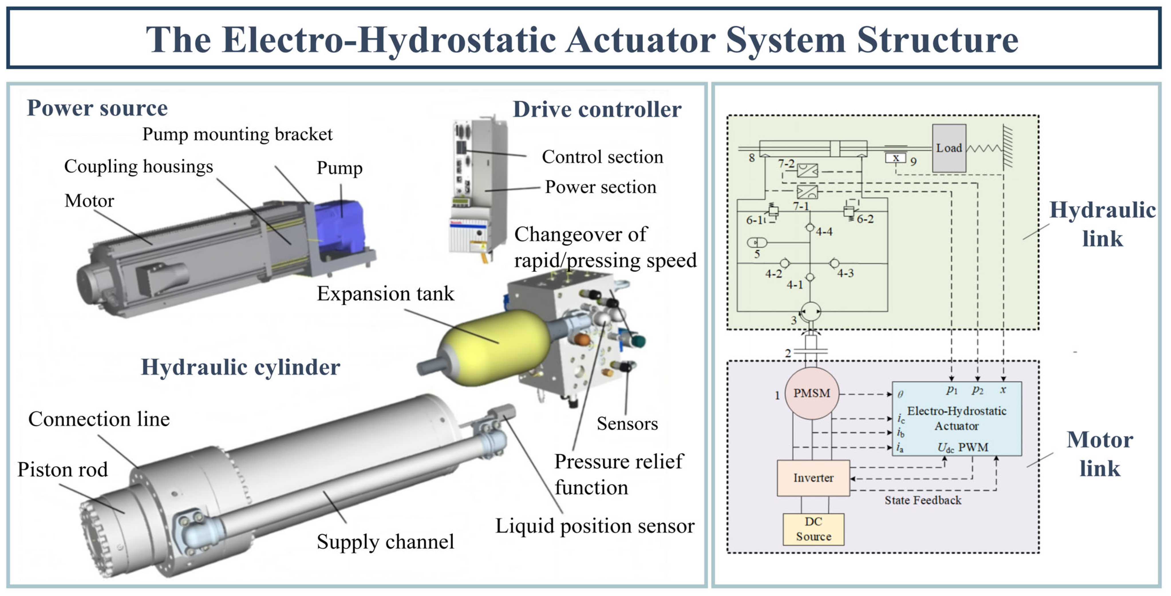
An electro-hydrostatic actuator is a highly integrated closed pump-controlled electro-hydraulic servo system, which is mainly composed of three parts: power source, drive controller, and hydraulic actuator, and its core components include a permanent magnet synchronous motor (PMSM), piston pump and hydraulic cylinder, etc., as shown in Figure 1. An EHA controls the flow output of the piston pump by adjusting the rotational speed and direction of the motor, thus driving the piston of the hydraulic cylinder to produce reciprocating expansion and contraction movements to achieve linear displacement output. The system combines the advantages of electric drive and hydraulic transmission, featuring fast response speed, high output force and compact structure. Compared with the traditional motor actuator, an EHA effectively avoids the stall problem caused by the mechanical structure [1] and does not need to configure servo valves, tanks and other external hydraulic components, so it has high integration, high power density, high reliability and good maintainability [2]. At present, EHA technology has been widely used in aerospace, marine valves, robotics and other high-end equipment manufacturing fields [3,4,5].

However, as a higher-order nonlinear system consisting of mechanical, electrical and hydraulic couplings, the EHA suffers from hydraulic cylinder end impacts during operation [6]. The problem mainly manifests in the hydraulic cylinder piston near the end of the stroke, due to drastic changes in the buffer chamber pressure and the speed at the end of the piston stroke rising too high. This can easily lead to mechanical impacts as the piston moves inside the cylinder body, thus triggering shock vibration, which affects the stability of the system and its useful life. The research shows that the end impact characteristics are significantly affected by a number of buffer structure parameters, including the fitting clearance between the buffer sleeve and buffer holes, the diameter of the fixed throttle holes, the angle and length of the wedge surface, etc., the combination of which undoubtedly increases the complexity of the design of high-precision, high-performance controllers.

As an indispensable actuating element in the hydraulic system, the hydraulic cylinder usually needs to be set up with an effective buffer structure to inhibit the end impact due to its long working hours, large load carrying capacity and fast movement speed. In practice, most of the hydraulic cylinder cushioning structures are incomplete cushioning, i.e., there is still a certain terminal speed of the piston at the end of the stroke. When this speed exceeds the safety limit allowed by the structure, it is very easy to produce impact problems [7,8,9]. Therefore, a reasonable buffer structure design must not only ensure that the buffer cavity peak pressure does not exceed the sealing system’s ability to withstand pressure, but also must control the speed of the piston to keep the impact strength within the allowable range.

Buffer structure is usually divided into two categories: external buffer structure and internal buffer structure. The external buffer structure is often formed with throttle valves, relief valves, accumulators, sequence valves, etc. to achieve the buffer function, while the internal buffer structure is directly embedded in the body of the hydraulic cylinder. In recent years, many scholars have made a lot of research in the design of buffer structure within the hydraulic cylinder. For example, Zhao X et al. designed a high-speed hydraulic cylinder buffer structure based on flat plate throttling and confirmed its effectiveness through simulation and testing [10]. Liu J et al. established a Simulink simulation model of a cylindrical buffer structure and constructed a multi-objective optimization function based on the end-piston speed and peak pressure to optimize the structural parameters [11]. Jiang H et al. derived the flow equations for a variety of internal buffer structures, such as cylindrical, step, conical, parabolic and row of holes, and analyzed their applicability scenarios [12]. Zhang T et al. used Fluent to numerically simulate a novel conical cushioning structure, revealing the effects of end clearance and external load on the cushioning performance [13]. Ma Z et al. proposed to design parallel dual oil chambers at the bottom of the hydraulic cylinder to achieve internal cushioning and analyzed the effects of spring stiffness, oil chamber diameter and oil viscosity on the cushioning effect through simulation [14]. Zhu T et al., on the other hand, proposed a cylindrical cushioning structure with a variable throttling area, and found that the unilateral clearance had the most significant effect on the cushioning performance [15].

With the rapid development of artificial intelligence technology, machine learning prediction algorithms have been widely applied in various engineering domains, including structural optimization, control systems, and hydraulic components [16,17,18,19]. These data-driven methods offer strong nonlinear modeling capabilities and high predictive accuracy, making them valuable tools in intelligent design and performance forecasting. However, few existing studies have explored the combination of machine learning models with multi-objective optimization frameworks for the optimal structural design of buffer chambers in electro-hydrostatic actuator (EHA) hydraulic cylinders, especially in addressing the end impact problem in small-cavity designs. Most current approaches either rely solely on physics-based modeling or focus on single-objective optimization, which limits their ability to capture trade-offs between conflicting performance indicators such as buffer time and piston end velocity. To address this research gap, this study proposes a hybrid modeling and optimization framework that couples a Social Behavior Optimization–Back Propagation (SBO–BP) neural network with the Non-dominated Sorting Genetic Algorithm II (NSGA-II) [20,21]. The SBO–BP model is used to construct high-fidelity, nonlinear predictive models for critical performance metrics, while NSGA-II enables the global exploration of Pareto-optimal design solutions. By embedding the predictive model into the optimization loop as a surrogate fitness evaluator, this integrated approach allows efficient navigation of complex design spaces without incurring excessive simulation costs.

The novelty of this work lies in:

• Introducing a machine–hydraulic co-simulation model based on AMESim for analyzing the nonlinear impact dynamics in small-cavity EHA systems.
• Combining machine learning prediction with evolutionary multi-objective optimization in this context.
• Providing a generalizable and computationally efficient optimization strategy that balances performance trade-offs in hydraulic buffer systems, which can be extended to broader applications in aerospace actuators, robotic manipulators and precision control systems.

The rest of this thesis is arranged as follows: Section 2 systematically introduces the principle of an EHA hydraulic cylinder small-cavity cushioning device and its mathematical modeling method. Section 3 provides an in-depth discussion on the sensitivity of the parameters of the EHA hydraulic cylinder small-cavity cushioning structure. Section 4 constructs a prediction model based on an SBO–BP neural network for the small-cavity cushioning problem of EHA hydraulic cylinders. Section 5 conducts a multi-objective optimization of the EHA hydraulic cylinder cushioning structure based on the completion of the prediction model constructed on the NSGA-II. Section 6 discusses the main contributions and conclusions of the paper. Finally, Section 7 summarizes the main conclusions and future perspectives of this paper.

2. Principles and Mathematical Models

2.1. EHA Hydraulic Cylinder Small Cavity Cushioning Principle

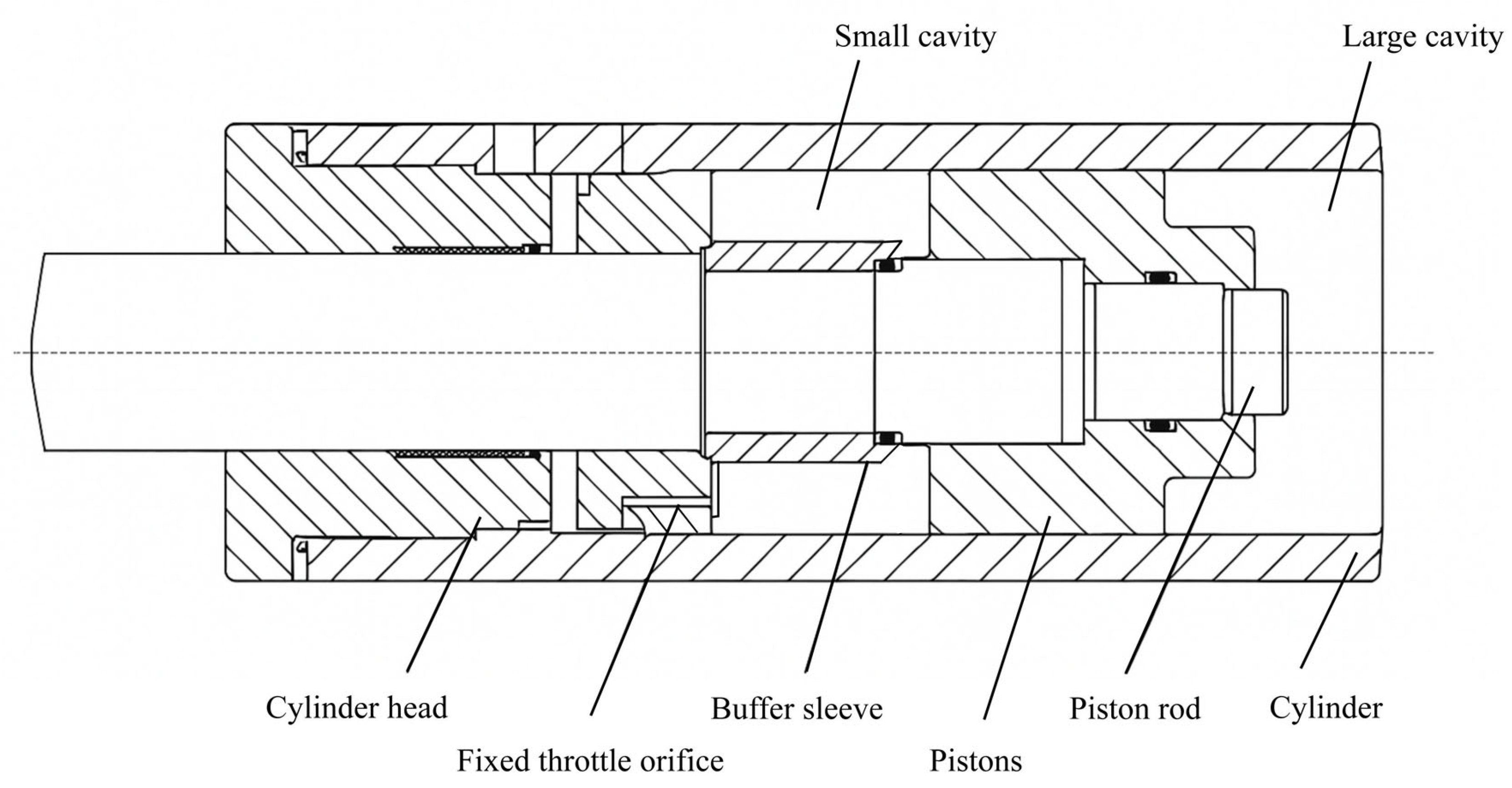
In the EHA system, in order to suppress the hydraulic shock caused by the end movement of the piston rod and to improve the stability and service life of the system, an integrated cushioning structure was designed on the side of the small cavity of the hydraulic cylinder, as shown in Figure 2. The structure mainly consists of the piston, piston rod, cylinder barrel, cylinder head, buffer sleeve, fixed throttle hole and other key components. As a movable throttle element, the buffer sleeve bears the important function of dynamically adjusting the flow resistance and realizing the end buffer in the process of system operation.

In the normal operating phase, that is, when the cushion is not open, the cushion sleeve is in a floating state, the hydraulic oil flows to the tank from the small cavity on the back side of the piston rod, and the flow path mainly relies on the channel inside the piston rod, which has a small resistance, and the system can achieve a fast response. When the piston rod is driven by hydraulic oil near the end of the stroke, the cushioning sleeve gradually moves forward and eventually fits with the cylinder head, and the hydraulic cylinder then enters the cushioning stage. At this stage, the original large through-flow channel is closed, and the discharge of hydraulic oil can only be completed through three restricted paths:

• The annular channel formed by the clearance between the buffer sleeve and the buffer hole of the cylinder block.
• The dynamically changing geometry of the flow path between the buffer sleeve and the buffer hole.
• The fixed throttle hole set in the cylinder head.

In the buffer process, the geometric relationship between the buffer sleeve and the buffer hole changes with its axial movement, making the cross-sectional area of the overflow gradually reduce. The throttling flow equation is shown in Equation (1).

$$Q=C_{d}A\sqrt{{\displaystyle \frac{2\Delta p}{\rho }}}$$

(1)

where Q denotes the volume flow rate (m³/s), C_d denotes the flow coefficient, the correction coefficient considering the shape of the throttle port, the flow state and other factors, A denotes the effective overflow area of the throttle port (m²), Δp denotes the pressure difference between the two ends of the throttle port (Pa), and ρ denotes the density of the fluid (kg/m³).

According to the throttling flow formula, it can be seen that the flow rate Q will decrease with the decrease of the overflow area A. The flow resistance increases, resulting in the slowing down of the hydraulic fluid flow rate. The increase in flow resistance leads to a slowdown in the flow rate of the hydraulic fluid and an increase in the back pressure in the small cavity, which in turn inhibits the speed of movement of the piston rod and achieves effective end cushioning control.

2.2. Simulation Model of EHA Hydraulic Cylinder Small Cavity Cushioning

According to Newton’s second law, the equilibrium equation of the hydraulic cylinder cushioning can be obtained as shown in Equation (2).

$$ma=p_1{A}_1-p_2{A}_2-{\beta }_{f}v-R_f-F$$

(2)

where m denotes the equivalent mass of the piston and load, a denotes the piston acceleration, p₁ denotes the large chamber pressure, A₁ denotes the large chamber area, p₂ denotes the cushion chamber pressure, A₂ denotes the cushion chamber area, ${\beta }_f$ denotes the coefficient of viscous friction, v denotes the piston speed, R_f denotes the coulomb friction, and F denotes the external load force.

According to the law of conservation of mass, the buffering process satisfies the continuity equation as shown in Equation (3).

$$Q_1=A_{2}v=C_d\pi d\delta \sqrt{{\displaystyle \frac{2}{\rho }}}{P}_1$$

(3)

where Q₁ denotes the buffer chamber flow rate, A₂ denotes the effective area of the buffer chamber, and v denotes the piston speed, C_d denotes the flow coefficient, d represents the buffer hole diameter, and $\rho$ indicates the fluid density. For the actual hydraulic oil used, $\rho$ = 850 kg/m³.

Combining Equations (2) and (3) yields Equation (4).

$${\displaystyle \frac{dV}{dt}}+K{V}^2-J=0$$

(4)

The formulas for the proportional coefficient K and the external drive J are shown in Equations (5) and (6).

$$K={\displaystyle \frac{\rho A_2^3}{2C_d^2\left(\pi d\delta \right)m}}$$

(5)

$$J={\displaystyle \frac{{\rho }_0{A}_0-F}{m}}$$

(6)

Solve the differential equation, considering that at t = 0, v = v₀, where v₀ is the initial velocity (m/s) upon entering the buffer. The final velocity formula for the piston buffer is given by Equation (7).

$$V=\sqrt{{\displaystyle \frac{J}{K}}}{\displaystyle \frac{\left(V_0+\sqrt{\frac{J}{K}}\right)e^{2\sqrt{JK}t}+\left(V_0-\sqrt{\frac{J}{K}}\right)}{\left(V_0+\sqrt{\frac{J}{K}}\right)e^{2\sqrt{JK}t}-\left(V_0-\sqrt{\frac{J}{K}}\right)}}$$

(7)

Differentiating Equation (7) yields the acceleration formula for the end of the piston buffer, as shown in Equation (8).

$$a=-{\displaystyle \frac{4J{e}^{2\sqrt{JK}t}\left(V_0^2-\frac{J}{K}\right)}{{\left[\left(V_0+\sqrt{\frac{J}{K}}\right)e^{2\sqrt{JK}t}-\left(V_0-\sqrt{\frac{J}{K}}\right)\right]}^2}}$$

(8)

At t = 0, the maximum negative acceleration $a=-\left(K{V}_0^2-J\right)$ is obtained. Substituting Equation (7) into Equation (3) yields the variation formula for the buffer chamber pressure P₁, as Equation (9).

$$P_1={\displaystyle \frac{\rho A_2^2}{2C_d^2{\left(\pi d\delta \right)}^2}}{V}^2$$

(9)

2.3. Mathematical Model of EHA Hydraulic Cylinder Small Cavity Cushioning

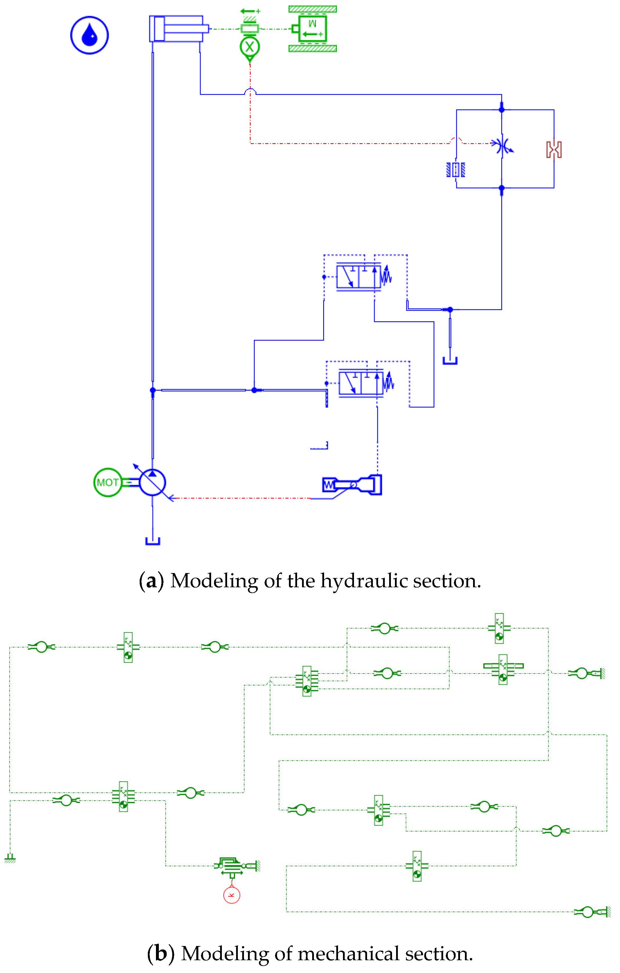
The EHA hydraulic cylinder small-cavity buffer simulation model is mainly composed of two major parts: the hydraulic system and the mechanical structure. Among them, the hydraulic system part includes components such as variable pumps, load-sensitive valves, pressure cut-off valves, hydraulic cylinder bodies, fixed dampers, variable dampers and key mating clearance structures in the buffer stage, aiming to accurately simulate the flow characteristics of the hydraulic fluid and its coupling effect with the buffer mechanism. The mechanical structure section is used to simulate the loads driven by the hydraulic cylinders in real life operation to assess the effect of cushioning performance on the end speed and impact response.

The simulation platform selects AMESim 2021 software for modeling and analysis and uses its library of Hydraulic Component Design (HCD), Hydraulics (HYD), signal control and mechanical system modules to complete the model construction [22]. The modules are coupled with each other through the energy and signal interfaces to build an integrated EHA hydraulic cylinder buffer simulation system. Figure 3 shows the complete model structure and its functional module division, which provides the basis for the subsequent dynamic response analysis and structural optimization.

3. Sensitivity Analysis of Buffer Structure Parameters

In order to study the influence of the key parameters of the buffer structure on the buffer performance of the hydraulic cylinder, this thesis selects four main structural parameters, namely, the clearance between the buffer sleeve and the buffer hole G, the diameter of the fixed throttling hole D, the angle of the wedge surface θ, and the length of the wedge surface L₁, and carries out the parameter sensitivity analysis. Among them, the fitting clearance G determines the ability of the hydraulic fluid to drain through the clearance during the cushioning stage, which directly affects the rate of energy release during the initial cushioning period. The fixed orifice diameter D controls the damping characteristics of the main relief channel, which in turn regulates the pressure build-up and decay characteristics of the cushioning process. The wedge angle θ and the length L₁ together determine the contact characteristics and the evolution of the oil channel during the cushioning process, and have a significant influence on the gradual closure of the cushioning chamber and the pressure surge. By comparing the dynamic response of the pressure change and piston speed in the buffer chamber under different parameter combinations, the influence degree and mechanism of each parameter on the buffer performance are systematically evaluated, which provides a theoretical basis and engineering reference for the optimal design of the buffer structure.

3.1. Influence of Fitting Clearance G on Cushioning Effect

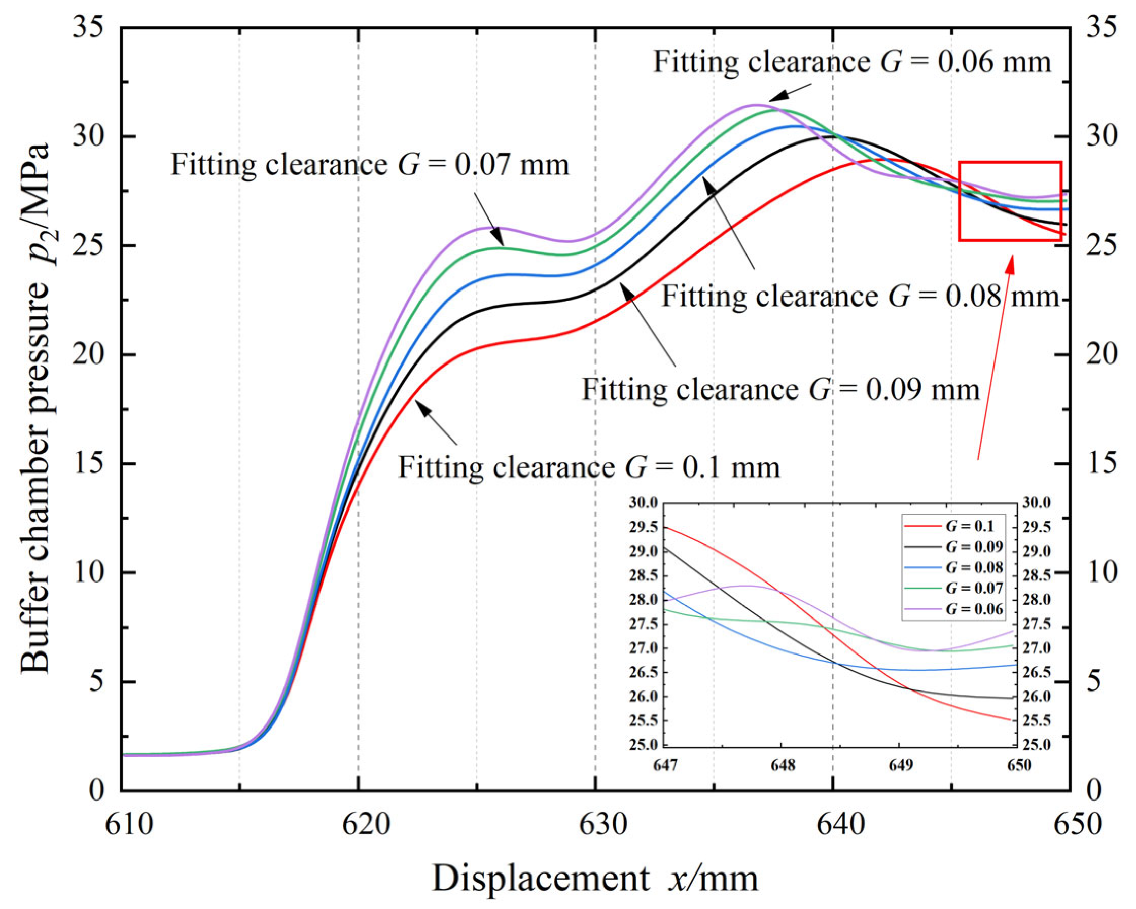
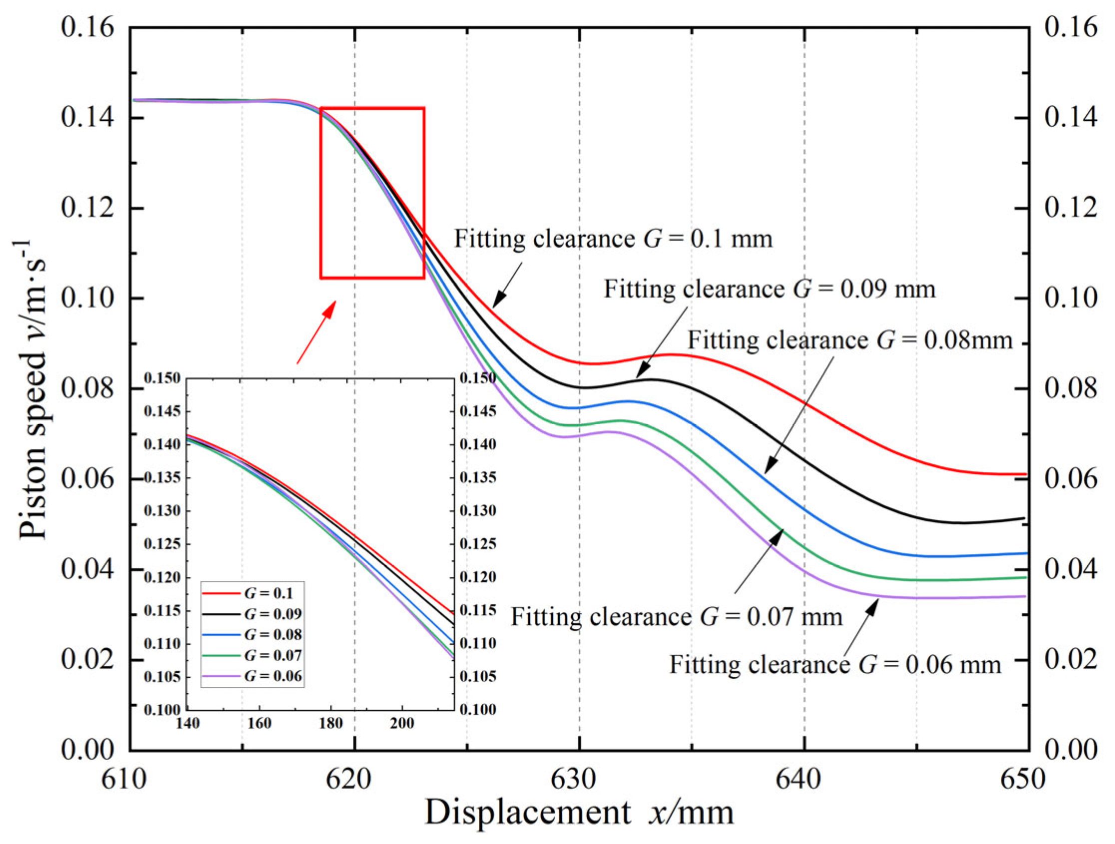
The fitting clearance G is a key parameter in the design of the EHA hydraulic cylinder cushioning structure, which has a significant effect on its cushioning performance. In order to study its action law, this thesis carried out a parameter sensitivity simulation analysis on the basis of fixing other structural parameters. The specific settings are: fixed throttle hole diameter D = 1.5 mm, wedge surface length L₁ = 36 mm, wedge surface angle θ = 0.6°, comparative simulation of the buffer structure under the conditions of different fitting clearance G, and the output of the corresponding displacement-buffer chamber pressure change curve and displacement-piston speed change curve, as shown in Figure 4 and Figure 5.

As shown in the Figure 4 and Figure 5, during the buffer process in the small chamber of the hydraulic cylinder, the size of the fitting clearance directly affects the oil discharge capacity by altering the effective flow area of the gap, thereby coupled to the buffer chamber pressure and the piston’s terminal speed. A smaller fitting clearance restricts oil discharge more severely, causing the buffer chamber pressure to rise faster. The peak and residual end pressures remain at higher levels, creating stronger throttling damping effects. This results in rapid speed decay after the piston enters the buffer zone, significantly reducing the terminal speed. Conversely, a larger fitting clearance reduces flow resistance, lowering the peak buffer chamber pressure and weakening the damping effect. This results in a relatively smoother deceleration process, lower terminal speed and increased terminal kinetic energy, potentially causing impact and whole-machine vibration. Simulation results indicate that a smaller clearance corresponds to higher peak pressure and lower terminal speed, while a larger clearance manifests as lower pressure and higher terminal speed. This indicates that buffer design must balance the risks of “excessive pressure causing structural and sealing hazards” against “excessive terminal speed leading to impact hazards.” Considering both pressure safety margins and terminal impact control requirements, a reasonable fitting clearance range should be maintained between 0.07 and 0.09 mm. This approach effectively reduces terminal speed while avoiding excessive peak pressure, thereby optimizing buffer performance.

3.2. Influence of Fixed Orifice Diameter D on Cushioning Effect

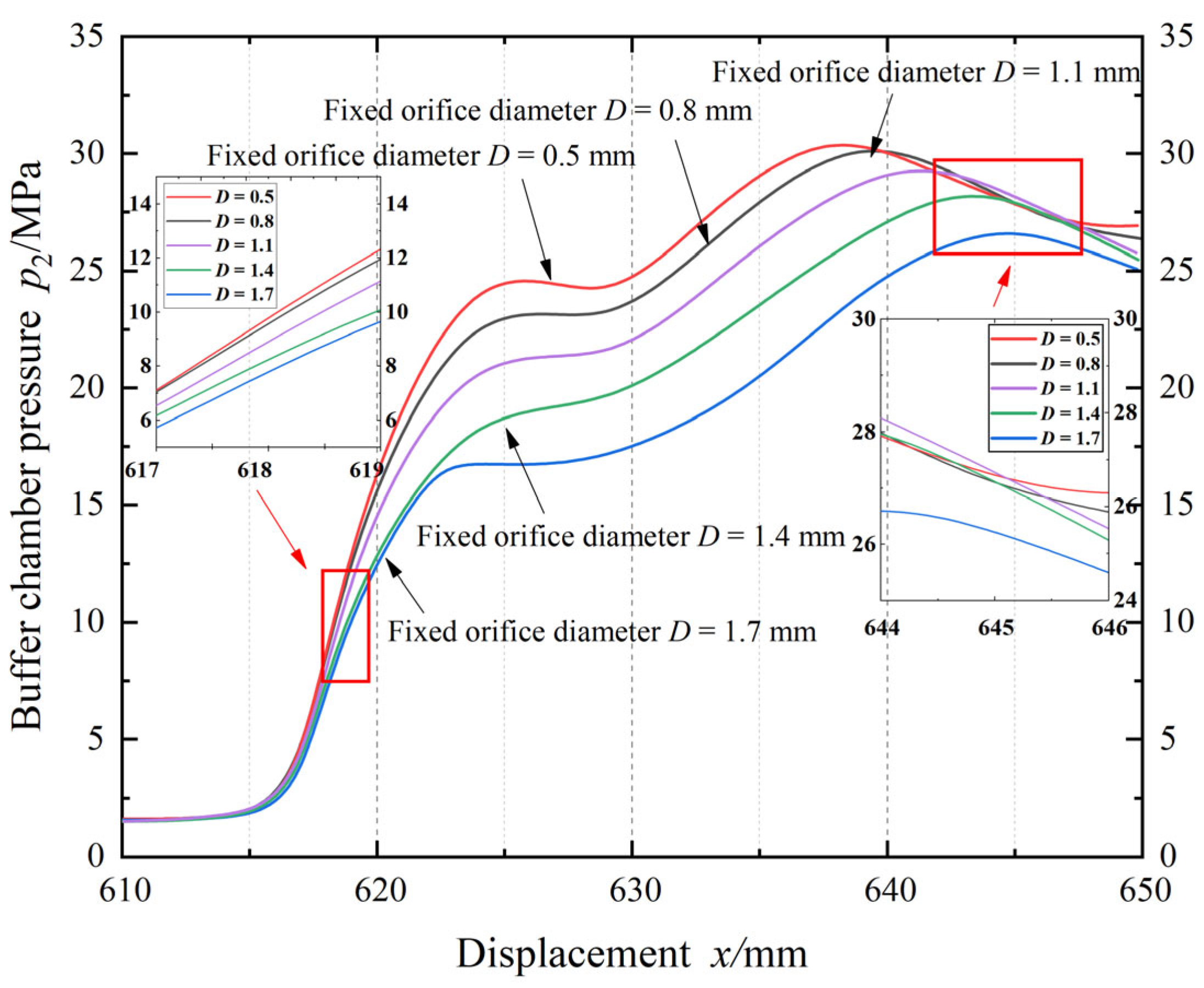
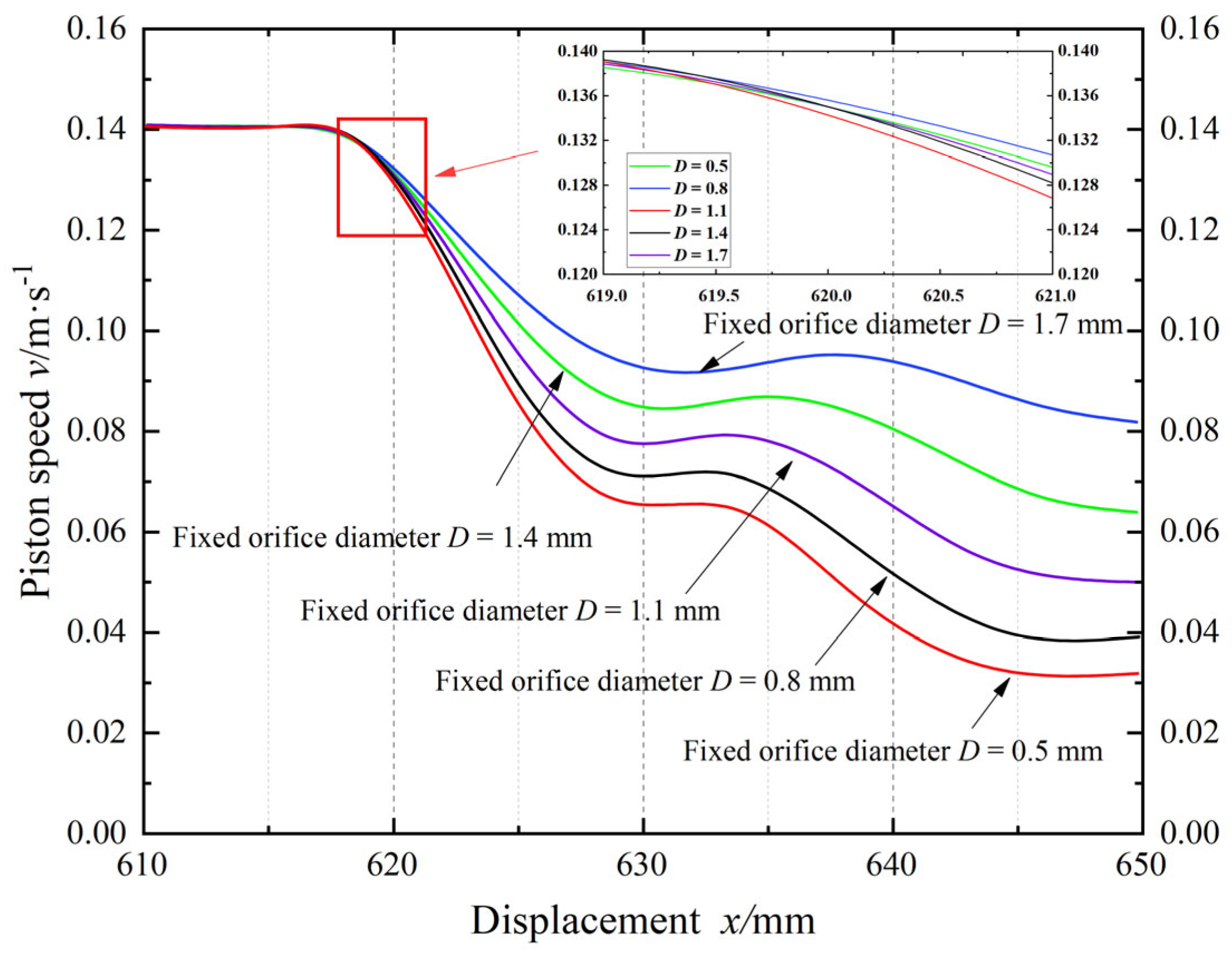
The fixed orifice diameter D is another key parameter in the design of the hydraulic cylinder cushioning structure, which has a direct influence on the energy dissipation and pressure regulation of the cushioning process. In order to investigate the law of action, simulation analysis is carried out in this thesis under the condition of keeping other structural parameters unchanged. The specific settings are: clearance G = 0.1 mm, wedge length L₁ = 36 mm, wedge angle θ = 0.6°, the buffer structure with different fixed throttle orifice diameter D is simulated, and the outputs of displacement-buffer chamber pressure change curves and displacement-piston speed change curves are output. The simulation results are shown in Figure 6 and Figure 7.

Simulation results indicate that the fixed throttle orifice diameter directly influences the pressure-velocity coupling characteristics during buffering by altering oil discharge capacity. Particularly in the latter half of the buffering stroke, the clearance flow area significantly diminishes, and oil discharge pathways become dominated by the throttle orifice. Consequently, its dimensions determine both the pressure build-up level within the chamber and the rate of piston kinetic energy dissipation. When the orifice diameter is small, oil discharge is restricted, leading to a marked increase in both the peak pressure and residual pressure at the end of the buffer stroke. This enhances damping effects, causing the piston speed to decay rapidly and achieve a lower terminal speed, thereby demonstrating strong buffering performance. However, excessively high pressure risks seal wear and structural stress exceeding permissible limits. Conversely, a larger orifice diameter facilitates smoother oil discharge, reduces pressure peaks and results in a more gradual deceleration process. This leads to higher terminal speeds, increasing the risk of impact and overall machine vibration. Figure 6 and Figure 7 reveal a high degree of consistency between the upward shift in the pressure curve and the steep decline in the speed curve, further validating the aforementioned causal relationship. Therefore, a balance must be achieved between cushioning strength and structural safety. An orifice diameter within the medium range can effectively suppress terminal speed while avoiding excessive pressure, thereby optimizing the integration of cushioning performance and system reliability.

3.3. Influence of Wedge Face Angle $\theta$ on Cushioning Effect

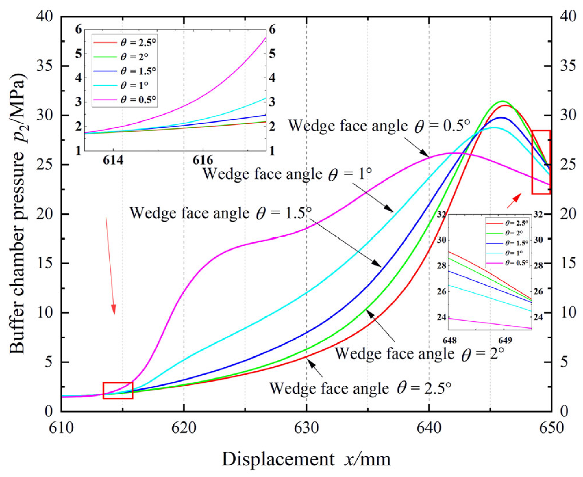
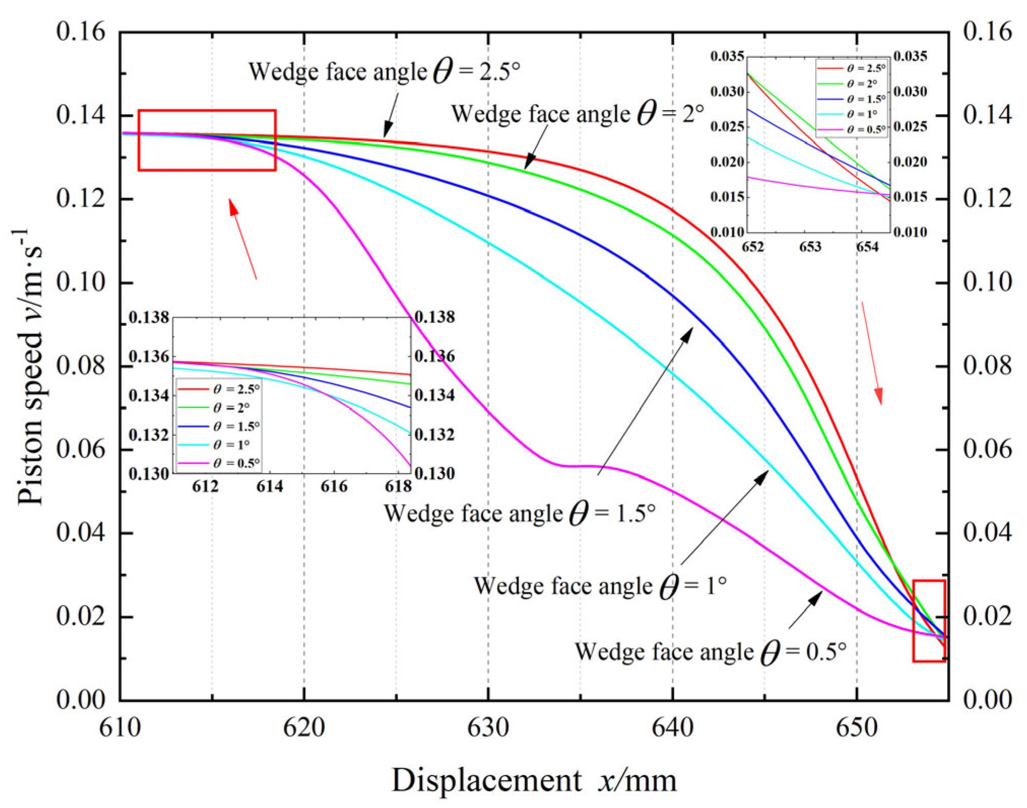
The wedge face angle $\theta$ is an important geometric parameter in the structural design of the cushion sleeve, which has a direct influence on the formation of the flow channel and the degree of oil restriction at the beginning of the cushioning phase. In order to analyze the specific role of the wedge face angle $\theta$ on the cushioning performance, simulation studies in this thesis are carried out under the condition that other structural parameters are kept constant. The specific settings are: fitting clearance G = 0.1 mm, fixed orifice diameter D = 1.5 mm, and wedge length L₁ = 36 mm under different wedge face angles of the buffer structure of comparative simulation, the output of the displacement-buffer cavity pressure change curve, and the displacement-piston speed change curve. The simulation results are shown in Figure 8 and Figure 9.

Combining Figure 8 and Figure 9 reveals that the wedge angle θ significantly influences the buffering process. Its primary mechanism lies in altering the rate at which the throttling area contracts with displacement, thereby directly regulating the timing and amplitude of cavity pressure establishment. Specifically, when θ = 0.5°, the throttling area changes slowly with displacement. Cavity pressure rises gradually only in the middle-to-late stages, resulting in the lowest pressure peak. This causes the piston to maintain high speed near the end stroke, leading to insufficient energy absorption during buffering. When θ increases to 1–1.5°, the throttling area contracts more rapidly, causing cavity pressure to rise sharply in the middle stroke. The pressure curve climbs smoothly with a moderate peak, while the speed curve exhibits a continuous monotonic decline. Terminal speed is significantly reduced with a more uniform deceleration distribution, achieving a favorable compromise between impact mitigation and smoothness. When θ further increases to 2–2.5°, cavity pressure builds earlier with a markedly higher peak. The pressure curve exhibits a steep rise near the end position, while the speed curve drops sharply at the end. Although the terminal velocity is lowest, indicating the most thorough kinetic energy absorption, the excessive deceleration gradient risks causing instantaneous impact forces and structural load peaks. In summary, increasing the wedge angle enhances cushioning effectiveness but simultaneously amplifies the risks of pressure peaks and abrupt speed changes. Therefore, a moderate θ (approximately 1.5°) achieves the optimal balance between terminal velocity control and cushioning smoothness, providing a rational parameter selection basis for design.

3.4. Influence of Wedge Face Length L₁ on Cushioning Effect

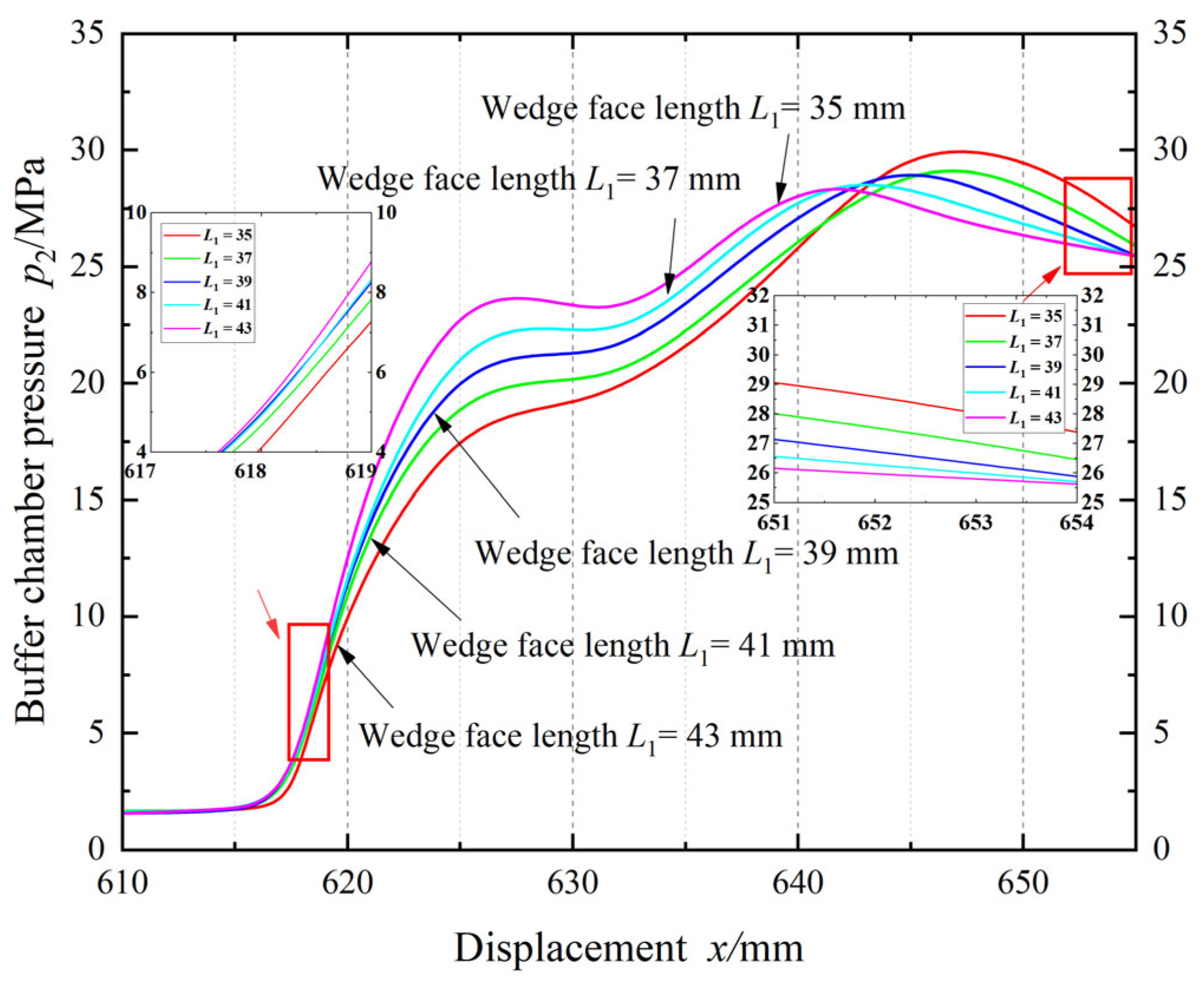
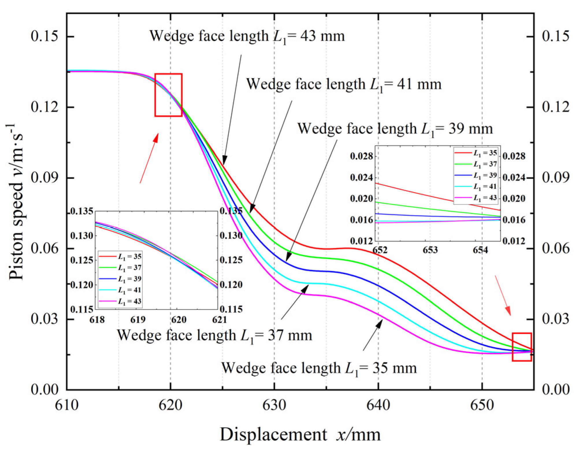
The wedge face length L₁ is one of the important parameters, indispensable to the design of the cushion sleeve structure, which directly determines the gradual process of the overflow channel in the cushioning stroke and has a significant impact on the regulation of the cushioning chamber fluid discharge path. In order to explore the influence of the length of the wedge face on the cushioning performance, this thesis carried out a comparative simulation analysis under the condition of keeping the other structural parameters constant. The specific settings were: fitting clearance G = 0.1 mm, fixed orifice diameter D = 1.5 mm, and a wedge face angle of 0.6°. Different wedge face lengths L₁ of the cushioning structure resulted in the output of the displacement-buffer chamber pressure change curves and displacement-piston speed change curves. The simulation results are shown in Figure 10 and Figure 11.

By combining Figure 10 and Figure 11, it can be seen that changes in the wedge surface length L₁ primarily affect the pressure build-up process in the buffer chamber and the piston deceleration characteristics by adjusting the rate of throttle area decay with displacement. When L₁ is short, such as 35 mm, the throttling area rapidly decreases within a short displacement range. This causes chamber pressure to surge rapidly during the initial cushioning phase, forming a higher peak pressure. Simultaneously, piston speed drops sharply, resulting in the lowest terminal velocity. This indicates the strongest kinetic energy absorption capability. However, excessive pressure gradients and abrupt deceleration changes may easily trigger structural impact and vibration risks. As L₁ increases to 39–41 mm, the cavity pressure rise becomes smoother, peak pressure moderately decreases and piston speed exhibits a gradual roll-off. Terminal velocity control is effective with uniform deceleration distribution, achieving a balance between adequate buffering and smoothness. When L₁ further increases to 43 mm, cavity pressure establishment is significantly delayed with a reduced peak. The piston speed reduction is insufficient, resulting in a high residual terminal velocity that weakens the buffer’s energy absorption capacity. This demonstrates that L₁ balances cushioning “stiffness” and “compliant flexibility.” A short L₁ emphasizes rapid deceleration but carries higher risks, while a long L₁ tends toward smoothness but insufficient cushioning. The optimal design range should be controlled between 39–41 mm to balance terminal speed reduction, controllable pressure peaks and stable deceleration, thereby achieving the best overall cushioning performance.

4. Predictive Modeling of Buffer Structures

In this section, an enhanced SBO–BP neural network prediction model is constructed and applied to predicting the performance of small-cavity buffer structures of EHA hydraulic cylinders. The BP neural network prediction model is enhanced by the introduction of an intelligent optimization algorithm, SBO, to improve the model’s ability to fit nonlinear dynamic characteristics and generalization performance [23]. Using the MATLAB platform, the complete process from data preprocessing and network design to model training and validation is realized, providing a theoretical basis for subsequent buffer performance optimization and parameter identification.

4.1. Hardware Configuration and Data Set Acquisition

In this thesis, the MATLAB R2023b platform was used to construct and train the enhanced BP neural network prediction model. The experimental hardware configuration used is shown in

Table 1. Experimental hardware configuration.

Hardware Components	Configure
CPU	Intel Core i7-12700H
RAM	16 GB DDR4
GPU	NVIDIA RTX 3050
SSD	512 GB NVMe SSD
Operating system	Windpws 10 64 bit

. This hardware configuration can effectively support the task of modeling, training, and performing predictive analyses of typical nonlinear systems such as EHA hydraulic cylinder small-cavity buffer structures with good computational performance and stability.

Through the sensitivity analysis of the EHA hydraulic cylinder small-cavity cushioning structure parameters in the third part of thesis, it can be seen that the key parameters affecting the end-piston speed include the fitting clearance G between the cushion sleeve and the cushion hole, the fixed orifice diameter D, the wedge face angle $\theta$, and the wedge face length L₁, which are taken as the input variables of the neural network model. A too-low buffer end speed will result in a long buffer time, which in turn affects efficiency. Therefore, the buffer time T (s), the end piston speed V_e ($\mathrm{mm}\cdot {\mathrm{s}}^{-1}$), the rate of change of the end piston speed V_r ($\mathrm{mm}\cdot {\mathrm{s}}^{-1}$), and the hydraulic oil return speed V_h ($\mathrm{mm}\cdot {\mathrm{s}}^{-1}$) are used as the output variables of the neural network.

Considering the process, equipment and other factors, the change range of the fitting clearance G is [0.05–0.1] (mm), and its change range is 0.01 mm as an interval. The fixed orifice diameter D can be altered in the range of [0.5–1] (mm) at intervals of 0.1 mm. The angle of the wedge face angle $\theta$ can be changed in intervals of 0.5° in the range of [0.5–3°] (angle). The length L₁ of the wedge face can be changed in [35–43] (mm) in 2 mm intervals. The above parameter combinations are brought into AMESim for simulation, and 36 sets of simulation data are obtained, of which the first 30 sets of data are the training set and the last six sets of data are the test set, as shown in

Table 2. Output value data for different buffer structure parameters.

x1 (G)	x2 (D)	x3 ($\mathit{\theta }$)	x4 (L1)	y1 (Ve)	y2 (T)	y3 (Vr)	y4 (Vh)
0.05	0.5	0.5	35	14.09	1.262	18.4297	16.908
0.05	0.6	1	37	16.32	1.141	23.214	19.584
0.05	0.7	1.5	39	18.92	1.029	29.2	22.704
0.05	0.8	2	41	21.84	0.929	39.88	26.208
0.05	0.9	2.5	43	25.35	0.841	52.8947	30.42
0.05	1	3	45	29.37	0.765	56.479	35.244
0.06	0.5	0.5	35	20.34	0.978	32.388	24.408
0.06	0.6	1	37	22.51	0.911	40.1515	27.012
0.06	0.7	1.5	39	25.16	0.845	50	30.192
0.06	0.8	2	41	28.26	0.783	58.1034	33.912
0.06	0.9	2.5	43	31.63	0.725	69.038	37.956
0.06	1	3	45	35.22	0.673	76.156	42.264
0.07	0.5	0.5	35	29.03	0.767	58.1081	34.836
0.07	0.6	1	37	31.18	0.73	66.2162	37.416
0.07	0.7	1.5	39	33.63	0.693	74.4737	40.356
0.07	0.8	2	41	36.46	0.655	86.4865	43.752
0.07	0.9	2.5	43	39.66	0.618	103.8235	47.592
0.07	1	3	45	43.19	0.584	116.27	51.828
0.08	0.5	0.5	35	39.74	0.616	100.5	47.688
0.08	0.6	1	37	41.75	0.596	102.1739	50.1
0.08	0.7	1.5	39	44.1	0.573	120.4545	52.92
0.08	0.8	2	41	46.75	0.551	129.5652	56.1
0.08	0.9	2.5	43	49.73	0.528	149.5454	59.676
0.08	1	3	45	53.02	0.506	156.4712	63.624
0.09	0.5	0.5	35	52.56	0.508	173.6363	63.072
0.09	0.6	1	37	54.47	0.497	177.6923	65.364
0.09	0.7	1.5	39	56.78	0.484	204.6154	68.136
0.09	0.8	2	41	59.44	0.471	235.3846	71.328
0.09	0.9	2.5	43	62.5	0.458	244.2857	75
0.09	1	3	45	65.92	0.444	259.3648	79.104
0.1	0.5	0.5	35	68.88	0.436	326.6666	82.656
0.1	0.6	1	37	70.84	0.43	334.2857	85.008
0.1	0.7	1.5	39	73.18	0.423	375.7143	87.816
0.1	0.8	2	41	75.81	0.416	415.7142	90.972
0.1	0.9	2.5	43	78.72	0.408	471.4286	94.464

.

Since the buffer structure parameters vary in order of magnitude, direct training leads to lower prediction accuracy of the prediction model. Therefore, this thesis normalized the buffer structure parameters to improve the efficiency and accuracy of the prediction model. The normalization process transforms the data into the interval [0, 1] as shown in Equation (10). The true predicted value of the model needs to be obtained by an inverse normalization process as shown in Equation (11).

$$x^{\ast }={\displaystyle \frac{x-x_{\min }}{x_{\max }-x_{\min }}}$$

(10)

$$z=z^{\ast }\times \left(x_{\max }-x_{\min }\right)+x_{\min }$$

(11)

where x is the original data; x_min is the minimum value of the original data; x_max is the maximum value of the original data; $x^{\ast }$ is the value after normalization of the original data; $z^{\ast }$ is the model predicted data; and z is the value after inverse normalization of the model predicted data.

4.2. The Social Behavior Optimization Algorithm

(1)

Introduction to the SBO algorithm

Social Behavior Optimization (SBO) is a novel group intelligence optimization method inspired by the human behavior of climbing the social ladder. The algorithm takes the individual self-improvement motivation as the core driving force and simulates the process of human beings in the social structure by imitating the elites, learning from successful experiences and iteratively improving their own behaviors so as to achieve an efficient search for the global optimal solution. The basic idea of SBO stems from research findings in cognitive science and behavioral economics, which show that humans, when faced with complex problems, tend to learn from individuals of higher social status or higher performance in order to improve their abilities. SBO formalizes this social learning mechanism as a computational model, constructing the optimization process through the framework of “elite demonstration + collective imitation”, reflecting an evolutionary mechanism analogous to that of mentoring and career paths in human societies.

In SBO, a “social network” is formed by sharing knowledge among intelligences, in which individuals gradually improve their “social status”, i.e., the value of the objective function, through observation, imitation and learning. During the operation of the algorithm, the strategies evolve naturally, creating a synergistic balance between exploration (searching for new opportunities) and exploitation (using the information already available) by different individuals. The working mechanism of SBO can be summarized in two main stages:

• Elite engagement phase (Exploration): In this phase, the agent focuses on the best-performing solutions in the current population and expands the depth of exploration in potential areas by steering the search direction. This process is equivalent to the individual seeking a mentor or role model in the social system through whom to enter a more efficient growth path.
• Resource acquisition and evaluation phase (Exploitation): Individuals take information from top-performing solutions and adapt and optimize their own solutions, similar to drawing on the experience of others in a professional field to improve one’s own competence. This phase strengthens the local development of the understanding and accelerates the convergence process.

SBO inherits and develops the basic ideas of the Human Behavior-Based Optimization (HBBO) approach [24]. HBBO usually simulates human social interaction behaviors such as imitation, collaboration and innovation, and is suitable for dynamically changing or multi-objective problems. Similarly, Educational Competition Optimizer (ECO) improves the overall population search quality by introducing a competitive learning environment in which individuals compete and learn around the optimal solution [25].

Compared with traditional group intelligence algorithms, SBO shows significant advantages in the following aspects:

• Achieving a more natural balance between global exploration and local exploitation enhances the ability of algorithms to leapfrog local optima;
• The sensitivity and debugging dependence on hyperparameters are drastically reduced and the portability and practicality of the algorithms are enhanced;
• Good scalability to adapt to the optimization needs of high-dimensional complex problems.

(2)

Mathematical modeling of SBO

$$X^1,X^2={\left[\begin{array}{c}{x}_1\\ ⋮\\ x_2\\ ⋮\\ x_3\end{array}\right]}_{N\times D}={\left[\begin{array}{ccccc}{x}_{1,1}& \dots & x_{1,j}& \dots & x_{1,D}\\ ⋮& \ddots & ⋮& \ddots & ⋮\\ x_{i,1}& \dots & x_{i,j}& \dots & x_{i,D}\\ ⋮& \ddots & ⋮& \ddots & ⋮\\ x_{N,1}& \dots & x_{N,j}& \dots & x_{N,D}\end{array}\right]}_{N\times D}$$

(12)

In the initialization phase of the enhanced Social Behavior Optimization algorithm, a two-population design strategy is introduced to enhance population diversity and improve search efficiency. Specifically, as shown in Equation (12), two independent but corresponding populations X¹ and X² are constructed, where each population contains N individuals with index i ∈ {1, 2, …, N} corresponding to members of the same household. In this design, X¹(i) and X²(i) represent individuals with different levels of knowledge and social status in the i-th family, thus reflecting the heterogeneity and behavioral diversity within the family at the initialization stage.

Each individual’s state is shown in Equation (13):

$$x_{i,j}=U\left(l{b}_j,u{b}_j\right)$$

(13)

where x_i,j is the j-th decision variable for the i-th individual, D is the number of decision variables, and lb_j and ub_j are the upper and lower bounds, respectively. This uniform initialization of the N × D matrices of the two populations establishes the dimensional nature of the problem and ensures different starting points.

After initialization, the selection process identifies the elite members of each household to form the elite population X_e. Specifically, for household i, the selection of the elite scheme is shown in Equation (14).

$$x_i^e=\left\{\begin{array}{cc}{x}_i^1& fobj\left(x_i^1\right)<fobj\left(x_i^2\right)\\ x_i^2& otherwise\end{array}\right.$$

(14)

where $fobj\left(\cdot \right)$ is the objective function.

The two-population structure improves the algorithm’s coverage and global exploration ability in the search space by introducing role differences (common versus elite individuals) and information polygraphy, providing guarantees for convergence and robustness [26]. The structure not only facilitates the implementation of the elite selection and learning renewal mechanism but also simulates the status-based social interaction and resource sharing mechanism in a real society, reflecting the role of individual strengths and strategic connections in social progress.

In the elite engagement phase, the SBO algorithm draws on the dynamic evolution mechanism of status structure in human societies to enhance the efficiency of deep mining and exploration of optimal solutions. This stage accelerates the progress of ordinary individuals by simulating the process of individuals actively seeking guidance from high-status mentors (i.e., elite individuals in the algorithm), which embodies the characteristics of information flow and resource sharing across families, thus breaking through the limitations posed by the traditional isolated-family framework and constructing a more adaptive and robust search mechanism.

For the specific implementation, the SBO algorithm uses a roulette wheel selection strategy [27,28,29] to randomly select representative individuals from a candidate subset consisting of the best-performing individuals in each family. This probabilistic selection approach avoids the reliance on a single elite and enhances the diversity and depth of exploration of the algorithm while reflecting the nonlinear, strategic and uncertain characteristics of human social networks.

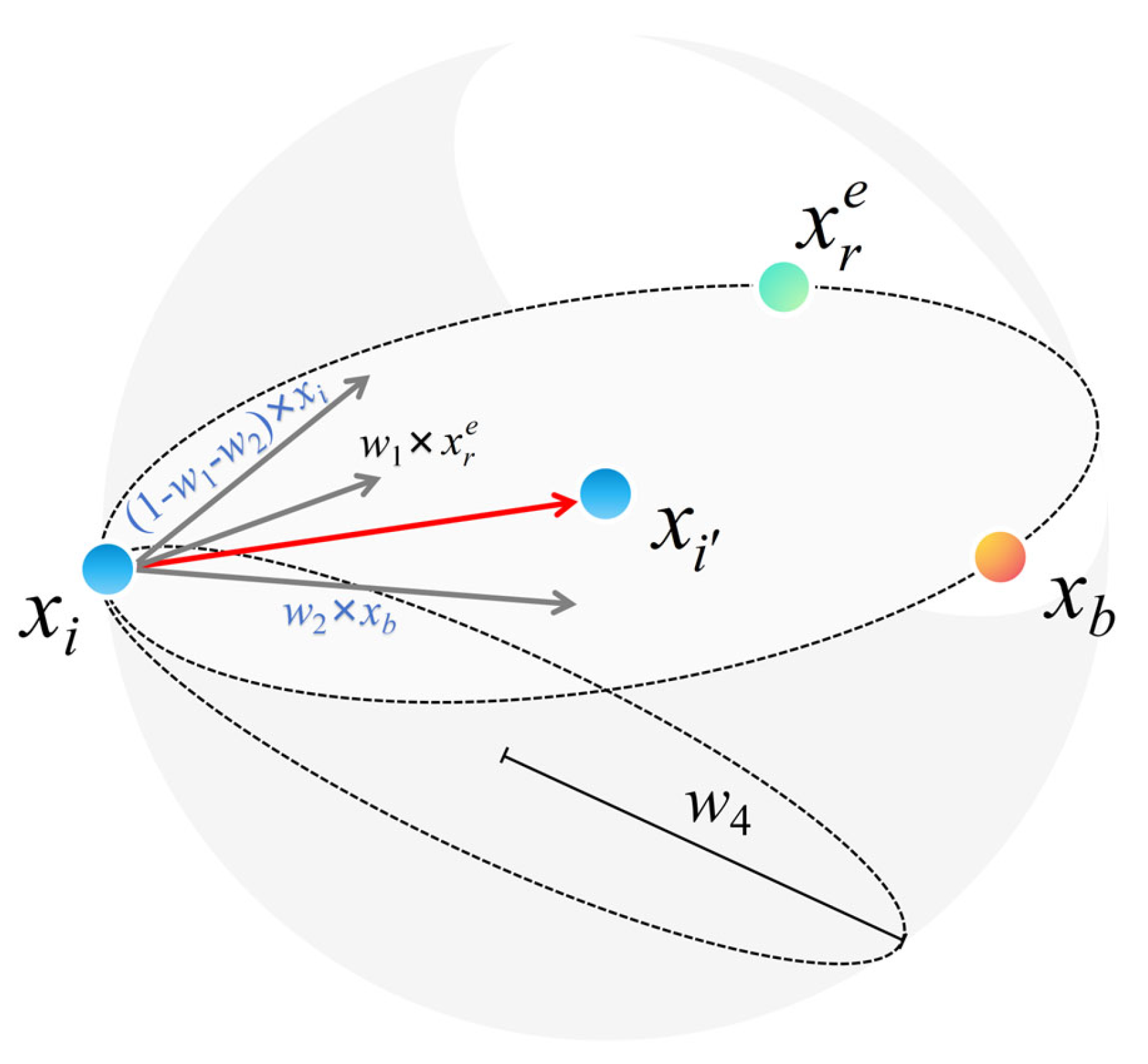
The selected elite individual $x_i^e$, together with the optimal solution x_b in the current population, forms a high-status search circle, which corresponds to a region of potential optimization value in the solution space and guides the other individuals to cluster toward the better solution. This type of social mobility modeling mechanism effectively facilitates the migration of individuals from the current region to more promising solution spaces, thus improving the overall search efficiency and convergence performance of the algorithm.

To mathematically model this behavior, Figure 12 illustrates the generation process of an individual x_i within a high-status circle, thus defining a committed region in the space of understanding, whose mathematical form is described by Equation (15). This high-status circle constitutes an adaptive region in the space of understanding, within which the individual performs guided searches aimed at achieving an effective balance between structural evolution and exploratory perturbations. In this framework, the behavioral evolution of an individual is driven by several key factors, and its positional update mechanism reflects the intention to converge to a high-quality solution while retaining a certain degree of randomness to avoid falling into a local optimum. This modeling approach not only improves the orientation of the search process, but also enhances the coverage of the solution space, thus contributing to the overall optimization performance.

$$x_{i^{\prime }}=\left\{\begin{array}{cc}\left(1-w_1-w_2\right)\times x_i+w_1\times x_r^e+w_2\times x_b& \mathrm{rand}<w_3\\ w_4\times \left(\left(1-w_1-w_2\right)\times x_i+w_1\times x_r^e+w_2\times x_b\right)& otherwise\end{array}\right.$$

(15)

where x_i denotes the i-th individual in the population, $x_{i^{\prime }}$ denotes the next iteration, which is an elite individual selected from the random number population by the roulette method, and x_b is the best solution found so far. The movement strategy in Equation (15) ensures that individuals are influenced by their location, their high-performing peers and the best-known solution.

The parameters w₁ and w₂ are generated using randn to provide normally distributed randomness to weight the contributions of x_i, $x_i^e$ and x_b. These values introduce randomness while ensuring that moves remain within logical limits, facilitating a controlled but varied search in the solution space. The parameters w₃ and w₄ are used as adjustable design variables to dynamically balance the effect of the high state circle on the global exploration and local mining behaviors in the algorithm, aiming to improve the adaptability and convergence performance of the algorithm, where w₃ is shown in Equation (16).

$$w_3=\tanh \left({\left({\displaystyle \frac{\sqrt{\left|MaxFEs-\mathrm{randn}\times FEs\right|}}{i}}\right)}^{{\displaystyle \frac{FEs}{MaxFEs}}}\right)$$

(16)

where MaxFEs denotes the maximum number of function evaluations, FEs is the current number of evaluations that have been performed, and i is the individual index. This formula realizes an adaptive trade-off between the standard updating mechanism and the stochastic search strategy by dynamically adjusting the value of w₃ along with the optimization process, so as to flexibly regulate the extent of global exploration and local exploitation at different stages.

If rand ≥ w₃, Equation (17), where w₄ is used as a scaling factor, is used to generate uniformly distributed random numbers between [−w₃, w₃]. This mechanism increases exploration diversity by enabling step-size adjustment, especially when escaping local optima.

$$w_4=\mathit{unifrnd}\left(-w_3,w_3\right)$$

(17)

By integrating structured learning mechanisms with exploratory flexibility, the SBO algorithm simulates the decision-making behavior of real-world individuals who actively explore unconventional paths to achieve optimal outcomes while pursuing successful paradigms. In particular, Equation (15) strategically calculates the optimal position in high-status circles, reflecting the process by which an individual acquires better development prospects with the help of a network of influence. As the evolutionary process advances, the solution gradually approaches more promising regions in the search space, achieving successive optimization. Meanwhile, another update formula introduces a random scaling factor w₄ defined in the interval [−w₃, w₃], which enables the algorithm to jump out of the current search region while exploring the locally optimal solution, effectively suppressing the risk of the algorithm falling into the local optimum and improving the ability of global exploration of the solution space. This mechanism reflects the behavioral characteristics of human beings who actively deviate from the mainstream path and explore potential opportunities in the decision-making process. In summary, the SBO algorithm achieves a dynamic balance between exploitative and exploratory search, which not only improves the global quality of the solution and the optimization efficiency, but also has good problem adaptability and robustness, showing excellent performance in complex optimization tasks.

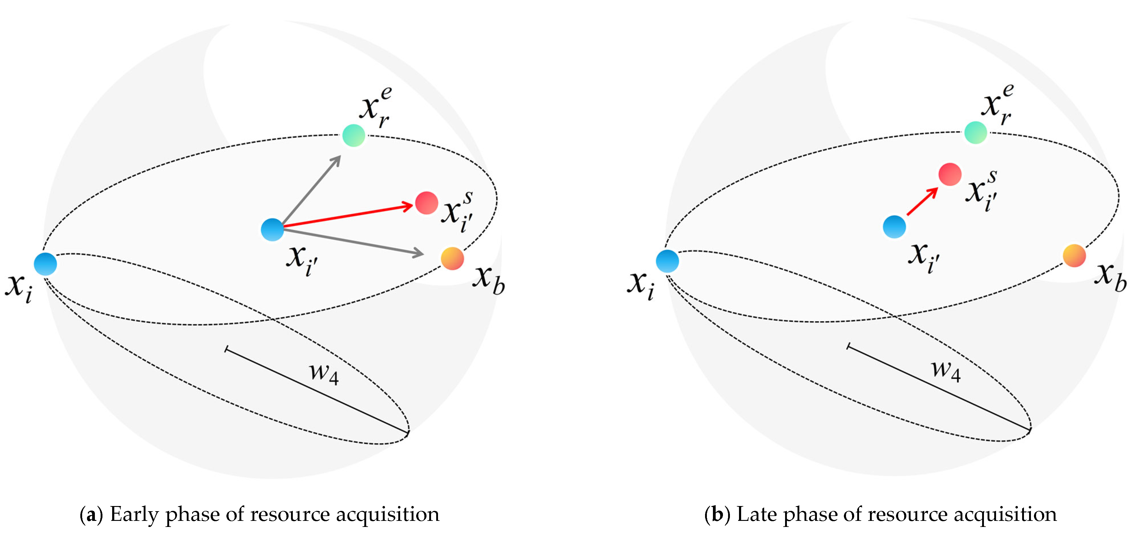
In the resource acquisition phase, individuals play a key role in the transition from exploration to exploitation by acquiring and integrating valuable information resources (similar to social capital) from their social networks. This phase begins by assigning all individuals in population X a flag vector, initialized to 1, as their initial success flag associated with the current state. This marker will be dynamically updated in subsequent resource assessment phases to reflect an individual’s performance in terms of efficacy as the status evolves.

The strategic mechanisms of resource acquisition are differentiated by the social status of the individual. For individuals in high social status, their resource integration process shows more selectivity, acquiring resources from two key sources of information: one originating from another high-status member within the same family unit, and the other from the best-performing individual in the group as a whole, as shown in Equation (18).

$$x_{i,j_1}^s={\displaystyle \frac{x_{i,j_2}^e+x_{b,j_3}}{2}}$$

(18)

where j_idx = randi(D), where idx = 1, 2, 3, reflecting the mix of family and external elite influence. By providing a balanced blend of these two sources, the algorithm guides high-status individuals to make more strategic resource allocations based on leveraging the strengths of their networks, thereby enhancing their optimization capabilities and search efficiency.

On the other end of the social scale, unsuccessful socializers have to rely on family resources. Their resources are updated as shown in Equation (19).

$$\begin{array}{cc}{x}_{i,j}^s=x_{i,j}^e& m_j\end{array}=1$$

(19)

where the row vector m is initially zero and is updated by Equation (20) prior to the social interaction.

$$m\left(u\left(1:\mathrm{ceil}\left(\mathrm{rand}\times D\right)\right)\right)=1$$

(20)

where u = randperm (D), provides a random permutation of the decision variable indexes.

As shown in Figure 13, the resource acquisition phase directs the clustering of populations toward more promising areas in the solution space through a status-driven differential renewal strategy, thus enhancing the exploitability and utilization efficiency of the solution. Figure 13a depicts that the top-performing individuals in the society optimize their location with the help of resources from high-status agent individuals, improving their local search accuracy through the introduction of external high-quality information. On the other hand, Figure 13b demonstrates that the disadvantaged individual relies on familiar family resources for self-reorientation, attempting to find a path of improvement in a known environment. This mechanism reflects individual heterogeneity in resource integration and location updating strategies driven by social hierarchies. It also promotes effective synergy between exploration and exploitation for the overall population.

In the resource evaluation phase, the SBO algorithm determines the effectiveness of the resources acquired by the individual, aiming to assess whether the integration of resources positively affects the individual’s fitness (i.e., “health status”). This stage is based on the initialized marker vector, where “1” indicates an improvement in fitness (i.e., successful assessment), while “0” indicates no improvement in fitness (unsuccessful assessment), thus tracking and recording the evolutionary process of the individual. This enables the tracking and recording of the evolutionary process of an individual.

Specifically, if the objective function value of the updated individual $x_i^s$ is better than that of the original x_i, the new state is retained, as shown in Equation (21).

$$\begin{array}{cc}{x}_i=x_i^s& \mathit{fobj}(x_i^s)\end{array}<\mathit{fobj}(x_i)$$

(21)

At the same time, we refresh the flag vector as shown in Equation (22).

$$fla{g}_i=\left\{\begin{array}{cc}1& \mathit{fobj}\left(x_i^s\right)<\mathit{fobj}\left(x_i\right)\\ 0& otherwise\end{array}\right.$$

(22)

Individuals who do not progress will remain in their current position while successful individuals will move to a superior position. This selective process reflects real-world social progress, where only valuable resources, those that clearly improve an agent’s position, are retained. This mechanism ensures the algorithm’s selective retention strategy after resource utilization, effectively improving the quality of understanding and the stability of the optimization process.

When the algorithm meets the termination conditions (e.g., reaches the maximum number of function evaluations or obtains an optimized solution validated by an augmented metric), it enters the integration phase. Until then, the algorithm cycles through the core mechanisms of “elite participation”, “resource acquisition”, and “resource evaluation” to continuously improve the population’s adaptation through state-driven interactions. In the consolidation phase, the algorithm extracts and generates the final solution reflecting the state evolution process based on the compilation of the objective function and the historical evaluation results, ensuring efficient resource allocation and forming structured analysis reports and application documents to support the interpretability of the solution and subsequent deployment requirements. This stage not only marks the end of the optimization process but also demonstrates the effective synergy and convergence of the algorithm between global exploration and local development.

The complete implementation framework of the SBO algorithm and the pseudo-code of the algorithm are shown in Algorithm 1.

Algorithm 1. Pseudo-code for the SBO algorithm

SBO Algorithm Pseudo-Code

Input: N, D, MaxFEs, lb, ub, fobj

Output: xb

1   Initialization:

2             Initialize X, Xe, Fitting, Fite, flag

3             Calculate Fitting and Fite

4             Update Xe and xb

5        while FEs < MaxFEs do

6             Select $x_r^e$ from Xe by Roulette Wheel

7             Elite Engagement:

8                   Update w1, w2, w3, w4

9                   Update X by Equation (9)

10                Apply Boundary control to X

11                Initialize Xs as X

12           Resource Acquisition:

13                Initialize row vector m as 0

14                Update m by Equation (14)

15                foreach xs ∈ Xs do

16                     if xs is successful then

17                          Updata xs by Equation (12)

18                     else

19                          Update xs by Equation (13)

20           Resource Evaluation:

21                Update X by Equation (15)

22                Update flag by Equation (16)

23           Consolidation:

24                Update Xe and xb

25                FEs → FEs +2N

The computational complexity of the enhanced SBO algorithm is O(T⋅N⋅(F + D)), where T is the number of iterations, N is the population size, D is the problem dimension, and F is the cost of the fitness function evaluation. This indicates that the overall complexity scales linearly with the population size and number of iterations, making SBO computationally efficient for high-dimensional problems.

4.3. SBO–BP Neural Network Prediction Model

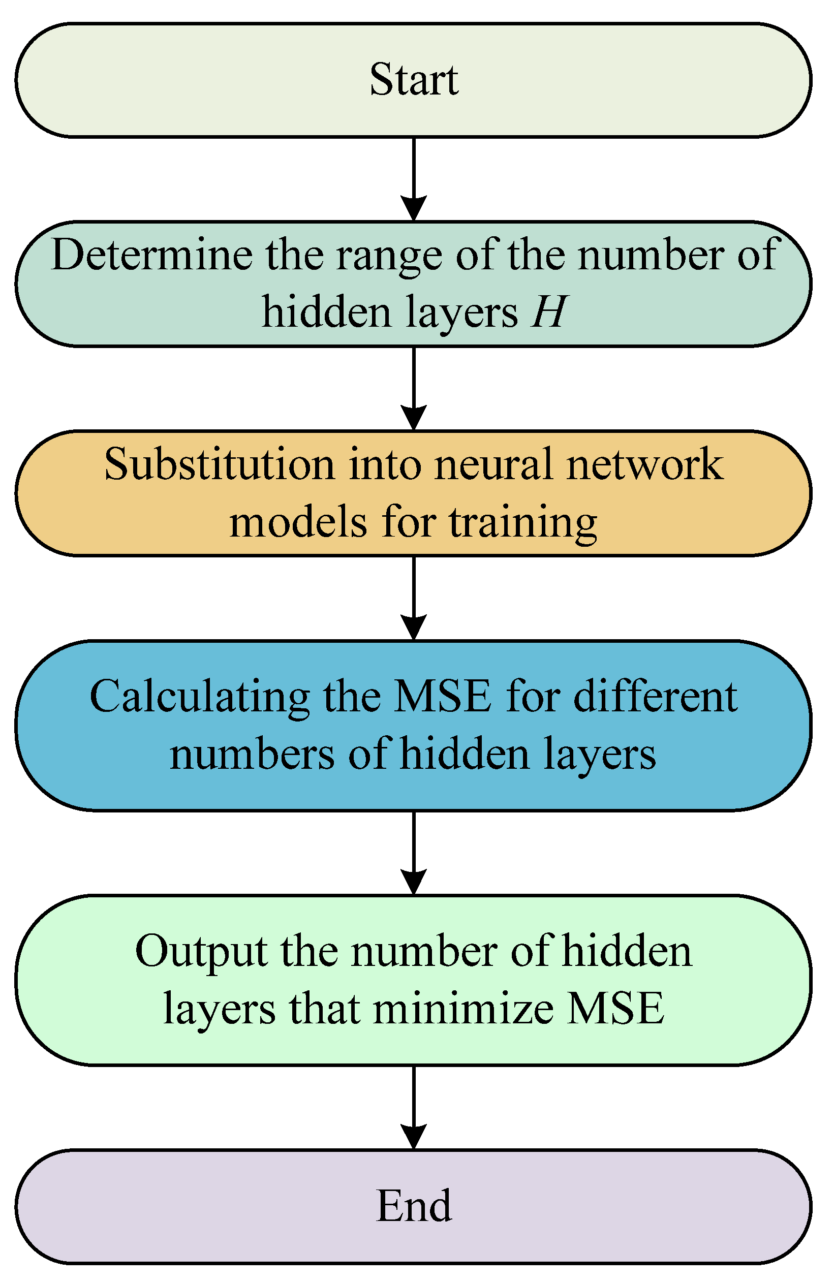
In the process of constructing the SBO–BP neural network prediction model, in order to determine the optimal number of hidden layers in the network structure, this thesis sets a reasonable range for the number of hidden layers based on Equation (23) and conducts layer-by-layer testing by means of loop iteration. Specifically, for each candidate number of layers, the neural network model is constructed and trained separately, and its corresponding mean square error (MSE) is recorded as the performance evaluation index. The number of hidden layer layers that minimizes the mean square error is finally selected as the optimal structure of the model, and the test results of this process are shown in Figure 14.

$$H=\sqrt{M+P}+a$$

(23)

where H is the number of hidden layers, M is the number of input layers, P is the number of output layers and a is an integer between [1, 10].

In terms of determining the network hyperparameters, the final number of hidden layers selected in this thesis is 10, and the number of training times is set to 1000 to ensure that the model has sufficient learning capability. In terms of learning rate, it is set to 0.001 to balance the training convergence speed and stability. The training accuracy threshold is also set to 1 × 10⁻⁶ to meet the high demand for prediction accuracy.

In order to improve the accuracy and generalization ability of the BP neural network prediction model, this thesis introduces the enhanced SBO algorithm to globally optimize the initial weights and thresholds of the BP neural network so as to overcome the problems of the traditional BP algorithm, which is prone to slow convergence speeds falling into the local minima during the training process. In order to verify the effectiveness and advantages of the SBO algorithm in parameter optimization, a variety of newly proposed intelligent optimization algorithms with excellent performance after 2023 were selected as the comparison algorithms in this thesis, such as the Newton-Raphson-Based Optimizer (NRBO, 2024) [30], GOOSE algorithm (GOOSE, 2024) [31], Chinese pangolin optimizer (CPO, 2025) [32], Snow ablation optimizer (SAO, 2023) [33], and Enzyme Action Optimizer (EAO, 2024) [34]. Control tests were conducted based on the same network structure with experimental data. To ensure the fairness and scientific validity of the comparison experiments, all optimization algorithms were tested against each other in the experiments using a unified network structure, dataset division and evaluation index system, in which the population size was 50 and the maximum number of iterations was 200.

The convergence trend of the iterative process is shown in Figure 15, which visually reflects the differences between the algorithms in terms of convergence speed and global search ability in optimizing the weights and thresholds of the BP neural network structure. The results show that all the algorithms show a certain convergence ability at the beginning of the iteration, but there are obvious differences in the convergence speed and the final adaptation value. The SBO algorithm reaches a lower fitness value within the first 30 iterations, indicating that it has a stronger initial global exploration capability. In the later stage of convergence, the fitness value of SBO continues to converge to 0.0061, which is better than the remaining five algorithms, reflecting its advantages in terms of optimization accuracy and stability. In contrast, CPO and GOOSE have slightly lower final convergence accuracies, although they also show a faster decreasing trend in the initial stage, while NRBO, SAO and EAO have lower decreasing rates and final performances than SBO, showing that their optimization capabilities are relatively limited. In summary, SBO shows better performance in both the convergence speed and quality of the solution, which further verifies the performance advantage of the SBO algorithm in optimizing the structure of BP neural networks, and provides an effective support for the construction of the high-precision prediction model SBO–BP.

As shown in

Table 3. Experimental hardware configuration.

Algorithm	Initial Fitness Value	Final Fitness Value	Final Ranking
NRBO (Black)	0.4057	0.01385	3rd
GOOSE (Magenta)	0.4366	0.00954	4th
CPO (Green)	0.4286	0.00705	2nd
SAO (Blue)	0.5012	0.01791	6th
EAO (Cyan)	0.3879	0.00744	5th
SBO (Red)	0.4817	0.00614	1st

, all six algorithms exhibit a clear decreasing trend in fitness value, indicating their effectiveness in solving the optimization problem. Among them, the SBO algorithm achieves the best final performance with a fitness value of 0.00614, ranking first in accuracy. Although its initial value is relatively high (0.4817), SBO converges rapidly and outperforms all other methods. CPO also shows competitive results, with a low final fitness value of 0.00705, ranking second. In contrast, SAO starts with the highest initial value (0.5012) and converges the slowest, resulting in the worst final performance (0.01791), likely due to premature convergence or local optima. GOOSE and NRBO achieve moderate results, while EAO demonstrates stable but less competitive performance. These results suggest that SBO is particularly well-suited for high-precision, nonlinear multi-objective optimization problems, validating its integration with NSGA-II for enhanced global search capability and solution diversity.

4.4. SBO–BP Neural Network Model Prediction Results

In this thesis, the prediction performance of the SBO–BP neural network model is comprehensively evaluated by training test comparison plots, linear fitting plots, regression plots and error histograms.

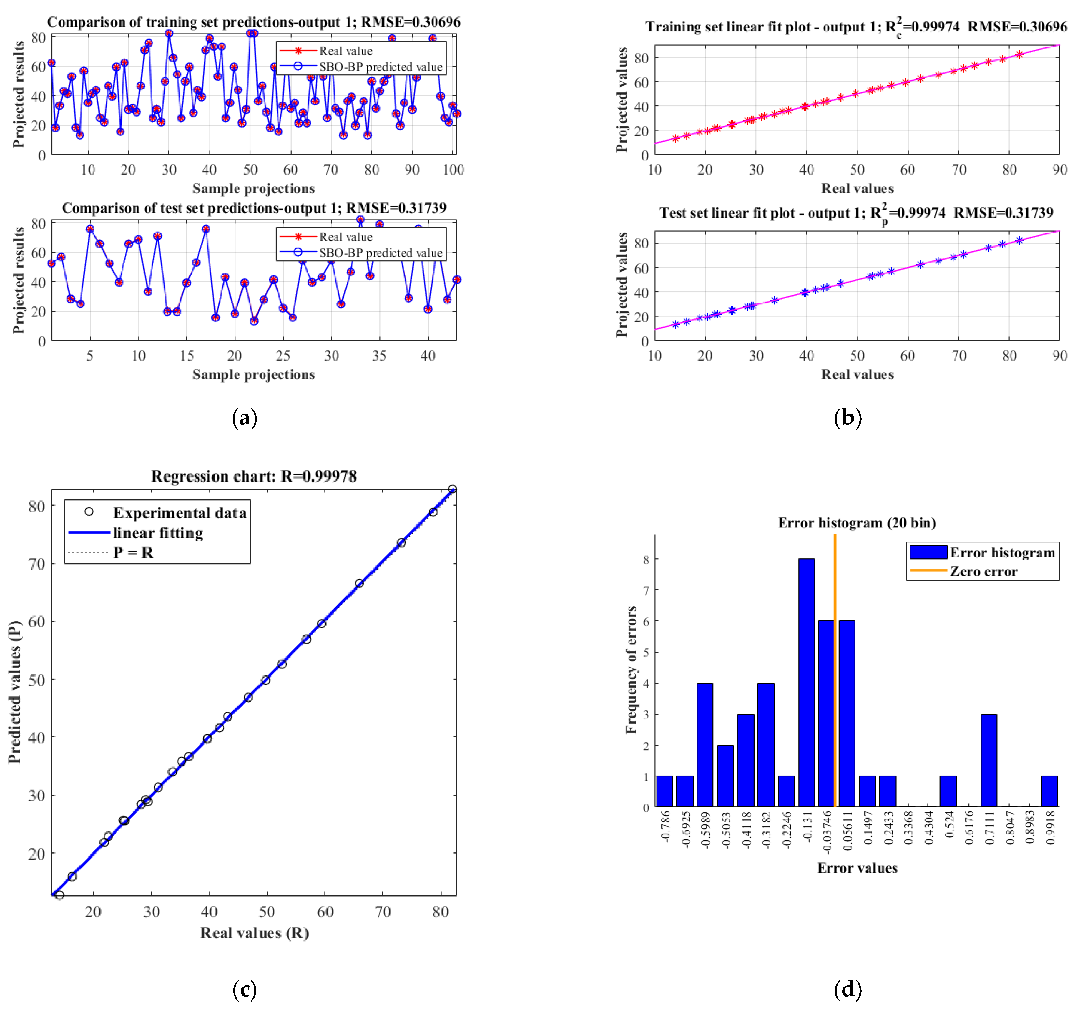
First, the predicted values of end-of-piston speed V_e for the test set were experimentally compared with the AMESim simulation values, as shown in Figure 16. The results show that the RMSE of the model on the training set and test set were 0.30696 and 0.31739, respectively, and the predicted values are more consistent with the AMESim simulation values. The correlation coefficient in the regression plot reaches 0.99978, indicating a strong linear correlation between the predicted results and the true values. The R-Square (R²) of both training and testing in the linear fitting plot is 0.99974, which further verifies the fitting accuracy. The error histogram shows that most of the errors are concentrated in the interval close to zero, indicating small model errors and strong prediction stability.

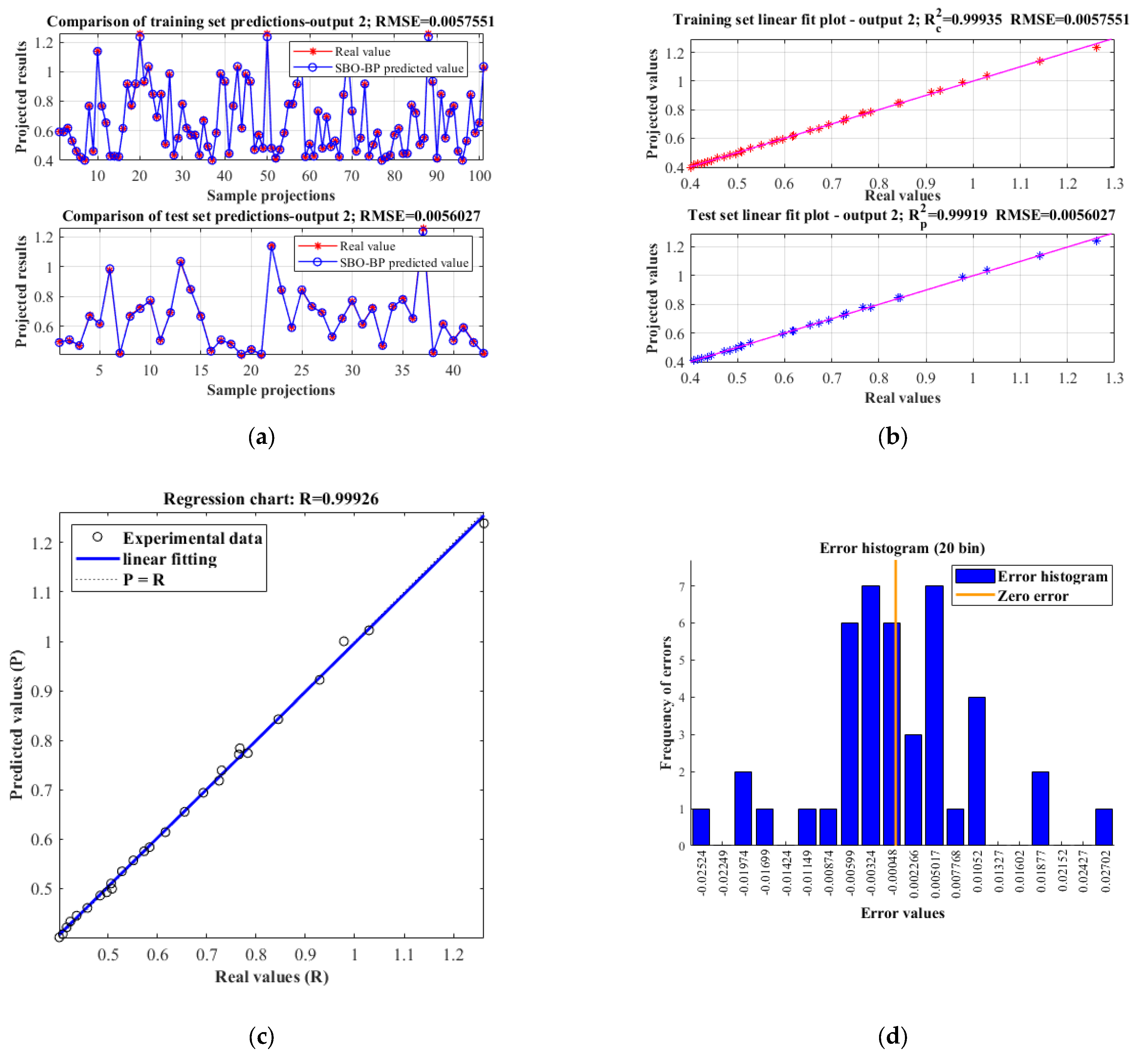
Second, in order to verify the accuracy of the SBO–BP neural network model in the task of buffer time T prediction, we conducted a modeling prediction and error analysis on the second set of outputs, as shown in Figure 17. From the prediction comparison plots of the training set and the test set, the model predictions highly overlap with the AMESim simulation values, with RMSEs of 0.0057551 and 0.0056027, respectively, indicating that the model maintains high prediction accuracies on different datasets. In the regression plot, the data points are highly distributed along the ideal fitting line (P = R) with a correlation coefficient R² = 0.99926, reflecting an extremely strong linear correlation between the model output and the actual values. In the linear fitting plots, the coefficients of determination of the training and test sets are ${\mathrm{R}}_c^2$ = 0.99935 and ${\mathrm{R}}_p^2$ = 0.99919, respectively, and the fitting curves are almost overlapped with the ideal fitting line, which further proves that the model has superior fitting ability and generalization performance. The error histogram shows that most of the errors are concentrated in the range of [−0.004, 0.004], showing a symmetric distribution, and the very small error values indicate that the prediction results have strong consistency and stability.

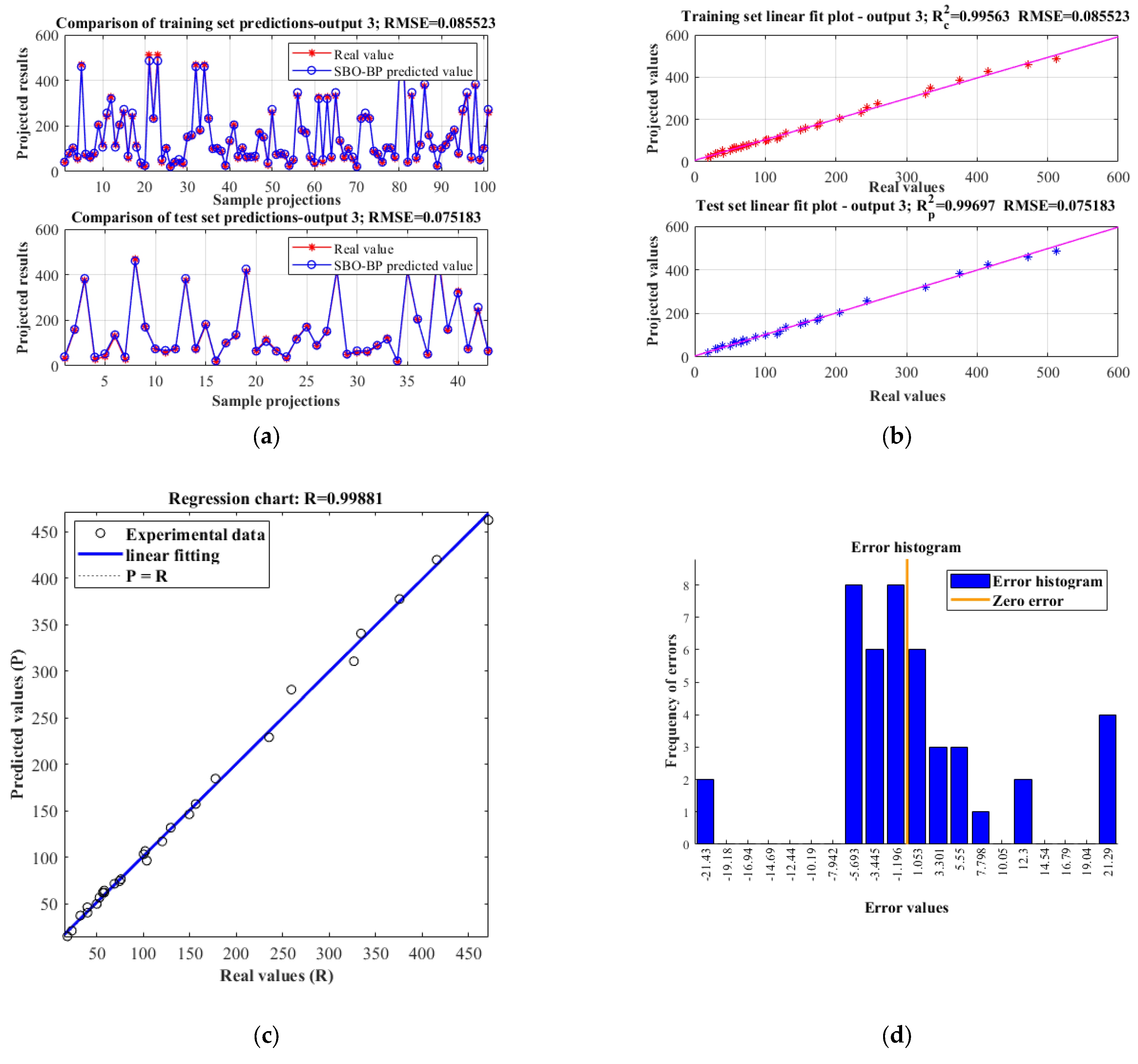
Third, for the task of predicting the rate of change of speed V_r at the end of the piston, the SBO–BP neural network model exhibits good modeling performance, as shown in Figure 18. The prediction results are highly consistent with the AMESim simulation values, with RMSEs of 0.085523 and 0.075183 for the training and test sets, respectively, and a correlation coefficient of 0.99881. In the linear fitting plot, the coefficients of determination of the training and test sets are 0.99563 and 0.99697, respectively, and the fitting curves are almost coincident with the ideal line, indicating that the model fitting accuracy is high. The error histogram shows that the errors are mainly concentrated near zero, with a more symmetrical distribution and less extreme errors, indicating that the model has strong stability and generalization ability, and is able to effectively predict the nonlinear characteristics of the rate of change of the speed at the end of the piston.

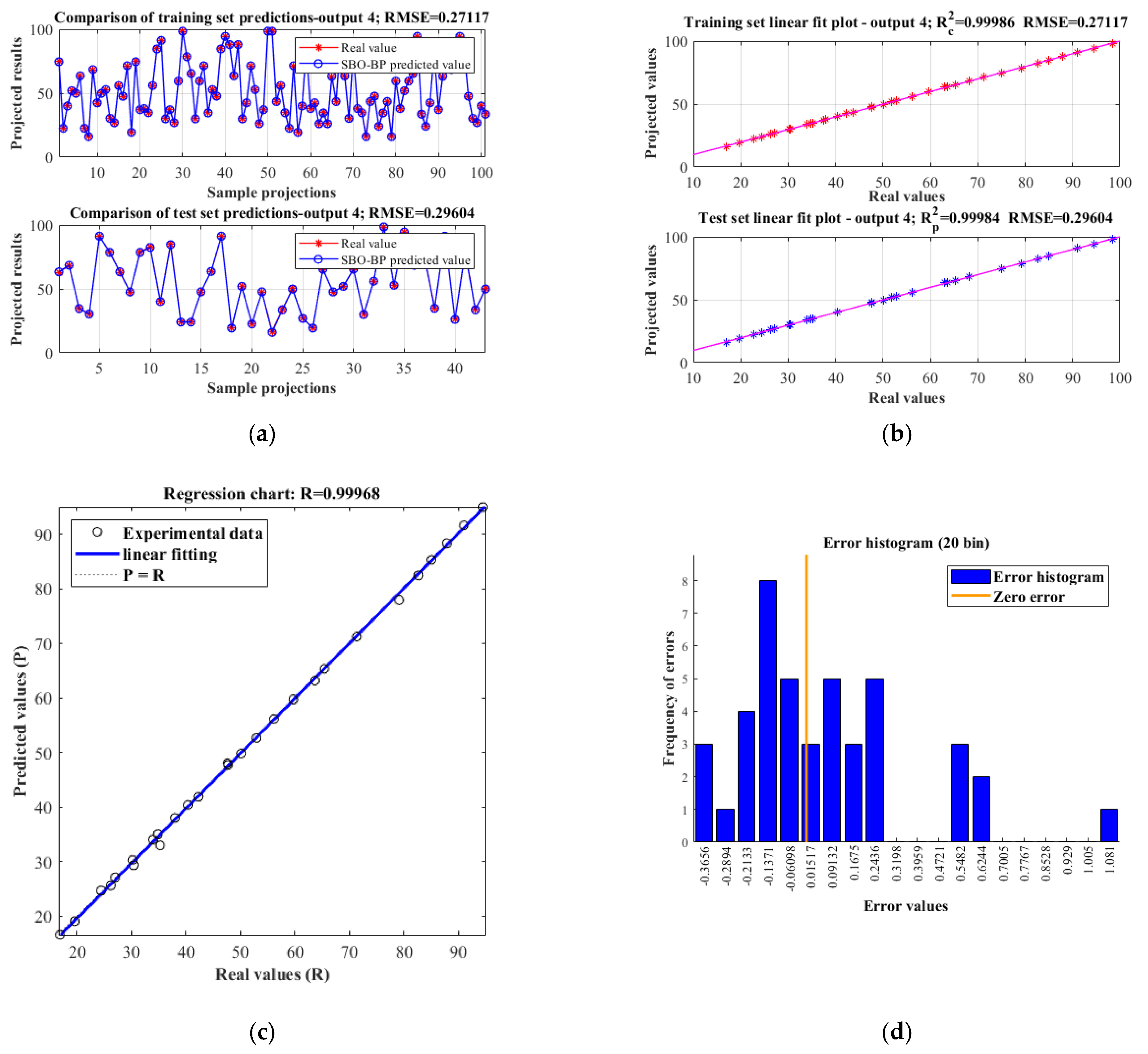
Finally, for the task of predicting the hydraulic oil reflux speed V_h, the SBO–BP neural network model exhibits excellent modeling performance, as shown in Figure 19. The RMSEs of the training and test sets are 0.27117 and 0.29604, respectively, and the prediction results are more consistent with the AMESim simulation values. The correlation coefficient in the regression plot reaches 0.99968, and the coefficient of determination in the linear fitting plot is 0.99986 and 0.99984 for the training and test sets, respectively, which indicates that the model’s fitting accuracy is high. The error histograms show that the errors are mainly concentrated around zero with a symmetrical distribution and few extreme errors, reflecting the good stability and generalization ability of the model over most samples, which is suitable for the accuracy modeling needs of hydraulic systems.

In order to further validate the accuracy of the SBO–BP prediction model, this thesis introduces four typical regression prediction performance evaluation metrics: the mean absolute percentage error (MAPE), the R-Square (R²), the mean absolute error (MAE), and the mean square error (MSE), and conducts comparative analyses among five improved BP neural network models. The above metrics comprehensively evaluate the model performance from multiple dimensions, such as error magnitude, relative accuracy and goodness-of-fit, aiming to reveal the differences in prediction accuracy and generalization ability among the models in a more systematic way.

(1)

Mean Absolute Percentage Error (MAPE)

MAPE is used to measure the average relative error of the predicted value relative to the actual value, reflecting the relative error level of the model at different magnitudes, calculated as Equation (24).

$$\mathrm{MAPE}={\displaystyle \frac{100\%}{n}}{\displaystyle \sum _{i=1}^n\left|\frac{{\stackrel{⌢}{y}}_i-y_i}{y_i}\right|}$$

(24)

where n denotes the total number of samples, y_i denotes the true value of the i-th sample and ${\overline{y}}_i$ denotes the predicted value of the i-th sample.

(2)

R-Square (R²)

R² is used to reflect the degree of fitting between the predicted value and the real value. The value domain is [0, 1], the closer to 1, the better the model fitting. The calculation formula is shown in Equation (25).

$${\mathrm{R}}^2=1-{\displaystyle \frac{{\displaystyle \sum _i{\left({\stackrel{⌢}{y}}_i-y_i\right)}^2}}{{\displaystyle \sum _i{\left({\overline{y}}_i-y_i\right)}^2}}}$$

(25)

where ${\overline{y}}_i$ is the average of the true values.

(3)

Mean Absolute Error (MAE)

MAE is used to measure the average absolute value of the difference between the predicted value and the true value with good interpretability and is calculated as Equation (26).

$$\mathrm{MAE}={\displaystyle \frac{1}{n}}{\displaystyle \sum _{i=1}^n\left|{\stackrel{⌢}{y}}_i-y_i\right|}$$

(26)

(4)

Mean Square Error (MSE)

MSE is used to measure the mean of the squared prediction errors, which is more sensitive to larger errors and is calculated as Equation (27).

$$\mathrm{MSE}={\displaystyle \frac{1}{m}}{{\displaystyle \sum _{i=1}^m\left(y_i-{\stackrel{⌢}{y}}_i\right)}}^2$$

(27)

From the analysis of the results in

Table 4. Comparison of the error of SBO–BP neural network prediction model results.

Predictive Modeling	Core Indicators	Data Set	Objective Function
			End Piston Speed Ve	Buffer Time T	Rate of Change of Speed at End of Piston Vr	Hydraulic Oil Return Speed Vh
NRBO–BP	MAPE (%)	Training set	2.1322 × 100	0.6600 × 100	4.8731 × 100	0.7637 × 100
		Test set	1.9137 × 100	0.6319 × 100	4.5722 × 100	0.7066 × 100
	R2	Training set	0.9985 × 100	0.9991 × 100	0.9990 × 100	0.9988 × 100
		Test set	0.9989 × 100	0.9990 × 100	0.9993 × 100	0.9988 × 100
	MAE(%)	Training set	5.6846 × 101	0.4565 × 100	4.4863 × 102	2.5378 × 101
		Test set	5.4486 × 101	0.4307 × 100	4.4369 × 102	2.5821 × 101
	MSE(%)	Training set	5.2307 × 101	4.4847 × 10−3	4.0755 × 103	1.1094 × 101
		Test set	4.5974 × 101	4.5153 × 10−3	3.7924 × 103	1.1614 × 101
GOOSE–BP	MAPE (%)	Training set	0.3904 × 100	0.7715 × 100	5.3288 × 100	0.9216 × 100
		Test set	0.5791 × 100	0.8731 × 100	7.7286 × 100	1.3876 × 100
	R2	Training set	0.9989 × 100	0.9987 × 100	0.9971 × 100	0.9985 × 100
		Test set	0.9989 × 100	0.9982 × 100	0.9968 × 100	0.9984 × 100
	MAE(%)	Training set	1.2714 × 101	0.5109 × 100	5.6076 × 102	3.7427 × 101
		Test set	1.6846 × 101	0.6691 × 100	5.3663 × 102	3.9838 × 101
	MSE(%)	Training set	8.0188 × 100	5.8049 × 10−3	5.3926 × 103	2.3809 × 101
		Test set	1.2404 × 101	9.5385 × 10−3	4.6334 × 103	3.2594 × 101
CPO–BP	MAPE (%)	Training set	0.6018 × 100	0.8972 × 100	4.4775 × 100	0.6019 × 100
		Test set	0.6002 × 100	0.8157 × 100	5.5056 × 100	0.5998 × 100
	R2	Training set	0.9997 × 100	0.9988 × 100	0.9970 × 100	0.9987 × 100
		Test set	0.9988 × 100	0.9987 × 100	0.9981 × 100	0.9988 × 100
	MAE(%)	Training set	2.3667 × 101	0.6002 × 100	5.3117 × 102	2.8407 × 101
		Test set	2.0061 × 101	0.5566 × 100	3.9755 × 102	2.4063 × 101
	MSE(%)	Training set	1.0063 × 101	6.1925 × 10−3	5.2238 × 103	1.4484 × 101
		Test set	6.2354 × 100	5.3684 × 10−3	3.1080 × 103	8.9616 × 100
SAO–BP	MAPE (%)	Training set	0.4573 × 100	1.0762 × 100	4.5263 × 100	1.3435 × 100
		Test set	0.5003 × 100	1.4696 × 100	5.8078 × 100	1.3938 × 100
	R2	Training set	0.9989 × 100	0.9974 × 100	0.9979 × 100	0.9988 × 100
		Test set	0.9989 × 100	0.9968 × 100	0.9963 × 100	0.9988 × 100
	MAE(%)	Training set	1.5842 × 101	0.7485 × 100	4.4903 × 102	2.3668 × 101
		Test set	1.6579 × 101	0.9443 × 100	5.7178 × 102	2.7573 × 101
	MSE(%)	Training set	3.8903 × 100	0.0124 × 100	3.7426 × 103	4.9737 × 101
		Test set	4.3544 × 100	0.0151 × 100	6.2295 × 103	4.4861 × 101
BMO–BP	MAPE (%)	Training set	0.4923 × 100	0.8395 × 100	4.8988 × 100	0.6458 × 100
		Test set	0.5045 × 100	0.9369 × 100	8.8641 × 100	0.6823 × 100
	R2	Training set	0.9989 × 100	0.9976 × 100	0.9972 × 100	0.9988 × 100
		Test set	0.9989 × 100	0.9963 × 100	0.9954 × 100	0.9989 × 100
	MAE(%)	Training set	1.5342 × 101	0.5639 × 100	4.5913 × 102	2.5801 × 101
		Test set	1.8465 × 101	0.7595 × 100	6.9504 × 102	2.4719 × 101
	MSE(%)	Training set	3.7272 × 100	9.9777 × 10−3	4.4766 × 103	1.0315 × 101
		Test set	5.3076 × 100	0.0217 × 100	9.2907 × 103	8.4288 × 100
SBO–BP	MAPE (%)	Training set	0.5003 × 100	0.5808 × 100	4.1542 × 100	0.5914 × 100
		Test set	0.4397 × 100	0.6765 × 100	5.5685 × 100	0.7324 × 100
	R2	Training set	0.9998 × 100	0.9995 × 100	0.9989 × 100	0.9991 × 100
		Test set	0.9998 × 100	0.9993 × 100	0.9988 × 100	0.9997 × 100
	MAE(%)	Training set	1.4637 × 101	0.3817 × 100	2.8562 × 102	1.3435 × 100
		Test set	1.9661 × 101	0.4661 × 100	2.9687 × 102	1.3938 × 100
	MSE(%)	Training set	2.7541 × 100	2.7318 × 10−3	1.6061 × 103	9.1869 × 100
		Test set	4.2783 × 100	3.6399 × 10−3	1.4493 × 103	1.0317 × 101

, it can be seen that the SBO–BP model performs well in a number of key performance evaluation indexes and is significantly better than the other compared models, including NRBO–BP, GOOSE–BP, CPO–BP, SAO–BP and BMO–BP. Specifically, in terms of R², the SBO–BP model maintains a high level above 0.999 on both the training and test sets, which is better than some of the comparison models, fully demonstrating the good generalization performance of the model. For example, in the prediction of “End-piston speed V_e” and “End-piston speed change rate V_r”, the R² values of the test set of the SBO–BP model reach above 0.9998, which is at the leading level. In terms of the error category, SBO–BP also shows lower prediction bias. In the prediction of “Buffer time T”, the mean absolute percentage error (MAPE) of the test set is 0.5808%, and the mean absolute error (MAE) is 0.3817%, which are significantly better than the other models, showing higher prediction accuracy. Meanwhile, in the prediction task of “hydraulic oil reflux speed V_h”, the mean square error (MSE) of SBO–BP is 1.0317 × 10¹, which is lower than that of some comparative algorithms, further verifying its stability and robustness. In summary, the SBO–BP model performs well in various evaluation indexes, combining high accuracy, strong fitting ability and good generalization performance.

5. Optimization of EHA Buffer Structure Based on NSGA-II

5.1. Objective Function and Constraint Setting

In order to improve the performance of the small-cavity buffer structure of a certain type of EHA hydraulic cylinder, this thesis carried out a multi-objective optimization design based on the prediction model constructed in Part 4 coupled with NSGA-II. The optimization objective aims to simultaneously minimize the following four key performance indicators: buffer time T, end-of-piston speed V_e, end-of-piston speed change rate V_r, and hydraulic oil return speed V_h, in order to achieve fast response, stable control and reasonable energy return in the buffer process. The set multi-objective optimization function is shown as Equation (28), and the value ranges and constraints of the optimization variables are detailed in Equation (29).

$$\min \left\{\begin{array}{c}{F}_1\left(G,D,\theta ,L_1\right)=V_e\\ F_2\left(G,D,\theta ,L_1\right)=T\\ F_3\left(G,D,\theta ,L_1\right)=V_r\\ F_4\left(G,D,\theta ,L_1\right)=V_h\end{array}\right.$$

(28)

$$s.t.\left\{\begin{array}{cc}0.05\le G\le 0.1& \left(\mathrm{mm}\right)\\ 0.5\le D\le 1& \left(\mathrm{mm}\right)\\ {0.5}^{\circ }\le \theta \le 3^{\circ }& \left(\mathrm{Angle}\right)\\ 35\le L_1\le 43& \left(\mathrm{mm}\right)\end{array}\right.$$

(29)

5.2. Multi-Objective Optimization Experiment

In the multi-objective optimization process, this thesis adopts the prediction model based on an SBO–BP neural network as the computational carrier of the objective function, which is used to evaluate the performance of the buffer structure under different combinations of parameters.

To evaluate the robustness and stability of the proposed NSGA-II-based multi-objective optimization framework, a sensitivity analysis was conducted on its key algorithmic parameters, namely the population size, crossover probability (P_c), and mutation probability (P_m). These parameters directly affect the convergence behavior and the diversity of Pareto-optimal solutions.

The sensitivity analysis was performed by systematically varying one parameter at a time while keeping the others constant. The baseline configuration was set as: population size = 100, P_c = 0.9, and P_m = 0.05. The results of the sensitivity test are shown in Table 5.

• Population Size: Increasing the population from 50 to 150 improved the solution quality and diversity. However, diminishing returns were observed beyond 100 individuals, indicating a trade-off between computational costs and marginal performance gains.
• Crossover Probability: A high crossover rate (0.8–0.9) yielded more consistent convergence. Lower values (<0.7) often led to premature convergence and limited exploration of the design space.
• Mutation Probability: Moderate mutation rates (0.05–0.2) helped maintain diversity. Excessively low mutation (<0.01) resulted in stagnation, while very high values (>0.25) introduced instability in convergence.

Table 5. Sensitivity Analysis of NSGA-II Parameters.

Parameter	Values Tested	Min Piston Velocity (m/s)	Cushioning Time T (s)	Observation
Population Size	50/100/150	0.0102/0.0061/0.0060	0.63/0.73/0.82	Best performance at 100–150
Crossover Rate (Pc)	0.6/0.8/0.9	0.0123/0.0064/0.0065	0.78/0.69/0.80	0.8–0.9 range is optimal
Mutation Rate (Pm)	0.01/0.05/0.2	0.0075/0.0070/0.0061	0.74/0.81/0.76	Moderate mutation yields stability

Table 5. Sensitivity Analysis of NSGA-II Parameters.

Parameter	Values Tested	Min Piston Velocity (m/s)	Cushioning Time T (s)	Observation
Population Size	50/100/150	0.0102/0.0061/0.0060	0.63/0.73/0.82	Best performance at 100–150
Crossover Rate (Pc)	0.6/0.8/0.9	0.0123/0.0064/0.0065	0.78/0.69/0.80	0.8–0.9 range is optimal
Mutation Rate (Pm)	0.01/0.05/0.2	0.0075/0.0070/0.0061	0.74/0.81/0.76	Moderate mutation yields stability

These results suggest that the NSGA-II algorithm is relatively robust within a reasonable parameter range. The chosen default configuration (population = 100, P_c = 0.85, P_m = 0.2) provides a good balance between convergence speed and solution diversity in the context of hydraulic buffer structural optimization.

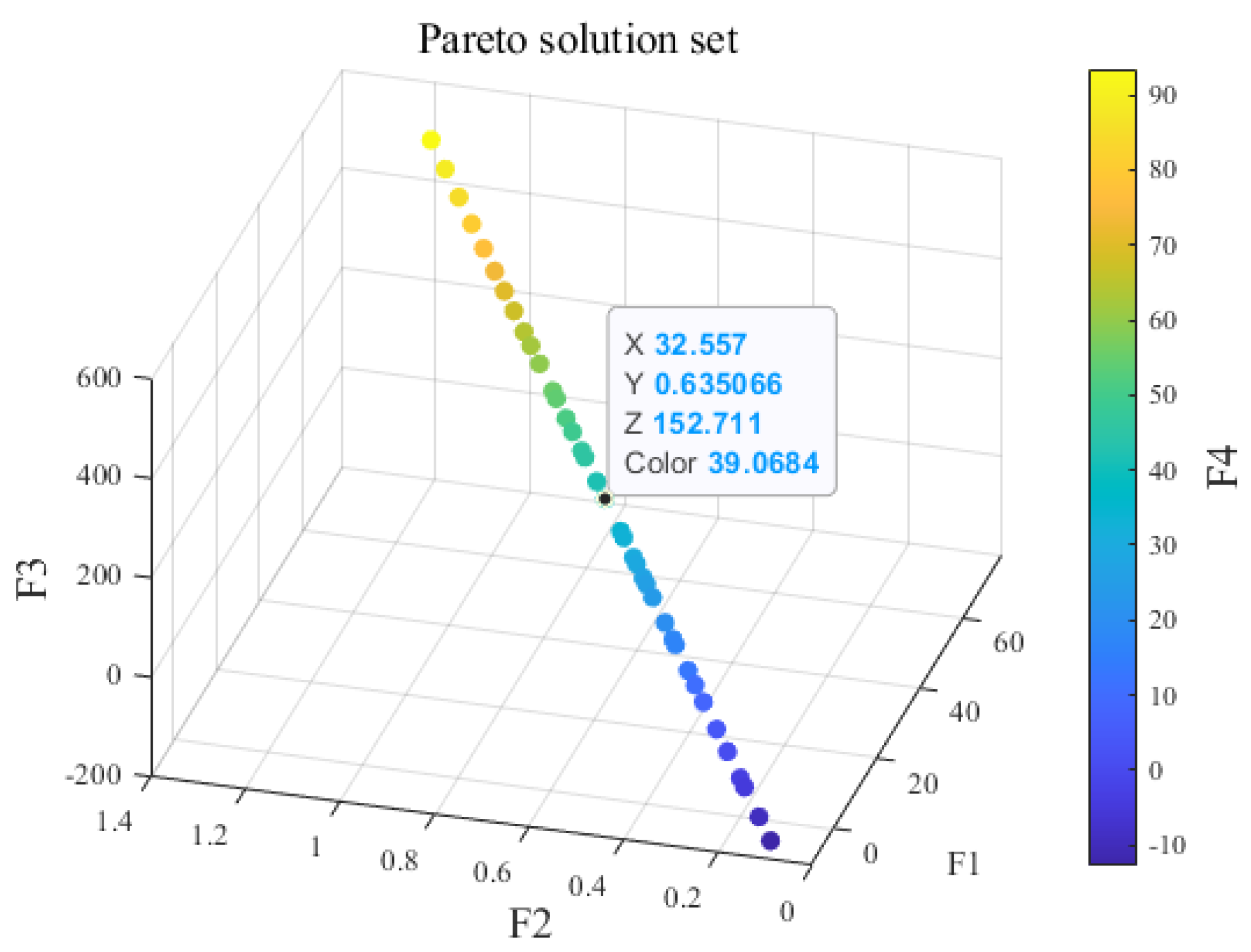
The Pareto-optimal solution set shown in Figure 20 is obtained by coupling the NSGA-II algorithm for solving. The results show that there are significant coupling relationships and mutual constraints between the optimization objective functions, and it is difficult to achieve the optimal value of each performance index in the same solution at the same time. Therefore, it is necessary to consider the practical factors such as process feasibility, manufacturing cost and engineering adaptability when selecting parameters, and select the optimal compromise solution from the Pareto front.

As shown in the markings of Figure 20, the selected compromise optimal parameter combinations are: fitting clearance G = 0.036 mm, fixed orifice diameter D = 0.95 mm, wedge face angle $\theta$ = 2.31°, and wedge face length L₁ = 38.76 mm. Under this parameter combination, the output performance indicators predicted based on the SBO–BP model are: end-piston speed V_e = 32.557 mm/s, cushioning time T = 0.635 s, change rate of end-piston speed V_r = 152.711 mm/s, and return speed of hydraulic oil V_h = 39.0684 mm/s.

This solution achieves a better balance among multiple performance objectives and reflects a good cushioning effect and system stability. The solution achieves a better balance between multiple performance objectives, reflects a good buffering effect and system stability, and has practical engineering application value.

In order to verify the effectiveness of the optimization strategy, we carried out a comparative simulation analysis of the buffer structure of the small cavity of the hydraulic cylinder before and after the optimization. The detailed experimental data are shown in

Table 6. Output Core Parameter Experiment Results.

Output Core Parameters	Pre-Optimization	Post-Optimization
Ve$(\mathrm{m}\cdot {\mathrm{s}}^{-1}$)	0.060	0.032
Vr$(\mathrm{m}\cdot {\mathrm{s}}^{-1}$)	0.244	0.153
Vh$(\mathrm{m}\cdot {\mathrm{s}}^{-1}$)	0.073	0.039
T (s)	0.5	0.6325

. Except for the key optimization parameters—fitting clearance G, fixed orifice diameter D, wedge face angle $\theta$ and wedge face length L₁—the rest of the structure and control parameters remain consistent.

The experimental results show that the optimized structure exhibits a significant improvement in the key performance indexes, in which the end-piston speed V_e is reduced from 0.060 m/s before optimization to 0.032 m/s after optimization, with a decrease of about 46.7%, the rate of change of end-piston speed V_r is reduced from 0.244 m/s before optimization to 0.153 m/s after optimization, with a decrease of about 37.3%, and the hydraulic oil return speed V_h is reduced from 0.073 m/s before optimization to 0.039 m/s after optimization, with a decrease of about 46.5%. The optimized cushioning structure of the EHA hydraulic cylinder significantly increases the deceleration capacity of the cushioning end, which effectively suppresses the possible impact of the piston at the end of its stroke. Although the buffer time increases slightly from 0.5 s to 0.6325 s, the change does not have a significant impact on the overall efficiency of the equipment, and it still meets the response speed requirements of engineering operation. In summary, the optimized small-cavity buffer structure of the EHA hydraulic cylinder significantly reduces the end-piston speed and improves the dynamic performance of the buffer stage on the basis of maintaining the working efficiency of the system, which helps to improve the smoothness and safety of the end operation of the EHA hydraulic cylinder, and it has a good value of engineering promotion.

6. Discussion

This study aimed to address the end impact problem of a small cavity buffer in a certain type of EHA hydraulic cylinder. Through mechanism analysis, machine–hydraulic co-simulation modeling, and a combination of enhanced neural network prediction and multi-objective optimization, several critical insights were gained regarding the influence of buffer structural parameters and the effectiveness of the proposed optimization strategy.

First, the simulation and sensitivity analysis revealed that the fitting clearance (G) between the buffer sleeve and buffer hole and the diameter of the fixed damping orifice (D) are the most influential factors affecting the piston end velocity. In contrast, wedge face angle $\theta$ and wedge face length (L₁) showed comparatively minor impacts on the terminal deceleration effect. This indicates that during structural design, priority should be given to controlling the tolerances of the buffer fitting and the damping orifice size. The observed monotonic relationship—where increasing either G or D leads to increased piston end speed—is consistent with expected physical behavior, as larger gaps or orifices reduce flow resistance, thereby weakening the cushioning effect. This insight helps guide engineers to avoid over-sizing these parameters during buffer design.

Second, the SBO-enhanced BP neural network model demonstrated excellent predictive capability for key performance indicators including buffer time (T), end-piston velocity (V_e), velocity change rate (V_r), and hydraulic oil return velocity (V_h). The enhanced model showed improved accuracy and generalization compared to traditional BP networks, owing to the global search and adaptive behavior of the SBO algorithm. This predictive model not only accelerates the evaluation process within optimization loops but also provides an effective approximation of the objective function for use in multi-objective evolutionary algorithms. The successful integration of machine learning and domain-specific simulation offers a promising pathway for data-driven modeling in complex hydraulic systems.

Third, the NSGA-II-based multi-objective optimization led to a significant improvement in system performance. Specifically, the optimized buffer structure achieved a 46.7% reduction in piston end velocity while only marginally increasing the buffer time from 0.5 s to 0.6325 s. This result demonstrates a well-balanced trade-off between cushioning effectiveness and system efficiency. It also highlights the value of Pareto-based optimization in identifying design configurations that simultaneously satisfy multiple and often conflicting performance criteria. Importantly, the optimized parameters remain within practical manufacturing tolerances, indicating the feasibility of applying these results in real-world EHA systems.

Finally, the proposed SBO–BP + NSGA-II methodology is inherently scalable to different EHA configurations. Design parameters such as piston diameter, chamber area and stroke length can be reparametrized to accommodate various actuator sizes and application-specific demands. Practitioners are advised to generate a modest number of simulation data samples for each new actuator design, followed by retraining the SBO–BP model and rerunning of the NSGA-II optimization under updated constraints. This workflow enables efficient customization of buffer structures across a wide range of industrial and aerospace scenarios.

Overall, the findings of this study not only demonstrate the effectiveness of the proposed optimization framework in solving a specific buffering problem, but also establish its practical feasibility, adaptability and cost-effectiveness for broader use in real-world EHA systems.

7. Conclusions

This study investigates the mitigation of end-impact problems in the small cavity of a specific type of electro-hydrostatic actuator (EHA) hydraulic cylinder through structural optimization of the buffer chamber. By analyzing the internal buffering mechanism, four critical structural parameters—the fitting clearance G between the buffer sleeve and buffer hole, the diameter of the fixed orifice D, the wedge surface angle $\theta$, and the wedge surface length L₁—were selected for detailed evaluation. An AMESim-based machine–hydraulic co-simulation model was established to replicate the dynamic response of the small-chamber buffer process under various design conditions.

To enhance optimization efficiency and predictive accuracy, a hybrid SBO–BP neural network was constructed to model the piston end velocity and buffer time with high fidelity, achieving a mean absolute percentage error (MAPE) below 1% for both objectives. The predictive model was further embedded into a multi-objective NSGA-II optimization framework. The results revealed that the fitting clearance and orifice diameter significantly influence piston end velocity, while the wedge surface parameters have relatively minor effects. The final optimized design achieved a 46.7% reduction in piston end velocity, effectively solving the end-impact problem without compromising operational efficiency, as validated through full-system experimental testing.

Beyond this specific application, the proposed method—combining physics-based modeling, intelligent prediction and multi-objective optimization—can be generalized to buffer design in other EHA systems, hydraulic actuators in aerospace and robotics, and similar fluid-structure interaction systems where impact control and structural trade-offs are critical. However, this study has several limitations. First, the predictive model was trained on simulated data, and although validated by experiments, further generalization to broader operating conditions or actuator types may require domain adaptation. Second, temperature effects, component wear and long-term degradation were not considered in the simulation or optimization, which could affect real-world robustness. Future work will focus on incorporating thermal–mechanical coupling effects, expanding the dataset with real operational data, and exploring real-time onboard deployment of the proposed optimization method.

References

1. Lv, J.; Huang, B.; Qiang, L. Continuous prediction of knee joint angle in lower limbs based on sEMG: A method combining an improved ZOA optimizer and attention-enhanced GRU. J. King Saud Univ. Comput. Inf. Sci. 2025, 37, 149. [Google Scholar] [CrossRef]
2. Du, S.; Zhou, J.; Hong, J.; Zhao, H.; Ma, S. Application and progress of high-efficiency electro-hydrostatic actuator technology with energy recovery: A comprehensive review. Energy Convers. Manag. 2024, 321, 119041. [Google Scholar] [CrossRef]
3. Jiao, Z.; Li, Z.; Shang, Y.; Wu, S.; Song, Z.; Pan, Q. Active load sensitive electro-hydrostatic actuator on more electric aircraft: Concept, design, and control. IEEE Trans. Ind. Electron. 2021, 69, 5030–5040. [Google Scholar] [CrossRef]
4. Adamu, S.; Alhussian, H.; Abdulkadir, S.J.; Alwadin, A.; Khairy, S.O. Adaptive hybrid hyperparameter optimization with MRFO and Lévy flight for accurate melanoma classification. J. King Saud Univ. Comput. Inf. Sci. 2025, 37, 64. [Google Scholar] [CrossRef]
5. Chao, Q.; Zhang, J.; Xu, B.; Huang, H.; Pan, M. A review of high-speed electro-hydrostatic actuator pumps in aerospace applications: Challenges and solutions. J. Mech. Des. 2019, 141, 050801. [Google Scholar] [CrossRef]
6. Fan, J.; Qu, L. A multi-strategy improved sparrow search algorithm for mobile robots path planning. Meas. Sci. Technol. 2024, 35, 106207. [Google Scholar] [CrossRef]
7. Lazutkin, S.L.; Lazutkina, N.A. Perspective construction of hydraulic impact device. Procedia Eng. 2015, 129, 403–407. [Google Scholar] [CrossRef][Green Version]
8. Ding, S.; Li, G.; Shi, Y.; Ma, J.; Gao, M. Failure analysis of a loader hydraulic cylinder and its end cap structure improvement. Eng. Fail. Anal. 2023, 153, 107597. [Google Scholar] [CrossRef]
9. Gad, O. Dynamic modeling and simulation of impact in hydraulic cylinders. Proc. Inst. Mech. Eng. Part C J. Mech. Eng. Sci. 2021, 235, 5216–5233. [Google Scholar] [CrossRef]
10. Zhao, X.; Zhu, X.; Liu, J.; Hu, Y.; Gao, T.; Liu, Z. Model-assisted multi-source fusion hypergraph convolutional neural networks for intelligent few-shot fault diagnosis to electro-hydrostatic actuator. Inf. Fusion 2024, 104, 102186. [Google Scholar] [CrossRef]
11. Liu, J.; Yao, J.; Deng, W. Nonlinear robust adaptive control of Electro-hydrostatic actuators with continuous friction compensation. Int. J. Control Autom. Syst. 2024, 22, 1225–1237. [Google Scholar] [CrossRef]
12. Jiang, H.; Ling, Z.; Zhou, F.; Yang, H. Adaptive Dead Zone Compensation Control Method for Electro-Hydrostatic Actuators Under Low-Speed Conditions. Chin. J. Mech. Eng. 2024, 37, 168. [Google Scholar] [CrossRef]
13. Zhang, T.; Yan, G.; Liu, X.; Yao, C.; Ai, C. Nonlinear flow modeling of electro hydrostatic pump unit based on Gauss Newton iterative method for high performance control. Sci. Rep. 2024, 14, 21750. [Google Scholar] [CrossRef] [PubMed]
14. Ma, Z.; Liao, H.; Gao, J.; Nie, S.; Geng, Y. Physics-informed machine learning for degradation modeling of an electro-hydrostatic actuator system. Reliab. Eng. Syst. Saf. 2023, 229, 108898. [Google Scholar] [CrossRef]
15. Zhu, T.; Xie, H.; Yang, H. Design and tracking control of an electro-hydrostatic actuator for a disc cutter replacement manipulator. Autom. Constr. 2022, 142, 104480. [Google Scholar] [CrossRef]
16. Liu, J.; Hu, Y.; Zhu, X.; Zhao, X.; Yao, J. Intelligent fault diagnosis for electro-hydrostatic actuator based on multisource information convolutional residual network. Meas. Sci. Technol. 2024, 35, 066114. [Google Scholar] [CrossRef]
17. Xing, X.; Luo, Y.; Han, B.; Qin, L.; Xiao, B. Hybrid Data-Driven and Multisequence Feature Fusion Fault Diagnosis Method for Electro-Hydrostatic Actuators of Transport Airplane. IEEE Trans. Ind. Inform. 2025, 21, 3306. [Google Scholar] [CrossRef]
18. Rodriguez-Aguilar, R.; Marmolejo-Saucedo, J.A.; Köse, U. Development of a digital twin driven by a deep learning model for fault diagnosis of electro-hydrostatic actuators. Mathematics 2024, 12, 3124. [Google Scholar] [CrossRef]
19. Kumar, G.; Mandal, N.P. Position control performance analysis of linear actuator in swashplate-controlled electro hydrostatic actuation system. Eng. Res. Express 2023, 5, 045087. [Google Scholar] [CrossRef]
20. Wang, J.; Chen, Y.; Lu, C.; Heidari, A.A.; Wu, Z.; Chen, H. The Status-based Optimization: Algorithm and comprehensive performance analysis. Neurocomputing 2025, 647, 130603. [Google Scholar] [CrossRef]
21. Deb, K.; Pratap, A.; Agarwal, S.; Meyarivan, T.A.M.T. A fast and elitist multiobjective genetic algorithm: NSGA-II. IEEE Trans. Evol. Comput. 2002, 6, 182–197. [Google Scholar] [CrossRef]
22. Huang, X.; Zhixiong, L.; Xuefeng, B.; Honglei, P. Research on tractor tillage depth control based on AMESim-Matlab joint simulation. J. Chin. Agric. Mech. 2024, 45, 9–15. [Google Scholar] [CrossRef]
23. Jiang, J.; Xu, G.; Wang, H.; Yang, Z.; Chen, X. High-accuracy road surface condition detection through multi-sensor information fusion based on WOA-BP neural network. Sens. Actuators A Phys. 2024, 378, 115829. [Google Scholar] [CrossRef]
24. Ahmadi, S.A. Human behavior-based optimization: A novel metaheuristic approach to solve complex optimization problems. Neural Comput. Appl. 2017, 28, 233–244. [Google Scholar] [CrossRef]
25. Lian, J.; Zhu, T.; Ma, L.; Wu, X.; Hui, G. The educational competition optimizer. Int. J. Syst. Sci. 2024, 55, 3185–3222. [Google Scholar] [CrossRef]
26. Khishe, M.; Jangir, P.; Arpita; Agrawal, S.P.; Pandya, S.B.; Parmar, A.; Abualigah, L. Innovative Diversity Metrics in Hierarchical Population-Based Differential Evolution for PEM Fuel Cell Parameter Optimization. Eng. Rep. 2025, 7, e13065. [Google Scholar] [CrossRef]
27. Ibrahim, N.; Hassan, F.H.; Syed-Mohamad, S.M.; Mohemad, R.; Mohd Noor, A.S. Comparative Analysis of Rank and Roulette Wheel Selection Strategies in Genetic Algorithms for Spatial Layout Optimization. Int. J. Adv. Comput. Sci. Appl. 2025, 16, 574. [Google Scholar] [CrossRef]
28. Moy, C.; Czenszak, J.; Li, J.M.; Marshall, B.; Holtzen, S. Roulette: A Language for Expressive, Exact, and Efficient Discrete Probabilistic Programming. Proc. ACM Program. Lang. 2025, 9, 2081–2105. [Google Scholar] [CrossRef]
29. Wang, X.; Snášel, V.; Mirjalili, S.; Pan, J.S. MAAPO: An innovative membrane algorithm based on artificial protozoa optimizer for multilevel threshold image segmentation. Artif. Intell. Rev. 2025, 58, 324. [Google Scholar] [CrossRef]
30. Sowmya, R.; Premkumar, M.; Jangir, P. Newton-Raphson-based optimizer: A new population-based metaheuristic algorithm for continuous optimization problems. Eng. Appl. Artif. Intell. 2024, 128, 107532. [Google Scholar] [CrossRef]
31. Hamad, R.K.; Rashid, T.A. GOOSE algorithm: A powerful optimization tool for real-world engineering challenges and beyond. Evol. Syst. 2024, 15, 1249–1274. [Google Scholar] [CrossRef]
32. Guo, Z.; Liu, G.; Jiang, F. Chinese Pangolin Optimizer: A novel bio-inspired metaheuristic for solving optimization problems. J. Supercomput. 2025, 81, 517. [Google Scholar] [CrossRef]
33. Deng, L.; Liu, S. Snow ablation optimizer: A novel metaheuristic technique for numerical optimization and engineering design. Expert Syst. Appl. 2023, 225, 120069. [Google Scholar] [CrossRef]
34. Rodan, A.; Al-Tamimi, A.K.; Al-Alnemer, L.; Mirjalili, S.; Tiňo, P. Enzyme action optimizer: A novel bio-inspired optimization algorithm. J. Supercomput. 2025, 81, 686. [Google Scholar] [CrossRef]
Figure 1. Electro-Hydrostatic Actuator system structure.
Mathematics 13 02960 g001
Figure 2. EHA hydraulic cylinder small cavity buffer structure schematic diagram.
Mathematics 13 02960 g002
Figure 3. EHA Hydraulic Cylinder Small Cavity Cushion Simulation Model.
Mathematics 13 02960 g003
Figure 4. Displacement-buffer chamber pressure variation curves for different fitting clearances G.
Mathematics 13 02960 g004
Figure 5. Displacement-piston speed variation curves for different fitting clearances G.
Mathematics 13 02960 g005
Figure 6. Displacement-buffer chamber pressure variation curves for different D.
Mathematics 13 02960 g006
Figure 7. Displacement-piston speed variation curves for different D.
Mathematics 13 02960 g007
Figure 8. Displacement-buffer chamber pressure variation curves for different θ .
Mathematics 13 02960 g008
Figure 9. Displacement-piston speed variation curves for different θ .
Mathematics 13 02960 g009
Figure 10. Displacement-buffer chamber pressure variation curves for different L1.
Mathematics 13 02960 g010
Figure 11. Displacement-piston speed variation curves for different L1.
Mathematics 13 02960 g011
Figure 12. Elite Engagement phase of SBO.
Mathematics 13 02960 g012
Figure 13. Resource acquisition phase of SBO.
Mathematics 13 02960 g013
Figure 14. Flowchart for selecting the optimal number of hidden layers.
Mathematics 13 02960 g014
Figure 15. Comparison of algorithm convergence plots.
Mathematics 13 02960 g015
Figure 16. Experimental chart of the end-piston velocity Ve prediction model. (a) Forecast comparison chart. (b) Linear fitting chart. (c) Regression chart. (d) Error histogram.
Mathematics 13 02960 g016
Figure 17. Experimental chart of the buffer time T prediction model. (a) Forecast comparison chart. (b) Linear fitting chart. (c) Regression chart. (d) Error histogram.
Mathematics 13 02960 g017
Figure 18. Experimental chart of the predictive model for the rate of change of speed Vr at the end of the piston. (a) Forecast comparison chart. (b) Linear fitting chart. (c) Regression chart. (d) Error histogram.
Mathematics 13 02960 g018
Figure 19. Experimental chart of hydraulic fluid return speed Vh prediction model. (a) Forecast comparison chart. (b) Linear fitting chart. (c) Regression chart. (d) Error histogram.
Mathematics 13 02960 g019
Figure 20. Multi-objective Optimization of Pareto Frontier Solution Sets.
Mathematics 13 02960 g020