Article

A Multi-View Fusion Data-Augmented Method for Predicting BODIPY Dye Spectra

The College of Information, Mechanical and Electrical Engineering, Shanghai Normal University, Shanghai 201418, China
*
Author to whom correspondence should be addressed.
Mathematics 2025, 13(18), 2947; https://doi.org/10.3390/math13182947
Submission received: 13 August 2025 / Revised: 6 September 2025 / Accepted: 10 September 2025 / Published: 11 September 2025

Abstract

Fluorescent molecules, particularly BODIPY dyes, have found wide applications in fields such as bioimaging and optoelectronics due to their excellent photostability and tunable spectral properties. In recent years, artificial intelligence methods have enabled more efficient screening of molecules, allowing the required molecules to be quickly obtained. However, existing methods remain inadequate to meet research needs, primarily due to incomplete molecular feature extraction and the scarcity of data under small-sample conditions. In response to the aforementioned challenges, this paper introduces a spectral prediction method that integrates multi-view feature fusion and data augmentation strategies. The proposed method consists of three modules. The molecular feature engineering module constructs a multi-view molecular fusion feature that includes molecular fingerprints, molecular descriptors, and molecular energy gaps, which can more comprehensively obtain molecular feature information. The data augmentation module introduces strategies such as SMILES randomization, molecular fingerprint bit-level perturbation, and Gaussian noise injection to enhance the performance of the model in small sample environments. The spectral prediction module captures the complex mapping relationship between molecular structure and spectrum. It is demonstrated that the proposed method provides considerable advantages in the virtual screening of organic fluorescent molecules and offers valuable support for the development of novel BODIPY derivatives based on data-driven strategies.

1. Introduction

Fluorescent materials have found extensive applications across a wide range of advanced research domains, such as bioimaging, sensors, lasers, optoelectronic devices, and photonics, due to their excellent optical stability, tunable emission wavelengths, and high sensitivity to environmental stimuli [1,2,3]. In particular, for biomedical applications such as in vivo imaging and cellular labeling, fluorescent molecules with high selectivity, a high signal-to-noise ratio, and exceptional photostability serve as key tools for achieving high-resolution detection and dynamic monitoring [4]. However, conventional fluorescent dyes still face numerous limitations in practical applications. For instance, they often suffer from poor water solubility, which makes it challenging to stably disperse in physiological conditions. Moreover, they tend to undergo aggregation-caused quenching (ACQ) at high concentrations or in aggregated states, leading to a significant decrease in fluorescence intensity and signal stability [5,6]. In addition, these dyes typically exhibit low structural rigidity, limited functionalization capability, and a lack of reactive sites, which severely hampers their multifunctional development in complex biological systems.
Fortunately, fluorescent dyes developed based on the boron-dipyrromethene (BODIPY) core offer an ideal solution to overcome the challenges above. BODIPY molecules possess a unique planar rigid structure, high molar extinction coefficients, high fluorescence quantum yields, excellent chemical stability, and are amenable to facile functional group modifications [7]. These features increase its stability in extreme conditions and allow for a high degree of adjustability. As a result, BODIPY dyes have emerged as a focal point of research in the field of fluorescent molecules in recent years, finding broad applications in the development of biological probes, molecular imaging, drug delivery, and photodynamic therapy [8,9].
In the design and development of modern molecular optical functional materials, constructing BODIPY molecules with specific absorption and emission spectral properties has become a research focus. BODIPY-based fluorescent probes with different emission wavelengths can meet various application needs based on their spectral characteristics. For instance, BODIPY dyes emitting in the green (500–550 nm) and red (600–650 nm) regions are widely used for organelle imaging and fluorescent labeling [10]. In contrast, BODIPY derivatives that emit in the near-infrared (NIR) window (650–900 nm) offer advantages such as strong tissue penetration and minimal scattering and absorption interference, making them particularly suitable for deep-tissue imaging, real-time in vivo monitoring, and photodynamic therapy [11]. Moreover, due to their highly tunable structures, BODIPY dyes have been developed into various stimuli-responsive fluorescent probes for detecting target analytes such as metal ions, pH changes, and biological small molecules, thereby enabling highly sensitive and visual analysis of microenvironmental changes [12]. Therefore, selecting BODIPY molecules with appropriate absorption and emission wavelengths is crucial for the development of high-performance fluorescent probes.
However, traditional spectral characterization methods rely heavily on quantum chemical calculations such as density functional theory (DFT) [13], or require tedious molecular synthesis and experimental spectral validation [14]. These processes cannot be scaled up for high-throughput screening and are time-consuming and labor-intensive, with high cost risks under current demand conditions. Therefore, developing an efficient and accurate method for predicting spectral properties that can rapidly estimate the optical characteristics of molecules during the design stage has become one of the major challenges in enhancing the screening efficiency of fluorescent materials.
With the continuous evolution of machine learning (ML) and deep learning (DL) technologies, data-driven molecular design methods have emerged as a vital research direction for accelerating the discovery of functional molecules and the prediction of their spectral properties [15,16,17]. Compared with traditional methods that rely on quantum chemical calculations or experimental synthesis and validation, machine learning models are capable of capturing intricate nonlinear patterns between molecular structures and their optical, electronic, or pharmacological properties by modeling existing data, thereby enabling rapid property prediction and structure optimization. Numerous researchers have proposed a variety of predictive models based on different molecular representations and neural network architectures, achieving impressive results. For instance, Maya et al. developed a convolutional neural network (CNN) model using SMILES sequences as input, which was successfully applied to compound toxicity classification tasks and demonstrated outstanding performance on the classical TOX21 dataset, highlighting the effectiveness of sequence-based molecular representations in deep modeling [18]. Yuyang Wang et al. constructed a molecular graph contrastive learning framework that incorporates several graph augmentation strategies. These strategies significantly improved the generalization ability and stability of molecular graph representation learning across multiple benchmark datasets [19]. These studies demonstrate that incorporating diverse model architectures and data augmentation mechanisms can substantially enhance the model’s ability to capture underlying structure–property relationships in complex molecules. At the same time, molecular fingerprints such as morgan and daylight fingerprints, along with descriptors including molecular weight, topological polar surface area, and the number of hydrogen bond donors, have also been widely utilized as traditional yet effective molecular representations in regression and classification tasks [20]. While fingerprints focus on encoding the topological structure of molecules, descriptors reflect their physicochemical properties; combining both offers a multi-view input for models. In modern molecular modeling tasks, numerous studies have incorporated these features into deep learning frameworks to enhance the accuracy and stability of molecular property predictions [21].
Although the field of molecular property prediction has made significant progress with the assistance of artificial intelligence technology, several pressing challenges remain. These issues primarily stem from two key aspects. First, most existing predictive models are limited in terms of feature representation. Many studies extract molecular features from a single view, relying solely on one type of encoding such as SMILES sequences, molecular graphs, or molecular fingerprints. Relying on a single modality typically limits the ability to fully characterize the diverse structural and physicochemical attributes of molecules, thereby reducing the model’s sensitivity to critical properties and constraining its ability to learn complex structure–property relationships [22]. For example, relying only on molecular graphs or fingerprints may neglect important physicochemical attributes, which can have a significant impact on spectral characteristics such as fluorescence wavelength or emission intensity.
Moreover, molecular property prediction tasks heavily depend on high-quality, well-annotated datasets, the acquisition of which is often costly and time-consuming. In practical research, generating a single molecular spectral profile or acquiring a biological activity label typically requires complex synthesis, characterization, or biological assays. For instance, the widely used TOX21 dataset, which cost millions of dollars to construct, still contains only about 8000 molecules and 12 toxicity labels [23]. For certain rarer or more specialized properties, publicly available datasets may include only a few hundred molecules. Yang et al. [24] compared the performance of traditional machine learning methods with deep learning approaches across molecular datasets of varying sizes. They reported that when the sample size ranges from a few hundred to around one thousand, complex representation learning models (such as graph neural networks and Transformers) often struggle to achieve stable convergence. In such cases, their performance is not necessarily superior to that of traditional methods like random forests or support vector machines, and in some instances, a significant degradation in results can even be observed. Under such low-data conditions, models struggle to learn effectively and are prone to overfitting, thereby limiting their generalizability in real-world applications.
Therefore, this paper proposes a prediction framework based on multi-view feature fusion and data augmentation strategy, aiming to construct comprehensive and information-rich molecular representations for accurately predicting the spectrum of BODIPY molecules. The model integrates molecular features from multiple views, including molecular fingerprints, physicochemical descriptors, and predicted energy gap values. A hybrid molecular descriptor that integrates both structural and electronic information is obtained by fusing these heterogeneous features. This enriched representation is then fed into a spectral prediction module for downstream regression tasks. Predictive performance and generalization ability are further enhanced by incorporating multiple data augmentation strategies during training, with each applied independently to the corresponding training fold. These strategies generate perturbed yet chemically valid molecular variants, thereby enlarging the training data distribution and mitigating overfitting risks. The proposed method makes three contributions in predicting molecular spectral properties:
  • A multi-view feature fusion strategy combining molecular fingerprints and descriptors was adopted to extract features from different views, and a pre-trained regression model was employed to obtain the molecular energy gap as an electronic structural feature, which was subsequently incorporated into the feature engineering module;
  • Data augmentation strategies are applied exclusively to the training set during model training, effectively expanding the dataset size and enhancing the model’s generalization capability;
  • The effectiveness of the proposed strategies was validated through experiments, providing feasible insights into the field of molecular property prediction.
The remainder of this paper is organized as follows: Section 2 outlines the molecular feature engineering module of the proposed method, including the construction of molecular fusion features and the data augmentation strategy. Section 3 introduces the experimental setup, presents experimental results, and conducts an ablation study to verify the effectiveness of the proposed strategy. Section 4 concludes and discusses potential directions for future research.

2. Methods

2.1. Problem Definition

In the field of molecular spectral property prediction, it remains a significant challenge to efficiently and accurately extract key features from molecular structures to predict their optical properties. On one hand, existing methods often rely on a single type of molecular representation, such as SMILES strings, molecular fingerprints, or graph structures. This limitation hinders their ability to comprehensively capture the complex structural and physicochemical attributes of molecules, thereby restricting the overall predictive performance. On the other hand, acquiring experimental data for fluorescent molecules is typically time-consuming and costly. This issue is particularly pronounced in specific dye families such as BODIPY, where the available training data is often limited, further constraining the performance and generalization ability of deep learning models. To address these challenges, there is an urgent need for a predictive framework capable of integrating multi-view molecular features while maintaining strong generalization capability. Such a framework should be able to handle high-dimensional structural information and operate effectively in low-data regimes. A regression framework is designed by integrating self-predicted energy gap features and multiple data augmentation strategies, aiming to accurately and efficiently predict the spectrum of BODIPY molecules.
The dataset for molecular spectrum prediction consists of input–output pairs, referred to as samples. The definition of a sample is given as follows:
Definition 1 
(Sample for Molecular Spectrum Prediction). A sample for molecular spectrum prediction is a tuple ( S , λ ) , where
  • S is the SMILES sequence of a BODIPY molecule;
  • λ is the corresponding spectral property, either the absorption peak wavelength ( λ a b s ) or the emission peak wavelength ( λ e m i ).
The training dataset for molecular spectral prediction consists of a large number of such samples. Using the proposed property prediction framework, a mapping function from input to output can be learned, which is referred to as the prediction model. This model enables the prediction of both absorption and emission wavelengths for a given molecule.
Definition 2 
(Molecular Spectrum Prediction Model). Let S i denote a BODIPY molecule, and  S = { ( S 1 , λ 1 ) , ( S 2 , λ 2 ) , . . . , ( S n , λ n ) } be the training dataset containing n samples. A molecular spectrum prediction model is a valuation function f : S i R + learned from S .
If the model has good predictive performance, the difference between f ( S i ) and the true value λ i should be minimized. The learned function f can then be used to predict the spectral properties of unseen molecules.

2.2. Framework of the Method

The overall framework for spectral prediction is illustrated in Figure 1. It establishes a mapping between the SMILES representation of BODIPY molecules and their corresponding spectral properties using deep neural networks, enabling efficient prediction of molecular spectra within a limited time. The framework consists of three integrated components. First, the molecular feature engineering module extracts multiple types of representations from each SMILES sequence, including molecular fingerprints, physicochemical descriptors, and energy-related features such as HOMO/LUMO levels and energy gaps predicted by a pretrained regression model. These features are combined into a unified high-dimensional vector that captures both structural and electronic information. To improve generalization, the data augmentation module introduces variability through three complementary strategies: generating SMILES variants to increase sequence diversity, applying bit-level perturbations to molecular fingerprints, and injecting Gaussian noise into numerical features to simulate experimental uncertainty. Finally, the spectral prediction module receives the enriched feature vectors and outputs predicted absorption or emission wavelengths. During the model training phase, the network weights are continuously optimized by minimizing the error loss function to achieve efficient and accurate prediction of molecular spectral properties.

2.3. Molecular Feature Engineering Module

2.3.1. Acquisition and Complementarity of Molecular Descriptors and Fingerprints

Both molecular fingerprints and descriptors are utilized to capture complementary aspects of BODIPY molecules, allowing for a more complete representation of their structural and physicochemical characteristics. Molecular fingerprints provide an abstract representation of molecules. For example, morgan fingerprints and daylight fingerprints encode the molecular topology into a binary vector, where each bit indicates whether a fragment or structure exists in the molecule. This method effectively captures structural subunits and connectivity patterns, making it well suited for representing molecular shapes and structural motifs [25]. In contrast, molecular descriptors express global physicochemical properties in the form of numerical variables, including molecular weight, numbers of hydrogen-bond donors and acceptors, among others. These properties reflect the electronic structure and chemical characteristics of the molecule, which are closely related to its optical properties [26].
To more comprehensively capture the topological and substructural representations of molecules, the model employs four types of fingerprints generated by different algorithms: morgan fingerprint, daylight fingerprint, atom pair fingerprint, and topological torsion fingerprint. Each fingerprint encodes different aspects of molecular structure as a high-dimensional binary vector. Specifically, the morgan fingerprint captures local atomic environments; the daylight fingerprint records linear fragments formed by atoms and their connections; the atom pair fingerprint describes pairs of atoms along with their topological distances, reflecting molecular spatial conformations; and the topological torsion fingerprint helps capture more complex torsional structural relationships. Previous studies have also demonstrated that combining multiple fingerprint features into a single molecular descriptor can achieve good predictive accuracy [27]. Therefore, these four different fingerprints are concatenated to form a hybrid fingerprint ( f ), which is incorporated into the molecular feature engineering process to enable the model to more comprehensively learn local molecular details.
f S i = CONCAT ( FP m o r g a n S i , FP d a y l i g h t S i , FP a t o m S i , FP t o p o S i )
where F P m o r g a n S i ,   F P d a y l i g h t S i ,   F P a t o m S i ,   F P t o p o S i denote the morgan fingerprint, daylight fingerprint, atom pair fingerprint, and topological fingerprint of the i-th molecule, respectively.
In addition, eight molecular descriptors were introduced: molecular weight (MolWt), octanol–water partition coefficient (LogP), number of rotatable bonds (Rotatable Bonds), number of hydrogen bond donors (HDonors), number of hydrogen bond acceptors (HAcceptors), topological polar surface area (TPSA), number of aromatic rings (Aromatic Rings), and conjugation length (Conjugation Length). These descriptors can reflect the overall physical and chemical characteristics of the molecule from multiple views, including size, polarity, hydrophobicity, conformational flexibility, and electronic properties. They complement the structural fingerprints by capturing global physicochemical information that is otherwise difficult to encode. These descriptors are concatenated into a unified descriptor vector d :
d S i = MolWt S i , log P S i , RotB S i , HDonor S i , HAcceptor S i , TPSA S i , Aromatic S i , CL S i
where MolWt S i ,   log P S i ,   RotB S i ,   HDonor S i ,   HAcceptor S i ,   TPSA S i ,   Aromatic S i ,   CL S i represent the molecular weight, octanol–water partition coefficient, number of rotatable bonds, number of hydrogen bond donors, number of hydrogen bond acceptors, topological polar surface area, number of aromatic rings, and conjugation length of the i-th molecule, respectively.
In terms of representation, molecular fingerprints capture local structural details of molecules, whereas descriptors focus on global physicochemical properties. From the view of feature structure, fingerprints encode discrete indicators of structural presence, while descriptors are continuous numerical features. These complementary characteristics enable the model to capture molecular information from different angles. Therefore, by integrating these two types of features, the framework achieves complementary representations of both local and global molecular information, which in turn helps improve the model’s generalizability and predictive performance.

2.3.2. Incorporation of HOMO/LUMO

In addition to molecular fingerprints and descriptors, the model also incorporates the energy gap ( e ) between the highest occupied molecular orbital (HOMO) and the lowest unoccupied molecular orbital (LUMO), which can reflect the molecular properties from the electronic structure. The energy gap determines the minimum energy required for an electron to transition from the ground state to the excited state, and thus directly influences the absorption and emission wavelengths of the molecule [28]. Generally, a smaller energy gap corresponds to absorption or emission at longer wavelengths, which is critical for designing emissive molecules operating in the visible or near-infrared regions. The energy gap e is calculated as follows:
e S i = E L U M O S i E H O M O S i
where E L U M O S i and E H O M O S i represent the LUMO and HOMO energy levels of the i-th molecule, respectively.
Therefore, an energy gap was introduced in this study to enhance the performance of the model in predicting molecular spectra. Since the self-collected dataset does not contain energy gap information, a predictive model was trained on the QM9 dataset [29], a quantum chemistry database comprising approximately 134,000 organic molecules with annotated E H O M O , E L U M O values and SMILES representations. SMILES strings were encoded using morgan fingerprints, and an XGBoost regression model was constructed, achieving strong performance (MAE = 0.2724 eV, R2 = 0.9170), thereby providing a reliable approach for estimating the energy gaps of molecules in the target dataset.
The trained model was then used to predict E H O M O and E L U M O for each molecule in our self-collected database, from which e was calculated. The resulting energy gap values were incorporated as additional electronic structure features in our feature engineering pipeline, enabling the model to better learn the impact of electronic structure on absorption and emission peaks. By introducing the predicted energy gaps, the model successfully captures quantum-chemical information about the molecules without requiring computationally expensive density functional theory calculations. Moreover, this method maintains reasonable predictive accuracy while significantly reducing computational costs [30], helping to alleviate the budget constraints typically associated with quantum chemical methods.

2.3.3. Multi-View Data Fusion

Finally, the above three types of heterogeneous features are concatenated in a homogeneous operation to form a hybrid feature vector h for each molecule:
h S i = CONCAT ( f S i , d S i , e S i )
This hybrid feature enables the model to learn from three complementary views: molecular structure, physicochemical properties, and electronic characteristics. Such a fusion strategy enhances the comprehensiveness of molecular representations and significantly improves the accuracy of spectral property prediction. In addition, we recorded the extraction time for each of the three types of molecular features. Using a single molecule as an example, the experimental results show that the extraction of molecular descriptors takes, on average, 1.999 milliseconds, the extraction of molecular fingerprints takes, on average, 4.003 milliseconds, whereas the energy gap feature requires prediction through a pretrained model and is therefore relatively more time-consuming, averaging 50.504 milliseconds. These findings indicate that conventional molecular descriptors and fingerprints can be computed rapidly, while features involving model inference, such as the energy gap, incur higher computational costs. This comparison not only highlights the differences in computational overhead across feature dimensions but also provides useful insights into balancing accuracy and efficiency in future applications.

2.4. Data Augmentation Module

The predictive performance of the model is not only related to its own parameters and architecture, but also has a great correlation with the magnitude of the dataset involved in the training phase. Generally, a larger and more balanced training dataset with broader coverage of the target property values leads to better model fitting and generalization performance. Currently, two mainstream methods are widely used to overcome the challenge of limited sample sizes in predictive tasks. The first method involves introducing large-scale molecular pretraining models to extract generalized sequence-level information [31,32]. These models are trained on a large amount of molecular datasets, enabling them to learn broad molecular representations that can distinguish between different molecules and yield clear, informative molecular feature embeddings [33,34].The second method is few-shot learning. In small-sample scenarios, due to the limited number of labeled samples, different data augmentation strategies are used to increase the number of samples in the entire dataset. Inserting augmented samples into the original dataset has been shown to improve model performance. Classic augmentation strategies include input-space replacement, feature-space interpolation, label smoothing, and task-level meta-learning augmentation [35]. For example, in computer vision, common strategies include image flipping, rotation, cropping, as well as color jittering and brightness adjustment [36]. In text processing, typical methods involve synonym replacement and word embedding substitution [37]. Both pretraining models and few-shot learning methods have already found wide applications in molecular property prediction [38,39].
Rather than utilizing pretrained molecular representation models, this work adopts three data augmentation strategies during training. First, SMILES augmentation is applied because SMILES of molecules have equivalent but not identical string representations [40]. Based on a predefined number of variants, alternative SMILES representations were generated for the training set during model training using the RDKit library. This ensures that data leakage into the test set is avoided and model predictions remain unbiased. The SMILES augmentation process can be described as follows:
S i j = RandomSMILES ( S i ) , i = 1 , 2 , , N
where S i j is the j-th randomly generated SMILES variant of the i-th molecule, and  S i represents its original SMILES string, and N is the predefined number of generated variants. After performing SMILES variant augmentation, the resulting variants’ hybrid molecular fingerprints are further subjected to bit-level perturbation. This involves applying per-bit flipping to the fingerprint vector based on a predefined flipping probability, ensuring that the generated SMILES variants yield fingerprint representations that differ from the original. The fingerprint perturbation process can be described as follows:
FP S i j FP S i ϵ , ϵ Bernoulli ( p ) d
where FP S i is the fingerprint vector of molecule S i , FP S i j is the perturbed fingerprint, ϵ is an independent Bernoulli random variable where the probability p controls the flipping intensity, d represents the fingerprint dimension, and ⊕ denotes the bitwise XOR operation. After applying fingerprint perturbation, it is also necessary to introduce a degree of perturbation to the molecular target property values to ensure the validity of the augmented samples. Without this step, the model’s fit may deteriorate due to overly static targets. Therefore, Gaussian noise is injected into the target property values, described as follows:
λ S i j = λ S i × 1 + ε , ε N ( 0 , α 2 )
where ε is Gaussian noise with mean 0 and standard deviation α , and  λ S i j represents the augmented target property value corresponding to the j-th variant of molecule S i . Through the above three augmentation strategies, the model can obtain enhanced samples that are similar to but different from the original training data, enabling it to better generalize by leveraging these diverse augmented instances during training.
Details of the data augmentation module are described in Algorithm 1.
Algorithm 1 Data Augmentation Module
  • Require: Molecular dataset S = { ( S i , λ S i ) | i = 1 , 2 , , n } , number of SMILES variants V, fingerprint perturbation rate p, Gaussian noise scale α , dimension of fingerprint d
  • Ensure: Augmented molecular features h S i j for each S i S and each j = 1 , , V
  •           h S i MolecularFeatureEngineeringModule ( S i )
  •           h S i = [ FP m o r g a n S i , FP d a y l i g h t S i , FP a t o m S i , FP t o p o S i , d S i , e S i ]
  •         FULL ( h , λ ) =
  •     for each S i in S  do
  •            FULL ( h , λ ) FULL ( h , λ ) ( h S i , λ S i )
  •           for  j = 1 to V do
  •                 S i j RandomSMILES ( S i )
  •                 FP m o r g a n S i j FP m o r g a n S i ϵ ,    ϵ Bernoulli ( p ) d
  •                 FP d a y l i g h t S i j FP d a y l i g h t S i ϵ
  •                 FP a t o m S i j FP a t o m S i ϵ
  •                 FP t o p o S i j FP t o p o S i ϵ
  •                 d S i j d S i × ( 1 + ε ) ,    ε N ( 0 , α 2 )
  •                 e S i j e S i × ( 1 + ε )
  •                 λ S i j λ S i × ( 1 + ε )
  •                 h S i j CONCAT ( FP m o r g a n S i j , FP d a y l i g h t S i j , FP a t o m S i j , FP t o p o S i j , d S i j , e S i j )
  •                 FULL ( h , λ ) FULL ( h , λ ) ( h S i j , λ S i j )
  •           end for
  •     end for
  •     return  FULL ( h , λ )

2.5. Spectral Prediction Module

After passing through the molecular feature engineering module and the data augmentation module, the dataset S achieves a significant enhancement in both representational capacity and effective sample size, thereby alleviating the risk of model overfitting under limited data conditions. To enable accurate prediction of absorption and emission peaks, an end-to-end spectral prediction module is constructed, which is trained on enhanced feature data. To ensure a fair comparison among all regression models, the mean squared error (MSE) is uniformly adopted as the training loss function or splitting criterion. The loss function is defined as follows:
L = 1 n i = 1 n ( λ i λ ^ i ) 2
where λ ^ i denotes the predicted value, λ i is the ground truth, and n is the number of samples.
The training procedure of the spectral prediction module is presented in Algorithm  2.
In order to explore the influence of different network structures on the molecular spectrum prediction effect, this paper designs and compares several models, including two types of deep learning models (MLP [41] and CNN [42]) and three traditional machine learning models (Random Forest [43], GBRT [44], and XGBoost [45]).
Algorithm 2 Spectral Prediction Module
  • Require: Molecular dataset S = { ( S i , λ S i ) | i = 1 , 2 , , n } , number of folds K = 10 , epochs E, learning rate η
  • Ensure: Trained model f θ
     1:
Split dataset S into K = 10 folds: { S ( 1 ) , , S ( K ) }
     2:
for each fold k = 1 to K do
     3:
       S train i k S ( i )
     4:
       FULL ( h , λ ) Algorithm 1 ( S train )
     5:
      Initialize model parameters θ
     6:
      for epoch = 1 to E do
     7:
            for each mini-batch ( h b , λ b ) in FULL ( h , λ )  do
     8:
                  λ ^ b f θ ( h b )
     9:
                 Compute loss L b Loss ( λ b , λ ^ b )
   10:
                 Update parameters: θ θ η · θ L b
   11:
            end for
   12:
      end for
   13:
end for
   14:
Report average performance metrics over K folds

2.5.1. Multilayer Perceptron

The multilayer perceptron (MLP) is one of the most fundamental and important models in deep learning. It is a feedforward artificial neural network that uses the backpropagation algorithm for supervised learning, storing data in its weights and updating them to reduce bias or minimize the difference between actual and predicted values during training. MLP consists of three types of network layers, its core idea is to learn complex relationships between input and output through multiple layers of nonlinear transformations. The forward propagation formula for a single hidden layer can be expressed as follows:
h = σ ( W ( 1 ) x + b ( 1 ) )
λ ^ = W ( 2 ) h + b ( 2 )
where W ( 1 ) and b ( 1 ) are the weights and biases of the hidden layer, while W ( 2 ) and b ( 2 ) denote the weights and biases of the output layer. The variable x represents the input to the first layer, σ ( · ) is the nonlinear activation function, h is the hidden layer output, and λ ^ is the output of the final layer. In general, the MLP can be expressed in the following form:
λ ^ = f ( x ; θ ) = f L f L 1 f 1 ( x )
where f ( · ; θ ) is the overall mapping function of the MLP, while f L , f L 1 , , f 1 represent the transformation functions of each layer, which are nested sequentially to progressively extract and represent complex features from the data through learnable weights and biases.

2.5.2. Convolutional Neural Network

CNN is a type of feedforward neural network that consists of artificial neurons responding to local regions of the input. Like other neural networks, CNNs include three basic layers, and they also feature associated weights, pooling layers, and normalization layers, which enable CNNs to leverage the two-dimensional structure of input data effectively. The convolution kernel, also known as the filter or operator, is the core component of a CNN. It slides over the input sequence and performs a dot product between the kernel and the input matrix at each position to extract local features while sharing weights. Compared to other deep learning networks, CNNs typically require fewer parameters. For an input feature x and convolution kernel weights w, the output y of a one-dimensional convolution layer can be expressed as follows:
λ [ i ] = ( x w ) [ i ] = k = 0 K 1 x [ i + k ] · w [ k ]
where K is the kernel size and i is the output position index after applying the stride. The convolution operation generally includes adding a bias term and applying a nonlinear activation function:
h [ i ] = σ λ [ i ] + b
where b is the learnable bias parameter and σ ( · ) is the nonlinear activation function, such as the ReLU function. The main role of the pooling layer is to reduce the size of the feature maps to lower computational cost while preserving essential information. Typically placed immediately after convolution layers, pooling layers perform downsampling operations on the output feature maps, and multiple pooling operations are usually applied in CNN architectures to achieve dimensionality reduction. Common types of pooling include max pooling, average pooling, and global pooling. In this paper, max pooling is defined as follows:
p [ i ] = max j pool ( i ) h [ j ]
where p o o l ( i ) denotes the input positions covered by the pooling window. Overall, the CNN completes the mapping from input to prediction through the following formulation:
λ ^ = f CNN ( x ; θ )
where θ denotes the set of all convolutional kernels, bias terms, and fully connected layer weights.

2.5.3. Random Forests

In machine learning, random forest (RF) is a powerful ensemble learning algorithm, and it has since become one of the most popular methods in the field. The core idea of random forests is to construct multiple decision trees, each trained independently on different subsets of the data and feature subspaces, and then aggregate the predictions of all trees to achieve better performance than a single decision tree. The prediction output of a random forest can be expressed as follows:
λ ^ = 1 T t = 1 T h t ( x )
where T is the number of decision trees and h t ( x ) denotes the prediction of the t-th tree for the input features x. Random forests reduce model variance and improve generalization by introducing two sources of randomness: data sampling randomness and feature selection randomness. This design helps prevent overfitting and provides strong robustness against noise.

2.5.4. Gradient Boosting Regression Tree

Gradient Boosting Regression Tree (GBRT) is a powerful machine learning algorithm belonging to the Boosting family. Its core idea is to iteratively add weak learners to minimize a specified loss function, thereby constructing a stronger predictive model that performs particularly well in regression tasks. The overall GBRT model is expressed as a weighted sum of multiple regression trees, where each iteration learns from the residuals of the previous prediction and updates along the negative gradient of the loss function. The additive model of GBRT can be formulated as follows:
F M ( x ) = m = 1 M γ m h m ( x )
where F M ( x ) denotes the overall predictive model after M iterations, h m ( x ) is the m-th regression tree, and γ m is the learning rate that controls the contribution weight of each iteration. The model is updated at the m-th iteration as follows:
F m ( x ) = F m 1 ( x ) + γ m h m ( x )
To determine the new regression tree h m ( x ) , the algorithm fits the negative gradient of the loss function to the current model. Under the mean squared error loss, the negative gradient reduces to the residual:
r i ( m ) = 𝜕 L ( λ i , F m 1 ( x i ) ) 𝜕 F m 1 ( x i ) = λ i F m 1 ( x i )
where r i ( m ) represents the residual of the i-th sample at the m-th iteration, which serves as the target for the new regression tree. L ( λ i , F m 1 ( x i ) ) denotes the loss function measuring the error between the true value λ i and the previous model’s prediction F m 1 ( x i ) , while 𝜕 𝜕 F m 1 ( x i ) is the partial derivative of the previous round of predictions, indicating the optimal correction direction along the negative gradient of the loss function. From the above formulation, it is clear that the residual is simply the difference between the true value and the predicted value. Each iteration of GBRT fits a new regression tree based on this residual and accumulates its result into the model, progressively correcting the prediction and ultimately achieving a more accurate predictive result.

2.5.5. Extreme Gradient Boosting

Extreme Gradient Boosting (XGBoost) is an efficient and scalable gradient boosting algorithm that improves upon traditional GBRT at the algorithmic level. It offers stronger fitting capability, higher computational efficiency, and better generalization performance, making it one of the fastest and most effective open-source boosting tree packages available today.
The core idea of XGBoost is fundamentally consistent with GBRT, relying on the iterative addition of multiple weak learners to approximate the negative gradient direction of the loss function. However, XGBoost introduces important enhancements: it adds a regularization term to the objective function to control model complexity, and it performs a second-order Taylor expansion of the loss function to improve optimization precision. Moreover, XGBoost is designed as a highly parallelizable boosting tree framework, enabling efficient and flexible large-scale data training. The goal at each iteration of XGBoost is to minimize the regularized objective function:
L ( t ) = i = 1 n l ( λ i , λ ^ i ( t ) ) + k = 1 t Ω ( f k )
where L ( t ) denotes the overall regularized objective value at the t-th iteration, including the loss for the current iteration and the regularization terms for all base learners. λ ^ i ( t ) is the prediction for the i-th sample at iteration t, l ( λ i , λ ^ i ( t ) ) represents the loss function for sample i, and Ω ( f k ) is the regularization term for the k-th base learner, used to control model complexity and prevent overfitting. At the t-th iteration, XGBoost approximates the objective function using a second-order Taylor expansion:
L ( t ) i = 1 n g i f t ( x i ) + 1 2 h i f t 2 ( x i ) + Ω ( f t )
g i = 𝜕 l ( λ i , λ ^ i ( t 1 ) ) 𝜕 λ ^ i ( t 1 )
h i = 𝜕 2 l ( λ i , λ ^ i ( t 1 ) ) 𝜕 λ ^ i ( t 1 ) 2
where g i is the first-order gradient and h i is the second-order gradient for sample i at iteration t.

3. Experimental Analysis

3.1. Experimental Settings

A server with an Intel(R) Core(TM) i7-12800HX CPU @ 2.00 GHz, 32 G memory, and one NVIDIA GeForce GTX 4070 GPU with 8 GB of memory is used to conduct the experiments. Our model is executed on a local machine using Pytorch 2.5.1.
We manually curated a comprehensive dataset of BODIPY molecules from peer-reviewed literature published over the past two decades. Each molecule is annotated with experimentally reported absorption and emission peak wavelengths. The final dataset used for training and testing comprises 1268 molecules, all represented in SMILES format, with absorption and emission wavelengths reported in nanometers (nm). The spectral range of this dataset spans from the visible to the near-infrared regions, supporting downstream tasks related to a variety of optical applications of these molecules.
To obtain more robust and reliable performance evaluation results, all model training and testing procedures employed 10-fold cross-validation [46]. This strategy randomly partitions the entire dataset into ten equally sized, mutually exclusive subsets, with each subset designed to maintain a distribution as consistent as possible with the overall data. In each training round, nine subsets are used as the training set, while the remaining one serves as the validation set. Specifically, the training set contains 1141 molecules, and the validation set contains 127 molecules. In addition, data augmentation strategies were applied during training, which affect the size of the training set in each round. For example, when the number of augmentation variants was set to variant = 3, each molecule in the training set generated three augmented variants, resulting in a total of 4564 molecules for training, while the validation set size remained unchanged at 127 molecules. Additional details on training samples are provided in Table 1. Importantly, the augmented variants were regenerated independently in each training round to ensure diversity and robustness. This process is repeated ten times, rotating the validation subset each time, and the final performance metric is calculated as the average of these ten training-validation results. Cross-validation effectively reduces evaluation bias arising from random data splits and is particularly suitable for prediction tasks with limited sample sizes. The results from 10-fold cross-validation provide a statistical basis for comparing model performance, making it easier to analyze the stability and generalizability of different models under consistent data conditions.
In the method used in the spectral prediction module, the specific hyperparameter settings were as follows. For the random forest model, the number of trees in the forest was set to 200 with a random seed of 42. For GBRT and XGBoost, both also used 200 trees with a learning rate of 0.1 and a random seed of 42, with XGBoost additionally configured with a maximum tree depth of 6. For MLP, three hidden layers were used with ReLU activation functions. For CNN, the architecture included two one-dimensional convolutional layers with 32 and 64 channels respectively, a kernel size of 3, and a stride of 1. Max pooling layers used a kernel size of 2 and a stride of 2, followed by three fully connected layers. All neural networks were trained using the Adam optimizer with an initial learning rate of 0.001 , a batch size of 32, and a maximum of 100 training epochs.

3.2. Model Evaluation

In this section, experimental analyses employed three metrics: mean absolute error (MAE), root mean squared error (RMSE), and the coefficient of determination (R2). The mean absolute error measures the average absolute deviation between predicted and true values, reflecting the typical magnitude of prediction errors. The root mean squared error is the square root of the average squared deviation between predicted and true values, capturing the overall distribution of prediction errors. The coefficient of determination represents the proportion of variance in the target variable explained by the model, indicating the strength of the correlation between predicted and true values. These performance metrics are calculated as follows:
MAE = 1 n i = 1 n λ i λ ^ i
RMSE = 1 n i = 1 n λ i λ ^ i 2
R 2 = 1 i = 1 n ( λ i λ ^ i ) 2 i = 1 n ( λ i λ ¯ ) 2
where n is the number of samples, λ i is the true value, λ ^ i is the predicted value, and λ ¯ is the mean of the true values.
Table 2 presents the comparative results of different models on the absorption peak and emission peak prediction tasks, encompassing both baseline methods and their counterparts integrated with the proposed framework. It can be observed that the incorporation of our modules consistently improves the performance of the corresponding baseline approaches, and the MLP achieved the best prediction performance on both tasks. Specifically, for absorption peak prediction, the MAE reached 13.11 nm and the R2 value was 0.908, significantly outperforming traditional machine learning methods. The CNN model performed slightly worse than the MLP but still outperformed the random forest and boosting tree models overall. In addition, all deep learning methods demonstrated lower MAE values and higher R2 scores on the emission peak prediction task. It suggests that deep neural networks possess stronger representational and fit capabilities for modeling the complex, nonlinear structure–property relationships of molecules.
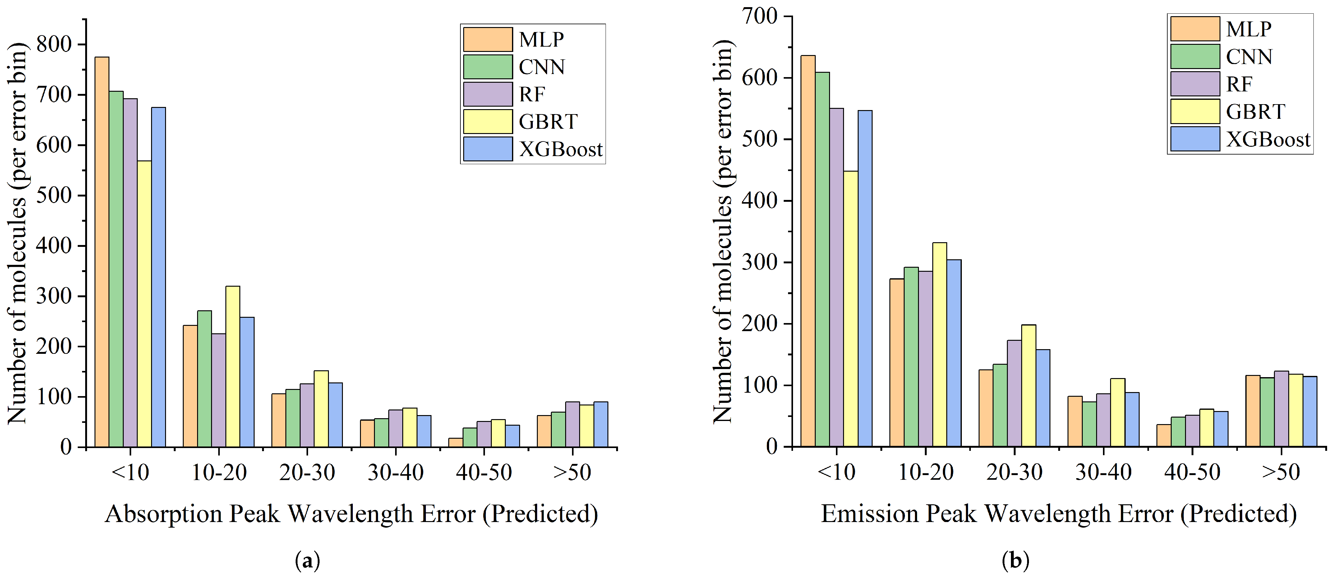
We visualized the distribution of prediction errors for all molecules, as shown in Figure 2. In each experimental round, we recorded the number of molecules within different error intervals in the corresponding test set. Upon completion of the ten-fold cross-validation, every molecule in the dataset was predicted exactly once as part of a test set, and therefore the results presented in the figure reflect the overall performance of the entire dataset during the cross-validation process. It is important to note that each round of training was carried out independently, and the molecules in the test set were not included in the corresponding training set, thereby ensuring the independence and fairness of the prediction results. It can be observed that for both the absorption peak and emission peak prediction tasks, all models exhibited their primary errors concentrated within the 10 nm range. Notably, the MLP model had the highest number of molecules in this low-error interval, indicating superior predictive accuracy and stability. In the intermediate error range of 10–30 nm, deep learning models overall showed fewer molecules than traditional machine learning models. For the high-error interval exceeding 50 nm, all models demonstrated similar prediction performance. Overall, deep learning methods not only achieved better average error metrics but also exhibited a more concentrated low-error distribution across the full error range, further confirming their advantage in molecular spectral peak prediction tasks.
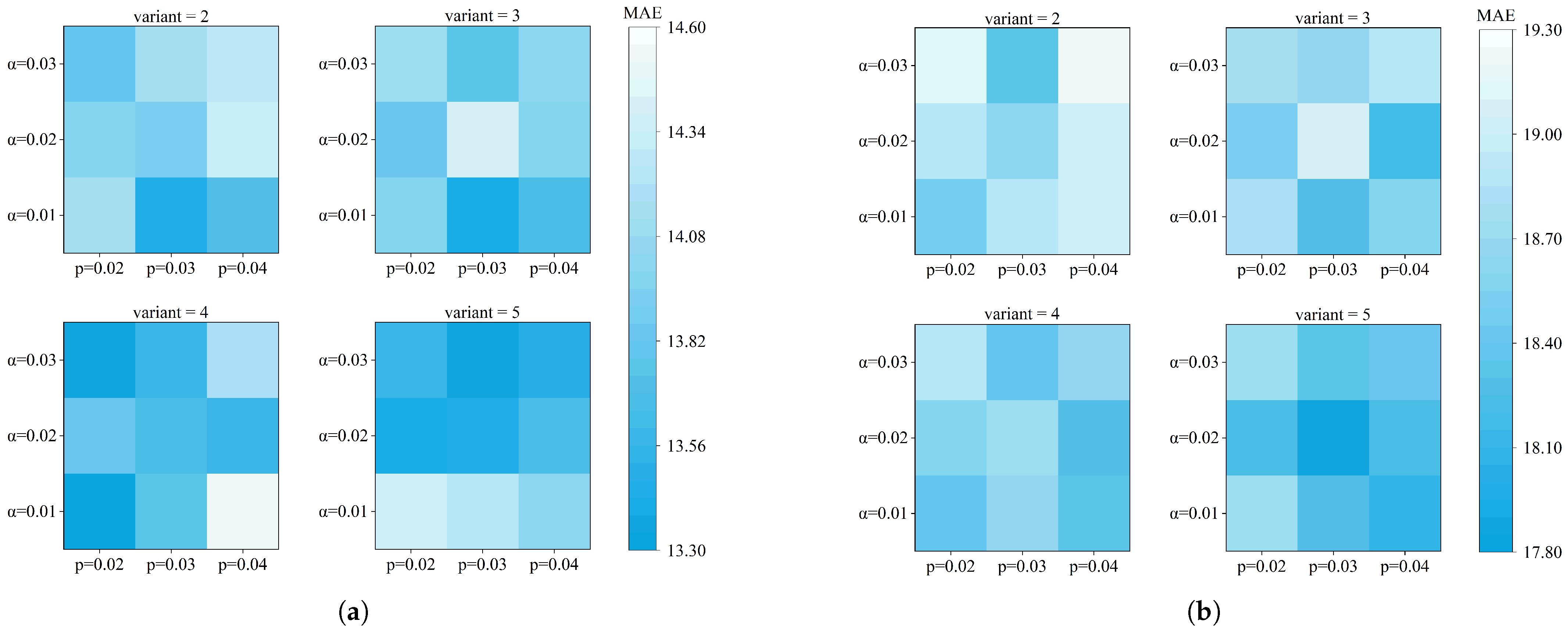
An experimental analysis was also conducted on three data augmentation hyperparameters: the number of SMILES variants, fingerprint perturbation rate p, and Gaussian noise intensity α . Specifically, we tested four values for the number of variants ( v a r i a n t = 2 ,   v a r i a n t = 3 ,   v a r i a n t = 4 ,   v a r i a n t = 5 ), three values for the fingerprint perturbation rate ( p = 0.02 ,   p = 0.03 ,   p = 0.04 ), and three values for Gaussian noise intensity ( α = 0.01 ,   α = 0.02 ,   α = 0.03 ). Using MAE as the evaluation metric, the results are presented in Figure 3.
The heatmaps indicate that the effects of p and α depend on their interaction as well as the task type. Optimal results generally appear under moderate perturbation rates with low-to-moderate noise levels, while excessive perturbation or noise tends to impair performance. As the number of variants increases, performance plateaus around variant = 3–4, suggesting that adding too many similar variants may introduce redundancy, reinforcing fixed patterns in the model and thereby limiting further improvement.
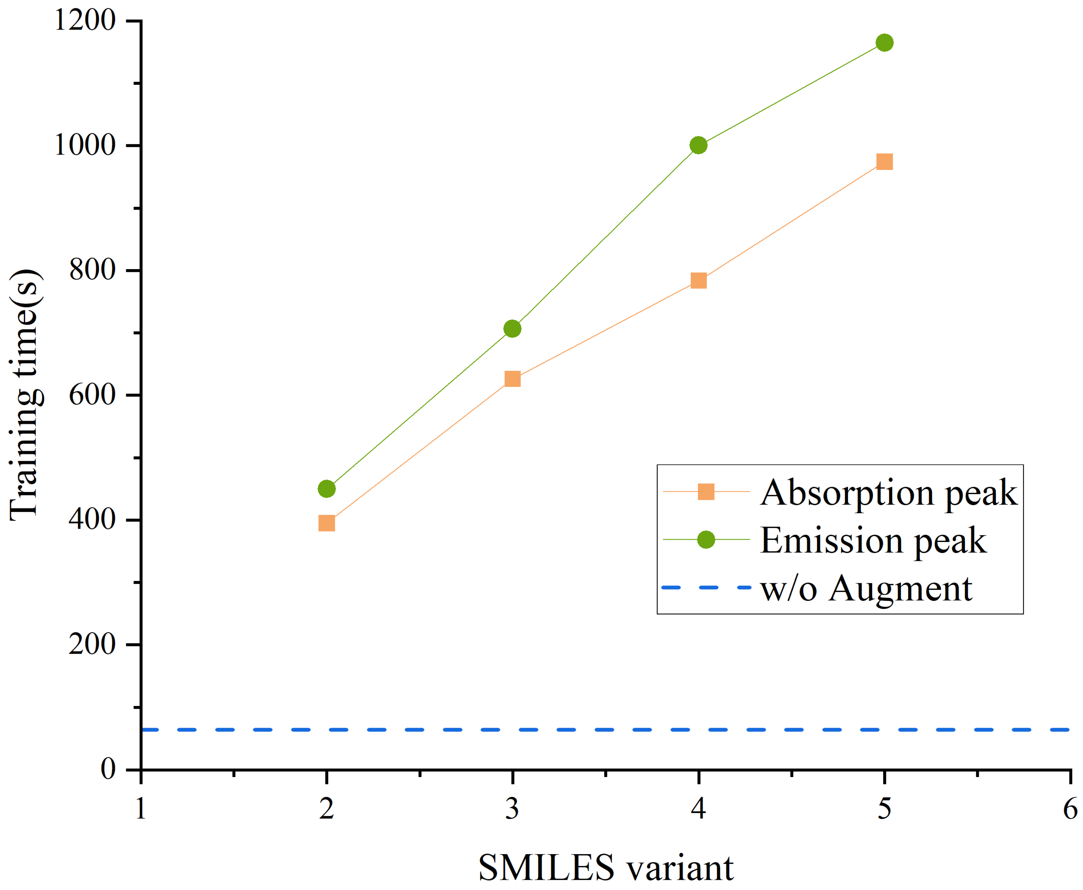
Figure 4 shows the training time required by the model under different numbers of SMILES variants, with the MLP used as the base model and consistent settings for fingerprint perturbation rate and Gaussian noise intensity. As shown in the figure, the training time increases approximately linearly with the number of SMILES variants. Notably, when the number of variants reaches 5, the training time exceeds that of the non-augmented model by more than 15-fold. This trend reflects that although the generalization ability and predictive performance of the model can be improved by introducing augmentation strategies, the computational cost and training resource requirements have also increased significantly, which may pose a bottleneck in large-scale applications or resource-constrained environments.
Let the dataset size be denoted as n, the number of augmented variants as V, the number of cross-validation folds as K, the number of training epochs as E, the batch size as B, and the computational complexity of each training step as O ( D ) . Under this setting, the time complexity of the data augmentation process is O ( n V ) , while the training time for a single epoch is O n V B · D O ( n V D ) . Consequently, the overall training complexity is O ( E n V D ) , and the total time complexity considering K-fold cross-validation becomes O ( K ( n V + E n V D ) ) O ( K E n V D ) . Therefore, it is crucial to carefully tune the data augmentation strategy to achieve an optimal balance between performance improvement and computational cost.
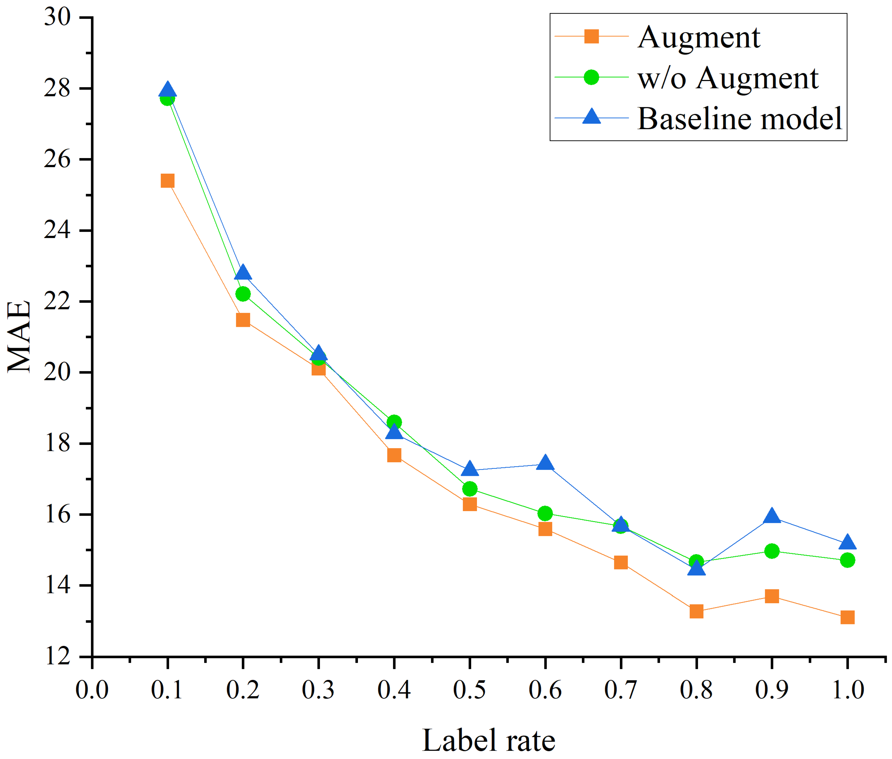
To further evaluate the model’s performance under low-data regimes, we varied the label rate of the dataset within the range 0.1 ,   0.2 ,   . . . ,   1.0 and compared three configurations: the proposed model with both energy gap features and data augmentation, the model with energy gap features but without augmentation, and a baseline model without either strategy. As shown in Figure 5, the MAE generally decreases as the label rate increases from 0.1 to 1.0, indicating that model performance improves with more labeled data. Under low label rates, both the augmented model and the energy gap-only model outperform the baseline, demonstrating stronger robustness and generalization capabilities. As the label rate exceeds 0.7, all models tend to converge in performance; however, the augmented model consistently achieves the best results across most settings. These findings collectively validate that when the amount of data is small, the introduction of data augmentation strategies and supplementary molecular electronic structure features can effectively improve performance.
In order to further validate the generalization capability of our model, we performed regression tasks on three representative datasets from the publicly available MoleculeNet benchmark [47]: ESOL, FreeSolv and Lipo. We then systematically compared our method with six mainstream methods: GCN [48], GIN [49], N-Gram [50], MolCLR [19], DGCL [51], and MDFCL [52]. RMSE was adopted as the primary evaluation metric, and the results are summarized in Table 3. As shown, our proposed model achieved a 37.14% reduction in RMSE on the ESOL dataset and a 30.37% reduction on FreeSolv. On the Lipo dataset, the model outperformed the baseline GCN by a margin of 20%. These datasets vary significantly in terms of sample size, molecular complexity, and label distribution. The consistently competitive performance across all three datasets demonstrates the robustness and generalizability of the proposed method. Notably, on FreeSolv, a dataset characterized by limited samples and high variance, the model still achieved a 30.37% reduction in RMSE., highlighting its effectiveness in small-sample scenarios. This further confirms that the incorporation of data augmentation strategies can effectively enhance the learning effect of the model.
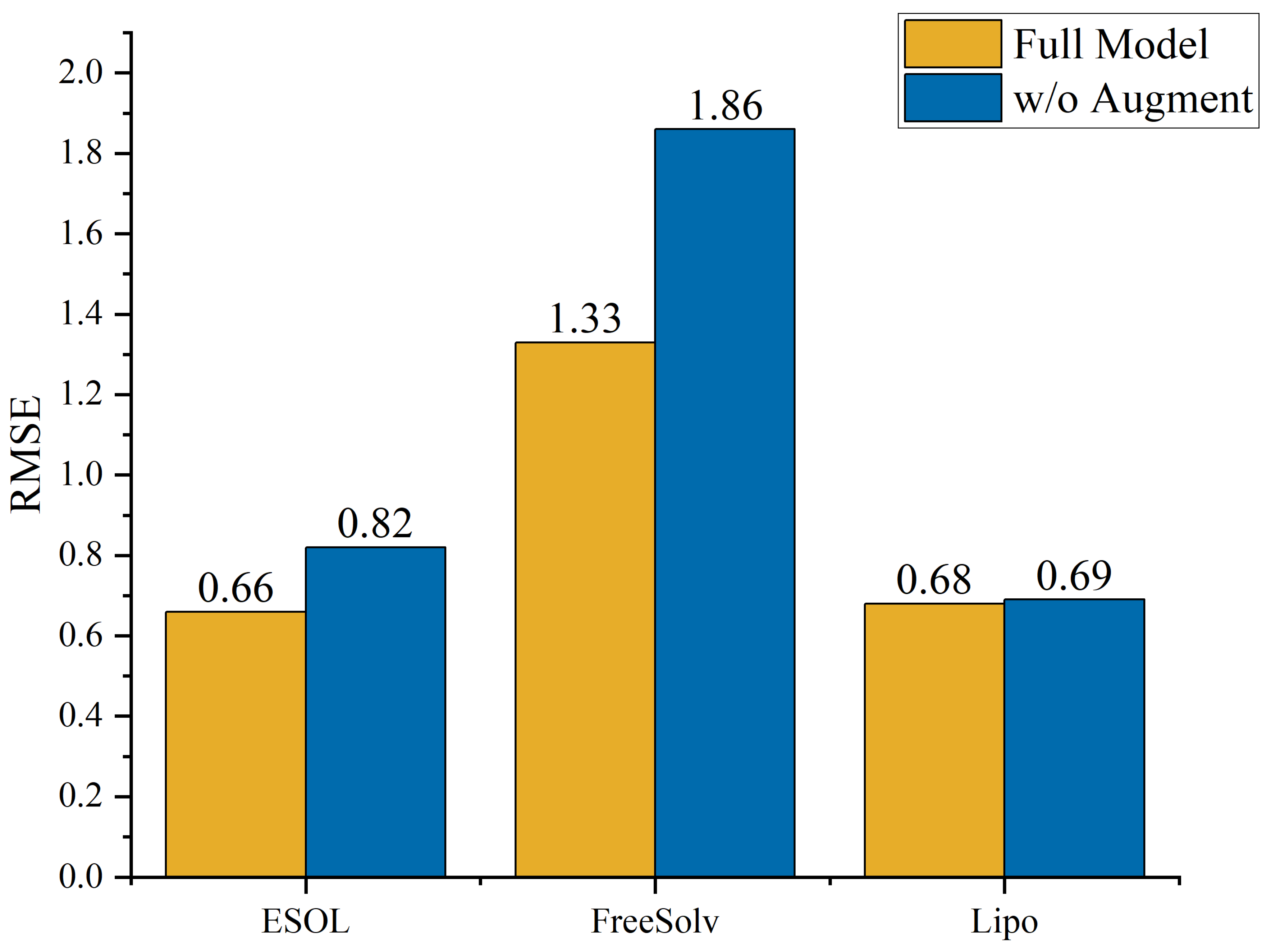
To quantify the contribution of each module to the model’s performance, ablation studies were conducted on the ESOL, FreeSolv, and Lipo datasets by removing the data augmentation component (w/o Augment), as illustrated in Figure 6. The results show that the complete model significantly outperformed its ablated counterpart in both the ESOL and FreeSolv datasets, with RMSE decreasing from 0.82 to 0.66 and from 1.86 to 1.33, respectively. These improvements underscore the critical role of data augmentation strategies in enhancing generalization under conditions of limited data or high variance. In contrast, the performance gain on the Lipo dataset was less pronounced, which may be attributed to its relatively larger sample size (4200 molecules). When the dataset size becomes large, the model can already learn stable structure–property mapping relationships from a sufficient number of samples. At this stage, even if additional data augmentation strategies or extra features are introduced, the marginal benefits gradually diminish, leading to a performance improvement that tends to plateau or even stagnate. This phenomenon is a typical example of the “performance saturation effect”. Nonetheless, the complete model still yielded superior performance. Overall, these results demonstrate not only the superiority of our method over existing methods but also its strong potential for practical applications in molecular property prediction tasks.

3.3. Ablation Study

To further evaluate and validate the effectiveness of the self-predicted molecular energy gap feature and the data augmentation strategies, an ablation study was performed using the MLP model as the primary architecture. By selectively removing the energy gap feature and the data augmentation components, performance metrics were compared under consistent model configurations and dataset conditions.
As shown in Table 4, model performance exhibited clear differences across feature configurations. Removing the energy gap feature (w/o Energy Gap) led to increased MAE values for both the absorption peak (abs) and emission peak (emi) prediction tasks, indicating that the self-predicted molecular energy gap effectively supplements electronic structure information and improves predictive accuracy. Similarly, removing the data augmentation strategies (w/o Augment) also resulted in higher MAE, demonstrating that random SMILES variant generation and bit-level noise perturbation enrich the training set’s diversity and reduce overfitting risk.
In contrast, the full model (Full Model) consistently achieved the lowest MAE across all tasks, confirming that the designed feature fusion and data augmentation strategies are both effective and complementary. Moreover, even when only data augmentation or only the energy gap feature was included, model performance surpassed that of the baseline model (Baseline Model). Overall, the ablation study validated the importance of multi-view feature fusion and data augmentation in improving spectral property prediction accuracy and model robustness, providing a methodological reference for future molecular design and property prediction tasks.

3.4. Discussion

Although this study has achieved promising results in molecular spectral property prediction, and the proposed multimodal feature fusion strategy and framework have demonstrated strong performance across multiple experiments, certain limitations remain. Specifically, the introduced HOMO/LUMO energy levels and energy gap features were derived from an external pretrained model rather than obtained directly through quantum chemical calculations. As a result, these features carry the risk of error propagation, which may become particularly pronounced under small-sample conditions. Future work could address this issue by employing high-precision computational methods such as density functional theory to calculate key molecules and construct high-quality annotated datasets. In addition, this study primarily employed shallow models which, although efficient in training, may not fully capture the complex structural characteristics of molecules, thereby limiting expressive capacity. Subsequent research could integrate graph neural networks (GNNs) and treat molecular graphs as a fourth feature view, thereby enriching the representation of molecular properties in a more comprehensive manner.

4. Conclusions

This study aims to solve the spectral prediction problem of BODIPY molecules and proposes and implements a prediction framework based on multi-view feature fusion and data augmentation strategy. A curated dataset of BODIPY compounds was constructed from the literature, and a multi-view molecular representation was developed by integrating four types of molecular fingerprints, eight physicochemical descriptors, and energy gap features predicted via a pretrained model. On this basis, a variety of models were compared horizontally. To enhance the generalization performance of the models, we introduced several data augmentation strategies, including SMILES variant generation, bit-level perturbation of molecular fingerprints, and Gaussian noise injection on target values. Experimental results demonstrate that deep learning models exhibit superior performance in handling high-dimensional features and capturing nonlinear structure–property relationships. In particular, the MLP model outperformed conventional regression methods such as RF, GBRT, and XGBoost in terms of RMSE, MAE, and R2 metrics. Moreover, ablation studies confirmed the effectiveness of the proposed molecular feature fusion and augmentation strategies. Additional generalization tests on publicly available datasets including ESOL, FreeSolv, and Lipo further validated the robustness and applicability of our method in molecular property prediction tasks.
Overall, our method demonstrates the effectiveness and scalability of multi-view feature fusion and data augmentation strategy for molecular spectral property prediction, offering a practical computational tool for the design and screening of fluorescent dye molecules.

Author Contributions

Conceptualization, X.Y., X.L., and Q.Z.; Data curation, X.L. and Q.Z.; Formal analysis, X.Y.; Investigation, X.Y. and X.L.; Methodology, X.Y. and X.L.; Resources, X.Y.; Software, X.Y. and X.L.; Supervision, Q.Z.; Validation, X.Y. and X.L.; Visualization, X.L.; Writing—original draft, X.Y. and X.L.; Writing—review and editing, X.Y., X.L., and Q.Z. All authors have read and agreed to the published version of the manuscript.

Funding

This research received no external funding.

Data Availability Statement

The pretraining data, molecular property prediction benchmarks, and the accompanying code used in this work are available in the GitHub repository at https://github.com/xuanli66/MVFDAM (accessed on 9 September 2025).

Conflicts of Interest

The authors declare no conflicts of interest.

References

  1. Medintz, I.L.; Uyeda, H.T.; Goldman, E.R.; Mattoussi, H. Quantum Dot Bioconjugates for Imaging, Labelling and Sensing. Nat. Mater. 2005, 4, 435–446. [Google Scholar] [CrossRef] [PubMed]
  2. Wolfbeis, O.S. An Overview of Nanoparticles Commonly Used in Fluorescent Bioimaging. Chem. Soc. Rev. 2015, 44, 4743–4768. [Google Scholar] [CrossRef] [PubMed]
  3. Hong, G.; Antaris, A.L.; Dai, H. Near-Infrared Fluorophores for Biomedical Imaging. Nat. Biomed. Eng. 2017, 1, 0010. [Google Scholar] [CrossRef]
  4. Uno, S.; Kamiya, M.; Yoshihara, T.; Sugawara, K.; Okabe, K.; Tarhan, M.C.; Fujita, H.; Takakura, H.; Urano, Y. A Spontaneously Blinking Fluorophore Based on Intramolecular Spirocyclization for Live-Cell Super-Resolution Imaging. Nat. Chem. 2014, 6, 681–689. [Google Scholar] [CrossRef]
  5. Mei, J.; Leung, N.L.C.; Kwok, R.T.K.; Lam, J.W.Y.; Tang, B.Z. Aggregation-Induced Emission: Together We Shine, United We Soar! Chem. Rev. 2015, 115, 11718–11940. [Google Scholar] [CrossRef]
  6. Hong, Y.; Lam, J.W.Y.; Tang, B.Z. Aggregation-Induced Emission. Chem. Soc. Rev. 2011, 40, 5361–5388. [Google Scholar] [CrossRef]
  7. Yadav, I.S.; Misra, R. Design, Synthesis and Functionalization of BODIPY Dyes: Applications in Dye-Sensitized Solar Cells (DSSCs) and Photodynamic Therapy (PDT). J. Mater. Chem. C 2023, 11, 8688–8723. [Google Scholar] [CrossRef]
  8. Loudet, A.; Burgess, K. BODIPY Dyes and Their Derivatives: Syntheses and Spectroscopic Properties. Chem. Rev. 2007, 107, 4891–4932. [Google Scholar] [CrossRef] [PubMed]
  9. Boens, N.; Leen, V.; Dehaen, W. Fluorescent Indicators Based on BODIPY. Chem. Soc. Rev. 2012, 41, 1130–1172. [Google Scholar] [CrossRef]
  10. Ni, Y.; Wu, J. Far-Red and Near Infrared BODIPY Dyes: Synthesis and Applications for Fluorescent pH Probes and Bio-Imaging. Org. Biomol. Chem. 2014, 12, 3774–3791. [Google Scholar] [CrossRef]
  11. Kamkaew, A.; Lim, S.H.; Lee, H.B.; Kiew, L.V.; Chung, L.Y.; Burgess, K. BODIPY Dyes in Photodynamic Therapy. Chem. Soc. Rev. 2013, 42, 77–88. [Google Scholar] [CrossRef] [PubMed]
  12. Zhang, J.; Wang, N.; Ji, X.; Tao, W.; Ji, S. BODIPY-Based Fluorescent Probes for Biothiols. Chem. Eur. J. 2020, 26, 4172–4192. [Google Scholar] [CrossRef]
  13. Dreuw, A.; Head-Gordon, M. Single-Reference Ab Initio Methods for the Calculation of Excited States of Large Molecules. Chem. Rev. 2005, 105, 4009–4037. [Google Scholar] [CrossRef]
  14. Tom, G.; Schmid, S.P.; Baird, S.G.; Raccuglia, P.; Aspuru-Guzik, A. Self-Driving Laboratories for Chemistry and Materials Science. Chem. Rev. 2024, 124, 9633–9732. [Google Scholar] [CrossRef] [PubMed]
  15. Sanchez-Lengeling, B.; Aspuru-Guzik, A. Inverse Molecular Design Using Machine Learning: Generative Models for Matter Engineering. Science 2018, 361, 360–365. [Google Scholar] [CrossRef]
  16. Elton, D.C.; Boukouvalas, Z.; Fuge, M.D.; Chung, P.W. Deep Learning for Molecular Design—A Review of the State of the Art. Mol. Syst. Des. Eng. 2019, 4, 828–849. [Google Scholar] [CrossRef]
  17. Noé, F.; Tkatchenko, A.; Müller, K.R.; Clementi, C. Machine Learning for Molecular Simulation. Annu. Rev. Phys. Chem. 2020, 71, 361–390. [Google Scholar] [CrossRef]
  18. Mayr, A.; Klambauer, G.; Unterthiner, T.; Hochreiter, S. Large-Scale Comparison of Machine Learning Methods for Drug Target Prediction on ChEMBL. Chem. Sci. 2018, 9, 5441–5451. [Google Scholar] [CrossRef]
  19. Wang, Y.; Wang, J.; Cao, Z.; Zhu, L.; Tang, J. Molecular Contrastive Learning of Representations via Graph Neural Networks. Nat. Mach. Intell. 2022, 4, 279–287. [Google Scholar] [CrossRef]
  20. Bajusz, D.; Rácz, A.; Héberger, K. Chemical Data Formats, Fingerprints, and Other Molecular Descriptions for Database Analysis and Searching. In Comprehensive Medicinal Chemistry III; Elsevier: Amsterdam, The Netherlands, 2017; pp. 329–378. [Google Scholar]
  21. Zhang, Y.; Fan, M.; Xu, Z.; Zhang, Y.; Tang, B.Z. Machine-Learning Screening of Luminogens with Aggregation-Induced Emission Characteristics for Fluorescence Imaging. J. Nanobiotechnol. 2023, 21, 107. [Google Scholar] [CrossRef] [PubMed]
  22. Liyaqat, T.; Ahmad, T.; Saxena, C. Advancements in Molecular Property Prediction: A Survey of Single and Multimodal Approaches. arXiv 2024, arXiv:2408.09461. [Google Scholar] [CrossRef]
  23. Huang, R.; Xia, M.; Sakamuru, S.; Zhao, J.; Shahane, S.A.; Attene-Ramos, M.; Simeonov, A.; Austin, C.P. Modelling the Tox21 10K Chemical Profiles for In Vivo Toxicity Prediction and Mechanism Characterization. Nat. Commun. 2016, 7, 10425. [Google Scholar] [CrossRef] [PubMed]
  24. Deng, J.; Yang, Z.; Wang, H.; Ojima, I.; Samaras, D.; Wang, F. A systematic study of key elements underlying molecular property prediction. Nat. Commun. 2023, 14, 6395. [Google Scholar] [CrossRef]
  25. Rogers, D.; Hahn, M. Extended-Connectivity Fingerprints. J. Chem. Inf. Model. 2010, 50, 742–754. [Google Scholar] [CrossRef] [PubMed]
  26. Niazi, S.K.; Mariam, Z. Recent Advances in Machine-Learning-Based Chemoinformatics: A Comprehensive Review. Int. J. Mol. Sci. 2023, 24, 11488. [Google Scholar] [CrossRef]
  27. Sandfort, F.; Strieth-Kalthoff, F.; Kühnemund, M.; Beecks, C.; Glorius, F. A Structure-Based Platform for Predicting Chemical Reactivity. Chem 2020, 6, 1379–1390. [Google Scholar] [CrossRef]
  28. Zeng, Y.; Qu, J.; Wu, G.; Zhang, L.; Zhang, Z.; Zhu, L.; Tang, B.Z. Two Key Descriptors for Designing Second Near-Infrared Dyes and Experimental Validation. J. Am. Chem. Soc. 2024, 146, 9888–9896. [Google Scholar] [CrossRef] [PubMed]
  29. Ramakrishnan, R.; Dral, P.O.; Rupp, M.; von Lilienfeld, O.A. Quantum Chemistry Structures and Properties of 134 Kilo Molecules. Sci. Data 2014, 1, 140022. [Google Scholar] [CrossRef]
  30. Faber, F.A.; Hutchison, L.; Huang, B.; Gilmer, J.; Schoenholz, S.S.; Dahl, G.E.; Vinyals, O.; Kearnes, S.; Riley, P.F.; von Lilienfeld, O.A. Prediction Errors of Molecular Machine Learning Models Lower than Hybrid DFT Error. J. Chem. Theory Comput. 2017, 13, 5255–5264. [Google Scholar] [CrossRef]
  31. Hu, W.; Liu, B.; Gomes, J.; Zitnik, M.; Liang, P.; Pande, V.; Leskovec, J. Strategies for Pre-Training Graph Neural Networks. In Proceedings of the International Conference on Learning Representations (ICLR), Addis Ababa, Ethiopia, 26–30 April 2020. [Google Scholar]
  32. Xia, J.; Zhu, Y.; Du, Y.; Li, S.Z. A Systematic Survey of Chemical Pre-Trained Models. In Proceedings of the 32nd International Joint Conference on Artificial Intelligence (IJCAI), Macao, China, 19–25 August 2023; pp. 6787–6795. [Google Scholar]
  33. Chithrananda, S.; Grand, G.; Ramsundar, B. ChemBERTa: Large-Scale Self-Supervised Pretraining for Molecular Property Prediction. arXiv 2020, arXiv:2010.09885. [Google Scholar]
  34. Honda, S.; Shi, S.; Ueda, H.R. SMILES Transformer: Pre-Trained Molecular Fingerprint for Low Data Drug Discovery. arXiv 2019, arXiv:1911.04738. [Google Scholar] [CrossRef]
  35. Shorten, C.; Khoshgoftaar, T.M. A Survey on Image Data Augmentation for Deep Learning. J. Big Data 2019, 6, 60. [Google Scholar] [CrossRef]
  36. Yang, S.; Xiao, W.; Zhang, M.; Guo, S.; Zhao, J.; Shen, F. Image Data Augmentation for Deep Learning: A Survey. arXiv 2022, arXiv:2204.08610. [Google Scholar]
  37. Wei, J.; Zou, K. EDA: Easy Data Augmentation Techniques for Boosting Performance on Text Classification Tasks. In Proceedings of the 2019 Conference on Empirical Methods in Natural Language Processing and the 9th International Joint Conference on Natural Language Processing (EMNLP-IJCNLP), Hong Kong, China, 3–7 November 2019; pp. 6382–6388. [Google Scholar]
  38. Wang, S.; Guo, Y.; Wang, Y.; Sun, H.; Huang, J.; Tang, J. SMILES-BERT: Large Scale Unsupervised Pre-Training for Molecular Property Prediction. In Proceedings of the 10th ACM International Conference on Bioinformatics, Computational Biology and Health Informatics, Niagara Falls, NY, USA, 7–10 September 2019; pp. 429–436. [Google Scholar]
  39. Eraqi, B.A.; Khizbullin, D.; Nagaraja, S.S.; Gao, L.; Aspuru-Guzik, A. Molecular Property Prediction in the Ultra-Low Data Regime. Commun. Chem. 2025, 8, 201. [Google Scholar] [CrossRef] [PubMed]
  40. Li, C.; Feng, J.; Liu, S.; Hu, X.; Wang, J.; Tang, J. A Novel Molecular Representation Learning for Molecular Property Prediction with a Multiple SMILES-Based Augmentation. Comput. Intell. Neurosci. 2022, 2022, 8464452. [Google Scholar] [CrossRef] [PubMed]
  41. Rumelhart, D.E.; Hinton, G.E.; Williams, R.J. Learning Representations by Back-Propagating Errors. Nature 1986, 323, 533–536. [Google Scholar] [CrossRef]
  42. LeCun, Y.; Bottou, L.; Bengio, Y.; Haffner, P. Gradient-Based Learning Applied to Document Recognition. Proc. IEEE 1998, 86, 2278–2324. [Google Scholar] [CrossRef]
  43. Breiman, L. Random Forests. Mach. Learn. 2001, 45, 5–32. [Google Scholar] [CrossRef]
  44. Friedman, J.H. Greedy Function Approximation: A Gradient Boosting Machine. Ann. Stat. 2001, 29, 1189–1232. [Google Scholar] [CrossRef]
  45. Chen, T.; Guestrin, C. XGBoost: A Scalable Tree Boosting System. In Proceedings of the 22nd ACM SIGKDD International Conference on Knowledge Discovery and Data Mining, San Francisco, CA, USA, 13–17 August 2016; pp. 785–794. [Google Scholar]
  46. Kohavi, R. A Study of Cross-Validation and Bootstrap for Accuracy Estimation and Model Selection. In Proceedings of the 14th International Joint Conference on Artificial Intelligence (IJCAI), Montreal, QC, Canada, 20–25 August 1995; pp. 1137–1145. [Google Scholar]
  47. Wu, Z.; Ramsundar, B.; Feinberg, E.N.; Gomes, J.; Geniesse, C.; Pappu, A.S.; Leswing, K.; Pande, V. MoleculeNet: A Benchmark for Molecular Machine Learning. Chem. Sci. 2018, 9, 513–530. [Google Scholar] [CrossRef]
  48. Kipf, T.N.; Welling, M. Semi-Supervised Classification with Graph Convolutional Networks. In Proceedings of the 5th International Conference on Learning Representations (ICLR), Toulon, France, 24–26 April 2017. [Google Scholar]
  49. Xu, K.; Hu, W.; Leskovec, J.; Jegelka, S. How Powerful Are Graph Neural Networks? In Proceedings of the International Conference on Learning Representations (ICLR), New Orleans, LA, USA, 6–9 May 2019. [Google Scholar]
  50. Liu, S.; Demirel, M.F.; Liang, Y. N-Gram Graph: Simple Unsupervised Representation for Graphs, with Applications to Molecules. Adv. Neural Inf. Process. Syst. 2019, 32, 8464–8476. [Google Scholar]
  51. Jiang, X.; Tan, L.; Zou, Q. DGCL: Dual-Graph Neural Networks Contrastive Learning for Molecular Property Prediction. Briefings Bioinform. 2024, 25, bbae474. [Google Scholar] [CrossRef] [PubMed]
  52. Gong, X.; Liu, M.; Liu, Q.; Li, X.; Chen, G.; Tang, J. MDFCL: Multimodal Data Fusion-Based Graph Contrastive Learning Framework for Molecular Property Prediction. Pattern Recognit. 2025, 163, 111463. [Google Scholar] [CrossRef]
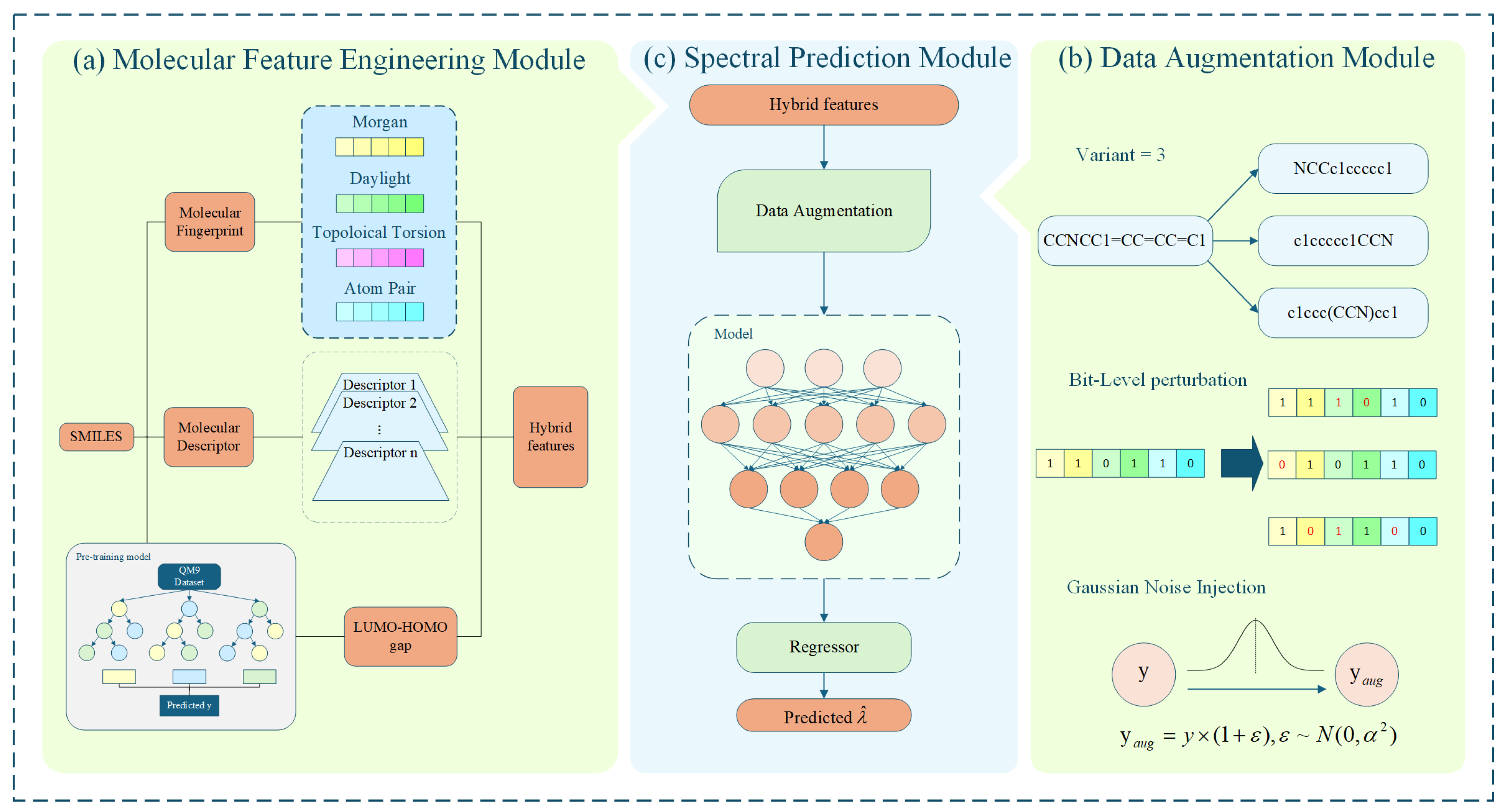
Figure 1. Overall framework of the proposed method. (a) Molecular Feature Engineering Module. The lower-left pre-trained model illustrates the regression learning process performed with the XGBoost model on the QM9 dataset. The tree structure represents the ensemble of decision trees, and each box corresponds to the intermediate prediction output of an individual tree. The y value denotes the predicted molecular energy gap. (b) Data Augmentation Module, in this module, y represents the target value that requires augmentation, y a u g denotes the augmented value, and variant indicates the number of generated variants. (c) Spectral Prediction Module, where λ represents the molecular absorption/emission wavelength predicted by this module.
Mathematics 13 02947 g001
Figure 2. Distribution of model prediction errors, where the x-axis represents the prediction error intervals of molecules and the y-axis indicates the number of molecules within each interval. (a) The error molecule distribution for the absorption peak prediction task. (b) The error molecule distribution for the emission peak prediction task.
Mathematics 13 02947 g002
Figure 3. Effect of data augmentation hyperparameters on model prediction. Here, α denotes the Gaussian noise amplitude, p represents the fingerprint perturbation rate, and v a r i a n t indicates the number of generated variants. (a) The results illustrate the predictive performance for absorption peak estimation under these conditions. (b) The results illustrate the predictive performance for emission peak estimation under these conditions.
Mathematics 13 02947 g003
Figure 4. The training time of the model under different numbers of SMILES variants, with the horizontal line indicating the training time of the model without augmentation.
Mathematics 13 02947 g004
Figure 5. Comparison of MAE under different label rates for three models on absorption peak prediction.
Mathematics 13 02947 g005
Figure 6. Comparison of RMSE between the full model and the ablated version without data augmentation on ESOL, FreeSolv, and Lipo datasets, demonstrating the benefit of data augmentation.
Mathematics 13 02947 g006
Table 1. Sample sizes under different conditions.
Augmented VariantsTraining SamplesTest Samples
variant = 0 11141127
variant = 23423127
variant = 34564127
variant = 45705127
variant = 56846127
1 When variant = 0, no data augmentation is applied, and the training and test set sizes remain equal to the original dataset partition.
Table 2. Performance comparison of models. The best performance in each column is highlighted in bold.
ModelAbsorption PeakEmission Peak
MAERMSER2MAERMSER2
MLP15.18 ± 2.6323.28 ± 4.020.898 ± 0.03219.34 ± 1.7029.42 ± 3.010.837 ± 0.034
Ours-MLP13.11 ± 2.0222.11 ± 3.910.908 ± 0.03018.09 ± 1.7328.95 ± 2.620.842 ± 0.030
CNN16.47 ± 4.3524.57 ± 5.230.884 ± 0.04920.54 ± 3.2829.82 ± 2.270.833 ± 0.025
Ours-CNN14.56 ± 2.3123.46 ± 3.960.896 ± 0.03118.64 ± 1.4629.48 ± 3.100.836 ± 0.035
RF17.42 ± 1.7426.27 ± 2.410.872 ± 0.02421.21 ± 1.8630.50 ± 3.180.824 ± 0.038
Ours-RF16.23 ± 1.8926.43 ± 3.070.870 ± 0.03119.84 ± 1.6830.44 ± 3.080.825 ± 0.037
GBRT17.96 ± 1.5926.17 ± 2.530.873 ± 0.02521.76 ± 1.5730.53 ± 2.570.824 ± 0.031
Ours-GBRT17.44 ± 1.8425.70 ± 2.860.877 ± 0.02721.40 ± 1.4830.34 ± 2.480.827 ± 0.029
XGBoost16.93 ± 2.4126.11 ± 3.200.874 ± 0.03020.53 ± 1.7629.82 ± 2.530.830 ± 0.028
Ours-XGBoost16.34 ± 2.0525.81 ± 3.560.876 ± 0.03119.77 ± 1.4529.56 ± 2.640.836 ± 0.031
Table 3. Regression performance (RMSE) of different models on the ESOL, FreeSolv, and Lipo datasets. Lower RMSE indicates better performance. The best performance in each column is highlighted in bold.
ModelRMSE
ESOLFreeSolvLipo
GCN1.43 ± 0.052.87 ± 0.140.85 ± 0.08
GIN1.45 ± 0.022.76 ± 0.180.85 ± 0.07
N-Gram1.10 ± 0.032.51 ± 0.190.88 ± 0.12
MolCLR1.11 ± 0.012.20 ± 0.200.65 ± 0.08
DGCL1.01 ± 0.021.91 ± 0.25 0 . 48 ± 0 . 03
MDFCL1.05 ± 0.052.44 ± 0.230.68 ± 0.03
Ours-MLP 0 . 66 ± 0 . 06 1 . 33 ± 0 . 14 0.68 ± 0.03
Table 4. Ablation study results for the model, with MAE as the evaluation metric.
Modelw/o Energy Gapw/o AugmentBaseline ModelFull Model
AbsEmiAbsEmiAbsEmiAbsEmi
MLP13.86 ± 2.3218.24 ± 1.7314.71 ± 2.4319.32 ± 1.4015.18 ± 2.6319.34 ± 1.7013.11 ± 2.0218.09 ± 1.73
CNN14.89 ± 1.7419.20 ± 1.3215.04 ± 2.0020.11 ± 1.7316.47 ± 4.3520.54 ± 3.2814.56 ± 2.3118.64 ± 1.46
RF16.03 ± 1.8419.87 ± 1.7117.51 ± 1.7921.30 ± 1.7817.42 ± 1.7421.21 ± 1.8616.23 ± 1.8919.84 ± 1.68
GBRT17.82 ± 1.9321.30 ± 1.7817.81 ± 1.7921.60 ± 1.6117.96 ± 1.5921.76 ± 1.5717.44 ± 1.8421.40 ± 1.48
XGBoost16.31 ± 2.0619.54 ± 1.2615.91 ± 2.0919.31 ± 1.6316.34 ± 2.0519.77 ± 1.4515.82 ± 1.8519.26 ± 1.50
Disclaimer/Publisher’s Note: The statements, opinions and data contained in all publications are solely those of the individual author(s) and contributor(s) and not of MDPI and/or the editor(s). MDPI and/or the editor(s) disclaim responsibility for any injury to people or property resulting from any ideas, methods, instructions or products referred to in the content.