Article

Optimizing Commercial Teams and Territory Design Using a Mathematical Model Based on Clients’ Values: A Case Study in Canada

1
Nors Group, S.A., 4149-010 Porto, Portugal
2
Banco Português de Investimento, 1050-094 Lisboa, Portugal
3
LEMA, ISEP, Polytechnic of Porto, rua Dr. António Bernardino de Almeida, 4249-015 Porto, Portugal
4
CEOS.PP, ISCAP, Polytechnic of Porto, rua Jaime Lopes Amorim, 4465-004 São Mamede de Infesta, Portugal
*
Authors to whom correspondence should be addressed.
These authors contributed equally to this work.
Mathematics 2025, 13(18), 2940; https://doi.org/10.3390/math13182940
Submission received: 5 July 2025 / Revised: 2 September 2025 / Accepted: 6 September 2025 / Published: 11 September 2025
(This article belongs to the Special Issue Advances in Control Theory and Optimizations)

Abstract

This study, set in Nors Construction Equipment ST in Canada, addresses logistical challenges by enhancing commercial team evaluation and market sectorization. Traditional performance assessments relied only on sales, lacking other efficiency measures. This research proposes a mathematical function to combine diverse Key Performance Indicators (KPIs) to better evaluate team effectiveness. Additionally, it aims to optimize the sales territory assignment, improving resource allocation across Canada’s expansive, sparsely populated regions. Customer segmentation was conducted using the RFM model, classifying clients into Low-, Mid-, and High-Value groups based on purchasing behavior. For incorporating multiple KPIs in the evaluation of commercial teams’ performance, the Analytic Hierarchy Process (AHP) was used. Sectorization was modeled as a linear programming problem to minimize travel distances while ensuring compact sales territories. Constraints included balancing sales opportunities and customer types across assigned territories. As a result, the proposed optimization model significantly improves operational efficiency through better-balanced sales territories and reduced travel. Improved sectorization enhances market penetration and customer coverage, which is expected to lead to increased sales and support the company’s growth objectives. The mathematical models developed in this study allowed for a deeper understanding of the performance and provided management with tools to refine sales strategies and allocate resources more effectively. The article ends with a discussion on the possibility of ChatGPT being used to replace a mathematician in performing this analysis for the company. It was observed that ChatGPT (version GPT-4o) provided an extremely incomplete solution, evaluating the commercial teams solely based on profit and sales and not addressing the sectorization problem at hand.

1. Introduction

Efficient sectorization of commercial teams is imperative for companies seeking to optimize their sales performance and maximize customer engagement. In the case of the company used in this study, Nors Construction Equipment Canada ST, the sectorization of its commercial teams poses a significant challenge. The objective of this work is to address this challenge by determining the optimal mix of customer allocation and geographical coverage for commercial teams, with a focus on ensuring equitable opportunities between teams.
This study utilizes advanced optimization techniques, specifically focusing on formulating the sectorization challenge as a linear programming problem. Additionally, the RFM (Recency, Frequency, Monetary) model is employed to assess the value of each client. To balance opportunities among commercial teams, an optimization model leveraging the RFM-derived client value classification is used. By integrating these methodologies, the aim is to develop a sectorization plan that not only enhances sales effectiveness but also optimizes resource allocation within the company. For practical implementation, the pyscipopt package (version 5.6.0) in Python (version 3.12.0) was employed, which serves as an interface to the SCIP (Solving Constraint Integer Programs) solver [1,2].
In Portugal, jobs for mathematicians inside business companies are hard to find. Many companies are small and family-owned and are still taking the first steps in academia–industry collaboration. The Nors group is an exception that employs several mathematicians because the company understands that a mathematician with skills in modeling, simulation, and optimization is a valuable asset in their permanent staff and can bring the company one step ahead. But, with the advent of artificial intelligence (AI) and Large Language Model (LLM) massification, people may be led to think that any data analysis can be performed by AI without having sophisticated math skills. Therefore, the last objective of this research work was to compare our findings to the outputs ChatGPT provides when prompted with the exact same task, in order to assess if an LLM based on AI can replace a mathematician by reaching the same results when given the same initial information.
Subsequent sections will explore the specifics of the mathematical approach, present the findings, and discuss the results.

2. Definitions and Generalities

This section will introduce the RFM (Recency, Frequency, Monetary) model, the sectorization problem and optimization techniques, as well as some concepts needed for the developed solution.

2.1. Assessing a Client’s Value with the RFM Model

The RFM model (Recency, Frequency, and Monetary Value) is an analytical approach aimed at segmenting customers based on their purchasing behavior, dividing them into various groups. This model allows for analyzing how recently a customer made a purchase (recency), how many transactions they have made in a specific period of time (frequency), and how much they have spent (monetary value) [3].
RFM can help to identify valuable customers and develop an effective marketing strategy [4]. RFM is widely used in direct marketing for simplicity of use, implementation, and interpretability of its results [5,6]. Extensions of the traditional RFM model include stochastic variants to estimate the customer value [7], the addition of new evaluation dimensions, such as the cost-to-serve [8], the product perspective [9], or the information related to the product catalog [10], or a combination of other methods. The RFM model combined with data mining can reveal useful hidden patterns in customer segments [11] and extract user purchase behavior features [12]. Combined with formal concept analysis, it can build a knowledge structure to simultaneously offer marketers customer segmentation and relationships in customer data [13].
The first variable, recency (R), represents the time elapsed since the last time the customer made a purchase from the company. It refers to the time interval measured in a given timescale (e.g., days, months, years) since the last purchase. Many marketing professionals consider that there is a inverse relationship between recency and response rate: customers who made purchases more recently are more likely to make another purchase. However, the specific relationship between recency and purchase clearly depends on various factors, such as the business sector [14].
Frequency (F) represents how many times a customer made purchases within a certain period of time. Generally, it is measured as the number of purchase occasions since the first acquisition. In order to adjust to the customer’s longevity, the number of purchase occasions can be divided by the duration of the customer relationship. Similar to recency, the exact relationship between frequency and response rates must be determined empirically. However, the relationship is often positive: customers who frequently purchase a product are more likely to respond [14].
Monetary value (M) represents the value of previous purchases. It can be measured as the amount of money spent during a certain period of time. Alternatively, one can use the total amount divided by the duration of the customer relationship or simply the average spending per order. Similarly to frequency, the monetary value tends to have a positive relationship with the probability of response [14].
Once the information about the customers’ purchasing records is summarized into the three RFM variables, a model is constructed to predict the response propensity of each customer. The RFM variables are discretized in a scale of 5 to 1, where the top quintile is given a score of 5, as proposed by [15]. More specifically, three separate codes are created for each variable. For example, customers are classified according to their recency. A code of 5 is assigned to customers with the most recent transactions, representing the top 20% of recency values. Customers with recency values within the next 20% receive a code of 4, and so on. As a result, each customer receives a recency code of 5, 4, 3, 2, or 1. In other words, the continuous variable (recency) has been transformed into five discrete variables (recency codes). Similarly, a frequency code and a monetary code are assigned to each customer. As a result, each customer is now represented by three RFM codes [14]. The threshold of 20 % is inspired by the Pareto principle [16], which states that 80 % of a business’s revenues come from around 20 % of its clients [17]. Segmenting customers using a simple rule-based clustering method with predefined value thresholds like this is common in the literature [18]. Other popular possibilities of segmenting the customers using the RFM variables are using K-means algorithms, hierarchical clustering methods, and latent class models, among others. A known weakness of the RFM model is its fairness in differentiating old customers that have decreased or stopped their purchases and new customers that have just started buying [19]. In the business scope of selling heavy machinery and construction equipment, there are many high-volume sales that are not frequent, or even recent, but still represent valuable customers that may not be lost. Therefore, the company considered the three dimensions of the RFM model equally important. For this reason, the codes for each variable are summed to give the RFM Score. RFM Score can be used as a proxy for an important direct marketing concept, lifetime value, which is the expected net profit a customer will contribute to a business over the period of time a customer remains a customer. High-RFM customers represent future business potential because the customers are more likely to buy again and have a high lifetime value. Low-RFM customers represent less of a business opportunity and low lifetime value [3]. Following this idea, clients were grouped into three categories: Low-Value, Mid-Value, and High-Value. These groups are obtained by dividing the RFM Score into three quantiles, so that each group has approximately the same number of clients (the Low-Value group consists of clients with the lowest RFM Scores). The resulting three groups of the RFM model will be used when determining the optimal geographical coverage for commercial teams, to achieve a more balanced customer allocation.

2.2. Sectorization Problems

Sectorization problems (SPs) consist of dividing a whole (often a geographical area) into smaller parts, respecting a set of constraints and aiming to achieve specific objectives [20]. In the literature, they are also known as Territory Design or Districting Problems [21]. The concept of basic units (BUs) is used, which refers to the smaller areas that make up the territory and are considered indivisible. Thus, sectorization can be seen as the division into k parts ( S 1 , S 2 , …, S k ) of a certain number n of Basic Units (BUs) that form a set V = B U 1 , B U 2 , , B U n . Each sector S i , i 1 , , k , is defined by
S i = j = 1 n i B U i j
where B U i j is the j-th basic unit of sector i, such that
i = 1 k S i = V , S i S j = ( i j ) e j = 1 k n j = n
Although any partition of V is a feasible solution, i.e., a solution that satisfies all constraints, for a sectorization problem, these problems often require the solution to be ‘good’ with respect to one or several criteria.
The sectors are built while taking into consideration various criteria [21], where two very common ones are as follows:
  • Compactness: sectors should have geographically concentrated activity; according to the problem scenario, higher density in the sectors means less travel, greater accessibility, and more time available for sales or services.
  • Balance: sectors should be balanced with respect to a certain measure of activity, containing similar parts of the whole.
These two criteria are very important, given the specificity of the business and the operational context of Canada. Matching the workload in each territory with the capacity of its full-time salespeople is known to produce higher sales [22]. Canada is a very large country, and the distance between clients can be a challenge for salespeople to cover. Also, in the business of construction equipment and heavy machinery, sales teams must cover many different types of clients. Hence, the company wanted their sales territories to be more compact and also more balanced, to increase the fairness of sales opportunities.
Sectorization problems arise in different contexts and have wide-ranging applications. Examples of common areas where these problems are applied include public management (health [23], public transportation [24], policing [25], and education [26]), commerce (definition of sales territories [27], product distribution [28], and customer satisfaction [29]), and logistics (storage, distribution [30], and many vehicle routing problems [31]). In these works, the methods used to tackle sectorization problems vary from exact approaches to metaheuristics methods. Although metaheuristics are very fast and suitable for large-scale problems, they do not guarantee an optimal solution and results can vary between runs. In this paper, the size of the instances is moderate and the problem is well structured; therefore, an integer programming model was used to guarantee the optimality of the solutions, interpretability of constraints and parameters, as well as its transparency and rigor.

2.3. Pareto Front

When dealing with more than one objective function, as is usual in sectorization problems, different optimal solutions can be compared through a Pareto front.
Let S be the space of feasible solutions and N 2 be the number of objective functions. The Pareto front is built based on the concept of dominance: a solution in the objective space u = ( u 1 , u 2 , , u N ) dominates (Pareto-dominates) another one v = ( v 1 , v 2 , , v N ) if and only if i 1 , 2 , , N : u i v i and i 1 , 2 , , N : u i < v i . A solution y S is a Pareto optimal solution if and only if x S , y is not dominated by x. The Pareto set is the set of all Pareto optimal solutions in S for a certain problem. The Pareto front is the image of this set in the objective space [20].
The Pareto front approach was selected to explicitly model the trade-offs between conflicting objectives, offering a diverse set of optimal solutions without the need to impose subjective weightings upfront, like weighted-sum methods obliging. It supports post-optimization decision-making, empowering stakeholders to evaluate and select from a set of optimal trade-offs based on situational priorities or domain knowledge. Providing a decision-maker with several Pareto optimal solutions can help them to consider a wide range of management options based on robust information.

3. Model Formulation

The extensive utilization of mixed-integer linear programs (MILs) in conjunction with the efficacy of MILP solvers, when integrated within software-based decision support systems, has been demonstrated to significantly enhance organizational planning [32]. In this section, a mathematical model is presented to find a commercial team sectorization suitable for the company’s needs, i.e., to optimize geographic areas and clients per commercial team, considering equality of opportunities. To achieve this, the optimization problem will be modeled with integer linear programming. Subsequently, this model will be implemented in Python and compared with the current sectorization of the teams.

3.1. Sets and Parameters

In this problem, the following indexes, sets, and parameters are defined in Table 1.
In this case study, ‘V’ represents the total set of customers under study, and ‘C’ will be the set of commercial teams to be assigned to each customer.
The subsets L, M, and H were obtained through the RFM model, using the logic mentioned at the end of the Section 2.1. The parameter n v was calculated by counting the opportunities for each customer v. Subsequently, the average number of opportunities, relative to Low-Value customers, was determined by summing the opportunities for customers in group L and dividing by the number of workers, i.e., μ l = v L n v c C s c . The same logic was applied for Mid-Value and High-Value customers, with the formulas μ m = v M n v c C s c and μ h = v H n v c C s c , respectively.
The tolerance ( τ > 0 ) is the value by which the weighted average of the number of opportunities assigned to each commercial team is allowed to vary. The outcome of this model heavily depends on the value assigned to the parameter τ .

3.2. Decision Variables

The decision variables of this model are binary and defined as
x c v = 1 if   customer   v   is   assigned   to   commercial   team   c ; 0 otherwise .
These decision variables can be described as the partition of the set ‘V’, customers, into a number ‘k’ of commercial teams that satisfy the specified planning criteria.

3.3. Objective Function

The objective of this problem is to find the most compact division for the company considering the geographical dimension of Canada. Therefore, it is defined as minimizing the total distance from the customers to the commercial teams, that is,
min v V c C d c v x c v
The use of distance in the objective function aims to satisfy the criterion of compactness. The company aims for a multi-objective solution, as it not only prioritizes compact sectors but also prefers solutions balanced in terms of opportunities for the commercial teams. It was decided to incorporate the balance criterion as a constraint, as will be seen next.

3.4. Constraints

After establishing the objective function, it is necessary to define the conditions that lead to a solution that makes sense and meets the real requirements imposed by the company.
Therefore, the constraints of this problem are enumerated as follows:
c C x c v = 1 v V
v V x c v 1 c C
μ l × s c × ( 1 τ ) v L x c v n v μ l × s c × ( 1 + τ ) c C
μ m × s c × ( 1 τ ) v M x c v n v μ m × s c × ( 1 + τ ) c C
μ h × s c × ( 1 τ ) v H x c v n v μ h × s c × ( 1 + τ ) c C
x c v { 0 , 1 } c C , v V
Constraint (2) ensures that each customer must be assigned to exactly one commercial team.
Constraint (3) ensures that each commercial team must have at least one customer.
Inspired in the models presented in [33,34], constraints (4), (5), and (6) aim to satisfy the criterion of balance: constraint (4) reflects the balance in terms of the number of opportunities for commercial teams regarding Low-Value customers, while constraints (5) and (6) address Mid- and High-Value customers, respectively. This ensures that the commercial teams are balanced not only in terms of the number of opportunities but also in terms of the type of assigned customers.

4. Results

To assess the commercial performance of the teams, the company used only sales, which was a poor approach, and wanted to consider more Key Performance Indicators (KPIs) to evaluate the sales teams (such as the number of sales opportunities, the percentage of lost and won opportunities per worker, the monetary value of the lost and won contracts, etc). The Analytic Hierarchy Process (AHP) is a multi-criteria decision-making methodology that allows complex and multifaceted problems to be addressed, providing a framework for evaluating and comparing alternatives in relation to different criteria [35,36]. The AHP has recently been applied to automotive after-sales services [37], adoption of electrical vehicles [38], garage equipment purchasing decisions [39], efficient inventory policies for hardware goods and construction materials [40], and to quantify risks in the supply chain [41]. In this work, the AHP was used to obtain a comprehensive and thorough evaluation of the construction equipment sales teams. Through pairwise comparisons, the company managers judged the importance of each KPI. This produced a comparison matrix, which was validated with a consistency ratio of CR = 0.099, within the limit of 0.10 [42]. The eigenvalues of the matrix provide the weights to be used for each KPI in a final score function that evaluates each team. By measuring the performance of teams with this score function that combines several KPIs, and also analyzing all KPIs individually, management can better understand why some large-equipment sales contracts are being lost and can take actions to prevent losses and increase sales by using their teams in the best possible way.
To define the new Territory Design for the commercial teams, the optimization model was implemented using the PySCIPOpt package (version 5.6.0) in Python (version 3.12.0) on a computer with a 13th Gen Intel(R) Core(TM) i5-1335U at 1.30 GHz and 16 GB RAM. PySCIPOpt serves as a Python interface to the SCIP optimization solver, enabling users to tackle mixed-integer linear and nonlinear programming challenges directly within Python scripts.
For solving the model, multiple values of τ were considered, in order to find the best solution for the problem. Figure 1 shows how the balance and compactness metrics vary across different values of τ (from 0.1 to 1.0). In this figure, a Pareto front related to the distance required by the commercial teams to visit all clients versus the unbalance indicator of the sets of clients for different tolerance values is presented, where each plotted point is the solution for each τ value.
The unbalance value is given by
c C v V n v × x c v ( μ l + μ m + μ h ) × s c 1
This represents how much the commercial team is unbalanced in terms of opportunities. A higher value indicates a larger unbalance.
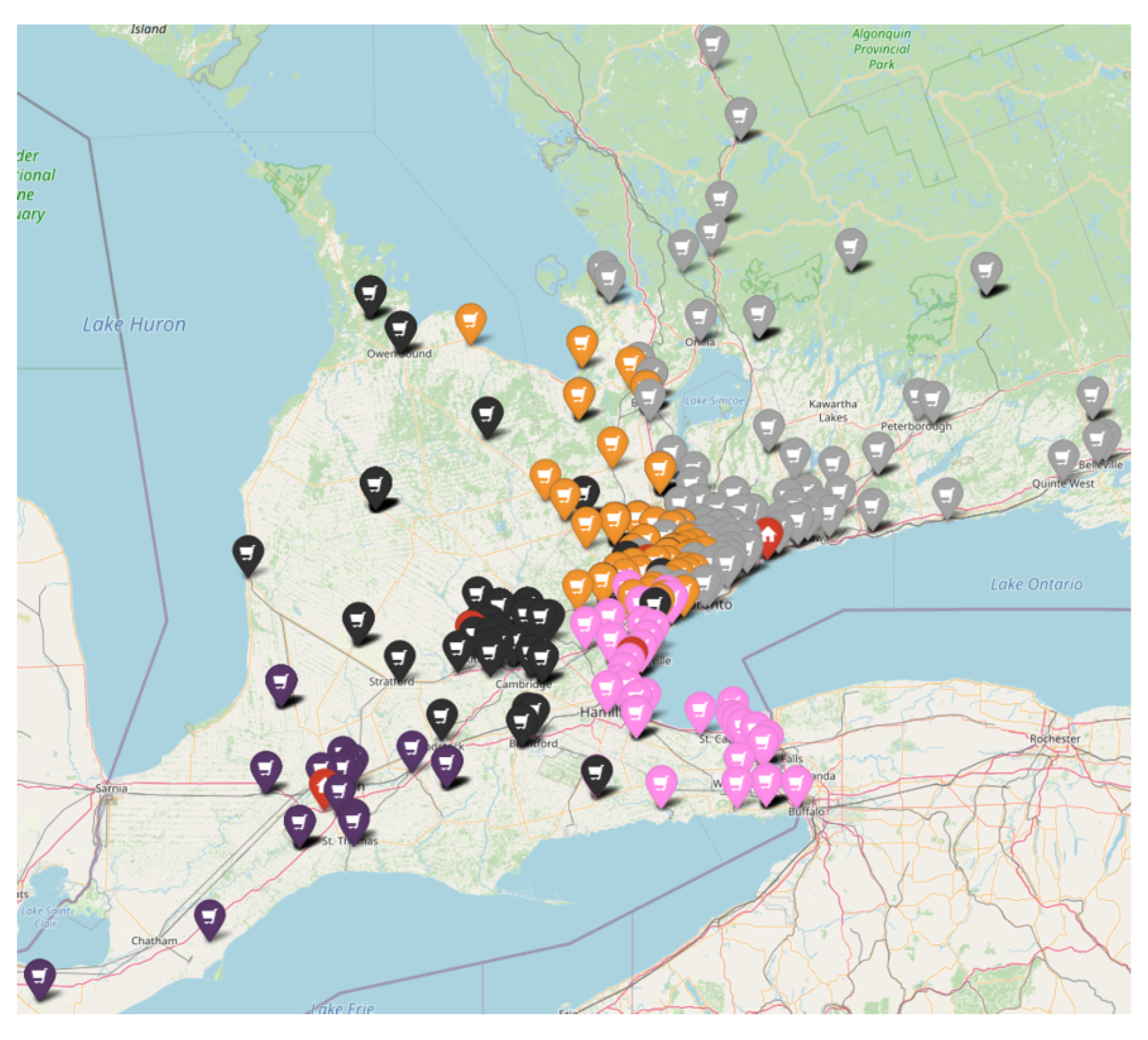
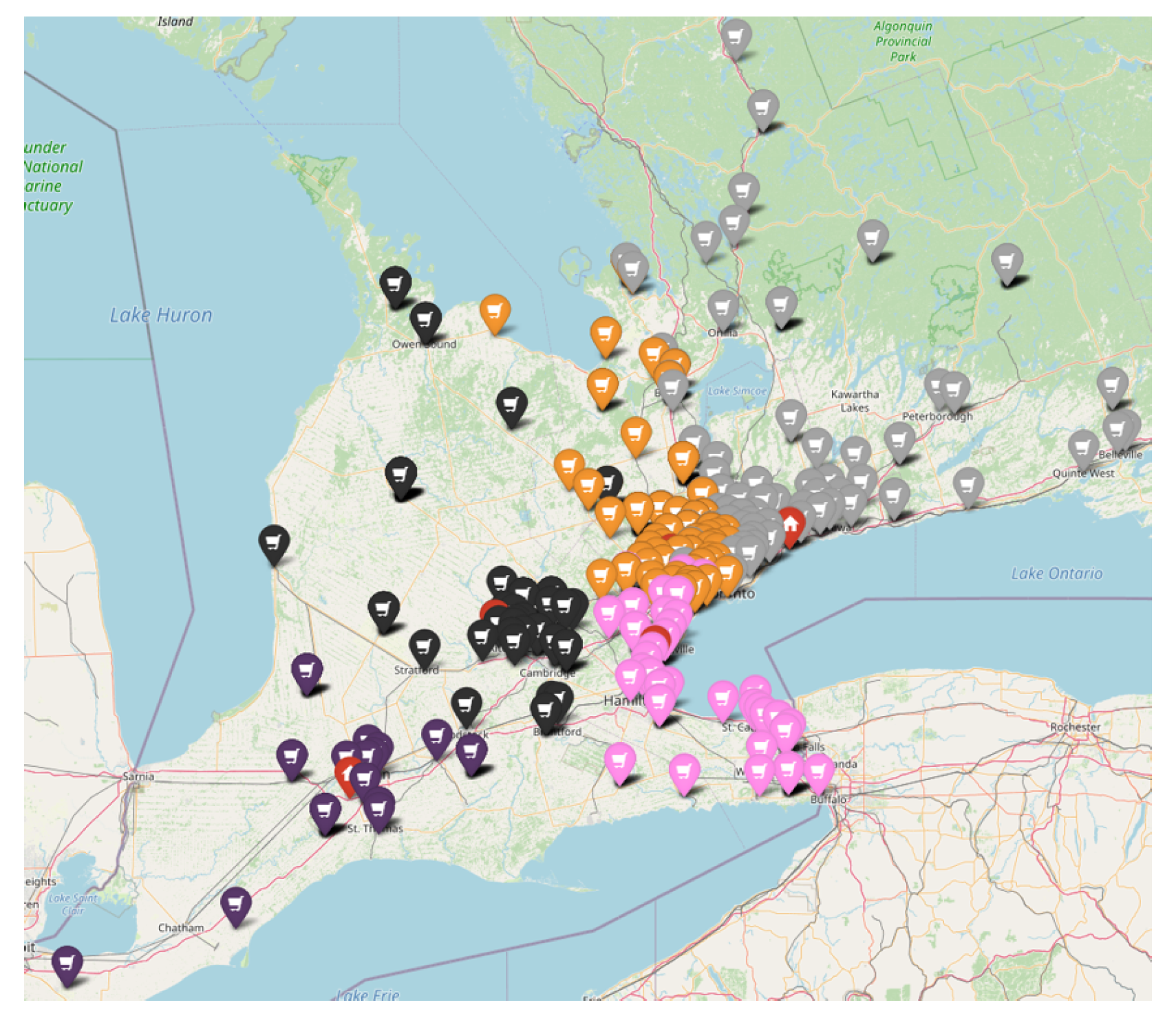
Note, in Figure 1, what happens in a solution of the model, for example, with τ = 0.1 . With this tight parameter value, Equations (4)–(6) limit the unbalance value, forcing the number of opportunities for commercial teams to be very close to the ideal balanced number of opportunities, which is the average number of opportunities multiplied by the number of workers in the team ( τ = 0.1 means a maximum deviation of 10 % from the ideal). In consequence, the total distance in the sectors (Equation (1)) is high. If the value of τ is increased, it can be seen in Figure 1 that other optimal solutions are achieved with worse balance between the teams, letting the number of opportunities in each team deviate more from the ideal but positively impacting the compactness of the sectors, achieving less total distance. Although all solutions for the multiple values of τ have been analyzed by the company, we only show here, as an example, the comparison between two solutions that favor opposing goals: τ = 0.2 for a more balanced but less compact solution and τ = 0.8 for a less balanced but more compact solution.
The compactness criterion was shown by plotting the clients in a map (Figure 2 and Figure 3), where each group color corresponds to a commercial teams’ assignment and each commercial team is represented in bright red.
The balance criterion is shown in Table 2, where the balance value is visible ( v V n v × x c v ( μ l + μ m + μ h ) × s c ), as well as the total opportunities and number of workers in each commercial team. Note that, for a better value of balance, the value in the ‘Balance’ column should be as close to 1 as possible. The solutions with lower values of τ are more balanced and less compact than the solutions with a higher value of this parameter. For example, the solution for branch A considering τ = 0.2 has balance value 1.03 , which is very close to 1, and it is more balanced than the solution obtained considering τ = 0.8 , which has a balance value of 0.83 (not so close to 1). A low value in the model parameter τ ensures fairness and equal opportunities between workers. A high value in the parameter τ allows the team to have a number of opportunities further away from the expected value per worker, which means that some workers will have fewer sales opportunities and other workers will have more. Increasing τ produces more compact sectors but causes a larger variance in the amount of workload per worker and greater discrepancies between workers. Also note that branches with three workers are naturally assigned a larger number of sales opportunities than branches with just one worker.
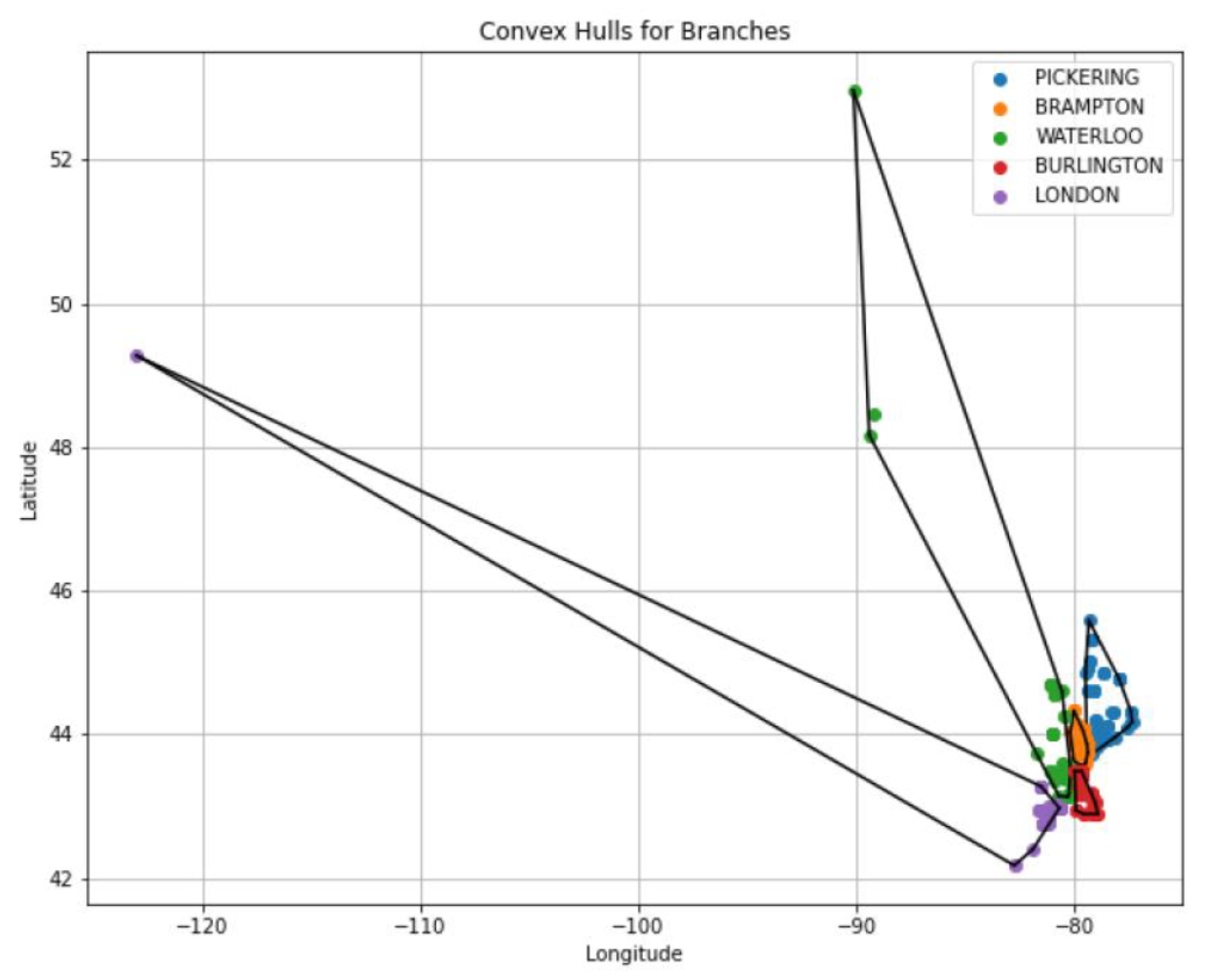
However, given the need to establish clearly defined geographic sectors, this initial solution could not be accepted as final, since sectors overlapped and there were cases of territories assigned to a team that comprised clients of another team. This is a problem to implement in practice and makes it difficult to assign a team when a new client appears. Therefore, the convex hulls of the set of points that form each sector were built and the assignments that led to potential overlaps between sectors were removed. This made it possible to define non-overlapping convex polygons representing distinct geographic areas. These results can be easily visualized in Figure 4, where each point corresponds to the geographic coordinates of a customer and the color represents the respective sales team.
As for the remaining clients whose assignments were removed (and therefore are not represented in Figure 4), they were reassigned to sales teams based on the following criteria:
  • If a client falls within one of the previously defined convex polygons, they are assigned to the sales team associated with that polygon;
  • Otherwise, the two shortest distances to the existing convex polygons are considered, and the client is assigned to the polygon whose corresponding sales team has the lowest ‘Balance’ value.
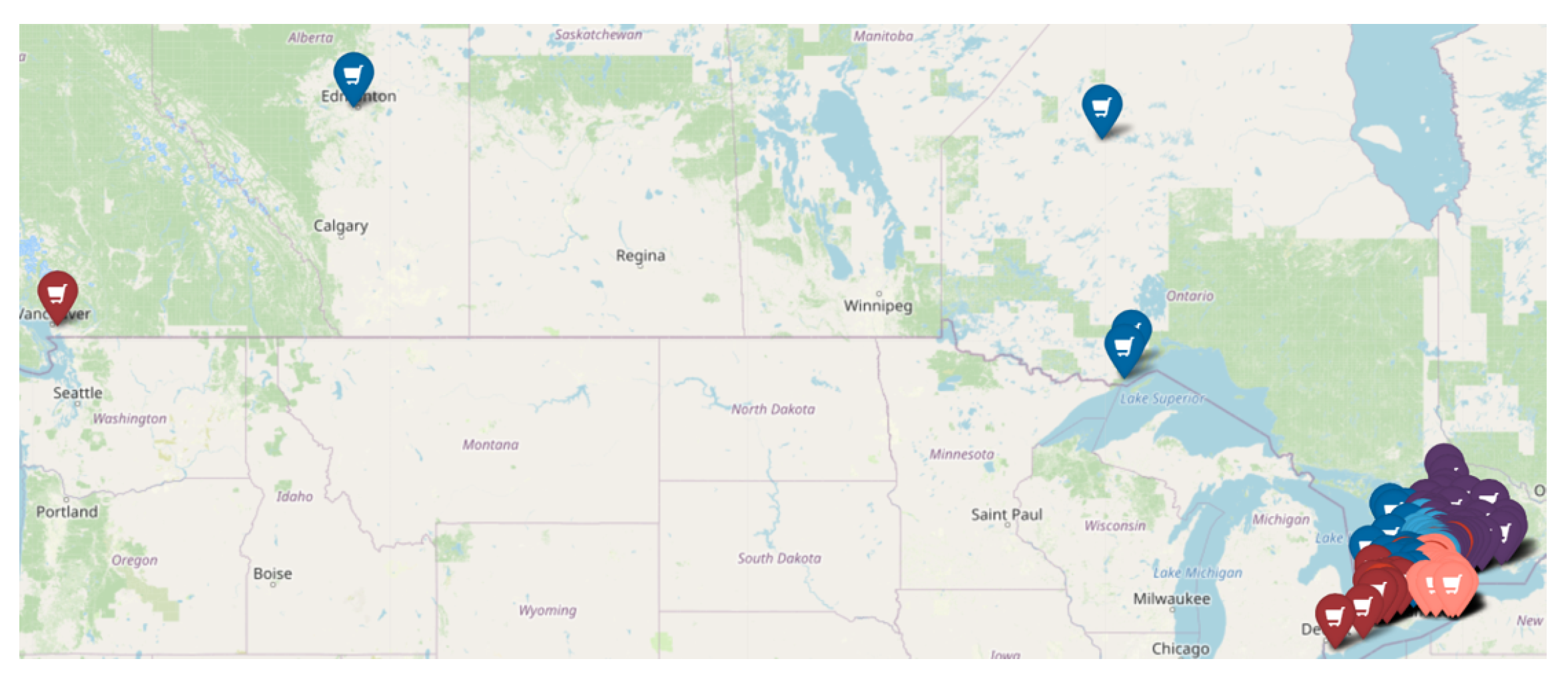
The results are shown in Figure 5 and Figure 6, where it can be observed that the sectors no longer overlap, as was the case in Figure 2 and Figure 3. To assess the model’s impact and effectiveness, we compared its results with the sectorization that the company currently has. While the current company sectorization has an unbalance value of 3.42 in total, the final proposed sectorization achieves a total unbalance value of 2.72, distributing more evenly the 2142 opportunities between the 10 workers. This means an improvement of 20.55 % in balance. The new proposed solution also affected the compactness of the sectors, improving the total distance by 18.36 % .
This final sectorization was well received by the company and its commercial teams, as it corresponded to an effort for minimizing traveling and achieving equal sales opportunities between teams for the three types of customers.
This model was developed, simulated, optimized, and fully implemented in a real industrial environment. The implementation of the model via the Python language and Power BI works in such a way that new data/clients may be enclosed in the process, and parametrization may be easily modified to encompass possible management decisions (e.g., the tolerance or the number of commercial teams may be settled in the front-end) in a very user-friendly way. The data-cleaning pipeline was also automated to allow an end-user without profound mathematical knowledge (as the majority of commercial team leaders are) to retrieve new and suitable solutions for the business. As a consequence and in order to achieve the main goal of this work, that is, to tackle a real industrial problem and to provide updated solutions to the company data changes that occur almost continuously, some simplifications were made. For example, the distance matrix and transportation costs are estimated, instead of accurately calculated. It is also important to state that the key parameters of the model (such as weights in AHP, capacity limits, or transportation costs) were defined by the company according to the knowledge of the business managers. For future work, ways for increasing the accuracy of the simplifications referred to in the previous paragraph, as well as to access the exactness of the key model parameters defined by the company, are to be performed.

5. Discussion: Could ChatGPT Accomplish This, Instead of a Mathematician?

In recent years, artificial intelligence (AI) has shown itself increasingly capable of performing a wide range of tasks previously associated exclusively with humans. The rise of large language models (LLMs), such as ChatGPT, highlights this ability across various areas. AI is steadily entering the management, work, and organizational ecosystems, with AI-based applications assisting employees with daily tasks, project management, and decision-making [43]. Traditional AI recognizes patterns and optimizes classification and decision-making, but ChatGPT can ‘hallucinate’ and generate output indistinguishable from human work [44]. While the adoption of traditional AI has been found to positively affect the revenue growth of European SMEs [45], the successful adoption of AI is a complex and multifaceted process that requires careful consideration of various factors [43].
The ultimate goal of this study is to determine whether ChatGPT can replace a mathematician, i.e., if it can achieve the same result as a mathematician given the same initial information.
After the mathematician solved the challenge proposed by this company with success, an experiment was made, prompting ChatGPT with the information and requirements provided initially by the company to the mathematician. Would ChatGPT solve this problem well?

5.1. Input

Firstly, the context and goal of the project was given as input to ChatGPT:
  • Context: The Canadian market holds enormous potential, making the commercial teams of the company in question play a crucial role. However, evaluating commercial performance is challenging—currently, only revenue is considered, which is a poor approach. Given the geographical size of Canada, a review of geographical assignments by commercial team may be justified (the decision may come from the outputs of the previous point).
  • Objective: Evaluation model of commercial teams’ performance. Optimization of geographical segments/clients assigned per commercial team.
The second input given to ChatGPT was a description of the files provided:
-
Excel file containing data related to sales of parts and equipment from 1 January 2018, to 30 September 2023. Existing columns: ‘Commercial Team’ (name of the commercial team), ‘Region’, ‘Division’, ‘Billing Date’, ‘Sale Type’, ‘Price’ (selling price), ‘Profit’, ‘Customer Number’, ‘Article Group’ (group of the sold article), and ‘Article Code’ (code of the sold article).
-
Excel file containing data related to opportunities for parts and equipment from 2018 to 2023. Existing columns: ‘Commercial Team’ (name of the commercial team), ‘Region’, ‘Division’, ‘Closing Date’ (date when the opportunity was closed or is expected to close), ‘Price’ (selling price), ‘Customer Number’, ‘Status’ (status of the opportunity), and ‘Evaluation’ (evaluation of the opportunity).
-
Excel file containing data related to services (e.g., equipment repair) provided by the company from 1 January 2018, to 27 November 2023. Existing columns: ‘Commercial Team’ (name of the commercial team), ‘Region’, ‘Division’, ‘Billing Date’, ‘Price’ (service cost), and ‘Customer Number’.
-
Excel file containing data related to the organization of commercial teams in the year 2023. Existing columns: ‘Commercial Team’ (name of the commercial team), ‘Name’ (worker’s name), ‘Region’, ‘Division’, and ‘Title’ (worker’s position).
-
Excel file containing data related to the addresses of commercial teams. Existing columns: ‘Commercial Team’ (name of the commercial team) and ‘Postal Code’ (postal code corresponding to the location of the commercial team).
-
Excel file containing data related to the addresses of customers who have made a purchase or received a service from the company. Existing columns: ‘Customer Number’, ‘Province’, and ‘Postal Code’ (province and postal code corresponding to the location of the customer).

5.2. Output

The output given by ChatGPT was a Python code which performed the following:
  • The code imports necessary libraries such as pandas for data manipulation, numpy for numerical computations, train_test_split for splitting data into training and testing sets, RandomForestRegressor for building a regression model, mean_squared_error for evaluating model performance, and matplotlib.pyplot for data visualization.
  • Excel files containing sales, opportunities, services, team organization, and customer address data are loaded into pandas’ DataFrames.
  • Data from different sources (sales, opportunities, services) are concatenated into a single DataFrame. Data from the year 2023 are filtered, and team data from 2023 are merged with the filtered data based on the ’Commercial Team’ column.
  • Performance metrics such as Total Sales, Average Sales, Total Profit, Number of Unique Customers, and Number of Transactions are calculated for each commercial team using groupby and aggregation functions.
  • The column names of the performance metrics’ DataFrames are renamed for easier interpretation.
  • A custom metric (‘Custom Metric’) is added to the performance metrics’ DataFrames to illustrate a fictitious metric. It is calculated by dividing total sales by the number of unique customers.
  • Features (X) and target variable (y) are defined. The data is split into training and testing sets. A Random Forest Regressor model is instantiated and trained on the training data.
  • The trained model is used to make predictions on the testing data, and mean squared error (MSE) is calculated to evaluate the model’s performance.
  • The importance of features in the trained model is visualized using a bar plot.
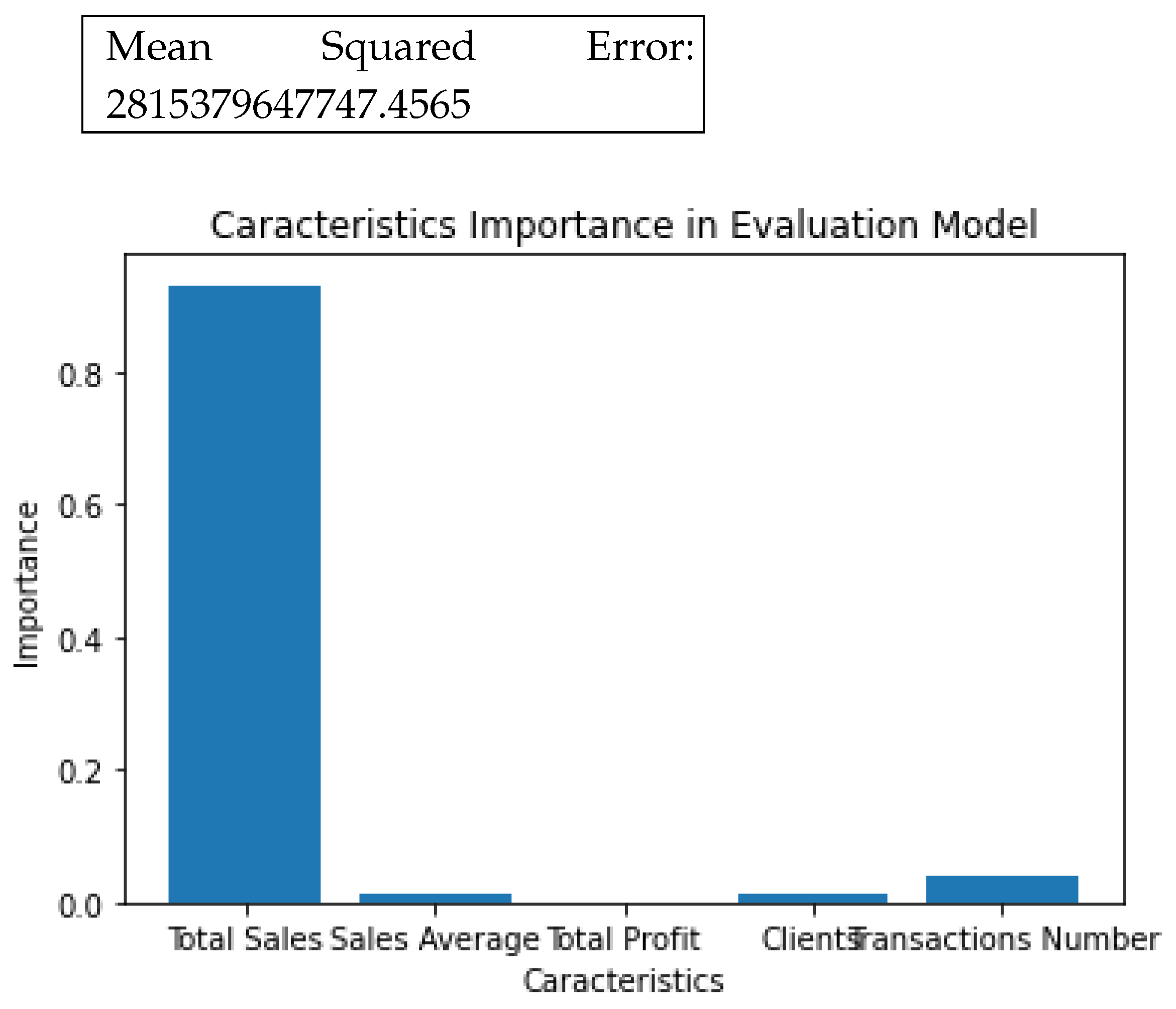
After replacing the correct directory for each file, the code was executed without errors and the outputs in Figure 7 were obtained.
It was observed that ChatGPT creates a model that uses the provided features (Total Sales, Average Sales, Total Profit, Unique Customers, and Number of Transactions) to predict the customized performance metric of commercial teams. Then, it provides the relative importance of each feature in the model, aiming to understand which features have the most impact on the customized metric.

5.3. Problems of ChatGPT’s Approach

The first immediately visible issue is that ChatGPT did not even address the sectorization problem.
Regarding the rest of the approach, it appears to be unsatisfactory, as it overlooks several aspects of the provided dataset. For example, only the sales file has a column related to profit.
The conclusion presented in the output provided by ChatGPT would imply that it is only worthwhile to evaluate the performance of commercial teams based on Total Sales, which would be extremely incomplete for the business.
It is worth noting that this result does not solve the project at hand at all, nor does it come close to producing a presentable solution.
There are some lessons learned from the attempt to use ChatGPT for solving this mathematical optimization problem. While useful for building intuition and providing a general outline, ChatGPT has limits when applied to advanced mathematical optimization. The tool cannot fully replace specialized methods or expert knowledge in this domain. It has value as a starting point, but not as a replacement for deep mathematical reasoning. Solving mathematical optimization problems with rigor requires precise problem statements, guided prompting for detailed steps, and critical validation of AI-generated solutions to ensure correctness and applicability. Overall, the exercise showed that ChatGPT can serve as a useful starting point for framing and exploring optimization problems, but achieving depth requires precise problem formulation, structured guidance, and critical human oversight.

6. Conclusions

In conclusion, this study has addressed the challenge of sectorization in a large company in Canada, by employing advanced optimization techniques and the RFM model. Through this analysis, a linear integer programming model was formulated, which was solved using the pyscipopt package in Python. By integrating the RFM results into the sectorization model, equitable sales potential was ensured between teams by balancing opportunities based on the value of each client.
This study reveals that the formulated sectorization plan presents significant solutions that can be chosen based on the importance given to compactness and balance, being flexible to the company’s preferences.
Furthermore, it contributes to the understanding of sectorization problems and demonstrates the effectiveness of using advanced optimization techniques and data-driven models to address such challenges. This approach provides valuable observations for companies seeking to optimize their commercial teams’ performance and resource allocation strategies.
With the preliminary exploratory exercise that was made, comparing the human solution to this business problem and the ChatGPT solution, it can also come to the conclusion that, although ChatGPT is effective at performing specific and routine tasks, its ability to develop complex projects, particularly in fields like advanced mathematics, is still far from surpassing human capability. Artificial intelligence is valuable for automating simple processes and providing quick solutions, but its lack of deep understanding, intuition, and creativity limits its ability to address abstract and innovative mathematical challenges.
The crucial role of a mathematician, with their capacity for abstract reasoning, mathematical intuition, and conceptual understanding, remains unparalleled, highlighting that artificial intelligence is unable to replace the unique and indispensable contribution of human professionals in this specific field.

Author Contributions

Conceptualization, A.M.C., M.C., F.V. and P.L.; methodology, A.M.C. and C.L.; software, A.M.C., F.V. and P.L.; validation, F.V. and P.L.; formal analysis, C.L., M.C., J.S. and S.R.; investigation, A.M.C., C.L., M.C., J.S. and S.R.; resources, A.M.C., F.V. and P.L.; data curation, A.M.C., F.V. and P.L.; writing—original draft preparation, A.M.C.; writing—review and editing, C.L., M.C., J.S. and S.R.; visualization, A.M.C.; supervision, C.L., F.V. and P.L.; project administration, M.C. and P.L.; funding acquisition, M.C. and P.L. All authors have read and agreed to the published version of the manuscript.

Funding

This research received no external funding.

Data Availability Statement

Data is unavailable due to privacy restrictions.

Conflicts of Interest

Ana Miguel Carvalho, Filipa Vieira and Pedro Louro were employed by Nors. Ana Miguel Carvalho was employed by BPI. The remaining authors declare that the research was conducted in the absence of any commercial or financial relationships that could be construed as a potential conflict of interest.

References

  1. Zuse Institute Berlin. SCIP—Solving Constraint Integer Programs. 2025. Available online: https://www.scipopt.org/ (accessed on 13 May 2024).
  2. Achterberg, T. SCIP: Solving constraint integer programs. Math. Program. Comput. 2009, 1, 1–41. [Google Scholar] [CrossRef]
  3. Patron, M. Case Study: Applying RFM segmentation to the SilverMinds catalogue. J. Direct Data Digit. Mark. Pr. 2004, 5, 269–275. [Google Scholar] [CrossRef]
  4. Wei, J.-T.; Lin, S.-Y.; Wu, H.-H. A review of the application of RFM model. Afr. J. Bus. Manag. 2010, 4, 4199–4206. [Google Scholar]
  5. Blattberg, R.C.; Kim, B.D.; Neslin, S.A. RFM Analysis. In Database Marketing: Analyzing and Managing Customers; Springer: New York, NY, USA, 2008; pp. 323–337. [Google Scholar] [CrossRef]
  6. Herrera-Viedma, E.; Carrasco, R.A.; Blasco, M.F.; García-Madariaga, J. A Fuzzy Linguistic RFM Model Applied to Campaign Management. Int. J. Interact. Multimed. Artif. Intell. 2019, 5, 21–27. [Google Scholar] [CrossRef]
  7. Colombo, R.; Jiang, W. A stochastic RFM model. J. Interact. Mark. 1999, 13, 2–12. [Google Scholar] [CrossRef]
  8. Zong, Y.; Xing, H. Customer stratification theory and value evaluation—Analysis based on improved RFM model. J. Intell. Fuzzy Syst. 2021, 40, 4155–4167. [Google Scholar] [CrossRef]
  9. Heldt, R.; Silveira, C.S.; Luce, F.B. Predicting customer value per product: From RFM to RFM/P. J. Bus. Res. 2021, 127, 444–453. [Google Scholar] [CrossRef]
  10. Martínez, R.G.; Carrasco, R.A.; Sanchez-Figueroa, C.; Gavilan, D. An RFM Model Customizable to Product Catalogues and Marketing Criteria Using Fuzzy Linguistic Models: Case Study of a Retail Business. Mathematics 2021, 9, 1836. [Google Scholar] [CrossRef]
  11. Ernawati, E.; Baharin, S.S.K.; Kasmin, F. A review of data mining methods in RFM-based customer segmentation. In Proceedings of the 2nd Annual Conference of Science and Technology (ANCOSET 2020), Malang, Indonesia, 28 November 2020; Journal of Physics: Conference Series. IOP Publishing: Bristol, UK, 2021; Volume 1869. [Google Scholar] [CrossRef]
  12. Wu, J.; Shi, L.; Yang, L.; Niu, X.; Li, Y.; Cui, X.; Tsai, S.B.; Zhang, Y. User Value Identification Based on Improved RFM Model and K-Means++ Algorithm for Complex Data Analysis. Wirel. Commun. Mob. Comput. 2021, 2021, 9982484. [Google Scholar] [CrossRef]
  13. Rungruang, C.; Riyapan, P.; Intarasit, A.; Chuarkham, K.; Muangprathub, J. RFM model customer segmentation based on hierarchical approach using FCA. Expert Syst. Appl. 2024, 237, 121449. [Google Scholar] [CrossRef]
  14. Robert, C.B.; Byung, D.K.; Scott, A.N. Database Marketing: Analyzing and Managing Customers; Springer: Berlin/Heidelberg, Germany, 2008. [Google Scholar]
  15. Christy, A.J.; Umamakeswari, A.; Priyatharsini, L.; Neyaa, A. RFM ranking—An effective approach to customer segmentation. J. King Saud Univ.-Comput. Inf. Sci. 2021, 33, 1251–1257. [Google Scholar] [CrossRef]
  16. Hsu, P.Y.; Huang, C.W. IECT: A methodology for identifying critical products using purchase transactions. Appl. Soft Comput. 2020, 94, 106420. [Google Scholar] [CrossRef]
  17. Koch, R. The 80/20 Principle: The Secret of Achieving More with Less: Updated 20th Anniversary Edition of the Productivity and Business Classic; Hachette UK: London, UK, 2011. [Google Scholar]
  18. Gomes, M.A.; Meisen, T. A review on customer segmentation methods for personalized customer targeting in e-commerce use cases. Inf. Syst. e-Bus. Manag. 2023, 21, 527–570. [Google Scholar] [CrossRef]
  19. Handojo, A.; Pujawan, N.; Santosa, B.; Singgih, M.L. A multi layer recency frequency monetary method for customer priority segmentation in online transaction. Cogent Eng. 2023, 10, 2162679. [Google Scholar] [CrossRef]
  20. Lopes, C.; Rodrigues, A.M.; Romanciuc, V.; Ferreira, J.S.; Öztürk, E.G.; Oliveira, C. Divide and Conquer: A Location-Allocation Approach to Sectorization. Mathematics 2023, 11, 2553. [Google Scholar] [CrossRef]
  21. Kalcsics, J.; Ríos-Mercado, R.Z. Districting Problems. In Location Science; Laporte, G., Nickel, S., Saldanha da Gama, F., Eds.; Springer International Publishing: Cham, Switzerland, 2019; pp. 705–743. [Google Scholar] [CrossRef]
  22. Zoltners, A.A.; Sinha, P. The 2004 ISMS Practice Prize Winner—Sales Territory Design: Thirty Years of Modeling and Implementation. Mark. Sci. 2005, 24, 313–331. [Google Scholar] [CrossRef]
  23. Darmian, S.M.; Fattahi, M.; Keyvanshokooh, E. An optimization-based approach for the healthcare districting under uncertainty. Comput. Oper. Res. 2021, 135, 105425. [Google Scholar] [CrossRef]
  24. Tavares-Pereira, F.; Figueira, J.R.; Mousseau, V.; Roy, B. Multiple criteria districting problems: The public transportation network pricing system of the Paris region. Ann. Oper. Res. 2007, 154, 69–92. [Google Scholar] [CrossRef]
  25. Camacho-Collados, M.; Liberatore, F.; Angulo, J.M. A multi-criteria police districting problem for the efficient and effective design of patrol sector. Eur. J. Oper. Res. 2015, 246, 674–684. [Google Scholar] [CrossRef]
  26. Bouzarth, E.L.; Forrester, R.; Hutson, K.R.; Reddoch, L. Assigning students to schools to minimize both transportation costs and socioeconomic variation between schools. Socio-Econ. Plan. Sci. 2018, 64, 1–8. [Google Scholar] [CrossRef]
  27. Shanker, R.J.; Turner, R.E.; Zoltners, A.A. Sales territory design: An integrated approach. Manag. Sci. 1975, 22, 309–320. [Google Scholar] [CrossRef]
  28. Sandoval, M.G.; Álvarez-Miranda, E.; Pereira, J.; Ríos-Mercado, R.Z.; Díaz, J.A. A novel districting design approach for on-time last-mile delivery: An application on an express postal company. Omega 2022, 113, 102687. [Google Scholar] [CrossRef]
  29. Álvarez-Miranda, E.; Pereira, J. A districting application with a quality of service objective. Mathematics 2021, 10, 13. [Google Scholar] [CrossRef]
  30. Corley, H., Jr.; Roberts, S. A partitioning problem with applications in regional design. Oper. Res. 1972, 20, 1010–1019. [Google Scholar] [CrossRef]
  31. Martinho, A.; Alves, E.; Rodrigues, A.M.; Ferreira, J.S. Multicriteria location-routing problems with sectorization. In Proceedings of the Operational Research: IO2017, Valença, Portugal, 28–30 June 2018; Springer: Berlin/Heidelberg, Germany, 2018; pp. 215–234. [Google Scholar]
  32. Hewitt, M.; Frejinger, E. Data-driven optimization model customization. Eur. J. Oper. Res. 2020, 287, 438–451. [Google Scholar] [CrossRef]
  33. Kalcsics, J.; Nickel, S.; Schröder, M. Towards a unified territorial design approach—Applications, algorithms and GIS integration. Top 2005, 13, 1–56. [Google Scholar] [CrossRef]
  34. Ríos-Mercado, R.Z.; López-Pérez, J.F. Commercial territory design planning with realignment and disjoint assignment requirements. Omega 2013, 41, 525–535. [Google Scholar] [CrossRef]
  35. Saaty, T.L. The Analytic Hierarchy Process in Conflict Management. Int. J. Confl. Manag. 1990, 1, 47–68. [Google Scholar] [CrossRef]
  36. Albayrak, E.; Erensal, Y. Using analytic hierarchy process (AHP) to improve human performance: An application of multiple criteria decision making problem. J. Intell. Manuf. 2004, 15, 491–503. [Google Scholar] [CrossRef]
  37. Baskir, M.B. A novel belief-based QFD-AHP model in interval type-2 fuzzy environment for lean after-sales service in automotive industry. Int. J. Lean Six Sigma 2023, 14, 653–678. [Google Scholar] [CrossRef]
  38. Ben Ali, M.; Rauch, E. Sustainable Mobility Transition: A SWOT-AHP Analysis of the Case Study of Italy. Sustainability 2024, 16, 4861. [Google Scholar] [CrossRef]
  39. James, A.T.; Asjad, M.; Panchal, R. Purchase decision making of garage equipment using an integrated fuzzy AHP and grey relation analysis method. Grey Syst. Theory Appl. 2022, 13, 238–260. [Google Scholar] [CrossRef]
  40. Paredes Rodríguez, A.M.; Bravo Bastidas, J.J.; Osorio Gómez, J.C.; Peña Orozco, D.L.; González Feliu, J. Fuzzy AHP TOPSIS Methodology for Multicriteria ABC Inventory Classification. J. Eng. 2023, 2023, 7661628. [Google Scholar] [CrossRef]
  41. Ortiz-Barrios, M.; Borrego-Areyanes, A.A.; Gómez-Villar, I.D.; De Felice, F.; Petrillo, A.; Gul, M.; Yucesan, M. A multiple criteria decision-making approach for increasing the preparedness level of sales departments against COVID-19 and future pandemics: A real-world case. Int. J. Disaster Risk Reduct. 2021, 62, 102411. [Google Scholar] [CrossRef]
  42. Pant, S.; Kumar, A.; Ram, M.; Klochkov, Y.; Sharma, H.K. Consistency Indices in Analytic Hierarchy Process: A Review. Mathematics 2022, 10, 1206. [Google Scholar] [CrossRef]
  43. Tursunbayeva, A.; Chalutz-Ben Gal, H. Adoption of artificial intelligence: A TOP framework-based checklist for digital leaders. Bus. Horizons 2024, 67, 357–368. [Google Scholar] [CrossRef]
  44. Retkowsky, J.; Hafermalz, E.; Huysman, M. Managing a ChatGPT-empowered workforce: Understanding its affordances and side effects. Bus. Horizons 2024, 67, 511–523. [Google Scholar] [CrossRef]
  45. Ardito, L.; Filieri, R.; Raguseo, E.; Vitari, C. Artificial intelligence adoption and revenue growth in European SMEs: Synergies with IoT and big data analytics. Internet Res. 2024. [Google Scholar] [CrossRef]
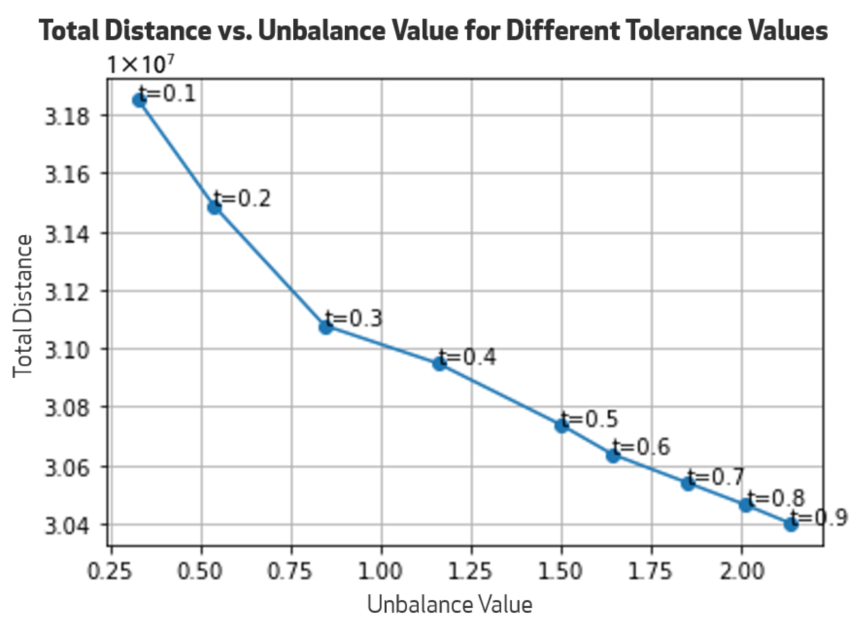
Figure 1. Pareto front.
Mathematics 13 02940 g001
Figure 2. Sectorization for τ = 0.2 (zoomed in on the Toronto region).
Mathematics 13 02940 g002
Figure 3. Sectorization for τ = 0.8 (zoomed in on the Toronto region).
Mathematics 13 02940 g003
Figure 4. Convex polygons after eliminating possible overlaps in assignments.
Mathematics 13 02940 g004
Figure 5. Final sectorization.
Mathematics 13 02940 g005
Figure 6. Final sectorization (zoomed in).
Mathematics 13 02940 g006
Figure 7. ChatGPToutput.
Mathematics 13 02940 g007
Table 1. Sets and parameters of the model.
SetsDescription
LSet of Low-Value customers
MSet of Mid-Value customers
HSet of High-Value customers
V = L M H Set of basic units (customers)
CSet of sectors or territories (commercial teams)
ParametersDescription
d c v Distance from commercial team c to customer v
n v Measure of the number of opportunities relative to customer v
s c Measure of the number of workers in commercial team c
μ l Average number of opportunities, relative to Low-Value customers, per worker
μ m Average number of opportunities, relative to Mid-Value customers, per worker
μ h Average number of opportunities, relative to High-Value customers, per worker
τ Tolerance
kNumber of commercial teams, k = | C |
Table 2. Number of opportunities for each commercial team.
BranchNumber of WorkersTotal OpportunitiesBalance τ
A36631.030.2
5360.830.8
B25121.200.2
7681.790.8
C35630.880.2
4130.640.8
D12271.060.2
2871.340.8
E11770.830.2
1380.640.8
Disclaimer/Publisher’s Note: The statements, opinions and data contained in all publications are solely those of the individual author(s) and contributor(s) and not of MDPI and/or the editor(s). MDPI and/or the editor(s) disclaim responsibility for any injury to people or property resulting from any ideas, methods, instructions or products referred to in the content.