Computing One-Bit Compressive Sensing via Alternating Proximal Algorithm

Abstract

It is challenging to recover a real sparse signal using one-bit compressive sensing. Existing methods work well when there is no noise (sign flips) in the measurements or the noise level or a priori information about signal sparsity is known. However, the noise level and a priori information about signal sparsity are not always known in practice. In this paper, we propose a robust model with a non-smooth and non-convex objective function. In this model, the noise factor is considered without knowing the noise level or a priori information about the signal sparsity. We develop an alternating proximal algorithm and prove that the sequence generated from the algorithm converges to a local minimizer of the model. Our algrithm possesses high time efficiency and recovery accuracy. It performs better than other algorithms tested in our experiments when the the noise level and the sparsity of the signal is known.

1. Introduction

One-bit compressive sensing (CS) was originally introduced in [1]. It has been applied extensively, such as in [2,3,4,5]. Let x be a sparse signal in ${\mathcal{R}}^n$ and B be an $m\times n$ matrix. The measurement vector $b\in {\mathcal{R}}^m$ of the signal x is calculated via

$$b=\mathcal{A}x=\mathrm{sign}(Bx)$$

(1)

where $\mathrm{sign}(·)$ operates componentwise with $\mathrm{sign}(z)=1$ if $z\ge 0$ and $\mathrm{sign}(z)=-1$ otherwise. The measurement operator $\mathcal{A}:{\mathcal{R}}^n\to {\{-1,1\}}^m$ is called the one-bit scalar quantizer. The prime target of one-bit CS is to recover the sparse signal x from the one-bit observation b and the measurement matrix B. We will now review existing models for the one-bit CS problem. The ideal optimization model is the following $l_0$-norm minimization:

$$\underset{x\in {\mathcal{R}}^n}{min}\{{\parallel x\parallel }_0\},\mathrm{s}.\mathrm{t}.b=\mathrm{sign}(Bx),$$

(2)

where ${\parallel x\parallel }_0$ is the $l_0$-norm of x, counting the number of its non-zero entries. The NP-hardness of model (2) makes approximation challenging. The earliest attempt can be traced back to [1], in which the ideal model (2) was relaxed by

$$\underset{x\in {\mathcal{R}}^n}{min}\{{\parallel x\parallel }_1\},\mathrm{s}.\mathrm{t}.YBx\ge 0,\parallel x\parallel =1,$$

(3)

where Y is a diagonal matrix with diagonal entries from b, and ${\parallel x\parallel }_1$ is the sum of the absolute values of the components of x. This model is valid for the noiseless case. For the case in which the measurement $Bx$ is contaminated by noise (sign flips), instead of solving model (3), ref. [1] relaxed it as follows:

$$\underset{x\in {\mathcal{R}}^n}{min}\{{\parallel x\parallel }_1+\lambda {{\parallel [YBx]}_{-}\parallel }^2\},\mathrm{s}.\mathrm{t}.\parallel x\parallel =1,$$

(4)

where $\lambda >0$ is a parameter, and ${[·]}_{-}$ represents the operator projected onto the convex set $\{u:u\in {\mathcal{R}}^m\mathrm{and}{u}_i\le 0,i=1,2,\cdots ,m\}$. Since both models (3) and (4) minimize convex objective functions over the non-convex unit sphere, to overcome difficulties resulting from non-convexity, the following model was proposed in [6]:

$$\underset{x\in {\mathcal{R}}^n}{min}{\{\parallel x\parallel }_1{\},\mathrm{s}.\mathrm{t}.YBx\ge 0,\parallel Bx\parallel }_1=r,$$

(5)

where r is an arbitrary positive number. Obviously, the set determined by the two constraints is convex. In addition, the model can be efficiently solved using a linear programming method. However, it was shown numerically that solutions of model (5) are not sparse enough when the signal $x\in {\mathcal{R}}^n$ is known to have s-sparsity, that is, $x\in \{x\in {\mathcal{R}}^n|{\parallel x\parallel }_0\le s\}.$ A newer model for the one-bit CS model,

$$\underset{x\in {\mathcal{R}}^n}{min}\{h({[YBx]}_{-})\}{,\mathrm{s}.\mathrm{t}.\parallel x\parallel }_0\le s,\parallel x\parallel =1$$

(6)

was proposed in [7], where function h is either ${\parallel ·\parallel }_1$ or ${\parallel ·\parallel }^2$. An algorithm called binary iterative hard thresholding (BIHT) was developed for solving model (6). Based on BIHT, the adaptive outlier pursuit (AOP) technique was introduced in [8] for solving the following one-bit CS model:

$$\underset{x\in {\mathcal{R}}^n}{min}\{h({[\mathsf{\Lambda }YBx]}_{-})\},\mathrm{s}.\mathrm{t}.\sum _{i=1}^m(1-{\mathsf{\Lambda }}_{ii})\le {L,\parallel x\parallel }_0\le s,\parallel x\parallel =1,$$

(7)

where L is the noise level, that is, there are at most L measurements in y that are wrongly detected (with sign flips), and $\mathsf{\Lambda }$ is an $m\times m$ diagonal matrix whose diagonal entries are either 1 or 0. If ${\mathsf{\Lambda }}_{ii}=1$, then the ith component $y_i$ of y is correct; otherwise, it is incorrect. If the matrix $\mathsf{\Lambda }$ is specified, model (7) can be reduced to model (6) by disregarding the incorrect measurements. However, in model (7), the noise level L must be given in advance, a condition that is hardly ever satisfied in practice. The following one-sided $l_0$(OSL0) model was proposed in [9] for when L is unavailable:

$$\underset{x\in {\mathcal{R}}^n,v\in {\mathcal{R}}^m}{min}{\{\lambda \parallel [v-ϵe]}_{-}{\parallel }_0+{\displaystyle \frac{\gamma }{2}}{\parallel YBx-v\parallel }^2+{\displaystyle \frac{\beta }{2}}{\parallel x\parallel }^2{\},\mathrm{s}.\mathrm{t}.\parallel x\parallel }_0\le s,$$

(8)

where $ϵ$, $\lambda$, $\gamma$ and $\beta$ are positive parameters, and e denotes the vector in ${\mathcal{R}}^m$ with all components equal to one. In [9], a fixed-point proximity algorithm was proposed for solving model (8). It was shown that the sequence generated from the fixed-point proximity algorithm converges to a local minimizer of the objective function of model (8) and converges to a global minimizer of the function as long as the initial estimate is sufficiently close to any global minimizer of the function. In [10], the authors took advantage of $l_1$-regularized least squares to address the one-bit CS problem regardless of the sign information of $Bx$, namely,

$$\underset{x\in {\mathcal{R}}^n}{min}{\{\parallel x\parallel }_1{+\lambda \parallel b-Bx\parallel }^2\},$$

(9)

where $\lambda$ is a given positive parameter. A primal dual active set algorithm was proposed to solve model (9) and proved to converge within one step under two assumptions: the submatrix of B indexed on the nonzero components of the sparse solution is full row rank and the initial point is sufficiently close to the sparse solution. Therefore, the generated sequence again has a local convergence property. To eliminate the assumptions on data B for better convergence results, xiu et al. [11] proposed the following double-sparsity constrained model:

$$\underset{x\in {\mathcal{R}}^n,y\in {\mathcal{R}}^m}{min}{\{\parallel YBx+y-ϵe\parallel }^2+{\eta \parallel x\parallel }^2{\},\mathrm{s}.\mathrm{t}.\parallel x\parallel }_0\le s,{\parallel y_{+}\parallel }_0\le k,$$

(10)

where $\parallel y_{+}{\parallel }_0={\parallel {[-y]}_{-}\parallel }_0$, $\eta >0$ is a penalty parameter and $s\ll n$ and $k\ll m$ are two positive integers representing prior information about the upper bounds of the signal sparsity and the number of sign flips, respectively. An algorithm called Gradient projection subspace pursuit was proposed in [11] to solve model (10).

To solve the previous model, either a priori knowledge is required or the algorithm lacks convergence analysis, excluding it from many potential applications. In this study, we introduce a model for the noisy one-bit CS problem that requires neither a priori knowledge of the signal sparsity nor a priori knowledge of the noise level of the measurements. We develop an algorithm to solve the proposed model and analyze the convergence of the proposed algorithm. Our algorithm possesses high time efficiency and recovery accuracy. Moreover, it performs better than other existing algorithms when the the noise level and the sparsity of the signal is known. To summarize, our algorithm is suitable for more many practical scenarios.

2. Elementary Facts

The Euclidean scalar product of ${\mathcal{R}}^n$ and its corresponding norm are denoted by $⟨·,·⟩$, and $\parallel ·\parallel$, respectively. For a symmetric matrix A, the maximum eigenvalue is denoted by ${\lambda }_{max}(A)$. The M-norm of the vector x is denoted by ${\parallel x\parallel }_M:=\sqrt{x^{T}Mx}$ if the matrix M is positive definite.

Definition 1 

(Rockafellar and Wets [12]). Let $f:{\mathcal{R}}^n\to \mathcal{R}\cup \{+\infty \}$ be a proper lower semicontinuous function.

(i) 

 The domain of f is defined and denoted by $\mathrm{dom}f:=\{x\in {\mathcal{R}}^n|f(x)<+\infty \}$;

(ii) 

 For each $x\in \mathrm{dom}f$, the Fréchet subdifferential of f at x, written $\widehat{\partial }f(x)$, is the set of vectors $x^{\ast }\in {\mathcal{R}}^n$ that satisfies

$$\underset{y\ne x,y\to x}{lim\; inf}{\displaystyle \frac{1}{\parallel y-x\parallel }}[f(y)-f(x)-⟨x^{\ast },y-x⟩]\ge 0.$$

(11)

If $x\notin \mathrm{dom}f$, then $\widehat{\partial }f(x)=\varphi$;

(iii) 

 The limiting-subdifferential (Mordukhovich [13]), or simply the subdifferential for short, of f at $x\in \mathrm{dom}f$, written $\partial f(x)$, is defined as follows:

$$\partial f(x):=\{x^{\ast }\in {\mathcal{R}}^n|\exists x_n\to x,f(x_n)\to f(x),x_n^{\ast }\in \widehat{\partial }f(x_n)\to x^{\ast }\}.$$

(12)

A necessary (but insufficient) condition for $x\in {\mathcal{R}}^n$ to be a minimizer of a proper lower semicontinuous function f is $0\in \partial f(x)$. For a proper lower semi-continuous function $f:{\mathcal{R}}^n\to \mathcal{R}\cup \{+\infty \}$, the proximity operator of f is defined by [14]

$${\mathrm{prox}}_f(x):=arg\underset{y\in {\mathcal{R}}^n}{min}\{f(y)+{\displaystyle \frac{1}{2}}{\parallel y-x\parallel }^2\}.$$

(13)

Clearly, for any $z\in {\mathrm{prox}}_f(x)$, by the calculus of the limiting-subdifferential, we have that $x-z\in \partial f(z)$.

3. The ${\mathit{l}}_{\mathbf{1}}$ Model

A classical approach to problem (1) is the least squares (LS) approach [15], in which the estimator is chosen to minimize the data error:

$$\underset{x\in {\mathcal{R}}^n}{min}\left\{{\parallel b-\mathrm{sign}(Bx)\parallel }^2\right\}.$$

(14)

Notice that the LS solution may have a huge norm and is thus meaningless. Regularization methods are needed to stabilize the solution. The basic concept of regularization is to replace the original problem with a “nearby” problem whose solution approximates the required solution. A popular regularization technique is Tikhonov regularization [16], in which a quadratic penalty is added to the objective function:

$$\underset{x\in {\mathcal{R}}^n}{min}\{{\displaystyle \frac{\alpha }{2}}{\parallel b-\mathrm{sign}(Bx)\parallel }^2+{\displaystyle \frac{\beta }{2}}{\parallel x\parallel }^2\}.$$

(15)

The second term in the above minimization problem is a regularization term that controls the norm of the solution. Since x is a sparse signal, $l_1$ regularization (see, e.g., [17,18]) can be used to induce sparsity in the optimal solution:

$$\underset{x\in {\mathcal{R}}^n}{min}\{{\displaystyle \frac{\alpha }{2}}{\parallel b-\mathrm{sign}(Bx)\parallel }^2+{\displaystyle \frac{\beta }{2}}{\parallel x\parallel }^2+\rho {\parallel x\parallel }_1\}.$$

(16)

Notice that for any $x\in {\mathcal{R}}^n$ and $b\in {\{-1,1\}}^m$, the following identity holds:

$${\parallel b-\mathrm{sign}(Bx)\parallel }^2=4{\parallel b-\mathrm{sign}(Bx)\parallel }_0.$$

(17)

It follows from [9] (Proposition 3.1) that the function ${\parallel b-\mathrm{sign}(Bx)\parallel }_0$ can be majorized by a lower semi-continuous function ${\parallel {[YBx-ϵe]}_{-}\parallel }_0$. We therefore substitute expression ${\parallel b-\mathrm{sign}(Bx)\parallel }^2$ in model (16) by the lower semi-continuous function ${\parallel {[YBx-ϵe]}_{-}\parallel }_0$. For notational simplicity, we set $A:=YB$ and ${\phi (·):=\parallel {[·-ϵe]}_{-}\parallel }_0$ for a fixed $ϵ>0$. As a consequence, model (16) can be recast as

$$\underset{x\in {\mathcal{R}}^n}{min}\{\lambda \phi (Ax)+{\displaystyle \frac{\beta }{2}}{\parallel x\parallel }^2+\rho {\parallel x\parallel }_1\},$$

(18)

where $\lambda =2\alpha$. The objective function of model (18) is lower semi-continuous and coercive; therefore, model (18) attains its minimum. By introducing an additional variable $y\in {\mathcal{R}}^m$, we can rewrite problem (18) as

$$\begin{array}{cc}\hfill & \underset{x\in {\mathcal{R}}^n,y\in {\mathcal{R}}^m}{min}\{\lambda \phi (y)+{\displaystyle \frac{\beta }{2}}{\parallel x\parallel }^2+\rho {\parallel x\parallel }_1\}\hfill \\ \hfill & \mathrm{s}.\mathrm{t}.Ax=y.\hfill \end{array}$$

(19)

Furthermore, model (19) can be approximated by the following unconstrained optimization problem (see, e.g., [19], model (2)):

$$\underset{x\in {\mathcal{R}}^n,y\in {\mathcal{R}}^m}{min}\{L(x,y):={\rho \parallel x\parallel }_1+{\displaystyle \frac{\gamma }{2}}{\parallel Ax-y\parallel }^2+{\displaystyle \frac{\beta }{2}}{\parallel x\parallel }^2+\lambda \phi (y)\},$$

(20)

where $\gamma$ is a positive relaxation parameter. model (20) has more than one local minimizer. We are now ready to estimate an upper bound of the number of local minimizers of model (20).

Proposition 1. 

The number of local minimizers for model (20) is no more than $2^m$.

Proof. 

Let $u^{\ast }=(x^{\ast },y^{\ast })$ be a local minimizer of model (20). Then, there is a positive number $\epsilon$ such that

$$\rho \parallel x^{\ast }{\parallel }_1+{\displaystyle \frac{\gamma }{2}}\parallel A{x}^{\ast }-y^{\ast }{\parallel }^2+{\displaystyle \frac{\beta }{2}}\parallel x^{\ast }{\parallel }^2+\lambda \phi (y^{\ast })\le {\rho \parallel x\parallel }_1+{\displaystyle \frac{\gamma }{2}}{\parallel Ax-y\parallel }^2+{\displaystyle \frac{\beta }{2}}{\parallel x\parallel }^2+\lambda \phi (y)$$

(21)

holds for all $u=(x,y)\in {\mathcal{R}}^n\times {\mathcal{R}}^m$ satisfying $\parallel u-u^{\ast }\parallel <\epsilon$. For the vector $y^{\ast }$, we define $S_{-}:=\{j\in \{1,2,\cdots ,m\}|y_j^{\ast }<ϵ\}$. In association with this set, we further define

$$S_{y^{\ast }}:=\{y\in {\mathcal{R}}^m|y_j<ϵ,\forall j\in S_{-};y_j\ge ϵ,\forall j\in \{1,2,\cdots ,m\}\setminus S_{-}\}$$

(22)

which is a convex set in ${\mathcal{R}}^m$. Obviously, we have $y^{\ast }\in S_{y^{\ast }}$ and $\phi (y)=\phi (y^{\ast })$ for all $y\in S_{y^{\ast }}.$ Hence,

$$\rho \parallel x^{\ast }{\parallel }_1+{\displaystyle \frac{\gamma }{2}}\parallel A{x}^{\ast }-y^{\ast }{\parallel }^2+{\displaystyle \frac{\beta }{2}}\parallel x^{\ast }{\parallel }^2+{\delta }_{S_{y^{\ast }}}(y^{\ast })\le {\rho \parallel x\parallel }_1+{\displaystyle \frac{\gamma }{2}}{\parallel Ax-y\parallel }^2+{\displaystyle \frac{\beta }{2}}{\parallel x\parallel }^2+{\delta }_{S_{y^{\ast }}}(y)$$

(23)

holds for all u satisfying $\parallel u-u^{\ast }\parallel <\epsilon$. That is, the function ${\rho \parallel x\parallel }_1+{\displaystyle \frac{\gamma }{2}}{\parallel Ax-y\parallel }^2+{\displaystyle \frac{\beta }{2}}{\parallel x\parallel }^2+{\delta }_{S_{y^{\ast }}}(y)$ attains its local minimum at the vector $u^{\ast }$. Since the function ${\rho \parallel x\parallel }_1+{\displaystyle \frac{\gamma }{2}}{\parallel Ax-y\parallel }^2+{\displaystyle \frac{\beta }{2}}{\parallel x\parallel }^2+{\delta }_{S_{y^{\ast }}}(y)$ is a strictly convex function on ${\mathcal{R}}^{n+m}$, it actually attains its global minimum at the vector $u^{\ast }$. Notice that the number of all possible sets $S_{y^{\ast }}$ is $2^m$. Therefore, there are a total $2^m$ functions of the form ${\rho \parallel x\parallel }_1+{\displaystyle \frac{\gamma }{2}}{\parallel Ax-y\parallel }^2+{\displaystyle \frac{\beta }{2}}{\parallel x\parallel }^2+{\delta }_{S_{y^{\ast }}}(y)$, each of which has at most one minimizer. As a result, the number of local minimizers for model (20) is no more than $2^m$.    □

4. Alternating Proximal Algorithm

In this section, we describe an alternating minimization algorithm (see [19,20,21,22]) for finding local minimizers of the objective function $L(x,y)$ of model (20). The alternating discrete dynamical system to be studied is of the following form:

$$\left\{\begin{array}{c}{x}^{k+1}=\underset{x\in {\mathcal{R}}^n}{argmin}\left\{L\left(x,y^k\right)+{\displaystyle \frac{1}{2}}{∥x-x^k∥}_{\mathcal{S}}^2\right\},\hfill \\ y^{k+1}\in \underset{y\in {\mathcal{R}}^m}{argmin}\left\{L\left(x^{k+1},y\right)+{\displaystyle \frac{1}{2}}{∥y-y^k∥}_{\mathcal{T}}^2\right\},\hfill \end{array}\right.$$

(24)

where $\mathcal{S}$ and $\mathcal{T}$ are entirely positive definite operators. Next, we address the computation of $x^{k+1}$ and $y^{k+1}$. To update $x^{k+1}$ more easily, we take $\mathcal{S}=\mu I-\gamma A^{T}A$ with $\mu >\gamma {\lambda }_{max}(A^{T}A)$. Then, the x-subproblem can be solved by

$$\begin{array}{cc}\hfill x^{k+1}& =arg\underset{x\in {\mathcal{R}}^n}{min}\{\rho {\parallel x\parallel }_1+{\displaystyle \frac{\gamma }{2}}\parallel Ax-y^k{\parallel }^2+{\displaystyle \frac{\beta }{2}}{\parallel x\parallel }^2+\lambda \phi (y^k)+{\displaystyle \frac{1}{2}}{\parallel x-x^k\parallel }_{\mathcal{S}}^2\}\hfill \\ \hfill & =arg\underset{x\in {\mathcal{R}}^n}{min}{\{\rho \parallel x\parallel }_1+{\displaystyle \frac{\mu +\beta }{2}}\parallel x-{\displaystyle \frac{1}{\mu +\beta }}(\mu x^k+\gamma A^T(y^k-A{x}^k)){\parallel }^2\}\hfill \\ \hfill & ={\mathrm{prox}}_{{\displaystyle \frac{\rho }{\mu +\beta }}{\parallel ·\parallel }_1}({\displaystyle \frac{1}{\mu +\beta }}(\mu x^k+\gamma A^T(y^k-A{x}^k)))\hfill \\ \hfill & ={\mathcal{P}}_{{\displaystyle \frac{\rho }{\mu +\beta }}}({\displaystyle \frac{1}{\mu +\beta }}(\mu x^k+\gamma A^T(y^k-A{x}^k))),\hfill \end{array}$$

(25)

where the operator ${\mathcal{P}}_r(·)$ with $r>0$ at $x\in {\mathcal{R}}^n$ is defined by

$${[{\mathcal{P}}_r(x)]}_i:=\left\{\begin{array}{cc}{x}_i-r,\hfill & x_i>r,\hfill \\ x_i+r,\hfill & x_i<-r,\hfill \\ 0,\hfill & o.w.,\hfill \end{array}\right.i=1,2,\cdots ,n.$$

(26)

We take $\mathcal{T}=\nu I$ with $\nu >0$. Then, the y-subproblem can be solved by

$$\begin{array}{cc}\hfill y^{k+1}& \in arg\underset{y\in {\mathcal{R}}^m}{min}\{\rho \parallel x^{k+1}{\parallel }_1+{\displaystyle \frac{\gamma }{2}}\parallel A{x}^{k+1}{-y\parallel }^2+{\displaystyle \frac{\beta }{2}}\parallel x^{k+1}{\parallel }^2+\lambda \phi (y)+{\displaystyle \frac{1}{2}}{\parallel y-y^k\parallel }_{\mathcal{T}}^2\}\hfill \\ \hfill & =arg\underset{y\in {\mathcal{R}}^m}{min}\{\lambda \phi (y)+{\displaystyle \frac{\nu +\gamma }{2}}\parallel y-{\displaystyle \frac{1}{\nu +\gamma }}(\gamma A{x}^{k+1}+\nu y^k){\parallel }^2\}\hfill \\ \hfill & ={\mathrm{prox}}_{{\displaystyle \frac{\lambda }{\nu +\gamma }}\phi }({\displaystyle \frac{1}{\nu +\gamma }}(\gamma A{x}^{k+1}+\nu y^k)).\hfill \end{array}$$

(27)

The proximity operator ${\mathrm{prox}}_{c\phi }(·)$ with $c>0$ at $y\in {\mathcal{R}}^m$ can be presented as follows [9] (Proposition 7.2):

$${[{\mathrm{prox}}_{c\phi }(z)]}_i\in \left\{\begin{array}{cc}\{z_i\},\hfill & z_i<ϵ-\sqrt{2c},\hfill \\ \{z_i,ϵ\},\hfill & z_i=ϵ-\sqrt{2c},\hfill \\ \{ϵ\},\hfill & ϵ-\sqrt{2c}<z_i<ϵ,\hfill \\ \{z_i\},\hfill & o.w.,\hfill \end{array}\right.i=1,2,\cdots ,m.$$

(28)

Thus, a complete algorithm for solving model (20) can be presented as follows:

Next, we establish the convergence results of the sequence $\{(x^k,y^k)|k\in \mathbb{N}\}$ generated by Algorithm 1, where $\mathbb{N}$ denotes all natural numbers. We use $\omega (x^{\ast },y^{\ast })$ to denote the set of limit points of the sequence $\{(x^k,y^k)|k\in \mathbb{N}\}$ and $\mathrm{crit}L$ to denote the set of critical points of the function L.

Algorithm 1 Alternating proximal algorithm (APA) for model (20).

1:   Input: the matrix B and the vector b, $A=\mathrm{diag}(b)B$, $\rho >0$, $\beta >0$,                 $\lambda >0$, $\gamma >0$, $\mu >\gamma {\lambda }_{max}(A^{T}A)$, $\nu >0$ and $k_{max}>0$; 2:   Initialize: choose $x^0$ and $y^0$; 3:   For $k=0,1,2,\cdots ,k_{max}-1$  do            $x^{k+1}={\mathcal{P}}_{{\displaystyle \frac{\rho }{\mu +\beta }}}({\displaystyle \frac{1}{\mu +\beta }}(\mu x^k+\gamma A^T(y^k-A{x}^k)))$,            $y^{k+1}\in {\mathrm{prox}}_{{\displaystyle \frac{\lambda }{\nu +\gamma }}\phi }({\displaystyle \frac{1}{\nu +\gamma }}(\gamma A{x}^{k+1}+\nu y^k))$; 4:   end for 5:   Output: $\overline{x}$.

Proposition 2. 

Let the sequence $\{(x^k,y^k)|k\in \mathbb{N}\}$ be generated by Algorithm 1. Then, the following hold:

(i) 

The sequence $\{L(x^k,y^k)|k\in \mathbb{N}\}$ is nonincreasing and convergent;

(ii) 

The sequence $\{(x^k,y^k)|k\in \mathbb{N}\}$ is bounded and

$$\underset{k\to +\infty }{lim}(\parallel x^k-x^{k-1}\parallel +\parallel y^k-y^{k-1}\parallel )=0;$$

(29)

(iii) 

For all $k\ge 1$, define

$$(x_{\ast }^k,y_{\ast }^k):=-(\gamma A^T(y^k-y^{k-1}),0)-(\mathcal{S}(x^k-x^{k-1}),\mathcal{T}(y^k-y^{k-1})),$$

(30)

we then have

$$(x_{\ast }^k,y_{\ast }^k)\in \partial L(x^k,y^k)\mathrm{and}\underset{k\to +\infty }{lim}(x_{\ast }^k,y_{\ast }^k)=(0,0);$$

(31)

(iv) 

$\omega (x^{\ast },y^{\ast })$ is a nonempty compact connected set and $\omega (x^{\ast },y^{\ast })\subset \mathrm{crit}L$;

(v) 

L is finite and constant on $\omega (x^{\ast },y^{\ast })$, equal to ${lim}_{k\to +\infty }L(x^k,y^k)$.

Proof. 

(i) It follows from (25), (27), and the definition of $L(x,y)$ that

$$\left\{\begin{array}{c}L\left(x^k,y^{k-1}\right)+{\displaystyle \frac{1}{2}}{∥x^k-x^{k-1}∥}_{\mathcal{S}}^2\le L\left(x^{k-1},y^{k-1}\right),\hfill \\ L\left(x^k,y^k\right)+{\displaystyle \frac{1}{2}}{∥y^k-y^{k-1}∥}_{\mathcal{T}}^2\le L\left(x^k,y^{k-1}\right),\hfill \end{array}\right.$$

(32)

which implies that

$$L(x^k,y^k)+{\displaystyle \frac{1}{2}}\parallel x^k-x^{k-1}{\parallel }_{\mathcal{S}}^2+{\displaystyle \frac{1}{2}}{\parallel y^k-y^{k-1}\parallel }_{\mathcal{T}}^2\le L(x^{k-1},y^{k-1}).$$

(33)

Since $\mathcal{S}$ and $\mathcal{T}$ are positive definite, the sequence $\{L(x^k,y^k)|k\in \mathbb{N}\}$ does not increase. Since $L(x,y)\ge 0,\forall x\in {\mathcal{R}}^n,\forall y\in {\mathcal{R}}^m$, the sequence $\{L(x^k,y^k)|k\in \mathbb{N}\}$ is convergent.

(ii) Since the function $L(x,y)$ is coercive, proper lower semi-continuous, and bounded below, the sequence $\{(x^k,y^k)|k\in \mathbb{N}\}$ is bounded. In addition, we have ${lim}_{k\to +\infty }(\parallel x^k-x^{k-1}\parallel +\parallel y^k-y^{k-1}\parallel )=0$ from inequality (33) and the convergence of $\{L(x^k,y^k)|k\in \mathbb{N}\}$.

(iii) By the very definition of $x^k$ and $y^k$, we have that for all $k\ge 1$,

$$\left\{\begin{array}{c}0\in \rho \partial {∥x^k∥}_1+\gamma A^T\left(A{x}^k-y^{k-1}\right)+\beta x^k+\mathcal{S}\left(x^k-x^{k-1}\right),\hfill \\ 0\in \gamma \left(y^k-A{x}^k\right)+\lambda \partial \phi \left(y^k\right)+\mathcal{T}\left(y^k-y^{k-1}\right).\hfill \end{array}\right.$$

(34)

Because of the definition of $L(x,y)$, we have

$$\left\{\begin{array}{c}{\partial }_{x}L\left(x^k,y^k\right)=\rho \partial {∥x^k∥}_1+\gamma A^T\left(A{x}^k-y^k\right)+\beta x^k,\hfill \\ {\partial }_{y}L\left(x^k,y^k\right)=\gamma \left(y^k-A{x}^k\right)+\lambda \partial \phi \left(y^k\right).\hfill \end{array}\right.$$

(35)

Hence, we can obtain from (34) and (35) that

$$\left\{\begin{array}{c}-\gamma A^T\left(y^k-y^{k-1}\right)-\mathcal{S}\left(x^k-x^{k-1}\right)\in {\partial }_{x}L\left(x^k,y^k\right),\hfill \\ -\mathcal{T}\left(y^k-y^{k-1}\right)\in {\partial }_{y}L\left(x^k,y^k\right).\hfill \end{array}\right.$$

(36)

This yields $(x_{\ast }^k,y_{\ast }^k)\in \partial L(x^k,y^k)$ with [19] (Proposition 2.1). Furthermore, it follows from (29) that ${lim}_{k\to +\infty }(x_{\ast }^k,y_{\ast }^k)=(0,0)$.

(iv) It follows from (ii) and the results of point set topology that $\omega (x^{\ast },y^{\ast })$ is nonempty compact connected. Let $(\overline{x},\overline{y})$ be a point in $\omega (x^{\ast },y^{\ast })$, where there exists a subsequence $\{(x^{k^{\prime }},y^{k^{\prime }})\}$ of $\{(x^k,y^k)\}$ converging to $(\overline{x},\overline{y})$. Furthermore, by the definition of $y^k$, we have for all $k\ge 1$ and $\forall y\in {\mathcal{R}}^m$,

$${\displaystyle \frac{\gamma }{2}}\parallel A{x}^k-y^k{\parallel }^2+\lambda \phi (y^k)+{\displaystyle \frac{1}{2}}\parallel y^k-y^{k-1}{\parallel }_{\mathcal{T}}^2\le {\displaystyle \frac{\gamma }{2}}\parallel A{x}^k{-y\parallel }^2+\lambda \phi (y)+{\displaystyle \frac{1}{2}}{\parallel y-y^{k-1}\parallel }_{\mathcal{T}}^2.$$

(37)

It follows from (29) that by replacing k with $k^{\prime }$ in (37) and letting $k^{\prime }\to +\infty$, we can deduce

$$\underset{k^{\prime }\to +\infty }{lim\; inf}\{\lambda \phi (y^{k^{\prime }})\}+{\displaystyle \frac{\gamma }{2}}\parallel A\overline{x}-\overline{y}{\parallel }^2\le \lambda \phi (y)+{\displaystyle \frac{\gamma }{2}}\parallel A\overline{x}{-y\parallel }^2+{\displaystyle \frac{1}{2}}{\parallel y-\overline{y}\parallel }_{\mathcal{T}}^2,\forall y\in {\mathcal{R}}^m.$$

(38)

In particular, for $y=\overline{y}$, we have that ${lim\; inf}_{k^{\prime }\to +\infty }\{\lambda \phi (y^{k^{\prime }})\}\le \lambda \phi (\overline{y})$. Since the function $\phi (y)$ is lower semicontinuous, we have ${lim\; inf}_{k^{\prime }\to +\infty }\{\lambda \phi (y^{k^{\prime }})\}=\lambda \phi (\overline{y})$. There is no loss of generality in assuming that the whole sequence $\{\lambda \phi (y^{k^{\prime }})\}$ converges to $\lambda \phi (\overline{y})$, i.e.,

$$\underset{k^{\prime }\to +\infty }{lim}\{\lambda \phi (y^{k^{\prime }})\}=\lambda \phi (\overline{y}).$$

(39)

Notice that the function ${\rho \parallel x\parallel }_1+{\displaystyle \frac{\gamma }{2}}{\parallel Ax-y\parallel }^2+{\displaystyle \frac{\beta }{2}}{\parallel x\parallel }^2$ is continuous, so we have

$$\underset{k^{\prime }\to +\infty }{lim}\{\rho \parallel x^{k^{\prime }}{\parallel }_1+{\displaystyle \frac{\gamma }{2}}\parallel A{x}^{k^{\prime }}-y^{k^{\prime }}{\parallel }^2+{\displaystyle \frac{\beta }{2}}\parallel x^{k^{\prime }}{\parallel }^2\}=\rho \parallel \overline{x}{\parallel }_1+{\displaystyle \frac{\gamma }{2}}\parallel A\overline{x}-\overline{y}{\parallel }^2+{\displaystyle \frac{\beta }{2}}{\parallel \overline{x}\parallel }^2.$$

(40)

Thus, ${lim}_{k^{\prime }\to +\infty }L(x^{k^{\prime }},y^{k^{\prime }})=L(\overline{x},\overline{y})$. It follows from (31) that $(x_{\ast }^{k^{\prime }},y_{\ast }^{k^{\prime }})\in \partial L(x^{k^{\prime }},y^{k^{\prime }})$ and ${lim}_{k\to +\infty }(x_{\ast }^{k^{\prime }},y_{\ast }^{k^{\prime }})=(0,0)$. Owing to the closedness of $\partial L$, we determine that $(0,0)\in \partial L(\overline{x},\overline{y})$. Hence, $\omega (x^{\ast },y^{\ast })\subset \mathrm{crit}L$.

(v) Let $(\overline{x},\overline{y})$ be a point in $\omega (x^{\ast },y^{\ast })$ so that there is a subsequence $\{(x^{k^{\prime }},y^{k^{\prime }})\}$ of $\{(x^k,y^k)\}$, with ${lim}_{k^{\prime }\to +\infty }L(x^{k^{\prime }},y^{k^{\prime }})=L(\overline{x},\overline{y})$. Since the sequence $\{L(x^k,y^k)|k\in \mathbb{N}\}$ is convergent, we have $L(\overline{x},\overline{y})={lim}_{k\to +\infty }L(x^k,y^k)$ independent of $(\overline{x},\overline{y})$, i.e., L is finite and constant on $\omega (x^{\ast },y^{\ast })$. □

The next result shows that the sequence $\{(x^k,y^k)|k\in \mathbb{N}\}$ generated by Algorithm 1 converges to a local minimizer of (20).

Theorem 1. 

The sequence $\{(x^k,y^k)|k\in \mathbb{N}\}$ generated by Algorithm 1, with the initial point $(x^0,y^0)$, converges to a local minimizer of (20).

Proof. 

Let $(\overline{x},\overline{y})$ be a point in $\omega (x^{\ast },y^{\ast })$. Then, there exists a subsequence $\{(x^{k^{\prime }},y^{k^{\prime }})\}$ of $\{(x^k,y^k)\}$ converging to $(\overline{x},\overline{y})$, and (39) holds. Define

$$\begin{array}{cc}\hfill S_{-}^{\ast }& :=\{j\in \{1,2,\cdots ,m\}|{\overline{y}}_j<ϵ\},S_{+}^{\ast }:=\{j\in \{1,2,\cdots ,m\}|{\overline{y}}_j>ϵ\},\hfill \\ \hfill S_0^{\ast }& :=\{j\in \{1,2,\cdots ,m\}|{\overline{y}}_j=ϵ\},{\delta }_1:={\displaystyle \frac{1}{2}}min\{|{\overline{y}}_j-ϵ\left|\right|j\in S_{-}^{\ast }\cup S_{+}^{\ast }\}.\hfill \end{array}$$

(41)

For all $y\in {\mathcal{R}}^m$ satisfying $\parallel y-\overline{y}{\parallel }_{\infty }<{\delta }_1$, we deduce that the entries of both y and $\overline{y}$ are all less than $ϵ$ on the index set $S_{-}^{\ast }$ and are all greater than $ϵ$ on the index set $S_{+}^{\ast }$. Hence, by the definition of $\phi$, we have

$$\phi (\overline{y})=\phi (y)-\sum _{j\in S_0^{\ast }}{\parallel {[y_j-ϵ]}_{-}\parallel }_0.$$

(42)

On one hand, there at least exists one index $j\in S_0^{\ast }$ such that $y_j<ϵ$. Then, ${\sum }_{j\in S_0^{\ast }}{\parallel {[y_j-ϵ]}_{-}\parallel }_0\ge 1$. Thus, we have

$$\phi (\overline{y})\le \phi (y)-1.$$

(43)

Further, we denote the function ${\rho \parallel x\parallel }_1+{\displaystyle \frac{\gamma }{2}}{\parallel Ax-y\parallel }^2+{\displaystyle \frac{\beta }{2}}{\parallel x\parallel }^2$ by $f(x,y)$. Since $f(x,y)$ is continuous, there is a constant ${\delta }_2>0$ such that

$$f(\overline{x},\overline{y})<f(x,y)+\lambda$$

(44)

holds for all $(x,y)$ satisfying $\parallel (x,y)-(\overline{x},\overline{y}){\parallel }_{\infty }<{\delta }_2$. Choose $\delta :=min\{{\delta }_1,{\delta }_2\}$. It follows from (44) and (43) that for all $(x,y)$ satisfying $\parallel (x,y)-(\overline{x},\overline{y}){\parallel }_{\infty }<\delta$, there exists at least one index $j\in S_0^{\ast }$ such that $y_j<ϵ$, and we have $L(\overline{x},\overline{y})<L(x,y)$.

On the other hand, for all $(x,y)$ satisfying $\parallel (x,y)-(\overline{x},\overline{y}){\parallel }_{\infty }<\delta$ and $y_j\ge ϵ,\forall j\in S_0^{\ast }$, we have

$$\phi (\overline{y})=\phi (y).$$

(45)

By the definition of $y^k$, we get

$$\lambda \phi (y^{k^{\prime }+1})+{\displaystyle \frac{\gamma }{2}}\parallel y^{k^{\prime }+1}-A{x}^{k^{\prime }+1}{\parallel }^2+{\displaystyle \frac{1}{2}}\parallel y^{k^{\prime }+1}-y^{k^{\prime }}{\parallel }_{\mathcal{T}}^2\le \lambda \phi (y)+{\displaystyle \frac{\gamma }{2}}\parallel y-A{x}^{k^{\prime }+1}{\parallel }^2+{\displaystyle \frac{1}{2}}{\parallel y-y^{k^{\prime }}\parallel }_{\mathcal{T}}^2,$$

(46)

which, together with (29) and (39), implies that

$$\lambda \phi (\overline{y})+{\displaystyle \frac{\gamma }{2}}\parallel \overline{y}-A\overline{x}{\parallel }^2\le \lambda \phi (y)+{\displaystyle \frac{\gamma }{2}}\parallel y-A\overline{x}{\parallel }^2+{\displaystyle \frac{1}{2}}{\parallel y-\overline{y}\parallel }_{\mathcal{T}}^2.$$

(47)

Thus, we have that

$${\displaystyle \frac{\gamma }{2}}\parallel \overline{y}-A\overline{x}{\parallel }^2\le {\displaystyle \frac{\gamma }{2}}\parallel y-A\overline{x}{\parallel }^2+{\displaystyle \frac{1}{2}}{\parallel y-\overline{y}\parallel }_{\mathcal{T}}^2.$$

(48)

For any $t\in [0,1]$, define $\tilde{y}:=ty+(1-t)\overline{y}$, then $\parallel \tilde{y}-\overline{y}{\parallel }_{\infty }<\delta$ and ${\tilde{y}}_j\ge ϵ,\forall j\in S_0^{\ast }$. We denote the function ${\displaystyle \frac{\gamma }{2}}{\parallel y-A\overline{x}\parallel }^2$ by $g(y)$. Then, $g(y)$ is a convex function and

$$g(\overline{y})\le g(\tilde{y})+{\displaystyle \frac{1}{2}}{\parallel \tilde{y}-\overline{y}\parallel }_{\mathcal{T}}^2.$$

(49)

Hence, we have

$$g(\overline{y})\le tg(y)+(1-t)g(\overline{y})+{\displaystyle \frac{t^2}{2}}{\parallel y-\overline{y}\parallel }_{\mathcal{T}}^2,$$

(50)

which can be reduced to

$$g(\overline{y})\le g(y)+{\displaystyle \frac{t}{2}}{\parallel y-\overline{y}\parallel }_{\mathcal{T}}^2.$$

(51)

By letting $t\to 0^{+}$, it yields that

$$g(\overline{y})\le g(y).$$

(52)

Furthermore, by the definition of $x^k$, we have

$$x^{k^{\prime }+1}={\mathrm{prox}}_{{\displaystyle \frac{\rho }{\mu +\beta }}{\parallel ·\parallel }_1}({\displaystyle \frac{1}{\mu +\beta }}(\mu x^{k^{\prime }}+\gamma A^T(y^{k^{\prime }}-A{x}^{k^{\prime }}))).$$

(53)

It follows from (29) and the continuity of the operator ${\mathrm{prox}}_{{\displaystyle \frac{\rho }{\mu +\beta }}{\parallel ·\parallel }_1}(·)$ that

$$\overline{x}={\mathrm{prox}}_{{\displaystyle \frac{\rho }{\mu +\beta }}{\parallel ·\parallel }_1}({\displaystyle \frac{1}{\mu +\beta }}(\mu \overline{x}+\gamma A^T(\overline{y}-A\overline{x}))),$$

(54)

which is equivalent to

$$\overline{x}=arg\underset{x\in {\mathcal{R}}^n}{min}{\{\rho \parallel x\parallel }_1+{\displaystyle \frac{\gamma }{2}}\parallel Ax-\overline{y}{\parallel }^2+{\displaystyle \frac{\beta }{2}}{\parallel x\parallel }^2\}.$$

(55)

Hence, we obtain

$$\rho \parallel \overline{x}{\parallel }_1+{\displaystyle \frac{\gamma }{2}}\parallel A\overline{x}-\overline{y}{\parallel }^2+{\displaystyle \frac{\beta }{2}}\parallel \overline{x}{\parallel }^2\le {\rho \parallel x\parallel }_1+{\displaystyle \frac{\gamma }{2}}\parallel Ax-\overline{y}{\parallel }^2+{\displaystyle \frac{\beta }{2}}{\parallel x\parallel }^2.$$

(56)

It follows from (52) that

$$\parallel Ax-\overline{y}{\parallel }^2\le \parallel Ax-\overline{y}{\parallel }^2+\parallel y-A\overline{x}{\parallel }^2-\parallel \overline{y}-A\overline{x}{\parallel }^2\le {\parallel Ax-y\parallel }^2+\parallel A(x-\overline{x}){\parallel }^2+{\parallel y-\overline{y}\parallel }^2,$$

(57)

which, together with (56), implies that

$$\rho \parallel \overline{x}{\parallel }_1+{\displaystyle \frac{\gamma }{2}}\parallel A\overline{x}-\overline{y}{\parallel }^2+{\displaystyle \frac{\beta }{2}}\parallel \overline{x}{\parallel }^2\le {\rho \parallel x\parallel }_1+{\displaystyle \frac{\gamma }{2}}{\parallel Ax-y\parallel }^2+{\displaystyle \frac{\beta }{2}}{\parallel x\parallel }^2+{\displaystyle \frac{\gamma }{2}}\parallel A(x-\overline{x}){\parallel }^2+{\displaystyle \frac{\gamma }{2}}{\parallel y-\overline{y}\parallel }^2.$$

(58)

We use $h(x,y)$ to denote the function ${\rho \parallel x\parallel }_1+{\displaystyle \frac{\gamma }{2}}{\parallel Ax-y\parallel }^2+{\displaystyle \frac{\beta }{2}}{\parallel x\parallel }^2$. Then $h(x,y)$ is a convex function. For any $t\in [0,1]$, define $(\tilde{x},\tilde{y}):=t(x,y)+(1-t)(\overline{x},\overline{y})$. Then, $\parallel (\tilde{x},\tilde{y})-(\overline{x},\overline{y}){\parallel }_{\infty }<\delta$ and $y_j\ge ϵ,\forall j\in S_0^{\ast }$. It follows from (58) that

$$h(\overline{x},\overline{y})\le h(\tilde{x},\tilde{y})+{\displaystyle \frac{\gamma }{2}}\parallel A(\tilde{x}-\overline{x}){\parallel }^2+{\displaystyle \frac{\gamma }{2}}{\parallel \tilde{y}-\overline{y}\parallel }^2,$$

(59)

which can be reduced to

$$h(\overline{x},\overline{y})\le th(x,y)+(1-t)h(\overline{x},\overline{y})+{\displaystyle \frac{\gamma t^2}{2}}\parallel A(x-\overline{x}){\parallel }^2+{\displaystyle \frac{\gamma t^2}{2}}{\parallel y-\overline{y}\parallel }^2,$$

(60)

i.e.,

$$h(\overline{x},\overline{y})\le h(x,y)+{\displaystyle \frac{\gamma t}{2}}\parallel A(x-\overline{x}){\parallel }^2+{\displaystyle \frac{\gamma t}{2}}{\parallel y-\overline{y}\parallel }^2.$$

(61)

By letting $t\to 0^{+}$, we can obtain

$$h(\overline{x},\overline{y})\le h(x,y).$$

(62)

It follows from (45) and (62) that we have $L(\overline{x},\overline{y})\le L(x,y)$ for all $\parallel (x,y)-(\overline{x},\overline{y}){\parallel }_{\infty }<\delta$ and $y_j\ge ϵ,\forall j\in S_0^{\ast }$. Thus, $(\overline{x},\overline{y})$ is a local minimizer of (20). By Proposition 1 and (iv) of Proposition 2, we have that the sequence $\{(x^k,y^k)|k\in \mathbb{N}\}$ converges to a local minimizer of (20). □

Remark 1. 

It follows from the proof of Theorem 1 that if ${(A\overline{x})}_j\ge ϵ,\forall j\in S_0^{\ast }$, then we have $A\overline{x}=\overline{y}$. At this point, we have that $(\overline{x},\overline{y})$ is also a local minimizer of (19).

The next theorem shows that if the initial point of Algorithm 1 is sufficiently close to any one of the global minimizers of the function L given in (20), then the sequence generated by Algorithm 1 converges to a global minimizer of model (20).

Theorem 2. 

Let the sequence $\{(x^k,y^k)|k\in \mathbb{N}\}$ be generated by Algorithm 1 with the initial point $(x^0,y^0)$, and let $(x^{\ast },y^{\ast })$ be global minimizers of (20). If $(x^0,y^0)$ is sufficiently close to $(x^{\ast },y^{\ast })$ with $y^0\in \mathsf{\Omega }:=\{y\in {\mathcal{R}}^m|y_j\ge ϵ\mathrm{for}j\mathrm{satisfying}{y}_j^{\ast }=ϵ\}$, then the sequence $\{(x^k,y^k)|k\in \mathbb{N}\}$ converges to a global minimizer of (20).

Proof. 

We know from Proposition 1 that model (20) has a finite number of local minimizers. If the function $L(x,y)$ has a unique local minimal value, then by Theorem 1, we have that the sequence $\{(x^k,y^k)|k\in \mathbb{N}\}$ converges to a global minimizer of (20). Otherwise, we suppose that $L(x,y)$ has at least two local minimal values, and we denote the second smallest minimal value by M. Then, we have that $h(x^{\ast },y^{\ast })=L(x^{\ast },y^{\ast })-\lambda \phi (y^{\ast })<M-\lambda \phi (y^{\ast })$. Since the function $h(x,y)$ is continuous, we can determine that $h(x^0,y^0)<M-\lambda \phi (y^{\ast })$ if $(x^0,y^0)$ is sufficiently close to $(x^{\ast },y^{\ast })$. It follows from (42) that if $\parallel y^0-y^{\ast }{\parallel }_{\infty }<{\delta }_1$ with $y^0\in \mathsf{\Omega }$, we have $L(x^0,y^0)<M$. By (i) of Proposition 2, it holds that $L(x^k,y^k)\le L(x^0,y^0)<M$ for all k. By Theorem 1, we know that the sequence $\{(x^k,y^k)|k\in \mathbb{N}\}$ converges to $(\overline{x},\overline{y})$ which is a local minimizer of $L(x,y)$. By the lower semi-continuity of $L(x,y)$, we get $L(\overline{x},\overline{y})<M$. This implies that $(\overline{x},\overline{y})$ must be a global minimizer of (20). This completes the proof of the desired result. □

5. Numerical Simulations

In this section, we describe simulation experiments conducted to demonstrate the effectiveness of our proposed Algorithm 1. Our code was written in Matlab 2015b and executed on a Dell personal computer with 11th Gen Intel(R) Core(TM) i5-1135G7 @ 2.40 GHz 2.42 GHz and 16 G memory.

We generated an $m\times n$ matrix B whose entries were subjected to the independent and identically distributed (i.i.d.) standard Gaussian distribution. We then generated an s-sparse vector $x^{\ast }\in {\mathcal{R}}^n$, whose nonzero components were drawn from the i.i.d. samples of the standard Gaussian distribution. To avoid tiny nonzero entries of $x^{\ast }$, we let $x_i^{\ast }=x_i^{\ast }+\mathrm{sign}(x_i^{\ast })$ for nonzero $x_i^{\ast }$ and then normalized the resulting vector to be a unit vector. The ideal one-bit measurement vector $b^{\ast }$ is given by $b^{\ast }=\mathrm{sign}(B{x}^{\ast })$. To simulate sign flips in actual one-bit measurements, we randomly selected $\lceil am\rceil$ components in $b^{\ast }$ and flipped their signs, denoting the resulting vector b. And $a\in (0,1)$ denotes the flipping ratio in the measurement.

Three metrics were chosen to evaluate the quality of the signals reconstructed by one-bit compressive algorithms. They are the signal-to-noise ratio (SNR), Hamming error (HE), and Hamming distance (HD), defined, respectively, by

$$\begin{array}{cc}\hfill \mathrm{SNR}& :=-20{log}_{10}(\parallel \overline{x}-x^{\ast }\parallel ),\hfill \\ \hfill \mathrm{HE}& :={\displaystyle \frac{1}{m}}{\parallel b^{\ast }-\mathrm{sign}(B\overline{x})\parallel }_0,\hfill \\ \hfill \mathrm{HD}& :={\displaystyle \frac{1}{m}}{\parallel b-\mathrm{sign}(B\overline{x})\parallel }_0,\hfill \end{array}$$

(63)

where $\overline{x}$ is the reconstructed signal with norm 1. The higher the SNR value, the better the reconstructed signal. The values of HE and HD are within the range [0, 1]. The smaller these values, the better the reconstructed signal.

The larger parameter $\gamma$ in model (20) is set, the closer model (20) will be to model (19). Hence, in subsequent numerical experiments, we initially set $\gamma =500$ in Algorithm 1, doubled it in every ten iterations, and fixed it when the total number of iterations exceeds 60. This is the same approach described in [9]. For other parameters, we chose $\mu =1.001\gamma {\lambda }_{max}(A^{T}A)$, $\nu =0.005$, $\lambda =80$, $ϵ=0.05$, $\beta ={10}^{-5}$, and $\rho =0.005(\mu +\beta )$. We set the initial estimates $(x^0,y^0)=(0,0)$ and $k_{max}=500$.

First, we explored the performance ofAlgorithm 1 without the noise level or a priori information about signal sparsity. We tried problems of sizes $n=1000,2000,3000$, and 5000. For each n, we generated 100 input vectors and reported the average results over 100 runs in Table 1. We defined $\mathrm{stopc}:={\displaystyle \frac{1}{m}}\parallel b^{\ast }-\mathrm{sign}(B({\displaystyle \frac{x^k}{\parallel x^k\parallel }})){\parallel }_0$, with $k=1,2,3,\cdots$. In all tests, if $\mathrm{stopc}<{10}^{-6}$ or $k\ge k_{max}$, the Algorithm 1 terminated and outputted $\overline{x}={\mathsf{\Pi }}_r(x^k)/\parallel {\mathsf{\Pi }}_r(x^k)\parallel$, where the operator ${\mathsf{\Pi }}_r(·)$ with $r>0$ at $x\in {\mathcal{R}}^n$ is defined by

$${[{\mathrm{\Pi }}_r(x)]}_i:=\left\{\begin{array}{cc}0,\hfill & -r<x_i<r,\hfill \\ x_i,\hfill & \mathrm{o}.\mathrm{w}.,\hfill \end{array}\right.i=1,2,\cdots ,n.$$

(64)

The parameter r is set to ${\displaystyle \frac{(40+50a)\rho }{\mu +\beta }}$ if $n\le 2000$; otherwise, ${\displaystyle \frac{(25+50a)\rho }{\mu +\beta }}$.

Table 1. Numerical results of Algorithm 1.

$\mathit{m}=\mathit{n}$	s	a	SNR	HE	HD	Sparsity of $\overline{\mathit{x}}$
1000	10	0.00	30.57	0.001	0.001	10
1000	10	0.01	25.94	0.013	0.021	10
1000	10	0.03	21.06	0.027	0.051	10
1000	10	0.05	20.40	0.023	0.065	10
1000	10	0.06	16.64	0.02	0.076	10
1000	10	0.08	16.55	0.036	0.102	11
1000	10	0.10	18.19	0.037	0.130	11
1000	10	0.15	12.89	0.066	0.184	13
1000	10	0.20	4.480	0.172	0.272	17
2000	20	0.00	28.49	0.0055	0.0055	20
2000	20	0.01	23.32	0.0295	0.0375	20
2000	20	0.03	21.52	0.019	0.047	20
2000	20	0.05	20.47	0.0245	0.0735	20
2000	20	0.06	19.92	0.026	0.082	20
2000	20	0.08	16.09	0.0345	0.1085	19
2000	20	0.10	16.28	0.0445	0.1355	21
2000	20	0.15	11.78	0.0745	0.1975	18
2000	20	0.20	5.081	0.153	0.371	17
3000	30	0.00	29.64	0.008	0.008	30
3000	30	0.01	22.23	0.0213	0.0307	30
3000	30	0.03	20.20	0.0277	0.0543	30
3000	30	0.05	19.71	0.025	0.0717	30
3000	30	0.06	17.38	0.0336	0.085	30
3000	30	0.08	14.01	0.057	0.1213	29
3000	30	0.10	14.19	0.061	0.142	32
3000	30	0.15	8.62	0.1013	0.2087	34
3000	30	0.20	6.369	0.1423	0.2677	27
5000	50	0.00	22.36	0.017	0.017	50
5000	50	0.01	20.51	0.0278	0.0362	50
5000	50	0.03	20.04	0.0295	0.0602	50
5000	50	0.05	19.95	0.0302	0.0766	50
5000	50	0.06	17.14	0.0388	0.092	49
5000	50	0.08	16.05	0.0428	0.1168	48
5000	50	0.10	14.32	0.0544	0.1396	46
5000	50	0.15	10.55	0.0892	0.2064	45
5000	50	0.20	7.892	0.1164	0.2696	47

From Table 1, we can see that Algorithm 1 can effectively recover the sparse signal x from the one-bit observation b if the flipping ratio $a\in [0,0.05]$.

Second, we assumed that the sparsity s was known and compared the performance of the Algorithm 1 (APA) with two state-of-the-art algorithms, namely, OSL0 in [9] and AOP in [8]. In our experiments, the parameters for OSL0, AOP, and their variants were determined as suggested in [8,9]. All methods start with the same initial points $(x^0,y^0)=(0,0)$ and $k_{max}=300$. In Algorithm 1, we projected x onto set $C=\{x\in {\mathcal{R}}^n|\parallel x{\parallel }_0\le s\}$ every 25 iterations and outputted $\overline{x}=x^{k_{max}}/\parallel x^{k_{max}}\parallel$.

Three configurations were considered to test the robustness of Algorithm 1 for the one-bit compressive sensing problem. They were designed to test cases of different levels of noise in the measurements, the size of the sensing matrix B, and the true sparsity s of the vector $x^{\ast }$. In the first configuration, we fixed $m=n=1000$ and sparsity at $s=10$ and varied the noise level $a\in \{0,0.05,0.1,0.15,0.2,0.25,0.3\}$. In the second configuration, we fixed $n=1000$, sparsity at $s=10$, and the noise level at $a=0.05$ and varied m such that the ratio $m/n$ was in $\{0.05,0.1,0.5,1,1.5,2,2.5\}$. In the third configuration, we fixed $m=n=1000$ and the noise level at $a=0.05$ and changed the sparsity $s\in \{5,8,10,12,15,18,20\}$.

For the first configuration, the average values of SNR, HE, and HD over 50 trials for the signals reconstructed by all algorithms against the noise levels are depicted in Figure 1a, Figure 1b, and Figure 1c, respectively. We can observe from Figure 1 that Algorithm 1 performs better than the other algorithms when the noise level is greater than $0.05$.

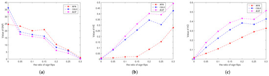
Figure 1. Average values of (a) SNR, (b) HE, and (c) HD over 50 trials vs. the noise level for all tested algorithms. We fixed $m=n=1000$ and sparsity at 10.

For the second configuration, the average values of SNR, HE, and HD over 50 trials for the signals reconstructed by all algorithms against the ratio of $m/n$ are depicted in Figure 2a, Figure 2b, and Figure 2c, respectively. We can see that Algorithm 1 performs better than the other algorithms when the ratio of $m/n$ is greater than $0.5$.

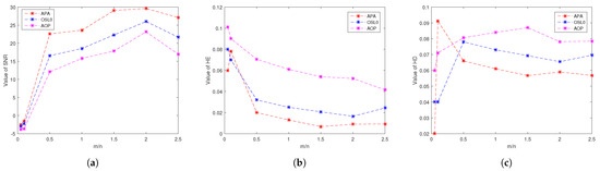
Figure 2. Average values of (a) SNR, (b) HE, and (c) HD over 50 trials vs. $m/n$ for all tested algorithms. We fix $n=1000$, the noise level at $0.05$, and sparsity at 10.

For the third configuration, the average values of SNR, HE, and HD over 50 trials for the signals reconstructed by all algorithms against the sparsity of the ideal signals are depicted in Figure 3a, Figure 3b, and Figure 3c, respectively. We can see that Algorithm 1 performs best among all the algorithms tested in our experiments.

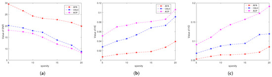
Figure 3. Average values of (a) SNR, (b) HE, and (c) HD over 50 trials vs. true sparsity s for all tested algorithms. We fix $m=n=1000$ and the noise level at $0.05$.

6. Conclusions

In this paper, we propose a robust model for the one-bit CS problem and prove that the model has a finite number of local minimizers. We propose an alternating proximal algorithm for solving the proposed model and prove the following: the sequence of the objective function decreases and converges, the set of limit points of the sequence generated from the algorithm is included in the set of critical points of the objective function, the sequence generated from the algorithm converges to a local minimizer of the objective function of the proposed model, and the sequence generated from the algorithm converges to a global minimizer of the function as long as the initial estimate is sufficiently close to any global minimizer of the function. The proposed algorithm is suitable for practical scenarios in which neither the noise level nor the sparsity of the signal are known in advance. Our algorithm possesses high time efficiency and recovery accuracy. Moreover, it performs better than other algorithms tested in our experiments when the the noise level and the sparsity of the signal is known.

References

- Boufounos, P.T.; Baraniuk, R.G. 1-bit Compressive Sensing. In Proceedings of the Conference on Information Science and Systems (CISS), Princeton, NJ, USA, 19 March 2008. [Google Scholar] [CrossRef]
- Zhou, Z.; Chen, X.; Guo, D.; Honig, M.L. Sparse channel estimation for massive MIMO with 1-bit feedback per dimension. In Proceedings of the 2017 IEEE Wireless Communications and Networking Conference (WCNC), San Francisico, CA, USA, 19–22 March 2017. [Google Scholar] [CrossRef]
- Chen, C.H.; Wu, J.Y. Amplitude-aided 1-bit compressive sensing over noisy wireless sensor networks. IEEE Wirel. Commun. Lett. 2015, 4, 473–476. [Google Scholar] [CrossRef]
- Fu, N.; Yang, L.; Zhang, J. Sub-nyquist 1-bit sampling system for sparse multiband signals. In Proceedings of the 2014 22nd European Signal Processing Conference (EUSIPCO), Lisbon, Portugal, 1–5 September 2014. [Google Scholar]
- Li, Z.; Xu, W.; Zhang, X.; Lin, J. A survey on one-bit compressed sensing: Theory and applications. Front. Comput. Sci. 2018, 12, 217–230. [Google Scholar] [CrossRef]
- Plan, Y.; Vershynin, R. One-bit compressed sensing by linear programming. Commun. Pure Appl. Math. 2013, 66, 1275–1297. [Google Scholar] [CrossRef]
- Jacques, L.; Laska, J.; Boufounos, P.T.; Baraniuk, R.G. Roubust 1-bit compressive sensing via binary stable embeddings of sparse vectors. IEEE Trans. Inf. Theory 2013, 59, 2082–2102. [Google Scholar] [CrossRef]
- Yan, M.; Yang, Y.; Osher, S. Robust 1-bit compressive sensing using adaptive outlier pursuit. IEEE Trans. Signal. Process. 2012, 60, 3868–3875. [Google Scholar] [CrossRef]
- Dai, D.Q.; Shen, L.; Xu, Y.; Zhang, N. Noisy 1-bit compressive sensing: Models and algorithms. Appl. Comput. Harmon. Anal. 2016, 40, 1–32. [Google Scholar] [CrossRef]
- Huang, J.; Jiao, Y.; Lu, X.; Zhu, L. Robust decoding from 1-bit compressive sampling with ordinary and regularized least squares. SIAM J. Sci. Comput. 2018, 40, 2062–2786. [Google Scholar] [CrossRef]
- Zhou, S.; Luo, Z.; Xiu, N.; Li, G.Y. Computing one-bit compressive sensing via double-sparsity constrained optimization. IEEE Trans. Signal. Process. 2022, 70, 1593–1608. [Google Scholar] [CrossRef]
- Rockafellar, R.T.; Wets, R. Variational Analysis, Grundlehren der Mathematischen Wissenschaften; Springer: Berlin, Germany, 1998; Volume 317. [Google Scholar]
- Mordukhovich, B. Variational Analysis and Generalized Differentiation. I. Basic Theory; Grundlehren der Mathematischen Wissenschaften; Springer: Berlin, Germany, 2006; Volume 330. [Google Scholar]
- Bauschke, H.L.; Combettes, P.L. Convex Analysis and Monotone Operator Theory in Hilbert Spaces; AMS Books in Mathematics; Springer: New York, NY, USA, 2011. [Google Scholar]
- Björck, A. Numerical Methods for Least Squares Problems; SIAM: Philadelphia, PA, USA, 1996. [Google Scholar]
- Tikhonov, A.N.; Arsenin, V.Y. Solution of Ill-Posed Problems; V. H. Winston: Washington, DC, USA, 1977. [Google Scholar]
- Daubechies, I.; Defrise, M.; Mol, C.D. An iterative thresholding algorithm for linear inverse problems with a sparsity constraint. Comm. Pure Appl. Math. 2004, 57, 1413–1457. [Google Scholar] [CrossRef]
- Figueiredo, M.A.T.; Nowak, R.D.; Wright, S.J. Gradient projection for sparse reconstruction: Application to compressed sensing and other inverse problems. IEEE J.-STSP. 2007, 1, 586–597. [Google Scholar] [CrossRef]
- Attouch, H.; Bolte, J.; Redont, P.; Soubeyran, A. Proximal alternating minimization and projection methods for nonconvex problems: An approach based on the Kurdyka-Łojasiewicz inequality. Math. Oper. Res. 2010, 35, 438–457. [Google Scholar] [CrossRef]
- Attouch, H.; Soubeyran, A. Inertia and reactivity in decision making as cognitive variational inequalities. J. Convex. Anal. 2006, 13, 207–224. [Google Scholar]
- Attouch, H.; Redont, P.; Soubeyran, A. A new class of alternating proximal minimization algorithms with costs to move. SIAM J. Optimiz. 2007, 18, 1061–1081. [Google Scholar] [CrossRef]
- Attouch, H.; Bolte, J.; Redont, P.; Soubeyran, A. Alternating proximal algorithms for weakly coupled convex minimization problems. Applications to dynamical games and PDE’s. J. Convex. Anal. 2008, 15, 485–506. [Google Scholar]
Disclaimer/Publisher’s Note: The statements, opinions and data contained in all publications are solely those of the individual author(s) and contributor(s) and not of MDPI and/or the editor(s). MDPI and/or the editor(s) disclaim responsibility for any injury to people or property resulting from any ideas, methods, instructions or products referred to in the content. |
© 2025 by the authors. Licensee MDPI, Basel, Switzerland. This article is an open access article distributed under the terms and conditions of the Creative Commons Attribution (CC BY) license (https://creativecommons.org/licenses/by/4.0/).