Article

Development of Viscosity Iterative Techniques for Split Variational-like Inequalities and Fixed Points Related to Pseudo-Contractions

1
Department of Mathematical Sciences, College of Sciences, Princess Nourah bint Abdulrahman University, Riyadh 11671, Saudi Arabia
2
Department of Mathematics, College of Science, Qassim University, Saudi Arabia
3
Department of Mathematics, Central University of Kashmir, Ganderbal 191131, Jammu and Kashmir, India
*
Authors to whom correspondence should be addressed.
Mathematics 2025, 13(17), 2896; https://doi.org/10.3390/math13172896
Submission received: 23 July 2025 / Revised: 30 August 2025 / Accepted: 4 September 2025 / Published: 8 September 2025
(This article belongs to the Special Issue Applied Functional Analysis and Applications: 2nd Edition)

Abstract

This work presents an extragradient-type iterative process combined with the viscosity method to find a common solution to a split generalized variational-like inequality, a variational inequality, and a fixed point problem associated with a family of ε -strict pseudo-contractive mappings and a nonexpansive operator in Hilbert spaces. Strong convergence of the proposed algorithm is established, with some remarks derived from the main theorem. Numerical experiments are carried out to verify the applicability of the method and provide comparative observations. The results broaden and unify a range of existing contributions in this field.

1. Introduction

Let X 1 and X 2 denote real Hilbert spaces equipped with inner product · , · and norm | · | . Let D 1 X 1 and D 2 X 2 be nonempty, closed, and convex sets. The fixed point problem (abbreviated as FPP) for a mapping T : D 1 D 1 seeks a point w D 1 satisfying T w = w . The collection of fixed points of T is represented by Fix ( T ) , that is, Fix ( T ) = { w D 1 : T w = w } .
Censor et al. [1] formulated the split feasibility problem (SFP) within the framework of finite-dimensional Hilbert spaces, motivated by applications in areas such as phase retrieval and medical imaging. The SFP is defined as follows: Find t * D 1 such that A t * D 2 , where A : X 1 X 2 is a bounded linear transformation. Since its introduction, a wide range of iterative approaches and extensions of the SFP have been actively explored in the literature; for a comprehensive discussion, refer to [2,3,4,5,6].
In this paper, we investigate the split generalized general variational-like inequality problem (abbreviated as SGGVLIP), defined as follows: find t * D 1 such that
B 1 ( w , t * ; t * ) + ψ 1 ( w , t * ) ψ 1 ( t * , t * ) 0 , w D 1 ,
and the associated point p * = A t * D 2 satisfies
B 2 ( v , p * ; p * ) + ψ 2 ( v , p * ) ψ 2 ( p * , p * ) 0 , v D 2 ,
where B j : D j × D j × D j R for j = 1 , 2 are nonlinear trifunctions, ψ j : D j × D j R for j = 1 , 2 are nonlinear bifunctions, and A : X 1 X 2 is a bounded linear operator. The set of all such solutions is denoted by Sol(SGGVLIP(1)–(2)). This formulation consists of two interconnected GGVLIPs, which are linked through the mapping p * = A t * induced by the operator A.
It is worth mentioning that the SGGVLIP framework serves as a generalization of the multiple-sets split feasibility problem and encompasses split variational inequality problems as particular instances. This formulation further extends several well-known problems, including the split zero problem, split feasibility problem, and split equilibrium problem (see, for instance, [2,4,7,8,9]).
If we set X 1 = X 2 , D 1 = D 2 , B 1 = B 2 , and ψ 1 = ψ 2 , then SGGVLIP((1)–(2)) reduces to a generalized general variational-like inequality problem (abbreviated as GGVLIP) that involves finding an element t * D 1 satisfying
B 1 ( w , t * ; t * ) + ψ 1 ( w , t * ) ψ 1 ( t * , t * ) 0 , w D 1
which is introduced by Kazmi et al. [10] and studied in [11,12].
If we set ψ 1 = 0 , then GGVLIP(3) reduces to a general variational-like inequality problem (abbreviated as GVLIP) that involves finding an element t * D 1 satisfying
B 1 ( w , t * ; t * ) 0 , w D 1 .
which was introduced by Preda et al. [13]. This formulation has notable applications in areas such as mathematical programming and equilibrium theory; see, for example, refs. [14,15,16,17,18].
Further, if we set B 1 ( w , t * ; t * ) = f t * , η ( w , t * ) , where f : D 1 X 1 and η : D 1 × D 1 X 1 and ψ 1 = 0 , then GGVLIP(3) is reduced to the variational-like inequality problem (abbreviated as VLIP) that involves finding an element t * D 1 satisfying
f t * , η ( w , t * ) 0 , w D 1 ,
which was introduced and studied by Parida et al. [19], and has applications in mathematical programming problems.
Moreover, if η ( w , t * ) = w t * for all w , t * D 1 , then the variational-like inequality problem is reduced to the classical variational inequality problem (abbreviated as VIP) that involves finding an element t * D 1 satisfying
f t * , w t * 0 , w D 1 ,
which was originally introduced by Hartman and Stampacchia [20]. The set of solutions of VIP(5) is denoted by Sol(VIP(5)).
If we set B 1 ( w , t * ; t * ) = G 1 ( t * , w ) , where G 1 : D 1 × D 1 R and ψ 1 0 , then GGVLIP(3) reduces to an equilibrium problem (abbreviated as EP) that involves finding an element t * D 1 satisfying
G 1 ( t * , w ) 0 , w D 1 ,
which was introduced by Blum and Oettli [21].
The GGVLIP is often interpreted as a trifunction equilibrium problem. As a result, the classical equilibrium problem emerges as a particular instance of this more general formulation. The equilibrium problem has gained considerable attention due to its profound influence on the development of multiple scientific and engineering disciplines. Notably, numerous classical problems have been shown to fit naturally within the equilibrium framework, offering a unified, flexible, and powerful approach for addressing challenges in nonlinear analysis, optimization, economics, finance, game theory, physics, and engineering [22,23].
Korpelevich [24] proposed the extragradient method within the setting of a Hilbert space X 1 to solve the VIP(5):
y 0 D 1 , d n = P D 1 ( y n α f y n ) , y n + 1 = P D 1 ( y n α f d n ) .
Here, α > 0 is a step-size parameter, f is assumed to be monotone and Lipschitz continuous, and P D 1 denotes the metric projection onto the convex set D 1 . Under appropriate assumptions, the generated sequence is guaranteed to converge to a solution of the VIP(5).
In 2006, Nadezkhina and Takahashi [25] proposed a modified version of the extragradient method given in (7), and they proved a weak convergence theorem to find a common element of the set of solutions to Fix ( T ) for a nonexpansive mapping and VIP(5) in the setting of Hilbert space.
Further, in 2006, Nadezhkina and Takahashi [26] introduced an alternative extragradient method that integrates the hybrid projection approach [27] with the extragradient scheme [24] and proved a strong convergence theorem to find a common element of the set of a solution to Fix ( T ) for a nonexpansive mapping and VIP(5) in the setting of Hilbert space. For further developments and extensions of this scheme, see [28].
It should be noted that, apart from the hybrid extra-gradient iterative method developed for approximating a common solution to GGVLIP(3), the VIP(5) and fixed point problem for nonlinear mappings, no strong convergence theorems for extra-gradient iterative methods have been established so far. Furthermore, the convergence analysis of such methods remains largely unexplored. Hence, the primary objective of this work is to introduce a non-hybrid extra-gradient iterative method for solving SGGVLIP((1)–(2)), VIP(5), and fixed point problems for nonlinear mappings and to establish strong convergence.
On the other hand, iterative approaches for strict pseudo-contractions are less advanced than those for nonexpansive mappings, despite the early contribution of Browder and Petryshyn in 1967 [29]. This gap may be attributed to the additional term on the right-hand side of (10), which complicates the convergence analysis of algorithms designed to find a fixed point of the strict pseudo-contraction S.
However, strict pseudo-contractions provide stronger applicability than nonexpansive mappings in solving inverse problems (see [30]). Therefore, it is interesting to develop the iterative methods for finding a common solution to SGGVLIP(1)–(2), VIP(5), and FPPs not only for nonexpansive mappings, but also for a finite family of ε -strict pseudo-contraction mappings. For further work, see, for example, [31,32] and the references therein.
Therefore, inspired by earlier works (e.g., [5,12,26,32]), in this paper, we propose an extra-gradient iterative method for approximating a common solution to SGGVLIP(1)–(2), VIP(5), and FPPs not only for nonexpansive mappings, but also for a finite family of ε -strict pseudo-contraction mappings in Hilbert spaces. Further, we prove that the sequences generated by the proposed iterative method converge strongly to the common solution to these problems. Furthermore, we derive some consequences from the main result. Finally, we discuss some numerical examples to demonstrate the applicability of the iterative algorithm. We mention the abbreviation and algebraic expression in Appendices Appendix A and Appendix B for the convenience of readers.

2. Preliminaries

In this section, we compile the key concepts and results needed for the presentation of this work. We denote strong and weak convergence by → and ⇀, respectively.
For any w 1 X 1 , a unique nearest point to w 1 in D 1 is denoted by P D 1 w 1 such that
w 1 P D 1 w 1 w 1 w 2 , w 2 D 1 .
The operator P D 1 is called the metric projection of X 1 onto D 1 . This projection is nonexpansive and satisfies
w 1 w 2 , P D 1 w 1 P D 1 w 2 P D 1 w 1 P D 1 w 2 2 , w 1 , w 2 X 1 .
Additionally, P D 1 w 1 is characterized by P D 1 w 1 D 1 and
w 1 P D 1 w 1 , w 2 P D 1 w 1 0 , w 2 D 1 .
This implies that
w 1 w 2 2 w 1 P D 1 w 1 2 + w 2 P D 1 w 1 2 , w 1 X 1 , w 2 D 1 .
In a real Hilbert space X 1 , it is known that
β w 1 + ( 1 β ) w 2 2 = β w 1 2 + ( 1 β ) w 2 2 β ( 1 β ) w 1 w 2 2 , w 1 , w 2 X 1 and β [ 0 , 1 ] ;
and
w 1 + w 2 2 w 1 2 + 2 w 2 , w 1 + w 2 , w 1 , w 2 X 1 .
A mapping S : D 1 X 1 is called an ε-strict pseudo-contraction if there exists ε [ 0 , 1 ) such that
S w 1 S w 2 2 w 1 w 2 2 + ε ( I S ) w 1 ( I S ) w 2 2 , w 1 , w 2 D 1 .
  • When ε = 0 , S becomes a nonexpansive mapping.
  • When ε = 1 , S becomes pseudo-contractive.
  • For λ ( 0 , 1 ) , if S λ I is pseudo-contractive, then S is called strongly pseudo-contractive.
Thus, the class of ε -strict pseudo-contractions lies strictly between nonexpansive and pseudo-contractive mappings. It is worth noting that the class of strongly pseudo-contractive mappings is not included within the class of ε -strict pseudo-contractions (see [29] for details).
The following properties and equivalent characterizations hold:
(i)
For all w 1 , w 2 D 1 , the condition (10) is equivalent to
S w 1 S w 2 , w 1 w 2 w 1 w 2 2 1 ε 2 ( I S ) w 1 ( I S ) w 2 2 .
(ii)
The mapping S is pseudo-contractive if and only if
S w 1 S w 2 , w 1 w 2 w 1 w 2 2 , w 1 , w 2 D 1 .
(iii)
The mapping S is strongly pseudo-contractive if and only if there exists λ ( 0 , 1 ) such that
S w 1 S w 2 , w 1 w 2 ( 1 λ ) w 1 w 2 2 , w 1 , w 2 D 1 .
Lemma 1
([33]). Let b n be a sequence of non-negative real numbers with the subsequence b n i such that b n i < b n i + 1 for all i N . Then, there exists a non-decreasing sequence { m j } N such that lim j m j = , and, for all sufficiently large j N , the following hold:
b m j b m j + 1 and b j b m j .
Moreover, m j is the largest number n in the set { 1 , 2 , 3 , , j } such that b n < b n + 1 .
Lemma 2
([31]). Assume that D is a strongly positive, self-adjoint, and bounded linear operator on a Hilbert space X 1 with a positive coefficient γ ¯ > 0 and 0 < ρ D 1 . Then, it follows that I ρ D 1 ρ γ ¯ .
Assumption 1
([10]). Let B 1 : D 1 × D 1 × D 1 R and ψ 1 : D 1 × D 1 R satisfy the following conditions:
(1)
B 1 ( w 1 , w 2 ; w 3 ) = 0 if w 1 = w 2 , w 1 , w 2 , w 3 D 1 ;
(2)
B 1 is generalized relaxed α-monotone, i.e., for any w 1 , w 2 D 1 and t ( 0 , 1 ] , we get
B 1 ( w 2 , w 1 ; w 2 ) B 1 ( w 2 , w 1 ; w 1 ) α ( w 1 , w 2 ) ,
where α : D 1 × D 1 R such that
lim t 0 α ( w 1 , t w 2 + ( 1 t ) w 1 ) t = 0 ;
(3)
B 1 ( w 2 , w 1 ; · ) is hemicontinuos, for any fixed w 1 , w 2 D 1 ;
(4)
B 1 ( · , w 1 ; w 3 ) is convex and lower semicontinuous, for any fixed w 1 , w 3 D 1 ;
(5)
B 1 ( w 1 , w 2 ; w 3 ) + B 1 ( w 2 , w 1 ; w 3 ) = 0 , for any w 1 , w 2 , w 3 D 1 ;
(6)
ψ 1 is skew-symmetric, i.e.,
ψ 1 ( w 1 , w 1 ) ψ 1 ( w 1 , w 2 ) + ψ 1 ( w 2 , w 2 ) ψ 1 ( w 2 , w 1 ) 0 , w 1 , w 2 D 1 ;
(7)
ψ 1 ( · , · ) is weakly continuous and ψ 1 ( · , w 2 ) convex for any fixed w 2 D 1 .
Now, we define ϝ r ( B 1 , ψ 1 ) : X 1 D 1 by
ϝ r ( B 1 , ψ 1 ) ( y ) = { x D 1 : B 1 ( w , x ; x ) + ψ 1 ( x , w ) ψ 1 ( w , w ) + 1 r w x , x y 0 , w D 1 } ,
where r is a positive real number.
The next lemma represents a particular instance of Lemmas 3.1–3.3, as established in [10] within the setting of a real Hilbert space.
Lemma 3
([10]). Let B 1 , ψ 1 satisfying the Assumption 1 and ϝ r ( B 1 , ψ 1 ) be defined in (11). Then, the following holds:
(i)
ϝ r ( B 1 , ψ 1 ) ( y ) is nonempty for each y X 1 ;
(ii)
ϝ r ( B 1 , ψ 1 ) is single-valued;
(iii)
ϝ r ( B 1 , ψ 1 ) is a firmly nonexpansive mapping, i.e., for all y 1 , y 2 X 1 ,
ϝ r ( B 1 , ψ 1 ) ( y 1 ) ϝ r ( B 1 , ψ 1 ) ( y 2 ) 2 ϝ r ( B 1 , ψ 1 ) ( y 1 ) ϝ r ( B 1 , ψ 1 ) ( y 2 ) , y 1 y 2 ;
(iv)
Fix ( ϝ r ( B 1 , ψ 1 ) ) = Sol(GGVLIP(1));
(v)
Sol(GGVLIP(1)) is closed and convex.
Further, suppose B 2 : D 2 × D 2 × D 2 R and ψ 2 : D 2 × D 2 × D 2 R satisfying Assumption 1. For s > 0 and y X 2 , define the mapping ϝ s ( B 2 , ψ 2 ) : X 2 D 2 as follows:
ϝ s ( B 2 , ψ 2 ) ( y ) = { x D 2 : B 2 ( w , x ; x ) + ψ 2 ( x , w ) ψ 2 ( x , x ) + 1 s w x , x y 0 , w D 2 } .
It follows that ϝ s ( B 2 , ψ 2 ) is nonempty, single-valued, firmly nonexpansive, Fix ( ϝ s ( B 2 , ψ 2 ) ) = Sol(GGVLIP(2)) and Sol(GGVLIP(2)) is closed and convex.
Lemma 4
([34]). Let S : D 1 X 1 be a ε i -strictly pseudo-contraction mapping. Then, Fix ( S ) is closed convex and it yields that P Fix ( S ) is well defined.
Lemma 5
([35]). For any x , w , y X 1 , we have
σ n x + γ n w + μ n y 2 = σ n x 2 + γ n w 2 + μ n y 2 σ n γ n x w 2 μ n γ n w y 2 σ n μ n x y 2 ,
where σ n , γ n , μ n [ 0 , 1 ] with σ n + γ n + μ n = 1 .
Lemma 6
([32]). To each i = 1 , 2 , 3 , , N , where N be an integer, consider S i : D 1 X 1 be a ε i -strictly pseudo-contraction mapping for some 0 ε i < 1 and max 1 i < N ε i < 1 with i = 1 N Fix ( S i ) . Let { φ i ( n ) } i = 1 N , for each n 0 , be a positive sequence with i = 1 N φ i ( n ) = 1 . Then, i = 1 N φ i ( n ) S i : D 1 X 1 , for each n 0 , be ε-strictly pseudo-contraction with coefficient ε = max 1 i < N ε i and Fix ( i = 1 N φ i ( n ) S i ) = i = 1 N Fix ( S i ) .
Lemma 7
([36]). Assume that { a n } is a sequence of nonnegative real numbers such that
a n + 1 ( 1 γ n ) a n + ϑ n , n 0 ,
where { γ n } is a sequence in ( 0 , 1 ) and { ϑ n } is a sequence in R such that
(i)
n = 1 γ n = ;
(ii)
lim sup n ϑ n γ n 0 or n = 1 | ϑ n | < + .
Then, lim n a n = 0 .

3. Main Outcome

Theorem 1.
Let D 1 and D 2 be nonempty closed convex subsets of Hilbert spaces X 1 and X 2 , respectively. For j = 1 , 2 , let B j : D j × D j × D j R be trifunctions, and let ψ j : D j × D j R be bifunctions satisfying Assumption 1. Let A : X 1 X 2 be a bounded linear operator. Let f : D 1 X 1  be a σ-inverse strongly monotone mapping, and let g : D 1 D 1 be a ϑ-contraction mapping. Further, let T : D 1 X 1 be a nonexpansive mapping, and for each i = 1 , 2 , 3 , , N , let S i : D 1 X 1 be an ε i -strict pseudo-contraction mapping. Let { φ i ( n ) } i = 1 N , for each n 0 , be a finite sequence of positive numbers with i = 1 N φ i ( n ) = 1 . Assume that the common solution set Γ : = i = 1 N Fix ( S i ) Fix ( T ) Sol ( SGGVLIP ( 1 ) ( 2 ) ) Sol ( VIP ( 5 ) ) . Let the sequence { y n } be generated by the following iterative process:
y 0 D 1 , u n = ϝ r n ( B 1 , ψ 1 ) y n + λ A * ϝ r n ( B 2 , ψ 2 ) I A y n , d n = P D 1 u n α n f ( u n ) , y n + 1 = η n g ( y n ) + ( 1 η n ) P D 1 σ n y n + γ n T d n + μ n i = 1 N φ i ( n ) S i y n , n 0 ,
where the control parameters satisfy the following conditions:
(i)
η n , σ n , γ n , μ n ( 0 , 1 ) and σ n + γ n + μ n = 1 ;
(ii)
lim n η n = 0 , n = 0 η n = ;
(iii)
n = 0 i = 1 N | φ i ( n ) φ i ( n 1 ) | < + ;
(iv)
0 ε i σ n c < 1 , lim n σ n = c ;
(v)
λ 0 , 1 L , where L is the spectral radius of A * A and A * is the adjoint of A;
(vi)
α n ( 0 , 2 σ ) .
Then, the sequence { y n } converges strongly to a point t * Γ , where t * = P Γ g ( t * ) .
Proof. 
We claim that { y n } is bounded. Setting s n = σ n y n + γ n T d n + μ n i = 1 N φ i ( n ) S i y n . Let t * Γ . Using the concept of non-expansive of I α n f and T, we compute
d n t * = P D 1 ( u n α n f u n ) t * ( I α n f ) u n ( I α n f ) t * u n t * ,
and thus,
T d n t * d n t * .
We calculate
u n t * 2 = ϝ r n ( B 1 , ψ 1 ) ( y n + λ A * ( ϝ r n ( B 2 , ψ 2 ) I ) A y n ) t * 2 y n + λ A * ( ϝ r n ( B 2 , ψ 2 ) I ) A y n ) t * 2 y n t * 2 + λ 2 A * ( ϝ r n ( B 2 , ψ 2 ) I ) A y n 2 + 2 λ y n t * , A * ( ϝ r n ( B 2 , ψ 2 ) I ) A y n .
Thus, we have
u n t * 2 y n t * 2 + λ 2 ( ϝ r n ( B 2 , ψ 2 ) I ) A y n , A A * ( ϝ r n ( B 2 , ψ 2 ) I ) A y n + 2 λ y n t * , A * ( ϝ r n ( B 2 , ψ 2 ) I ) A y n .
Thus,
λ 2 ( ϝ r n ( B 2 , ψ 2 ) I ) A y n , A A * ( ϝ r n ( B 2 , ψ 2 ) I ) A y n L λ 2 ( ϝ r n ( B 2 , ψ 2 ) I ) A y n , ( ϝ r n ( B 2 , ψ 2 ) I ) A y n = L λ 2 ( ϝ r n ( B 2 , ψ 2 ) I ) A y n 2 .
Assume that Π : = 2 λ y n t * , A * ( ϝ r n ( B 2 , ψ 2 ) I ) A y n ; we have
Π = 2 λ y n t * , A * ( ϝ r n ( B 2 , ψ 2 ) I ) A y n = 2 λ B ( y n t * ) , ( ϝ r n ( B 2 , ψ 2 ) I ) A y n = 2 λ B ( y n t * ) + ( ϝ r n ( B 2 , ψ 2 ) I ) A y n ( ϝ r n ( B 2 , ψ 2 ) I ) A y n , ( ϝ r n ( B 2 , ψ 2 ) I ) A y n = 2 λ { ϝ r n ( B 2 , ψ 2 ) A y n A t * , ( ϝ r n ( B 2 , ψ 2 ) I ) A y n ( ϝ r n ( B 2 , ψ 2 ) I ) A y n 2 } 2 λ 1 2 ( ϝ r n ( B 2 , ψ 2 ) I ) A y n 2 ( ϝ r n ( B 2 , ψ 2 ) I ) A y n 2 λ ( ϝ r n ( B 2 , ψ 2 ) I ) A y n 2 .
According to (17)–(19), we get
u n t * 2 y n t * 2 + λ ( L λ 1 ) ( ϝ r n ( B 2 , ψ 2 ) I ) A y n 2 .
As λ ( 0 , 1 L ) , we have
u n t * y n t * .
We compute
y n + 1 t * = η n g ( y n ) + ( 1 η n ) P D 1 s n t * η n g ( y n ) t * + ( 1 η n ) P D 1 s n t * η n g ( y n ) t * + ( 1 η n ) s n t * .
Now,
g ( y n ) t * g ( y n ) g ( t * ) + g ( t * ) t * ϑ y n t * + g ( t * ) t * .
Setting G n = i = 1 N φ i ( n ) S i and using Lemma 6, we observe that the mapping G n : D 1 X 1 is ε -strictly pseudo-contraction with ε = max 1 i < N ε i and Fix ( G n ) = i = 1 N Fix ( S i ) . Thus, according to Lemma 5, we estimate
s n t * 2 = σ n y n + γ n T d n + μ n G n y n t * 2 = σ n ( y n t * ) + γ n ( T d n t * ) + μ n ( G n y n t * ) 2 = σ n y n t * 2 + γ n T d n t * 2 + μ n G n y n t * 2 σ n γ n ( y n T d n 2 γ n μ n T d n G n y n 2 σ n μ n y n G n y n 2 σ n y n t * 2 + γ n d n t * 2 + μ n ( y n t * 2 + ε y n G n y n 2 ) σ n γ n ( y n T d n 2 γ n μ n T d n G n y n 2 σ n μ n y n G n y n 2
= ( σ n + γ n + μ n ) y n t * 2 μ n ( σ n ε ) y n G n y n 2 σ n γ n y n T d n 2 γ n μ n T d n G n y n 2 = y n t * 2 μ n ( σ n ε ) y n G n y n 2 σ n γ n y n T d n 2 γ n μ n T d n G n y n 2
that implies
s n t * y n t * .
Thus, according to (22), (23), and (26), we have
y n + 1 t * η n [ ϑ y n t * + g ( t * ) t * ] + ( 1 η n ) y n t * [ 1 η n ( 1 ϑ ) ] s n t * + η n g ( t * ) t * .
By induction, we get
y n + 1 t * max { v 0 t * , 1 1 ϑ g ( t * ) t * } , n 0 ,
which shows that { y n } is bounded, and hence, { u n } and { d n } are also bounded.
As t * Γ , therefore, we compute
y n + 1 t * 2 = η n ( g ( y n ) t * ) + ( 1 η n ) ( P D 1 s n t * ) 2 ( 1 η n ) P D 1 s n t * 2 + 2 η n ( g ( y n ) t * ) , y n + 1 t * ( 1 η n ) s n t * 2 + 2 η n g ( y n ) t * , y n + 1 t * .
Moreover, we estimate
g ( y n ) t * , y n + 1 t * = g ( y n ) t * , y n t * + g ( y n ) t * , y n + 1 y n g ( y n ) h ( t * ) y n t * + M 2 y n + 1 y n + g ( y n ) t * , y n t * ϑ y n t * 2 + M 2 y n + 1 y n + g ( y n ) t * , y n t * ,
where M = sup n g ( y n ) t * . Using (25), (28), and (29), we have
y n + 1 t * 2 ( 1 η n ( 1 2 ϑ ) ) y n t * 2 + η n M y n + 1 y n + 2 η n g ( y n ) t * , y n t * μ n ( σ n ε ) ( 1 η n ) y n G n y n 2 ( 1 η n ) σ n γ n y n T d n 2 ( 1 η n ) γ n μ n T d n G n y n 2
y n + 1 t * 2 ( 1 η n ( 1 2 ϑ ) ) y n t * 2 + η n M y n + 1 y n + 2 η n g ( y n ) t * , y n t * .
Setting q n = y n t * 2 . Consider the two cases on { q n } as follows:
Case 1. For every n m 0 where m 0 N , consider that the sequence { q n } is decreasing; therefore, it must be convergent. By applying the conditions in (30), we get
lim n y n T d n = 0 , lim n T d n G n y n = 0 and lim n y n G n y n = 0 .
Notice that { y n } is bounded; therefore, ∃ is a subsequence { v n j } of { y n } with v n j p D 1 and satisfies
lim sup n h ( t * ) t * , y n t * = lim j h ( t * ) t * , v n j t * .
Define H n = κ n v + ( 1 κ n ) G n v , v D 1 , and κ n [ ϑ , 1 ) . By applying Lemma 4, H n : D 1 X 1 is nonexpansive, and we have
y n H n y n = y n ( κ n y n + ( 1 κ n ) G n y n ) = ( κ n + ( 1 ( κ n ) y n ) ( κ n y n + ( 1 κ n ) G n y n ) = ( 1 κ n ) y n G n y n .
Thus,
lim n y n H n y n = 0 .
Applying the given conditions, we may consider that φ i ( n ) φ i as n , i . According to Lemma 6, the map G : D 1 X 1 with G v = ( i = 1 N φ i S i ) v , v D 1 is a ε -strict pseudo-contraction, and Fix ( G ) = i = 1 N Fix ( S i ) . By applying Lemma 6, given the conditions and boundedness of y n , we get
y n G y n y n G n y n + G n y n G y n y n G n y n + i = 1 N | φ i ( n ) φ i | S i y n ,
and thus,
lim n y n G y n = 0 .
As
G n y n G y n G n y n y n + y n G y n ,
which, according to (31) and (37), yields
lim n G n y n G y n = 0 .
Again, we notice that the map H = t v + ( 1 t ) G v , v D 1 and t [ ϑ , 1 ) , Fix H = Fix G . Thus, we obtain
y n H y n y n H n y n + H n y n H y n y n H n y n + κ n y n + ( 1 κ n ) H n y n t v ( 1 t ) G v y n H n y n + | κ n t | y n G y n + ( 1 κ n ) H n y n H y n .
By applying (35), (37), and (39), we have
lim n y n H y n = 0 .
As y n D 1 , therefore,
y n + 1 y n η n h y n y n + ( 1 η n ) [ σ n T d n y n + μ n y n G n y n ] .
Using the given conditions and (31), we get
lim n y n + 1 y n = 0 .
Applying (28) and (29), we estimate
y n + 1 t * 2 ( 1 η n ) s n t * 2 + 2 η n [ ϑ y n t * 2 + M 2 y n + 1 y n ] .
Using (14), (20), and (24), we compute
s n t * 2 ( 1 γ n ) y n t * 2 + γ n u n t * 2
y n t * 2 + λ ( L λ 1 ) γ n ( ϝ r n ( B 2 , ψ 2 ) I ) A y n 2
According to (43) and (45), we get
y n + 1 t * 2 ( 1 η n ) y n t * 2 + λ ( L λ 1 ) ( 1 η n ) γ n ( ϝ r n ( B 2 , ψ 2 ) I ) A y n 2 + 2 ϑ η n y n t * 2 + M η n y n + 1 y n λ ( 1 L λ ) ( 1 η n ) γ n ( ϝ r n ( B 2 , ψ 2 ) I ) A y n 2 y n t * 2 y n + 1 t * 2 + 2 ϑ η n y n t * 2 + M η n y n + 1 y n ( y n t * + y n + 1 t * ) y n y n + 1 + 2 ϑ η n y n t * 2 + M η n y n + 1 y n .
Applying the given condition and (42), we get
lim n ( ϝ r n ( B 2 , ψ 2 ) I ) A y n = 0 .
Next, we compute
u n t * 2 = ϝ r n ( B 1 , ψ 1 ) ( y n + λ A * ( ϝ r n ( B 2 , ψ 2 ) I ) A y n ) t * 2 ϝ r n ( B 1 , ψ 1 ) ( y n + λ A * ( ϝ r n ( B 2 , ψ 2 ) I ) A y n ) ϝ r n ( B 1 , ψ 1 ) t * 2 u n t * , y n + λ A * ( ϝ r n ( B 2 , ψ 2 ) I ) A y n t * = 1 2 { u n t * 2 + y n + λ A * ( ϝ r n ( B 2 , ψ 2 ) I ) A y n t * 2 ( u n t * ) [ y n + λ A * ( ϝ r n ( B 2 , ψ 2 ) I ) A y n t * ] 2 } = 1 2 { u n t * 2 + y n t * 2 u n y n λ A * ( ϝ r n ( B 2 , ψ 2 ) I ) A y n 2 } = 1 2 { u n t * 2 + y n t * 2 [ u n y n 2 + λ 2 A * ( ϝ r n ( B 2 , ψ 2 ) I ) A y n 2 2 λ u n y n , A * ( ϝ r n ( B 2 , ψ 2 ) I ) A y n ] } .
Thus,
u n t * 2 y n t * 2 u n y n 2 + 2 λ A ( z n v n ) ( ϝ r n ( B 2 , ψ 2 ) I ) A v n .
Using (44) and (49) in (43), we get
y n + 1 t * 2 ( 1 η n ) s n t * 2 + 2 η n [ ϑ y n t * 2 + M 2 y n + 1 y n ] ( 1 η n ) ( 1 γ n ) y n t * 2 + ( 1 η n ) γ n y n t * 2 γ n ( 1 η n ) u n y n 2 + 2 λ ( 1 η n ) γ n A ( z n v n ) ( ϝ r n ( B 2 , ψ 2 ) I ) A v n + 2 η n [ ϑ y n t * 2 + M 2 y n + 1 y n ] γ n ( 1 η n ) u n y n 2 y n t * 2 y n + 1 t * 2 + 2 λ ( 1 η n ) γ n A ( z n v n ) ( ϝ r n ( B 2 , ψ 2 ) I ) A v n + 2 η n [ ϑ y n t * 2 + M 2 y n + 1 y n ] ( y n t * + y n + 1 t * ) y n y n + 1 + 2 λ ( 1 η n ) γ n A ( z n v n ) ( ϝ r n ( B 2 , ψ 2 ) I ) A v n + 2 η n [ ϑ y n t * 2 + M 2 y n + 1 y n ] .
Applying given conditions (42) and (47) in (50), we get
lim n u n y n = 0 .
Further, we estimate
d n t * 2 = P D 1 ( u n α n f u n ) P D 1 ( t * α n f t * ) 2 d n t * , ( u n α n f u n ) ( t * α n f t * ) 1 2 { d n t * 2 + ( u n α n f u n ) ( t * α n f t * ) 2 ( d n u n ) + α n ( f u n f t * ) 2 } 1 2 { d n t * 2 + u n t * 2 ( d n u n ) + α n ( f u n f t * ) 2 } u n t * 2 d n u n 2 α n 2 f u n f t * 2 + 2 α n d n u n , f u n f t * u n t * 2 d n u n 2 + 2 α n d n u n f u n f t * y n t * 2 d n u n 2 + 2 α n d n u n f u n f t * .
From (24), we obtain
s n t * 2 σ n y n t * 2 + γ n d n t * 2 + μ n y n t * 2 + μ n ε y n G n y n 2 ( 1 γ n ) y n t * 2 + γ n d n t * 2 μ n ( σ n ε ) y n G n y n 2 .
From (43) and (53), we estimate
y n + 1 t * 2 ( 1 η n ) [ ( 1 γ n ) y n t * 2 + γ n d n t * 2 μ n ( σ n ε ) y n G n y n 2 ] + 2 η n [ ϑ y n t * 2 + M 2 y n + 1 y n ] ( 1 η n ) ( 1 γ n ) y n t * 2 + ( 1 η n ) γ n [ P D 1 ( u n α n f u n ) P D 1 ( t * α n f t * ) ] ( 1 η n ) μ n ( σ n ε ) y n G n y n 2 + 2 η n [ ϑ y n t * 2 + M 2 y n + 1 y n ] ( 1 η n ) ( 1 γ n ) y n t * 2 + ( 1 η n ) γ n [ u n t * 2 + α n ( α n 2 σ ) f u n f t * 2 ] ( 1 η n ) μ n ( σ n ε ) y n G n y n 2 + 2 η n [ ϑ y n t * 2 + M 2 y n + 1 y n ] ( 1 η n ) ( 1 γ n ) y n t * 2 + ( 1 η n ) γ n [ y n t * 2 + α n ( α n 2 σ ) f u n f t * 2 ] ( 1 η n ) μ n ( σ n ε ) y n G n y n 2 + 2 η n [ ϑ y n t * 2 + M 2 y n + 1 y n ] y n t * 2 + ( 1 η n ) γ n α n ( α n 2 σ ) f u n f t * 2 ( 1 η n ) μ n ( σ n ε ) y n G n y n 2 + 2 η n [ ϑ y n t * 2 + M 2 y n + 1 y n ] ;
this implies
( 1 η n ) γ n α n ( 2 σ α n ) f u n f t * 2 y n t * 2 y n + 1 t * 2 ( 1 η n ) μ n ( σ n ε ) y n G n y n 2 + 2 η n [ ϑ y n t * 2 + M 2 y n + 1 y n ] ( y n t * + y n + 1 t * ) y n y n + 1 ( 1 η n ) μ n ( σ n ε ) y n G n y n 2 + 2 η n [ ϑ y n t * 2 + M 2 y n + 1 y n ] .
By applying the given conditions, (32) and (42) in (55), we obtain
lim n f u n f t * = 0 .
Using (28), (29), (52), and (53), we compute
y n + 1 t * 2 ( 1 η n ) ( 1 γ n ) y n t * 2 + ( 1 η n ) γ n [ y n t * 2 d n u n 2 + 2 α n d n u n f u n f t * ] + ( 1 η n ) μ n ε y n G n y n 2 + 2 η n ϑ y n t * 2 + η n M y n + 1 y n + 2 η n g ( y n ) t * , y n t * ( 1 η n ) γ n d n u n 2 y n t * 2 y n + 1 t * 2 + 2 ( 1 η n ) γ n α n d n u n f u n f t * + ( 1 η n ) μ n ε y n G n y n 2 + 2 η n ϑ y n t * 2 + η n M y n + 1 y n + 2 η n g ( y n ) t * , y n t * ( y n t * + y n + 1 t * ) y n y n + 1 + 2 ( 1 η n ) γ n α n d n u n f u n f t * + ( 1 η n ) μ n ε y n G n y n 2 + 2 η n ϑ y n t * 2 + η n M y n + 1 y n + 2 η n g ( y n ) t * , y n t * .
By applying the given conditions, (31), (42) and (56), we get
lim n d n u n = 0 .
Now, we show that t * Fix ( H ) = Fix ( G ) = Fix ( G n ) = i = 1 N Fix ( S i ) . Let t * Fix ( H ) . Due to y n j t * and t * H t * , according to the Opial condition, we therefore obtain
lim inf j y n j t * < lim inf j y n j H t * lim inf j [ y n j H y n j + H y n j H t * ] lim inf j y n j t * ,
which contradicts our supposition. Hence, t * Fix ( H ) = Fix ( G ) = Fix ( G n ) = i = 1 N Fix ( S i ) . According to (31), we observe that { y n } and { d n } have the same asymptotic behaviour; therefore, ∃ is a subsequence { ϱ n j } of { d n } with ϱ n j t * . Again, from (31) and the opial condition, we see that t * Fix ( T ) . Next, we prove that t * Sol ( SGGVLIP ( 1 ) ( 2 ) ) . We set τ n : = y n + λ A * ( ( ϝ r n ( B 2 , ψ 2 ) I ) A y n . Then, u n = ϝ r n ( B 1 , ψ 1 ) τ n . For any v D 1 , we get
B 1 ( v , u n ; u n ) + ψ 1 ( v , u n ) ψ 1 ( u n , u n ) + 1 r n v u n , u n τ n 0 B 1 ( v , u n j ; u n j ) + ψ 1 ( v , u n j ) ψ 1 ( u n j , u n j ) + v u n j , u n j τ n j r n j 0
Using the concept of the generalized relaxed α -monotonicity of B 1 and (60), we get
v u n j u n j τ n j r n j 1 r n j v u n j , u n j τ n j B 1 ( v , u n j ; u n j ) ψ 1 ( v , u n j ) + ψ 1 ( u n j , u n j ) α ( u n j , v ) B 1 ( v , u n j ; v ) + ψ 1 ( u n j , u n j ) ψ 1 ( u n j , v ) .
Applying the lower semicontinuity of α in the first argument, the contiunuity of B 1 in the second argument, and the continuity of ψ 1 , we obtain
α ( t * , v ) B 1 ( v , t * ; v ) + ψ 1 ( t * , t * ) ψ 1 ( t * , v ) 0 , v D 1 .
Assume ω ς : = ( 1 ς ) t * + ς ω , ς ( 0 , 1 ] . As ω , t * D 1 , then ω ς D 1 . Therefore,
α ( t * , ω ς ) B 1 ( ω ς , t * ; ω ς ) + ψ 1 ( t * , t * ) ψ 1 ( t * , ω ς ) 0 ,
which yields that
α ( t * , ω ς ) B 1 ( ω ς , t * ; ω ς ) ψ 1 ( t * , t * ) + ψ 1 ( t * , ω ς ) ς B 1 ( ω , t * ; ω ) + ( 1 ς ) B 1 ( ω , t * ; ω ς ) ψ 1 ( t * , t * ) + ς ψ 1 ( t * , ω ) + ( 1 ς ) ψ 1 ( t * , t * ) ς [ B 1 ( ω , t * ; ω ς ) + ψ 1 ( t * , ω ) ψ 1 ( t * , t * ) ] .
As B 1 ( ω , t * ; . ) is hemicontinuous, we get
lim ς 0 { B 1 ( ω , t * ; ω ς ) + ψ 1 ( t * , ω ) ψ 1 ( t * , t * ) } lim ς 0 α ( t * , ω ς ) ς
which yields that
B 1 ( ω , t * ; t * ) + ψ 1 ( t * , ω ) ψ 1 ( t * , t * ) 0 .
Thus, t * Sol(GGVLIP(1)). Further, we prove that A t * Sol(GGVLIP(2)). As u n y n 0 , u n t * , n , and { y n } are bounded, ∃ is a subsequence { y n j } of { y n } with y n j t * and A y n j A t * because A is a bounded linear operator.
We set q n j = A y n j ϝ r n ( B 2 , ψ 2 ) A y n j . Using (47), we get lim j q n j = 0 and A y n j q n j = ϝ r n ( B 2 , ψ 2 ) A y n j . By applying Lemma 3, we get
B 2 ( A y n j q n j , v ) + ϕ 1 ( v , z n j ) ϕ 1 ( z n j , z n j ) + 1 r n j v ( A y n j q n j ) , ( A y n j q n j ) A y n j 0 , v D 1 .
By taking the limit superior in (62) to be j , using the concept of the upper semicontinuous in the first argument of B 2 , and applying the given conditions, we get
B 2 ( A t * , v ) + ϕ 1 ( v , t * ) ϕ 1 ( t * , t * ) 0 , v D 1 ,
which implies A t * Sol(GGVLIP(2)). Thus, t * Sol(SGGVLIP(1)–(2)).
Next, we show that t * Sol(VIP(5)). As lim n u n d n = 0 , ∃ { z n j } and { ϱ n j } are subsequences of { u n } and { d n } with z n j t * and ϱ n j t * .
Let
ϑ ( s ) = A ( s ) + N D 1 ( t * ) , i f t * D 1 , , i f t * D 1 ,
where N D 1 ( t * ) : = { t X 1 : t * v , t 0 , t D 1 } is the normal cone to D 1 at t * X 1 . Hence, ϑ is maximal monotone, and 0 ϑ t * t * Sol ( VIP ( 5 ) ) . Let ( t * , w ) graph ( ϑ ) . Then, w ϑ t * = A t * + N D 1 ( t * ) , and hence, w A t * N D 1 ( t * ) . Thus, t * t , w A t * 0 , t D 1 . Since d n = P D 1 ( u n α n A u n ) and t * D 1 , then
( u n α n A u n ) d n , d n t * 0 t d n , d n u n α n + A u n 0 , p D 1 .
As p t , w A p 0 , for all p D 1 and ϱ n j D 1 , the monotonicity of A, we obtain
p ϱ n j , w p ϱ n j , A t * p ϱ n j , A p p ϱ n j , ϱ n j z n j α n j + A z n j = p ϱ n j , A p A z n j + p ϱ n j , A ϱ n j A z n j p ϱ n j , ϱ n j z n j α n j p ϱ n j , A ϱ n j A z n j p ϱ n j , ϱ n j z n j α n j .
By taking j , and according to the continuity of A, we get p t * , w 0 . As ϑ is maximal monotone, t * ϑ 1 ( 0 ) , and hence, t * Sol ( VIP ( 5 ) ) . Hence, t * Γ .
As t * = P Γ h ( t * ) , according to (33), we therefore have
lim sup n h ( t * ) t * , y n t * = lim j h ( t * ) t * , v n j t * 0 .
By applying the given conditions, (30), (42), (63), and Lemma 7, we obtain q n 0 , as n . Hence, { y n } strongly converges to t * = P Γ h ( t * ) .
Case 2. Consider { q t j } to be a subsequence of { q t } with q t j < q t j + 1 , j 0 . Then, followed by Lemma 1, construct a nondecreasing sequence { m t } N with m t , as t and max { q m t , q t } q m t + 1 , t . As r t [ c , d ] ( 0 , σ 1 ) , t 0 , σ t , γ t , μ t ( 0 , 1 ) with given condition and (30), we get
lim t v m t T y m t = 0 , lim t T y m t G m t v m t = 0 and lim t v m t G m t v m t = 0 .
We apply the same steps as in case 1 to get
lim sup t h ( t * ) t * , v m t t * 0 .
As { v t } is bounded, and lim t β t = 0 , it is obtained from (32), (35), and (42)
lim t v m t + 1 v m t = 0 .
As q m t q m t + 1 , t , it is obtained from (31) that
( 1 2 ϑ ) q m t + 1 M v m t + 1 v m t + 2 h ( t * ) t * , v m t t * .
Taking t , we get q m t + 1 0 . As q m t q m t + 1 , t , then q t 0 , as t . Thus, v t 0 , as t . Hence, we have proved that the sequence { y n } strongly converges to t * = P Γ h ( t * ) .  ☐
Following this approach, we present several remarks that stem from the conclusions of Theorem 1. These remarks provide a concise overview of the theoretical results and pave the way for the broader exploration and application of the proposed iterative scheme across various mathematical and computational settings.
Remark 1.
Let T = I , I be the identity mapping, and let ε i = 0 ; that is, let S i be a finite family of nonexpansive mappings in Theorem 1. Then, Γ : = Fix ( S i ) Sol ( SGGVLIP ( 1 2 ) ) Sol ( VIP ( 5 ) ) .
Remark 2.
Let B = I , I be the identity mapping , X 1 = X 2 , D 1 = D 2 , B 1 = B 2 and ψ 1 = ψ 2 in Theorem 1. Then, Γ : = i = 1 N Fix ( S i ) Fix ( T ) Sol ( GGVLIP ( 1 ) ) Sol ( VIP ( 5 ) ) .

3.1. Numerical Example

Example 1.
Consider X 1 = X 2 = R and D 1 = D 2 = [ 0 , + ] . Define B 1 ( y 1 , w 1 ; w 1 ) = ( y 1 w 1 ) ( y 1 + 2 w 1 ) , y 1 , w 1 D 1 , B 2 ( y 2 , w 2 ; w 2 ) = ( y 2 w 2 ) ( y 2 + 2 w 2 ) , y 2 , w 2 D 2 with α ( y , w ) = ( w y ) 2 y , w D 1 , and ψ 1 ( y 1 , w 1 ) = y 1 w 1 , ψ 2 ( y 2 , w 2 ) = y 2 w 2 , y 2 , w 2 D 2 . It is obvious that B 1 , B 2 , ψ 1 and ψ 2 meet the conditions specified in Assumption 1. Additionally, assume g ( y ) = y 5 , f y = 3 y , y D 1 ; A ( y ) = y 2 , y X 1 ; T ( y ) = y 4 , y D 1 and S i ( y ) = ( 1 + i ) y , y D 1 , i = 1 , 2 , 3 . By setting r n = 2 3 , α n = { 1 5 } , λ = 1 6 , η n = { 1 10 n } , σ n = 0.7 + 0.1 n 2 , γ n = 0.2 0.2 n 2 , μ n = 0.1 + 0.1 n 2 , and ψ i = 1 3 = 1 3 , we find that the sequence generated by Algorithm 1 converges to t * = { 0 } Γ , and the algorithm simplifies to
u n = ϝ r n ( B 1 , ψ 1 ) ( y n + 1 6 A * ( ( ϝ r n ( B 2 , ψ 2 ) I ) A y n ) d n = P D 1 ( u n 1 5 f u n ) y n + 1 = η n g ( y n ) + ( 1 η n ) P D 1 [ σ n y n + γ n T d n + μ n ( φ 1 S 1 y n + φ 2 S 2 y n + φ 3 S 3 y n ) ]
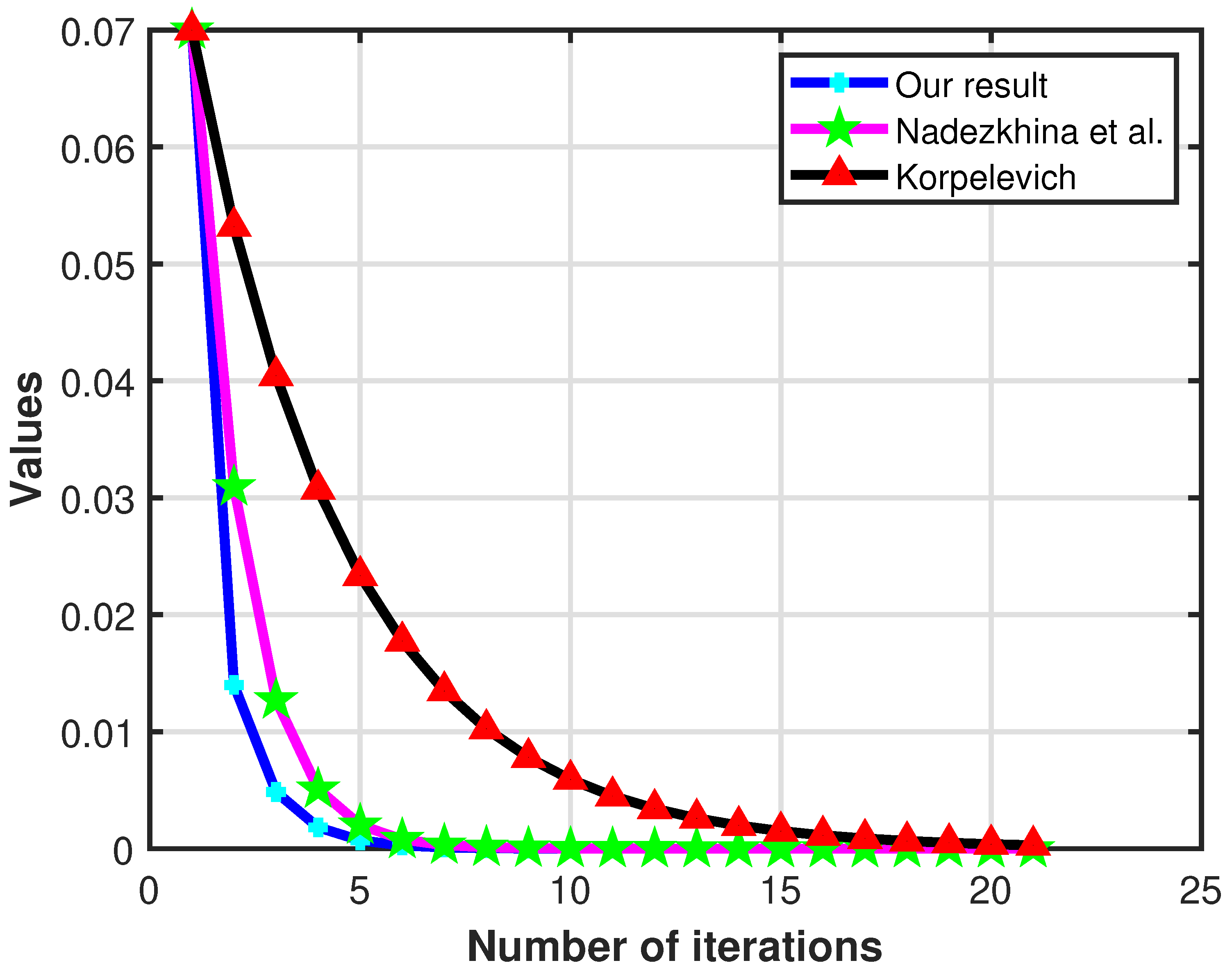
The computations and graphical analyses for the proposed algorithm were performed using MATLAB R2015(a). Figure 1 and Figure 2 depict the convergence patterns corresponding to different initial points. The stopping criterion employed is y n + 1 y n < 10 10 . Several initial values y 0 were tested, and the outcomes are summarized in Table 1 and Table 2, which also include comparisons with the results reported in [24,25]. The convergence trends are further illustrated in Figure 1 and Figure 2. From these results, it is evident that, across different initial points, the proposed algorithm generally completes computations faster (often measured in seconds) than the existing methods.
Example 2.
Consider X 1 = X 2 = C [ 0 , 1 ] as the space of all continuous real valued functions defined on [ 0 , 1 ] with the sup norm as h = max p [ 0 , 1 ] | h ( p ) | and D 1 = D 2 = { h C [ 0 , 1 ] : h ( p ) 0 , p [ 0 , 1 ] } . The metric projection of h C [ 0 , 1 ] onto D 1 is given by ( P D 1 h ) ( p ) = max { h ( p ) , 0 } , p [ 0 , 1 ] . Define B 1 ( h 1 , l 1 ; l 1 ) = ( h 1 l 1 ) ( h 1 + 2 l 1 ) , h 1 , l 1 D 1 , B 2 ( h 2 , l 2 ; l 2 ) = ( h 2 l 2 ) ( h 2 + 2 l 2 ) , h 2 , l 2 D 2 with α ( h , l ) = ( h l ) 2 h , l D 1 , and ψ 1 ( h 1 , l 1 ) = h 1 l 1 , ψ 2 ( h 2 , l 2 ) = h 2 l 2 , h 2 , l 2 D 2 . It is obvious that B 1 , B 2 , ψ 1 and ψ 2 meet the conditions specified in Assumption 1. Additionally, assume g ( h ) = h 5 , f ( h ) = 3 h , h D 1 ; A ( h ) = h 2 , h X 1 ; T ( h ) = h 4 , h D 1 and S i ( h ) = ( 1 + i ) h , h D 1 , i = 1 , 2 , 3 . By setting r n = 2 3 , α n = { 1 5 } , λ = 1 6 , η n = { 1 10 n } , σ n = 0.7 + 0.1 n 2 , γ n = 0.2 0.2 n 2 , μ n = 0.1 + 0.1 n 2 , and ψ i = 1 3 = 1 3 , we find that the sequence generated by Algorithm 1 converges to h * = { 0 } Γ .
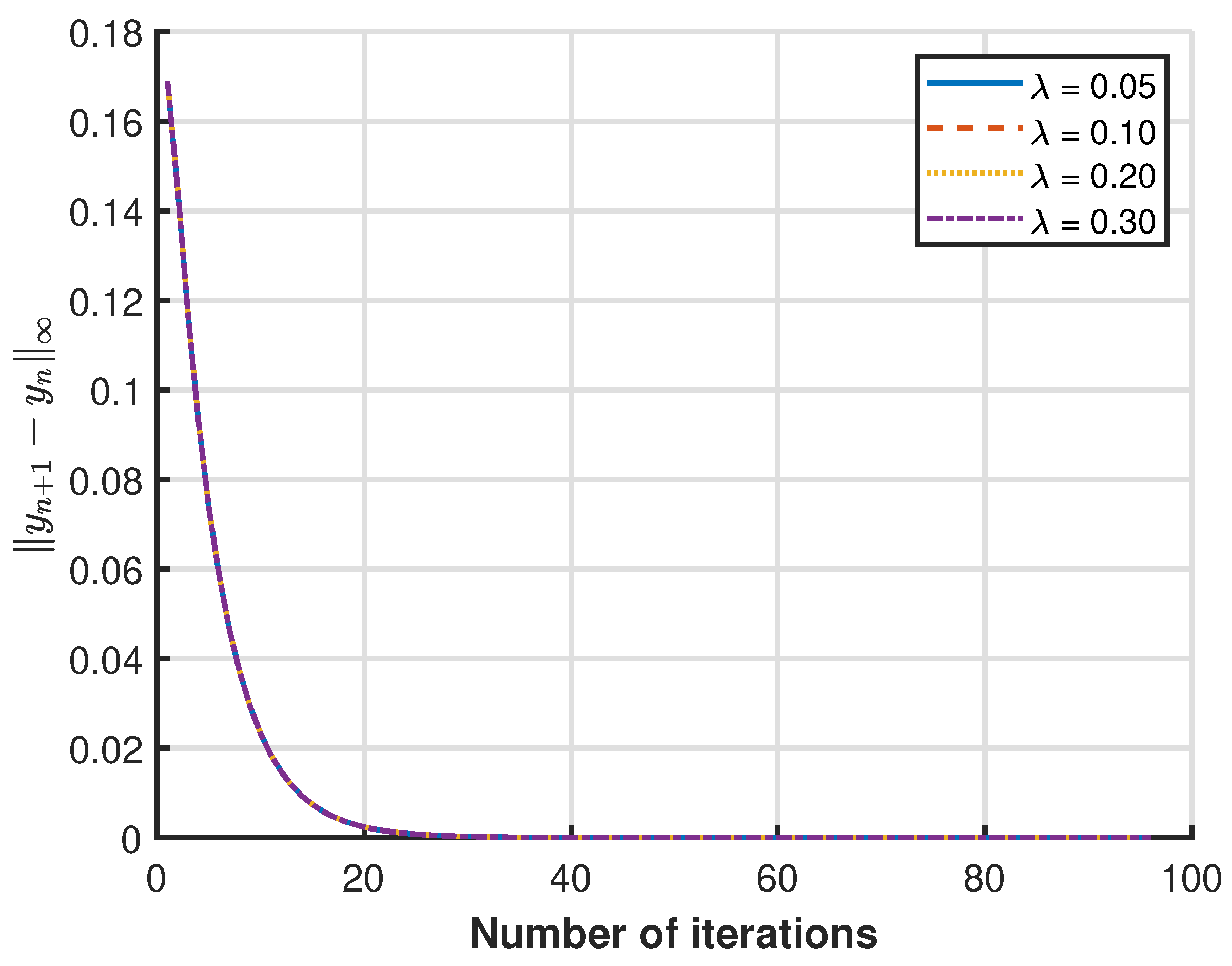
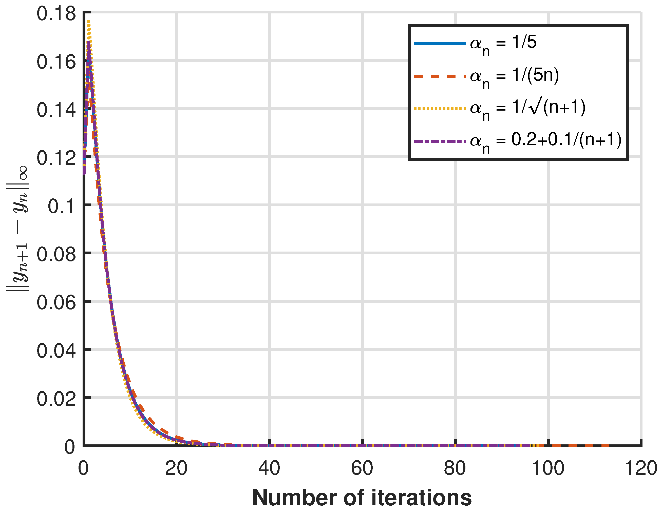
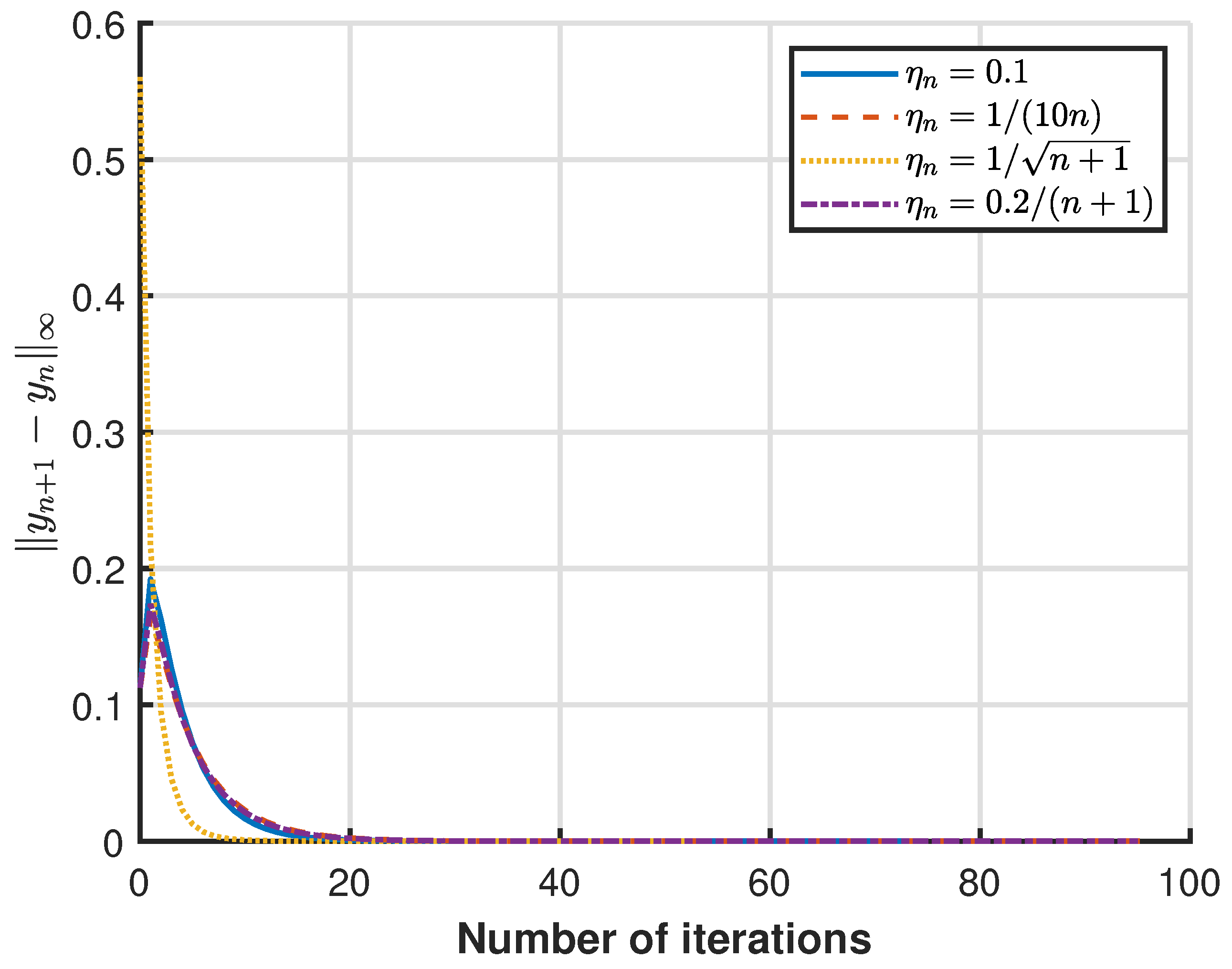
The computations and graphical visualizations for this algorithm were carried out using MATLAB R2015a on a standard HP laptop featuring an Intel Core i7 processor and 8 GB of RAM. The stopping criterion was set to y n + 1 y n < 10 10 . We analyzed the convergence for distinct initial points, and the convergence trends are illustrated in Figure 3. Further, we extended the experiment to show how convergence depends on distinct choices of control sequences: vary λ (step-size parameter); vary α n (strongly monotone scaling), and vary η n (weight between contraction mapping and other operators). We show the convergence by taking distinct values of λ , α n , and η n in Figure 4, Figure 5 and Figure 6. In the graphs, we assume y = y .

3.2. Application: Image Denoising Problem of Iteration (13)

Moreover, to evaluate the effectiveness of our approach, we applied the proposed iterative projection-based scheme to a noisy version of the test image. The original image was first corrupted with Gaussian noise, producing a degraded observation. By applying our iterative method, the noisy input was progressively refined through successive updates, resulting in a denoised image. In standard image denoising, one commonly has A = I , X 1 ( signal space ) = X 2 ( observation space ) = R m × n . Assume the trifunctions B j and bifunctions ψ j are such that their resolvent-like maps ϝ r ( B j , ψ j ) coincide with proximal maps of convex functionals F j , i.e.,
ϝ r ( B j , ψ j ) prox r F j , j = 1 , 2 ,
where
prox r F ( z ) = arg min w D F ( w ) + 1 2 r w z 2 .
Then, the iterative process (13) can be written in proximal form as
y 0 D 1 , v n = prox r n F 2 A y n , u n = prox r n F 1 y n + λ A * v n A y n , d n = P D 1 u n α n f ( u n ) , y n + 1 = η n g ( y n ) + ( 1 η n ) P D 1 σ n y n + γ n T d n + μ n i = 1 N φ i ( n ) S i y n ,
with the same control conditions (i)–(vi).
If F 2 ( z ) = 1 2 z b 2 (standard Gaussian fidelity), then
prox r F 2 ( z ) = z + r b 1 + r .
In practice, one often replaces the exact data-prox by an explicit gradient step:
prox r F 2 ( A y n ) A y n τ A y n b ,
so that with A = I , the update in (66) reduces to the familiar proximal-gradient (prox–TV) denoising iteration:
z n = y n τ ( y n b ) , u n = prox τ λ TV ( z n ) , y n + 1 = P D 1 ( u n ) .
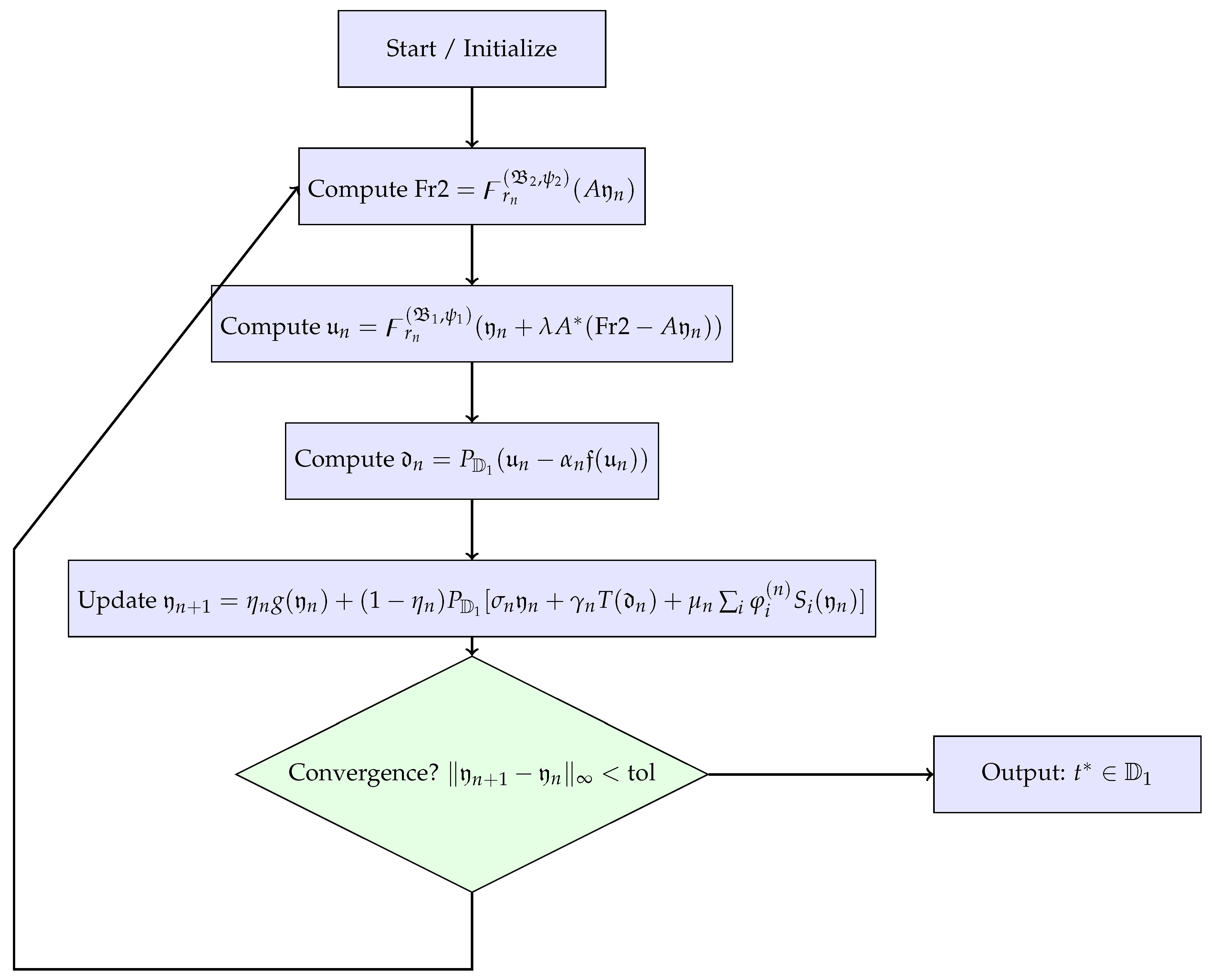
By setting the gradient step size α n 0.2 , the regularization weight (prox parameter) λ 0.1 , and the trivial convex combination weights η n 0 , σ n 0 , γ n 1 , μ n 0 , we represent the image denoising via proximal iteration in Figure 7. In Figure 7, we show that the different blurred images are degraded, along with the peak signal-to-noise ratio (PSNR); this shows the quantitatively measured image-restoring process and also the measured structural similarity index (SSIM). For the convenience of readers, we provide a flowchart of our iterative algorithm in Figure 8.

4. Conclusions

In summary, this work provides important insights into the behavior of the proposed iterative algorithm. The scheme is shown to converge strongly to a common solution for the SGGVLIPs, VIPs, and FPPs associated with a finite set of ε -strict pseudo-contractive mappings and a nonexpansive operator within a Hilbert space framework. To illustrate its practical relevance, numerical results are presented through detailed tables and graphical representations, including comparisons with existing methods and analyses of convergence trends, which collectively demonstrate the algorithm’s effectiveness and computational efficiency.
Although strong convergence is theoretically guaranteed, the algorithm’s performance can be influenced by the choice of parameters, and explicit convergence rates are not provided. Practical application may benefit from careful tuning of control sequences to enhance stability and performance. Furthermore, several avenues for future research are identified, including extending the approach to Banach spaces, establishing explicit convergence rates, and exploring inertial or stochastic modifications to broaden its applicability.

Author Contributions

G.A.: Review and Editing, Methodology; M.F.: Writing—Original Draft, Software; R.A.: Review and Editing, Conceptualization. All authors have read and agreed to the published version of the manuscript.

Funding

Princess Nourah bint Abdulrahman University Researchers Supporting Project Number (PNURSP2025R45), Princess Nourah bint Abdulrahman University, Riyadh, Saudi Arabia.

Data Availability Statement

The original contributions presented in this study are included in the article. Further inquiries can be directed to the corresponding author.

Conflicts of Interest

The authors declare that they have no competing interests.

Appendix A. Acronyms

AcronymMeaning
FPPFixed Point Problem
FPPsFixed Point Problems
VIPVariational Inequality Problem
VLIPVariational-Like Inequality Problem
GVLIPGeneral Variational-Like Inequality Problem
GGVLIPGeneralized General Variational-Like Inequality Problem
SFPSplit Feasibility Problem
GGVLIPSplit Generalized General Variational-Like Inequality Problem

Appendix B. Algebraic Details

AcronymMeaning
f : D 1 X 1 := σ -inverse strongly monotone
g : D 1 D 1 := ϑ -contraction mapping
T : D 1 X 1 := nonexpansive mapping
S i : D 1 X 1 := ε i -strict pseudo-contractions, ( i = 1 , 2 , )
A : X 1 X 2 := bounded linear operator
B j : D j × D j × D j R := be trifunctions, j = 1 , 2
ψ j : D j × D j := be bifunctions, j = 1 , 2
α n , λ , η n , σ n , γ n , μ n := are control sequences
ϝ r ( B 1 , ψ 1 ) ( y ) := { x D 1 : B 1 ( w , x ; x ) + ψ 1 ( x , w ) ψ 1 ( w , w ) + 1 r w x , x y 0 , w D 1 }
ϝ s ( B 2 , ψ 2 ) ( y ) := { x D 2 : B 2 ( w , x ; x ) + ψ 2 ( x , w ) ψ 2 ( x , x ) + 1 s w x , x y 0 , w D 2 }
s n := σ n y n + γ n T d n + μ n i = 1 N φ i ( n ) S i y n
Π := 2 λ y n t * , A * ( ϝ r n ( B 2 , ψ 2 ) I ) A y n

References

  1. Censor, Y.; Elfving, T. A multiprojection algorithms using Bragman prtojection in a product space. Numer. Algorithms 1994, 8, 221–239. [Google Scholar] [CrossRef]
  2. Censor, Y.; Bortfeld, T.; Martin, B.; Trofimov, A. A unified approach for inversion problems in intensity modulated radiation therapy. Phys. Med. Biol. 2006, 51, 2353–2365. [Google Scholar] [CrossRef]
  3. Censor, Y.; Gibali, A.; Reich, S. Algorithms for the split variational inequality problem. Numer. Algorithms 2012, 59, 301–323. [Google Scholar] [CrossRef]
  4. Combettes, P.L.; Hirstoaga, S.A. Equilibrium programming in Hilbert spaces. J. Nonlinear Convex Anal. 2005, 6, 117–136. [Google Scholar] [CrossRef]
  5. Kazmi, K.R.; Rizvi, S.H.; Farid, M. A viscosity Cesàro mean approximation method for split generalized vector equilibrium problem and fixed point problem. J. Egypt. Math. Soc. 2015, 23, 362–370. [Google Scholar] [CrossRef]
  6. Moudafi, A. Split monotone variational inclusions. J. Optim. Theory Appl. 2011, 150, 275–283. [Google Scholar] [CrossRef]
  7. Byrne, C.; Censor, Y.; Gibali, A.; Reich, S. Weak and strong convergence of algorithms for the split common null point problem. J. Nonlinear Convex Anal. 2012, 13, 759–775. [Google Scholar]
  8. Moudafi, A. The split common fixed point problem for demicontractive mappings. Inverse Probl. 2010, 26, 055007. [Google Scholar] [CrossRef]
  9. Takahashi, S.; Takahashi, W. Viscosity approximation method for equilibrium problems and fixed point problems in Hilbert space. J. Math. Anal. Appl. 2007, 331, 506–515. [Google Scholar] [CrossRef]
  10. Kazmi, K.R.; Ali, R. Hybrid projection methgod for a system of unrelated generalized mixed variational-like inequality problems. Georgian Math. J. 2019, 26, 63–78. [Google Scholar] [CrossRef]
  11. Farid, M.; Cholamjiak, W.; Ali, R.; Kazmi, K.R. A new shrinking projection algorithm for a generalized mixed variational-like inequality problem and asymptotically quasi-ϕ-nonexpansive mapping in a Banach space. RACSAM 2021, 115, 114. [Google Scholar] [CrossRef]
  12. Farid, M.; Aldosary, S.F. An Iterative approach with the inertial method for solving variational-like inequality problems with multivalued mappings in a Banach space. Symmetry 2024, 16, 139. [Google Scholar] [CrossRef]
  13. Preda, V.; Beldiman, M.; Batatoresou, A. On variational-like inequalities with generalized monotone mappings. In Generalized Convexity and Related Topics; Lecture Notes in Economics and Mathematical Systems; Springer: Berlin/Heidelberg, Germany, 2006; Volume 583, pp. 415–431. [Google Scholar] [CrossRef]
  14. Ceng, L.C.; Huan, X.Z.; Liang, Y.; Yao, J.C. On stochastic fractional differential variational inequalities general system with Lévy jumps. Commun. Nonlinear Sci. Numer. Simul. 2025, 140, 108373. [Google Scholar] [CrossRef]
  15. Ceng, L.C.; Zhu, L.J.; Yin, T.C. Modified subgradient extragradient algorithms for systems of generalized equilibria with constraints. AIMS Math. 2023, 8, 2961–2994. [Google Scholar] [CrossRef]
  16. Rehman, H.U.; Sitthithakerngkiet, K.; Seangwattana, T. Dual-Inertial Viscosity-Based Subgradient Extragradient Methods for Equilibrium Problems Over Fixed Point Sets. Math. Methods Appl. Sci. Anal. Appl. 2025, 48, 6866–6888. [Google Scholar] [CrossRef]
  17. Kankam, K.; Cholamjiak, W.; Cholamjiak, P.; Yao, J.C. Enhanced proximal gradient methods with multi inertial terms for minimization problem. J. Appl. Math. Comput. 2025. [Google Scholar] [CrossRef]
  18. Yao, J.C. The generalized quasi-variational inequality problem with applications. J. Math. Anal. 1991, 158, 139–160. [Google Scholar] [CrossRef]
  19. Parida, J.; Sahoo, M.; Kumar, A. A variational-like inequalitiy problem. Bull. Austral. Math. Soc. 1989, 39, 225–231. [Google Scholar] [CrossRef]
  20. Hartman, P.; Stampacchia, G. On some non-linear elliptic differential-functional equation. Acta Mathenatica 1966, 115, 271–310. [Google Scholar] [CrossRef]
  21. Blum, E.; Oettli, W. From optimization and variational inequalities to equilibrium problems. Math. Stud. 1994, 63, 123–145. [Google Scholar]
  22. Treanţă, S.; Pîrje, C.F.; Yao, J.C.; Upadhyay, B.B. Efficiency conditions in new interval-valued control models via modified T-objective functional approach and saddle-point criteria. Math. Model. Control 2025, 5, 180–192. [Google Scholar] [CrossRef]
  23. Wang, Y.; Li, K. Exponential synchronization of fractional order fuzzy memristor neural networks with time-varying delays and impulses. Math. Model. Control 2025, 5, 164–179. [Google Scholar] [CrossRef]
  24. Korpelevich, G.M. The extragradient method for finding saddle points and other problems. Matecon 1976, 12, 747–756. [Google Scholar] [CrossRef]
  25. Nadezhkina, N.; Takahashi, W. Strong convergence theorem by a hybrid method for nonexpansive mapping and Lipschitz continuous monotone mappings. SIAM J. Optim. 2006, 16, 1230–1241. [Google Scholar] [CrossRef]
  26. Nadezhkina, N.; Takahashi, W. Weak convergence theorem by a extragradient method for nonexpansive mappings and monotone mappings. J. Optim. Theory Appl. 2006, 128, 191–201. [Google Scholar] [CrossRef]
  27. Nakajo, K.; Takahashi, W. Strong convergence theorems for nonexpansive mappings and nonexpansive semigroups. J. Math. Anal. Appl. 2003, 279, 372–379. [Google Scholar] [CrossRef]
  28. Ceng, L.C.; Hadjisavvas, N.; Wong, N.C. Strong convergence theorem by a hybrid extragradient-like approximation method for variational inequalities and fixed point problems. J. Global Optim. 2010, 46, 635–646. [Google Scholar] [CrossRef]
  29. Browder, F.E.; Petryshyn, W.V. Construction of fixed points of nonlinear mappings in Hilbert spaces. J. Math. Anal. Appl. 1967, 20, 197–228. [Google Scholar] [CrossRef]
  30. Scherzer, O. Convergence criteria of iterative methods based on Landweber iteration for solving nonlinear problems. J. Math. Anal. Appl. 1991, 194, 911–933. [Google Scholar] [CrossRef]
  31. Marino, G.; Xu, H.K. Weak and strong convergence theorems for k-strict pseudo-contractions in Hilbert spaces. J. Math. Anal. Appl. 2007, 329, 336–349. [Google Scholar] [CrossRef]
  32. Xu, W. Iterative methods for strict pseudo-contractions in Hilbert spaces. Nonlinear Anal. 2007, 67, 2258–2271. [Google Scholar] [CrossRef]
  33. Maingé, P.E. Strong convergence of projected subgradient methods for nonsmooth and nonstrictly convex minimization. Set-Valued Anal. 2008, 16, 899–912. [Google Scholar] [CrossRef]
  34. Zhou, H.Y. Convergence theorems of fixed points for k-strict pseudo-contractions in Hilbert space. Nonlinear Anal. 2008, 69, 456–462. [Google Scholar] [CrossRef]
  35. Osilike, M.O.; Igbokewe, D.I. Weak and strong convergence theorems for fixed points of pseudo-contractions and solutions of monotone type operator equations. Comput. Math. Appl. 2000, 40, 559–567. [Google Scholar] [CrossRef]
  36. Xu, H.K. Iterative algorithms for nonlinear operators. J. Lond. Math. Soc. 2002, 66, 240–256. [Google Scholar] [CrossRef]
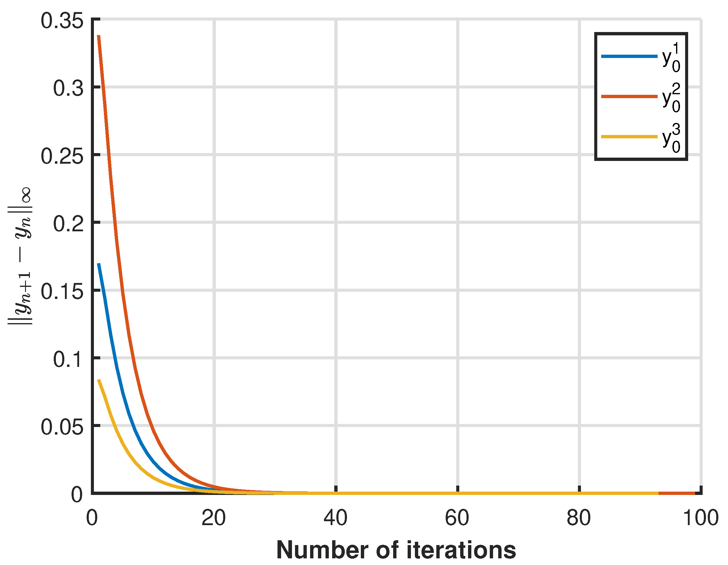
Figure 1. Graph of convergence { y n } at y 0 = 0.07 [24,25].
Mathematics 13 02896 g001
Figure 2. Graph of convergence { y n } at y 0 = 3.2 [24,25].
Mathematics 13 02896 g002
Figure 3. Graph of convergence.
Mathematics 13 02896 g003
Figure 4. Convergence for distinct values of λ .
Mathematics 13 02896 g004
Figure 5. Convergence for distinct values of { α n } .
Mathematics 13 02896 g005
Figure 6. Convergence for distinct values of { η n } .
Mathematics 13 02896 g006
Figure 7. Image denoising via proximal iteration.
Mathematics 13 02896 g007
Figure 8. Flowchart of the iterative algorithm.
Mathematics 13 02896 g008
Table 1. Comparison of our main results for initial point y 0 = 0.07 .
No. of Iter.Our ResultNadezkhina et al. [25]Korpelevich [24]
cpu Time (in s)cpu Time (in s)cpu Time (in s)
10.0140000.0309400.053200
20.0048480.0127160.040432
30.0018250.0050950.030728
40.0007070.0020150.023354
50.0002780.0007910.017749
60.0001100.0003090.013489
70.0000440.0001200.010252
80.0000180.0000470.007791
90.0000070.0000180.005921
100.0000030.0000070.004500
110.0000010.0000030.003420
120.0000000.0000010.002599
Table 2. Comparison of our main results for initial point y 0 = 3.2 .
No. of Iter.Our ResultNadezkhina et al. [25]Korpelevich [24]
cpu Time (in s)cpu Time (in s)cpu Time (in s)
10.6400001.4900002.600000
20.2216120.4972502.000000
30.0834140.1992321.400000
40.0323350.0787960.800000
50.0127120.0309200.608000
60.0050370.0120690.462080
70.0020060.0046930.351181
80.0008020.0018200.266897
90.0003210.0007040.202842
100.0001290.0002720.154160
110.0000520.0001050.117162
120.0000210.0000400.089043
130.0000080.0000160.067673
170.0000000.0000010.022577
Disclaimer/Publisher’s Note: The statements, opinions and data contained in all publications are solely those of the individual author(s) and contributor(s) and not of MDPI and/or the editor(s). MDPI and/or the editor(s) disclaim responsibility for any injury to people or property resulting from any ideas, methods, instructions or products referred to in the content.