Article

The Instability in the Dimensions of Polynomial Splines of Mixed Smoothness over T-Meshes

by
Pengxiao Wang
School of Physical and Mathematical Sciences, Nanjing Tech University, Nanjing 211816, China
Mathematics 2025, 13(17), 2886; https://doi.org/10.3390/math13172886
Submission received: 15 August 2025 / Revised: 3 September 2025 / Accepted: 3 September 2025 / Published: 6 September 2025

Abstract

Mixed-smoothness splines facilitate localized control over smoothness; however, the issue of dimensional instability in mixed-smoothness spline spaces remains unstudied in the existing literature. This paper studies such instabilities over T-meshes, where different orders of smoothness are required across interior mesh segments. Using the smoothing cofactor-conformality method, we introduce a constraint on T-meshes to derive a stable dimension formula for mixed-smoothness spline spaces. Furthermore, we show dimensional instability in cases involving T-cycles and nested T-cycles. By defining a singularity factor for each T-cycle, we demonstrate that both dimensional instabilities and structural degenerations are associated with these singularity factors. The work contributes to a deeper understanding of spline spaces defined over non-tensor-product structures.

1. Introduction

Non-Uniform Rational B-splines (NURBSs) are widely employed in computer-aided design (CAD), geometric design (CAGD), manufacturing (CAM), engineering (CAE) and approximation theory [1,2]. However, NURBSs are fundamentally based on a tensor-product structure, requiring control points to lie on a topologically rectangular grid. Local refinement inevitably results in a large number of superfluous control points, imposing significant computational burdens on NURBS models [3,4].
To overcome the limitations of NURBS, Sederberg et al. [3] introduced T-splines, a point-defined spline defined on a T-mesh. T-splines offer greater flexibility for representing free-form surfaces and can control the surface shape with fewer control points. Furthermore, a specific class of T-splines, known as analysis-suitable T-splines, has been developed. Their basis functions are linearly independent and form a partition of unity [5,6]. Scott et al. [6] also presented a greedy algorithm for implementing local refinement in analysis-suitable T-splines. In addition, Pan et al. [7,8,9] showed how to generate hierarchical T-meshes with associated locally refined B-splines, which possess the property of local linear independence, form a non-negative partition of unity, and span the resulting spaces of C s -smooth polynomial splines of degree p = 2 s + 1 . They are called RMB-splines, which are a type of locally refined spline.
There is another way to achieve local modification for tensor-product B-splines on rectangular meshes. Deng et al. first introduced the spline space over a T-mesh in [10], denoted as S ( m , n , α , β , T ) . This space comprises bi-degree ( m , n ) piecewise polynomials defined on T-mesh T with smoothness order α in the x direction and β in the y direction. Using the B-net method, Deng et al. [10] derived the dimension of S ( m , n , α , β , T ) under the constraints m 2 α + 1 and n 2 β + 1 for T-meshes without T-cycles. Huang et al. [11] obtained an equivalent dimension formula in a different form using the smoothing cofactor-conformality method [12,13]. Li et al. [14] refined the dimension formula in the same spline space by using the smoothing cofactor-conformality method under constraints involving the smoothness order, spline degree and the T-mesh structure as well. In addition, Li et al. [15] discussed the stability of the dimensions for general spline spaces, focusing their analysis on the conformality condition at a single interior vertex. Mourrain [16] introduced weighted T-meshes, over which the dimension could be computed in an explicit formula by using homological techniques. Li et al. [17] defined diagonalizable T-meshes, over which the dimensions of spline spaces are stable.
However, the study of bivariate splines on T-meshes poses an interesting challenge as the spline space dimension can depend on the geometry structure of the partition. As is known, for Morgan–Scott triangulation, the dimension of the spline space depends not only on the topological information of the partition, but also on its geometry structure [18,19,20]. Li et al. [21] and Berdinsky et al. [22] discovered the instability in the dimensions of spline spaces over certain T-meshes. In 2015, Guo et al. [23] revealed the instability of the dimension for a T-mesh with an independent simple T-cycle. Subsequently, in 2019, Li and Wang [24] demonstrated dimension instability for a T-mesh with nested T-cycles. However, the cases of instable dimensions in mixed-smoothness spline spaces over T-meshes remain unstudied.
Certain tasks require working with splines of mixed smoothness, at least locally, e.g., geometric objects containing C 0 feature lines and solutions to physical problems that show localized discontinuities. Local control over the smoothness can be very beneficial in such cases and can lead to great improvements in the quality of the output. In 2014, Mourrian [16] firstly analysed the dimension of spline spaces of different smoothness along the interior segments of a planar T-mesh by exploiting homological technique. Recently, Toshniwal and Villamizar [25] studied the stable dimensions of spline spaces of mixed smoothness along the interior edges on T-meshes via a homology-based approach. Currently, there is limited research on the dimension of mixed-smoothness spline spaces.
In this paper, we discuss the instability in the dimensions of mixed-smoothness spline spaces using the smoothing cofactor-conformality technique, which is the central novelty of this work relative to prior studies on mixed-smoothness splines. When different orders of smoothness are required across different mesh segments, we find some very interesting results. For the cases of one T-cycle and two- and three-nested T-cycles, the instability of dimension for mixed-smoothness spline spaces is associated with a geometric property depicted by a notation of a singularity factor. In addition, we give a stable dimension formula for mixed-smoothness splines over planar T-meshes via a constraint on the T-mesh using the smoothing cofactor-conformality technique.
The remainder of this paper is organized as follows. We review some definitions and notations regarding T-meshes in Section 2. In Section 3, we introduce a constraint on the T-mesh in order to obtain a stable dimension formula for mixed-smoothness spline spaces via the smoothing cofactor-conformality technique. In Section 4, we discuss the instability of the dimensions of mixed-smoothness spline spaces over certain T-meshes with a single T-cycle and two- and three-nested T-cycles respectively. Moreover, we show that dimensional instability and structural degeneration are related to a geometric property which is defined as singularity factor. Finally, conclusions are drawn in Section 5.

2. Preliminaries

In the following, we briefly review some definitions and notations of T-meshes and mixed-smoothness spline spaces over T-meshes and recall some preliminary knowledge about the smoothing cofactor method, which is a useful tool to analyse the dimensions of spline spaces. Some basic concepts in a mesh, such as segments, vertices, cells, etc., are defined as usual.

2.1. T-Meshes

A T-mesh—a generalized rectangular grid that allows T-junctions arising from T-splines—classifies its interior mesh segments (referring to maximal interior mesh segments in the following paper) into three kinds: cross-cuts (e.g., v 1 v 2 ¯ ), where both endpoints lie on mesh boundaries; rays (e.g., v 3 v 11 ¯ ) with exactly one endpoint lying on the mesh boundary; and T-segments (e.g., v 4 v 18 ¯ ) whose endpoints are both interior vertices. Correspondingly, interior vertices are also classified into three kinds: free vertices (e.g., v 21 , v 22 , v 23 ) occurring at intersections of cross-cuts or rays; mono-vertices (e.g., v 5 , v 9 , v 16 ) formed at intersections of T-segments and cross-cuts or rays; and multi-vertices (e.g., v 6 , v 15 , v 18 ) arising exclusively at intersections of T-segments. All examples are referenced from Figure 1a.
In this case, we refer to the two T-segments as T-connected; e.g, v 7 v 19 ¯ and v 14 v 16 ¯ are T-connected at vertex v 15 . A T-connected component is defined as the union of all T-connected T-segments and their vertices—for example, the union of v 4 v 18 ¯ , v 7 v 19 ¯ , v 5 v 9 ¯ , v 12 v 13 ¯ , v 14 v 16 ¯ , v 17 v 20 ¯ in Figure 1b, which is a T-connected component that must be regarded as a local structure. In particular, a free vertex (e.g., v 21 , v 22 , v 23 ) is a single T-connected component. Based on this definition, the entire T-mesh can be decomposed into multiple different T-connected components without intersections (as illustrated by the independently enclosed dotted regions in Figure 1b).

2.2. Mixed-Smoothness Spline Spaces over T-Meshes

We define the spaces of piecewise polynomial functions on a T-mesh, with bounded degrees and given smoothness. Given a T-mesh T , let F denote all the cells in T , Ω  denote the region occupied by all the cells in T and τ denote the maximal interior segments of a general planar T-mesh T .
Definition 1.
The map r : τ N is referred to as a smoothness distribution on a T-mesh T .
Using this notation, we can define the mixed-smoothness spline space S m , n r ( T ) that forms the object of our study. The goal of this paper is to analyze the dimension of the space of bi-degree splines ( m , n ) with smoothness r on a T-mesh T . From the definition of r and the following definition, it will be clear that we are interested in obtaining highly local control over the smoothness of splines in S m , n r ( T ) .
Definition 2.
Given a T-mesh T , bi-degree ( m , n ) , and smoothness distribution r , we define the mixed-smoothness spline space S m , n r ( T ) as
S m , n r ( T ) : = s ( x , y ) ϕ P m , n , ϕ F s ( x , y ) C r ( τ ) ( Ω ) s m o o t h a c r o s s τ
where P m , n is the space of all bi-degree polynomials ( m , n ) , r ( τ ) is the corresponding smoothness order for the interior segment τ, and C r ( τ ) ( Ω ) is the space consisting of all bivariate functions which are continuous on Ω with r ( τ ) continuity along corresponding interior segment τ.
Denote v i , j by each interior vertex located at ( x i , y j ) . For convenience, we will define the smoothness map r on interior segments of T as follows: for any vertical interior segment τ : x = x i (resp. horizontal interior segment τ : y = y j ), r ( τ ) = r h ( x i ) (resp. r ( τ ) = r v ( y j ) ). We will also define the horizontal and vertical smoothness at interior vertices as follows: for any v i , j , r h ( v i , j ) = r h ( x i ) and r v ( v i , j ) = r v ( y j ) .

3. A Sufficient Condition for Stable Dimension Formula for Mixed-Smoothness Spline Spaces

In this section, we will use the smoothing cofactor-conformality method to study the dimension of S m , n r ( T ) . We then derive a sufficient condition to guarantee the dimensional stability of S m , n r ( T ) when the desired order of smoothness is constrained along each interior segment. We omit the relevant proofs of the following lemmas and theorem, as their derivations are analogous to those in [14].

3.1. Two Types of Conformality Conditions Along T-Segments

Based on the smoothing cofactor-conformality method, there exists the corresponding smoothing cofactor p i ( x , y ) P m , n r v ( y j ) 1 across each horizontal grid segment and q j ( x , y ) P m r h ( x i ) 1 , n across each vertical grid segment.
As shown in Figure 2a, for each interior vertex ( x i , y j ) denoted by v i , j , the conformality condition is
( p i p i 1 ) ( y y j ) r v ( y j ) + 1 + ( q j 1 q j ) ( x x i ) r h ( x i ) + 1 = 0 .
Notice that if v i , j is a T-junction, one of the smoothing cofactors vanishes. Since ( x x i ) r h ( x i ) + 1 and ( y y j ) r v ( y j ) + 1 are prime to each other, there exist t i ( x , y ) , t i ( x , y ) P m r h ( x i ) 1 , n r v ( y j ) 1 such that
p i p i 1 = t i ( x x i ) r h ( x i ) + 1 , q j 1 q j = t j ( y y j ) r v ( y j ) + 1 .
Substituting (2) into (1), it follows that
( t i ( x , y ) + t j ( x , y ) ) ( x x i ) r h ( x i ) + 1 ( y y j ) r v ( y j ) + 1 0 .
Thus,
t i ( x , y ) t j ( x , y ) = : d i , j ( x , y ) P m r h ( x i ) 1 , n r v ( y j ) 1 ,
where d i , j ( x , y ) P m r h ( x i ) 1 , n r v ( y j ) 1 is regarded as the conformality cofactor at the interior vertex v i , j , where P m r h ( x i ) 1 , n r v ( y j ) 1 is the bi-degree polynomial space. Therefore, we find quantity relations between smoothing cofactors
p i p i 1 d i , j ( x , y ) ( x x i ) r h ( x i ) + 1 ,
and
q j q j 1 d i , j ( x , y ) ( y y j ) r v ( y j ) + 1 .
For a horizontal T-segment containing N interior vertices, the corresponding smoothing cofactors p i ( i = 1 , , N 1 ) are shown in Figure 2b. Based on the results in [14], N conformality conditions at each vertex v i , j are established:
p 1 d 1 , j ( x , y ) ( x x 1 ) r h ( x 1 ) + 1 , p 2 p 1 d 2 , j ( x , y ) ( x x 2 ) r h ( x 2 ) + 1 , p N 1 p N 2 d N 1 , j ( x , y ) ( x x N 1 ) r h ( x N 1 ) + 1 , p N 1 d N , j ( x , y ) ( x x N ) r h ( x N ) + 1 .
By summing the above equations, we derive the conformality condition along the horizontal T-segment
i = 1 N d i , j ( x , y ) ( x x i ) r h ( x i ) + 1 0 .
Similarly, the conformality condition along the vertical T-segment is
j = 1 N d i , j ( x , y ) ( y y j ) r v ( y j ) + 1 0 ,
where N denotes the number of interior vertices on the vertical T-segment.
Equations (7) and (8) are the first and second types of conformality conditions. The global conformality conditions of a T-connected component are composed of two types of conformality equation along all T-segments, and the corresponding conformality conditions of different T-connected components can be solved individually.

3.2. The Dimensions of the Two Types of Conformality Conditions

Lemma 1.
Let d i , j ( x , y ) P m r h ( x i ) 1 , n r v ( y j ) 1 . The dimension of the solution space of the linear systems
i = 1 N d i , j ( x , y ) ( x x i ) r h ( x i ) + 1 0
is d i m 1 ( N ) = ( n r v ( y j ) ) ( i = 1 N ( m r h ( x i ) ) ( m + 1 ) ) + , where x + = m a x ( x , 0 ) . The dimension of the solution space of the linear systems
j = 1 N d i , j ( x , y ) ( y y j ) r v ( y j ) + 1 0
is d i m 2 ( N ) = ( m r h ( x i ) ) ( j = 1 N ( n r v ( y j ) ) ( n + 1 ) ) + .

3.3. The Dimensions of the Spline Spaces S m , n r ( T ) on T-Mesh

Lemma 2.
Given a T-mesh T , let r be a smoothness distribution on T , C h be interior horizontal cross-cuts, C v be interior vertical cross-cuts and T k ( k = 1 , , T ) be T-connected components. Then
d i m S m , n r ( T ) = ( m + 1 ) ( n + 1 ) + τ C h ( m + 1 ) ( n r ( τ ) ) + τ C v ( n + 1 ) ( m r ( τ ) ) + k = 1 T dim T k ,
where dim T k denotes the dimension of the global conformality conditions for the k-th T-connected component.
Lemma 3.
Let T k be the k-th T-connected component, T h , k be its horizontal T-segments, T v , k be its vertical T-segments of T k and V k be all the interior vertices of T k , with each interior vertex v i , j located at ( x i , y j ) . The j-th T-segment τ j contains h j vertices including h j ( 1 ) mono-vertices and h j ( 2 ) multi-vertices except for two end vertices ( h j = h j ( 1 ) + h j ( 2 ) + 2 ). Suppose h j ( 1 ) + 1 M j if τ j is a horizontal T-segment, and h j ( 1 ) + 1 N j if τ j is a vertical T-segment; then
d i m T k = v i , j V k ( m r h ( x i ) ) ( n r v ( y j ) ) τ T h , k ( m + 1 ) ( n r ( τ ) ) τ T v , k ( m r ( τ ) ) ( n + 1 ) ,
where M j and N j are two thresholds and M j = v i , j τ j r h ( x i ) + 1 m , N j = v i , j τ j r v ( y j ) + 1 n . In particular, for a free vertex v i , j at ( x i , y j ) , d i m v i , j = ( m r h ( x i ) ) ( n r v ( y j ) ) .
Subsequently, we present the following dimension result of S m , n r ( T ) via the smoothing cofactor method.
Theorem 1.
Given a T-mesh T , let r be a smoothness distribution on T , C h be interior horizontal cross-cuts, C v be interior vertical cross-cuts, T h be horizontal T-segments, T v be vertical T-segments and V be all of the interior vertices in T , with each interior vertex v i , j located at ( x i , y j ) . The j-th T-segment τ j contains h j ( 1 ) mono-vertices except for two end vertices. Suppose h j ( 1 ) + 1 M j if τ j is a horizontal T-segment, and h j ( 1 ) + 1 N j if τ j is a vertical T-segment. Then
d i m S m , n r ( T ) = ( m + 1 ) ( n + 1 ) + v i , j V ( m r h ( x i ) ) ( n r v ( y j ) ) + ( m + 1 ) [ τ C h ( n r ( τ ) ) τ T h ( n r ( τ ) ) ] + ( n + 1 ) [ τ C v ( m r ( τ ) ) τ T v ( m r ( τ ) ) ] ,
where M j and N j are two thresholds and M j = v i , j τ j r h ( x i ) + 1 m , N j = v i , j τ j r v ( y j ) + 1 n . The summation over C h represents the sum of the "degrees of freedom" or "smoothness deficits" contributed by every interior horizontal cross-cut τ in the partition T , and the definitions of the other summation terms are analogous.

4. Dimension Instability in Mixed-Smoothness Spline Spaces over Certain T-Meshes

This section provides examples of instable dimensions in mixed-smoothness spline spaces defined over proper T-meshes. We first review results on the dimension singularity of S ( 2 , 2 , 1 , 1 , T 1 ) . Next, we discuss the instability of dimensions in spline spaces S m , n r ( T ) over certain T-meshes. We demonstrate that this instability and structural degeneration relate to a geometric property called the singularity factor.

4.1. The Dimension Singularity Condition of S ( 2 , 2 , 1 , 1 , T 1 )

Guo et al. [23] established a necessary and sufficient condition for dimension singularity in S ( 2 , 2 , 1 , 1 , T 1 ) over the T-mesh T 1 containing a T-cycle (shown in Figure 3a).
Theorem 2
([23]). The necessary and sufficient condition of singularity of d i m S ( 2 , 2 , 1 , 1 , T 1 ) is G s t = 1 , where G s t = s 5 , 1 s 5 , 4 s 2 , 1 s 2 , 4 s 2 , 6 s 2 , 3 s 5 , 6 s 5 , 3 t 5 , 1 t 5 , 4 t 2 , 1 t 2 , 4 t 2 , 6 t 2 , 3 t 5 , 6 t 5 , 3 , s i , j = x i x j , t i , j = y i y j . If G s t = 1 , the dimension of S ( 2 , 2 , 1 , 1 , T 1 ) is 30; otherwise the dimension of S ( 2 , 2 , 1 , 1 , T 1 ) is 29.
Since dimension instability depends on the value of G s t , we define this number as the singularity factor for the T-cycle. This is also a geometric condition. For the case of an N-nested T-cycle, as shown in Figure 3b, there exists a corresponding singularity factor for each simple T-cycle, denoted by a i ( i = 1 , , N ) . Li and Wang [24] proved that the dimension of S ( 2 , 2 , 1 , 1 , T N ) is unstable when N = 2 , 3 due to different values of the singularity factors a i .

4.2. The Dimension Instability of Mixed-Smoothness Spline Space over a T-Mesh Containing a T-Cycle

Example 1.
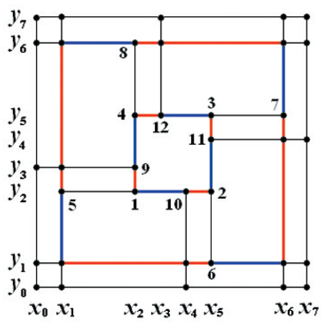
Consider the space of bi-cubic splines S 3 , 3 r ( T 1 ) over the T-mesh T 1 with smoothness distribution r shown in Figure 4a. Let x = ( x i ) i = 0 7 and y = ( y i ) y = 0 7 be two ascending sequences. The T-cycle T c 1 in T 1 consists of four T-segments: e 1 = v 5 v 2 ¯ , e 2 = v 6 v 3 ¯ , e 3 = v 7 v 4 ¯ and e 4 = v 8 v 1 ¯ . For S 3 , 3 r ( T 1 ) , the singularity factor a 1 for T c 1 is
a 1 = s 5 , 1 s 5 , 4 2 s 2 , 1 s 2 , 4 2 s 2 , 6 s 2 , 3 2 s 5 , 6 s 5 , 3 2 t 5 , 1 t 5 , 4 2 t 2 , 1 t 2 , 4 2 t 2 , 6 t 2 , 3 2 t 5 , 6 t 5 , 3 2 .
Theorem 3.
The dimension of spline space S 3 , 3 r ( T 1 ) over T-mesh T 1 shown in Figure 4a is unstable.
dim S 3 , 3 r ( T 1 ) = 44 , i f a 1 1 ( T c 1 d e g e n e r a t e s a w a y f r o m T 1 ) 45 , i f a 1 = 1 ( N o n e d e g e n e r a t i o n )
where a 1 is defined by (12). The degeneration of the T-mesh is shown in Figure 4b.
Proof. 
See Appendix A. □
Theorem 4.
The necessary and sufficient condition for the singularity of S 3 , 3 r ( T 1 ) is that the product of the ratio of the red to blue segment lengths in the outer ring and the square of the ratio of the red to blue segment lengths in the inner ring equals 1 in Figure 5.
We see that dimension instability and structural degeneration are related to the singularity factor a 1 . Numerical examples for different cases are given below.
  • Let ( x 0 , x 1 , , x 7 ) = ( 0 , 4 3 , 2 , 8 3 , 10 3 , 4 , 14 3 , 6 ) and ( y 0 ,   y 1 , , y 7 ) = ( 0 , 1 , 2 , 8 3 , 10 3 , 4 , 14 3 , 6 ) in Figure 4a. Through computation, a 1 1 ; hence, dim S 3 , 3 r ( T 1 ) = 44 and the inner T-cycle T c 1 degenerates away from T 1 .
  • Let ( x 0 , x 1 , , x 7 ) = ( 0 , 4 3 , 2 , 8 3 , 10 3 , 4 , 14 3 , 6 ) and ( y 0 ,   y 1 , , y 7 ) = ( 0 , 4 3 , 2 , 8 3 , 10 3 , 4 , 14 3 , 6 ) in Figure 4a. Through computation, a 1 = 1 ; hence, dim S 3 , 3 r ( T 1 ) = 45 and T 1 is non-degenerate.
As an extension of the structure of T 1 , we next introduce a T-mesh containing a simple T-cycle that exhibits dimension instability in the mixed-smoothness spline space.

4.3. The Dimension Instability of Mixed-Smoothness Spline Space over a T-Mesh Containing a Simple T-Cycle

Example 2.
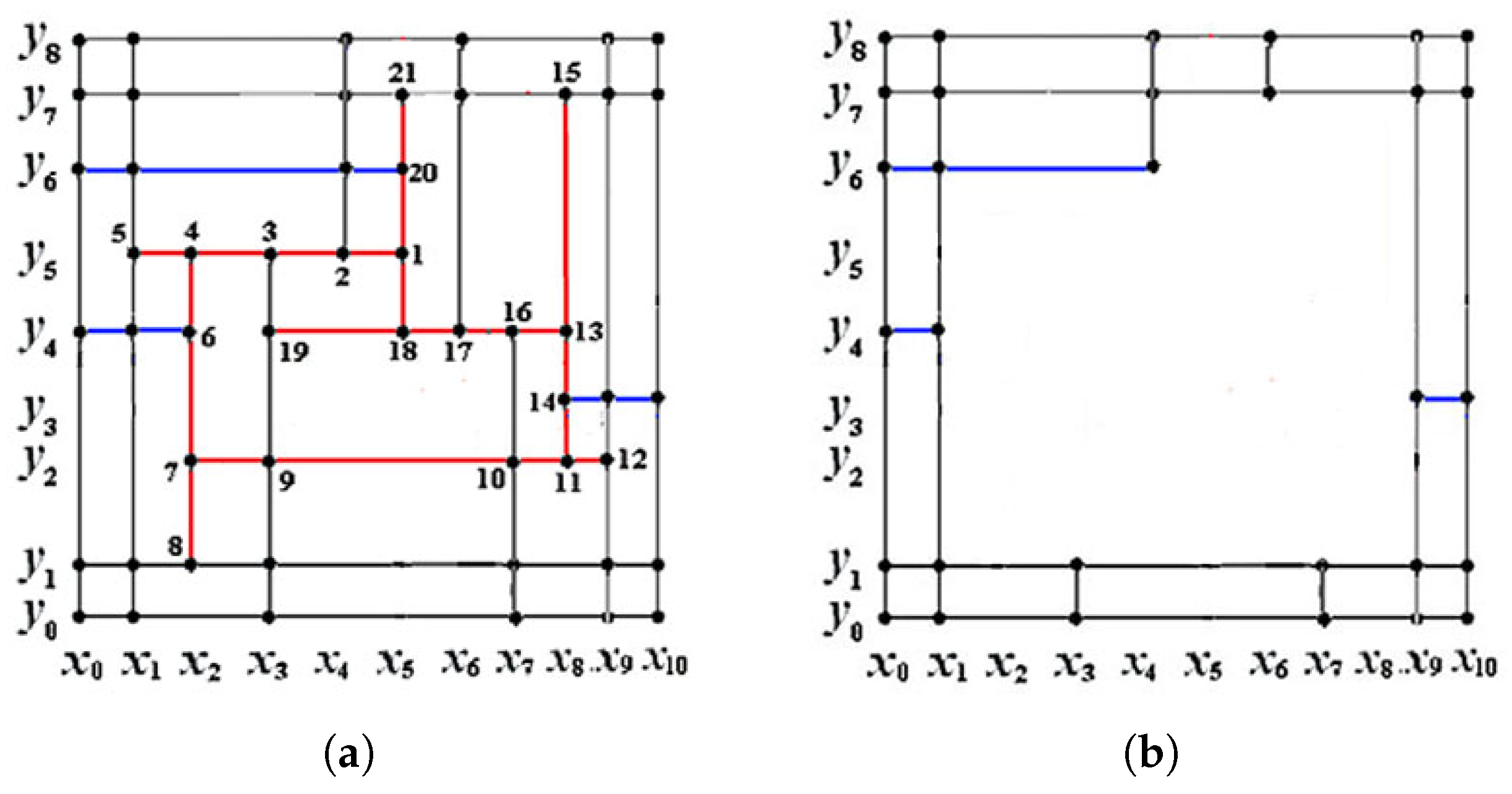
Consider the spline space S 3 , 3 r ( T ) over the T-mesh T with smoothness distribution r shown in Figure 6a. There is a simple T-cycle T s in T , which consists of six T-segments: e 1 = v 5 v 1 ¯ , e 2 = v 4 v 8 ¯ , e 3 = v 7 v 12 ¯ , e 4 = v 11 v 15 ¯ , e 5 = v 19 v 13 ¯ , e 6 = v 21 v 18 ¯ . For S 3 , 3 r ( T ) , the singularity factor a 1 for T s is
a 1 = t 4 , 6 2 t 4 , 7 t 5 , 6 2 t 5 , 7 s 7 , 8 s 6 , 8 s 3 , 8 s 5 , 7 s 5 , 6 s 3 , 5 t 2 , 3 2 t 2 , 7 t 3 , 4 2 t 4 , 7 s 2 , 9 s 2 , 7 s 2 , 3 s 7 , 8 s 3 , 8 s 8 , 9 t 4 , 5 2 t 1 , 5 t 2 , 4 2 t 1 , 2 s 4 , 5 s 3 , 5 s 1 , 5 s 2 , 4 s 2 , 3 s 1 , 2 .
Theorem 5.
The dimension of spline space S 3 , 3 r ( T ) over T-mesh T shown in Figure 6a is unstable.
dim S 3 , 3 r ( T ) = 48 , i f a 1 1 ( T s d e g e n e r a t e s a w a y f r o m T ) 49 , i f a 1 = 1 ( N o n e d e g e n e r a t i o n )
where a 1 is defined by (13). The degeneration of the T-mesh is shown in Figure 6b.
Proof. 
See Appendix B. □
We give the following numerical examples for two different cases.
  • Let ( x 0 , x 1 , , x 10 ) = ( 1 , 2 , 11 4 , 3 , 15 4 , 4 , 5 , 8 , 9 , 1367 148 , 10 ) and ( y 0 , y 1 , , y 8 ) = ( 0 , 29 38 , 1 , 2 , 8 , 17 2 , 397 50 + 21 25 , 47 5 , 10 ) in Figure 6a. Through computation, a 1 1 ; hence, dim S 3 , 3 r ( T ) = 48 and the inner T-cycle T s degenerates away from T .
  • Let ( x 0 , x 1 , , x 10 ) = ( 1 , 5 2 , 11 4 , 3 , 15 4 , 4 , 5 , 8 , 9 , 1367 148 , 10 ) and ( y 0 , y 1 , , y 8 ) = ( 0 , 29 38 , 1 , 2 , 8 , 17 2 , 397 50 + 21 25 , 47 5 , 10 ) in Figure 6a. Through computation, a 1 = 1 ; hence, dim S 3 , 3 r ( T ) = 49 and T is non-degenerate.

4.4. The Dimension Instability of Mixed-Smoothness Spline Space over a T-Mesh Containing a Two-Nested T-Cycle

Example 3.
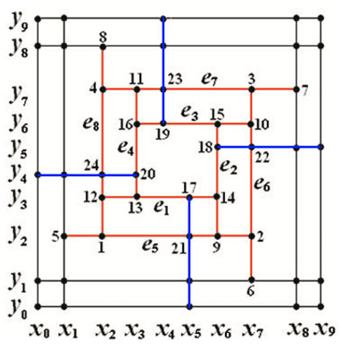
We now consider the spline space S 3 , 3 r ( T 2 ) over the T-mesh T 2 containing a two-nested T-cycle, with its smoothness distribution r as shown in Figure 7. Let x = ( x i ) i = 0 9 and y = ( y i ) y = 0 9 be two ascending sequences. There are two T-cycles, T c 1 and T c 2 , where T c 1 = { e 5 = v 5 v 2 ¯ , e 6 = v 6 v 3 ¯ , e 7 = v 7 v 4 ¯ , e 8 = v 8 v 1 ¯ } , T c 2 = { e 1 = v 12 v 14 ¯ , e 2 = v 9 v 15 ¯ , e 3 = v 10 v 16 ¯ , e 4 = v 11 v 13 ¯ } . For S 3 , 3 r ( T 2 ) , the two singularity factors a 1 and a 2 for T c 1 and T c 2 are
a 1 = s 5 , 7 2 s 1 , 7 s 2 , 5 2 s 1 , 2 t 5 , 7 2 t 1 , 7 t 2 , 5 2 t 1 , 2 s 2 , 4 2 s 2 , 8 s 4 , 7 2 s 7 , 8 t 2 , 4 2 t 2 , 8 t 4 , 7 2 t 7 , 8 ,
a 2 = s 5 , 6 2 s 2 , 6 s 3 , 5 2 s 2 , 3 t 5 , 6 2 t 2 , 6 t 3 , 5 2 t 2 , 3 s 3 , 4 2 s 3 , 7 s 4 , 6 2 s 6 , 7 t 3 , 4 2 t 3 , 7 t 4 , 6 2 t 6 , 7 .
Theorem 6.
The dimension of spline space S 3 , 3 r ( T 2 ) over T-mesh T 2 shown in Figure 7 is unstable.
d i m S 3 , 3 r ( T 2 ) = 44 , i f a 1 1 a n d a 2 1 ( B o t h T c 1 a n d T c 2 d e g e n e r a t e a w a y f r o m T 2 ) , 45 , i f a 1 = 1 a n d a 2 ( T c 2 d e g e n e r a t e s a w a y f r o m T 2 ) , 45 , i f a 1 1 a n d a 2 = 1 ( N o n e d e g e n e r a t i o n ) .
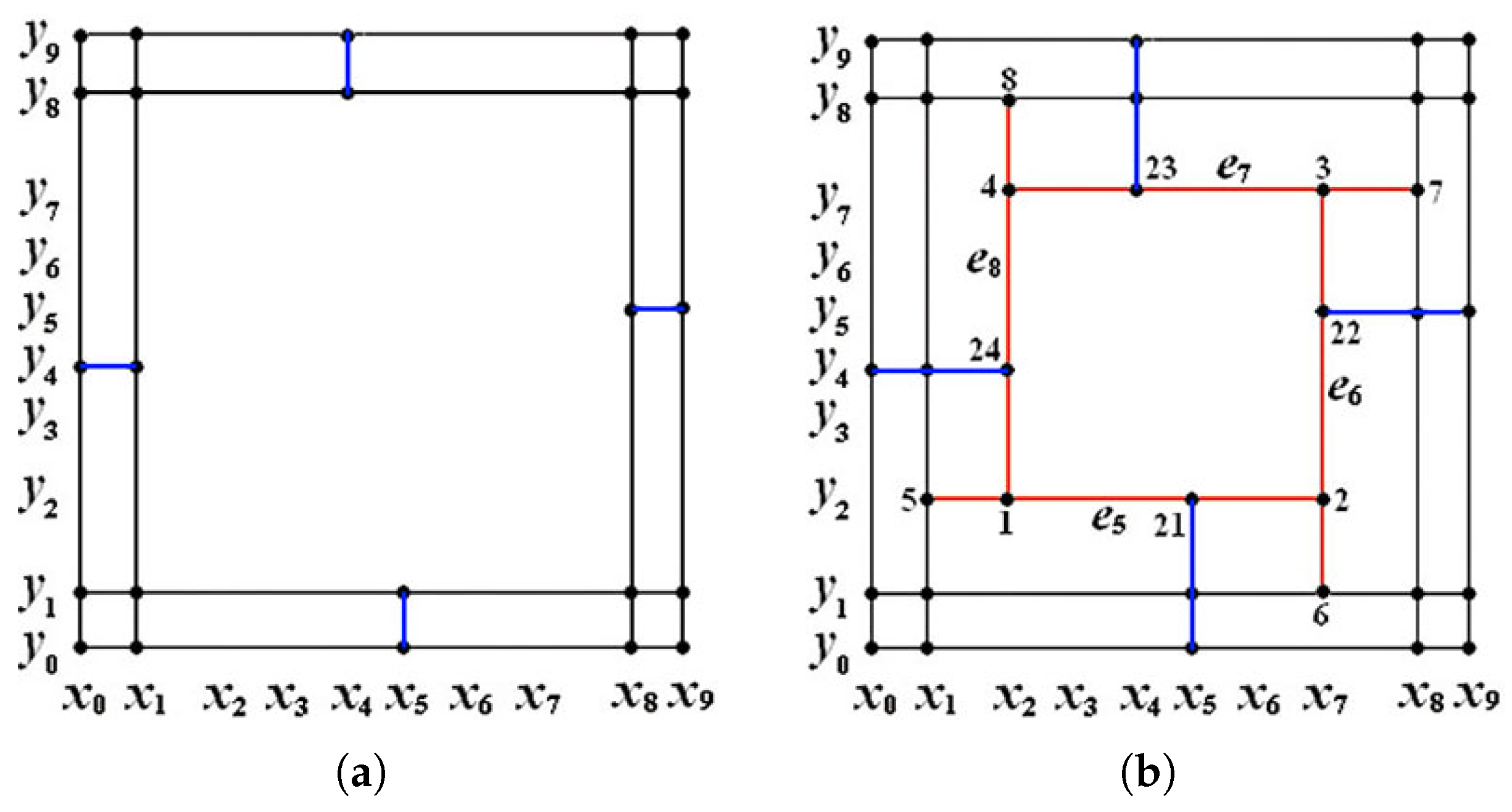
where a 1 and a 2 are defined by (14) and (15). The T-mesh’s degeneration for two different cases is shown in Figure 8.
Proof. 
See Appendix C. □
We see that dimension instability and structural degeneration relate to the singularity factor value of each T-cycle. We provide four numerical examples for different cases.
  • Let ( x 0 , x 1 , , x 9 ) = ( 2 , 1 , 4 3 , 2 , 8 3 , 10 3 , 11 3 , 14 3 , 22 3 , 8 ) and ( y 0 ,   y 1 , , y 9 ) = ( 2 , 4 3 , 4 3 , 2 , 8 3 , 10 3 , 4 , 14 3 , 22 3 , 8 ) in Figure 7. Through computation, a 1 1 and a 2 1 ; hence, dim S 3 , 3 r ( T 2 ) = 44 and two T-cycles degenerate away from T 2 .
  • Let ( x 0 , x 1 , , x 9 ) = ( 2 , 4 3 , 4 3 , 2 , 8 3 , 10 3 , 11 3 , 14 3 , 22 3 , 8 ) and ( y 0 ,   y 1 , , y 9 ) = ( 2 , 4 3 , 4 3 , 2 , 8 3 , 10 3 , 4 , 14 3 , 22 3 , 8 ) in Figure 7. Through computation, a 1 = 1 and a 2 1 ; hence, dim S 3 , 3 r ( T 2 ) = 45 and the inner T-cycle T c 2 degenerates away from T 2 .
  • Let ( x 0 , x 1 , , x 9 ) = ( 2 , 4 3 , 4 3 , 2 , 8 3 , 10 3 , 4 , 14 3 , 22 3 , 8 ) and ( y 0 ,   y 1 , , y 9 ) = ( 2 , 4 3 , 4 3 , 2 , 8 3 , 10 3 , 4 , 14 3 , 22 3 , 8 ) in Figure 7. Through computation, a 1 = 1 and a 2 = 1 ; hence, dim S 3 , 3 r ( T 2 ) = 45 and the inner T-cycle T c 2 degenerates away from T 2 .
  • Let ( x 0 , x 1 , , x 9 ) = ( 2 , 5 3 , 4 3 , 2 , 8 3 , 10 3 , 4 , 14 3 , 22 3 , 8 ) and ( y 0 ,   y 1 , , y 9 ) = ( 2 , 4 3 , 4 3 , 2 , 8 3 , 10 3 , 4 , 14 3 , 22 3 , 8 ) in Figure 7. Through computation, a 1 1 and a 2 = 1 ; hence, dim S 3 , 3 r ( T 2 ) = 45 and T 2 is non-degenerate.

4.5. The Dimension Instability of Mixed-Smoothness Spline Spaces over a T-Mesh Containing a Three-Nested T-Cycle

Example 4.
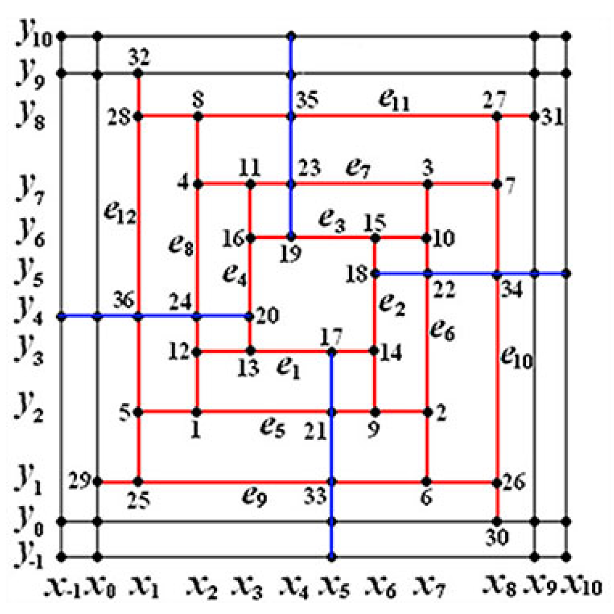
Figure 9 shows a T-mesh containing a three-nested T-cycle T 3 , formed by adding a new T-cycle outside the previously mentioned two-nested T-cycle in T 2 . We rename the three T-cycles as follows:
T c 1 = { e 9 = v 29 v 26 ¯ , e 10 = v 30 v 27 ¯ , e 11 = v 31 v 28 ¯ , e 12 = v 32 v 25 ¯ } ,
T c 2 = { e 5 = v 5 v 2 ¯ , e 6 = v 6 v 3 ¯ , e 7 = v 7 v 4 ¯ , e 8 = v 8 v 1 ¯ } ,
T c 3 = { e 1 = v 12 v 14 ¯ , e 2 = v 9 v 15 ¯ , e 3 = v 10 v 16 ¯ , e 4 = v 11 v 13 ¯ } .
For the spline space of S 3 , 3 r ( T 3 ) , the three singularity factors a 1 , a 2 and a 3 for T c 1 , T c 2 and T c 3 are
a 1 = s 5 , 8 2 s 0 , 8 s 1 , 5 2 s 0 , 1 t 5 , 8 2 t 0 , 8 t 1 , 5 2 t 0 , 1 s 1 , 4 2 s 1 , 9 s 4 , 8 2 s 8 , 9 t 1 , 4 2 t 1 , 9 t 4 , 8 2 t 8 , 9 ,
a 2 = s 5 , 7 2 s 1 , 7 s 2 , 5 2 s 1 , 2 t 5 , 7 2 t 1 , 7 t 2 , 5 2 t 1 , 2 s 2 , 4 2 s 2 , 8 s 4 , 7 2 s 7 , 8 t 2 , 4 2 t 2 , 8 t 4 , 7 2 t 7 , 8 ,
a 3 = s 5 , 6 2 s 2 , 6 s 3 , 5 2 s 2 , 3 t 5 , 6 2 t 2 , 6 t 3 , 5 2 t 2 , 3 s 3 , 4 2 s 3 , 7 s 4 , 6 2 s 6 , 7 t 3 , 4 2 t 3 , 7 t 4 , 6 2 t 6 , 7 .
Conjecture 1.
The dimension of spline space S 3 , 3 r ( T 3 ) over the T-mesh T 3 shown in Figure 9 is unstable.
S 3 , 3 r ( T 3 ) = 44 , i f a 1 1 , a 2 1 a n d a 3 1 ( A l l T c 1 , T c 2 a n d T c 3 d e g e n e r a t e a w a y f r o m T 3 ) , 45 , i f a 1 = 1 , a 2 a n d a 3 ( B o t h T c 2 a n d T c 3 d e g e n e r a t e a w a y f r o m T 3 ) , 45 , i f a 1 1 , a 2 = 1 a n d a 3 ( T c 3 d e g e n e r a t e s a w a y f r o m T 3 ) , 45 , i f a 1 1 , a 2 1 a n d a 3 = 1 ( N o n e d e g e n e r a t i o n ) .
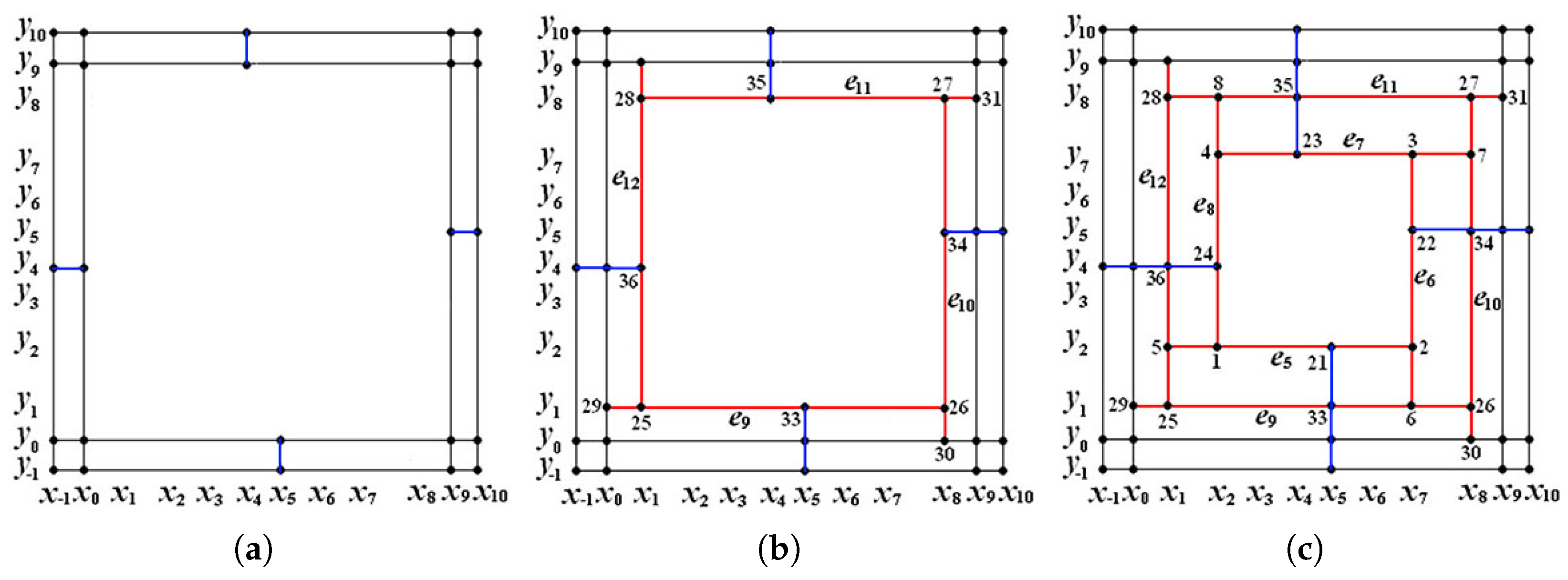
where a 1 , a 2 and a 3 are defined by (16), (17) and (18). The T-mesh’s degeneration in three different cases is shown in Figure 10.
Analysis. See Appendix D.
We provide numerical examples for various degeneration cases of the T-mesh containing a three-nested T-cycle, as detailed below.
  • Let ( x 1 , x 0 , , x 10 ) = ( 30 , 76 3 , 4 3 , 4 3 , 2 , 8 3 , 3 , 4 , 14 3 , 22 3 , 94 3 , 35 ) and ( y 1 ,   y 0 , , y 10 ) = ( 30 , 76 3 , 4 3 , 4 3 , 2 , 8 3 , 10 3 , 4 , 14 3 , 22 3 , 94 3 , 35 ) in Figure 9. Through computation, a 1 1 , a 2 1 and a 3 1 , b 1 = 0.6227 ; hence, dim S 3 , 3 r ( T 3 ) = 44 and three T-cycles degenerate away from T 3 .
  • Let ( x 1 , x 0 , , x 10 ) = ( 30 , 76 3 , 4 3 , 4 3 , 2 , 8 3 , 10 3 , 4 , 5 , 22 3 , 94 3 , 35 ) and ( y 1 ,   y 0 , , y 10 ) = ( 30 , 76 3 , 4 3 , 4 3 , 2 , 8 3 , 10 3 , 4 , 14 3 , 22 3 , 94 3 , 35 ) in Figure 9. Through computation, a 1 = 1 , a 2 1 and a 3 1 , b 1 = 0.6343 ; hence, dim S 3 , 3 r ( T 3 ) = 45 , both T c 2 and T c 3 degenerate away from T 3 .
  • Let ( x 1 , x 0 , , x 10 ) = ( 30 , 76 3 , 4 3 , 4 3 , 2 , 8 3 , 10 3 , 11 3 , 14 3 , 22 3 , 94 3 , 35 ) and ( y 1 ,   y 0 , , y 10 ) = ( 30 , 76 3 , 4 3 , 4 3 , 2 , 8 3 , 10 3 , 4 , 14 3 , 22 3 , 94 3 , 35 ) in Figure 9. Through computation, a 1 = 1 , a 2 = 1 and a 3 1 , b 1 = 0.4082 ; hence, dim S 3 , 3 r ( T 3 ) = 45 , both T c 2 and T c 3 degenerate away from T 3 .
  • Let ( x 1 , x 0 , , x 10 ) = ( 30 , 76 3 , 4 3 , 4 3 , 2 , 8 3 , 10 3 , 4 , 14 3 , 22 3 , 94 3 , 35 ) and ( y 1 ,   y 0 , , y 10 ) = ( 30 , 76 3 , 4 3 , 4 3 , 2 , 8 3 , 10 3 , 4 , 14 3 , 22 3 , 94 3 , 35 ) in Figure 9. Through computation, a 1 = 1 , a 2 = 1 and a 3 = 1 , b 1 = 0.4082 ; hence, dim S 3 , 3 r ( T 3 ) = 45 , both T c 2 and T c 3 degenerate away from T 3 .
  • Let ( x 1 , x 0 , , x 10 ) = ( 5 , 4 , 1 , 4 , 5 , 7 , 11 , 13 , 14 , 16 , 28 , 30 ) and ( y 1 ,   y 0 , , y 10 ) = ( 5 , 4 , 1 , 4 , 5 , 7 , 11 , 13 , 14 , 16 , 28 , 30 ) in Figure 9. Through computation, a 1 = 1 , a 2 1 and a 3 = 1 , b 1 = 1.3777 ; hence, dim S 3 , 3 r ( T 3 ) = 45 , both T c 2 and T c 3 degenerate away from T 3 .
  • Let ( x 1 , x 0 , , x 10 ) = ( 4 , 3 , 4 3 , 4 3 , 7 3 , 8 3 , 10 3 , 4 , 14 3 , 22 3 , 94 3 , 35 ) and ( y 1 ,   y 0 , , y 10 ) = ( 30 , 76 3 , 4 3 , 4 3 , 2 , 8 3 , 10 3 , 4 , 14 3 , 22 3 , 94 3 , 35 ) in Figure 9. Through computation, a 1 1 , a 2 = 1 and a 3 1 , b 1 = 1.7699 ; hence, dim S 3 , 3 r ( T 3 ) = 45 , T c 3 degenerates away from T 3 .
  • Let ( x 1 , x 0 , , x 10 ) = ( 3 , 2 , 4 3 , 4 3 , 2 , 8 3 , 10 3 , 4 , 14 3 , 22 3 , 94 3 , 35 ) and ( y 1 ,   y 0 , , y 10 ) = ( 30 , 76 3 , 4 3 , 4 3 , 2 , 8 3 , 10 3 , 4 , 14 3 , 22 3 , 94 3 , 35 ) in Figure 9. Through computation, a 1 1 , a 2 = 1 and a 3 = 1 , b 1 = 3.9650 ; hence, dim S 3 , 3 r ( T 3 ) = 45 , T c 3 degenerates away from T 3 .
  • Let ( x 1 , x 0 , , x 10 ) = ( 30 , 76 3 , 0 , 4 3 , 2 , 8 3 , 10 3 , 4 , 14 3 , 22 3 , 94 3 , 35 ) and ( y 1 ,   y 0 , , y 10 ) = ( 30 , 76 3 , 4 3 , 4 3 , 2 , 8 3 , 10 3 , 4 , 14 3 , 22 3 , 94 3 , 35 ) in Figure 9. Through computation, a 1 1 , a 2 1 and a 3 = 1 , b 1 = 0.8464 ; hence, dim S 3 , 3 r ( T 3 ) = 45 , T 3 is non-degenerate.

5. Conclusions

In this paper, we analyse the dimensions of the spline space S m , n r ( T ) that are piecewise bi-degree polynomials ( m , n ) with smoothness r across interior segments of a general planar T-mesh T , where r denotes a smoothness distribution on T . We establish a sufficient condition to guarantee the dimensional stability of S m , n r ( T ) . Furthermore, we study dimension instability in spline spaces with mixed smoothness over specific T-meshes, including T-cycle, simple T-cycle, and two- and three-nested T-cycles. The results show that dimension instability and structural degeneration relate to a geometric property defined by a singularity factor. In the future, we will discuss dimension instability and structural degeneration for more spline spaces.

Funding

This work was supported by the Natural Science Foundation of the Higher Education Institutions of Jiangsu Province (No. 21KJB110016) and the Philosophy and Social Science Foundation of the Higher Education Institutions of Jiangsu Province (No. 2022SJYB0217).

Data Availability Statement

No new data were created or analysed in this study. Data sharing is not applicable to this article.

Conflicts of Interest

The author declares no conflicts of interest.

Appendix A

Proof of Theorem 3.
Using the smoothing cofactor-conformality method, the conformality conditions of smoothing cofactors on each T-segment can be transformed into two types of conformality conditions. Let d i ( i = 1 , , 8 ) be the conformality cofactor at the interior vertex v i ( i = 1 , , 8 ) and d i , 1 + d i , 2 x ( i = 10 , 12 ) , d i , 1 + d i , 2 y ( i = 9 , 11 ) be the conformality cofactor at the interior vertex v i ( i = 9 , , 12 ) in Figure 4a of the main text. For T c 1 , every T-segment satisfies a conformality condition:
d 5 ( x x 1 ) 3 + d 1 ( x x 2 ) 3 + ( d 10 , 1 + d 10 , 2 x ) ( x x 4 ) 2 + d 2 ( x x 5 ) 3 0 ,
d 6 ( y y 1 ) 3 + d 2 ( y y 2 ) 3 + ( d 11 , 1 + d 11 , 2 y ) ( y y 4 ) 2 + d 3 ( y y 5 ) 3 0 ,
d 7 ( x x 6 ) 3 + d 3 ( x x 5 ) 3 + ( d 12 , 1 + d 12 , 2 x ) ( x x 3 ) 2 + d 4 ( x x 2 ) 3 0 ,
d 8 ( y y 6 ) 3 + d 4 ( y y 5 ) 3 + ( d 9 , 1 + d 9 , 2 y ) ( y y 3 ) 2 + d 1 ( y y 2 ) 3 0 .
Each conformality condition equates to a linear system. For instance, (A1) yields A d = 0 , where
A = 1 1 1 1 0 3 x 1 3 x 2 3 x 5 2 x 4 1 3 x 1 2 3 x 2 2 3 x 5 2 x 4 2 2 x 4 x 1 3 x 2 3 x 5 3 0 x 4 2 a n d d = d 5 d 1 d 2 d 10 , 2 d 10 , 1 .
We perform an elementary column operation for the matrix A: add x 4 times the fifth column to the fourth column. The resulting first four columns constitute a Vandermonde matrix whose determinant is nonzero. So r a n k ( A ) = 4 and the solution space of Equation (A1) has dimension 1. That is, four variables of the conformality factors are determined by the remaining free variable, e.g., d 1 = s 5 , 1 s 5 , 4 2 s 2 , 1 s 2 , 4 2 d 2 , where s i , j = x i x j .
Similarly, solving the conformality conditions along T-segments e 2 , e 3 and e 4 yields d 2 = t 5 , 1 t 5 , 4 2 t 2 , 1 t 2 , 4 2 d 3 , d 3 = s 2 , 6 s 2 , 3 2 s 5 , 6 s 5 , 3 2 d 4 , d 4 = t 2 , 6 t 2 , 3 2 t 5 , 6 t 5 , 3 2 d 1 , where t i , j = y i y j . This leads to the following relation:
d 1 = a 1 d 1 ,
where a 1 = s 5 , 1 s 5 , 4 2 s 2 , 1 s 2 , 4 2 s 2 , 6 s 2 , 3 2 s 5 , 6 s 5 , 3 2 t 5 , 1 t 5 , 4 2 t 2 , 1 t 2 , 4 2 t 2 , 6 t 2 , 3 2 t 5 , 6 t 5 , 3 2 is the singularity factor of T c 1 . (A5) is equivalent to
( a 1 1 ) d 1 = 0 .
Using the smoothing cofactor-conformality method, the dimension of the spline space S m , n r ( T ) is given by (9). This dimension formula relies on decomposing the entire T-mesh into nine independent T-connected components. Eight of these T-connected components are free vertices. The remaining one consists of the T-segments v 5 v 2 , v 6 v 3 , v 7 v 4 and v 8 v 1 , whose dimension is determined by the degrees of freedom in the solution space associated with the global conformality conditions of the T-cycle, i.e., conditions (A1)–(A4). Therefore, the values of a 1 in (A5) determine the dimension of the spline space S m , n r ( T ) .
Consequently, when a 1 = 1 , the dimension of S m , n r ( T ) is 45; otherwise, it reduces to 44. □

Appendix B

Proof of Theorem 4.
Denote the conformality cofactor at interior vertex v i by d i , 1 + d i , 2 y for i 6 , 14 , 20 ) and d i at other interior vertices v i as shown in Figure 6a of the main text. For T s , a conformality condition exists along each T-segment:
d 4 ( x x 2 ) 3 + d 3 ( x x 3 ) 3 + d 2 ( x x 4 ) 3 + d 1 ( x x 5 ) 3 + d 5 ( x x 1 ) 3 0 ,
d 4 ( y y 5 ) 3 + d 7 ( y y 2 ) 3 + ( d 6 , 1 + d 6 , 2 y ) ( y y 4 ) 2 + d 8 ( y y 1 ) 3 0 ,
d 7 ( x x 2 ) 3 + d 9 ( x x 3 ) 3 + d 10 ( x x 7 ) 3 + d 11 ( x x 8 ) 3 + d 12 ( x x 9 ) 3 0 ,
d 11 ( y y 2 ) 3 + d 15 ( y y 7 ) 3 + ( d 14 , 1 + d 14 , 2 y ) ( y y 3 ) 2 + d 13 ( y y 4 ) 3 0 ,
d 19 ( x x 3 ) 3 + d 18 ( x x 5 ) 3 + d 17 ( x x 6 ) 3 + d 13 ( x x 8 ) 3 + d 16 ( x x 7 ) 3 0 ,
d 18 ( y y 4 ) 3 + ( d 20 , 1 + d 20 , 2 y ) ( y y 6 ) 2 + d 1 ( y y 5 ) 3 + d 21 ( y y 7 ) 3 0 ,
Solving the conformality conditions for T-segments of T s , it is derived that
d 1 = t 4 , 6 2 t 4 , 7 t 5 , 6 2 t 5 , 7 d 18 , d 18 = s 7 , 8 s 6 , 8 s 3 , 8 s 5 , 7 s 5 , 6 s 3 , 5 d 13 , d 13 = t 2 , 3 2 t 2 , 7 t 3 , 4 2 t 4 , 7 d 11 , d 11 = s 2 , 9 s 2 , 7 s 2 , 3 s 7 , 8 s 3 , 8 s 8 , 9 d 7 , d 7 = t 4 , 5 2 t 1 , 5 t 2 , 4 2 t 1 , 2 d 4 , d 4 = s 4 , 5 s 3 , 5 s 1 , 5 s 2 , 4 s 2 , 3 s 1 , 2 d 1 .
We have the following relation equation:
d 1 = a 1 d 1 ,
where a 1 = t 4 , 6 2 t 4 , 7 t 5 , 6 2 t 5 , 7 s 7 , 8 s 6 , 8 s 3 , 8 s 5 , 7 s 5 , 6 s 3 , 5 t 2 , 3 2 t 2 , 7 t 3 , 4 2 t 4 , 7 s 2 , 9 s 2 , 7 s 2 , 3 s 7 , 8 s 3 , 8 s 8 , 9 t 4 , 5 2 t 1 , 5 t 2 , 4 2 t 1 , 2 s 4 , 5 s 3 , 5 s 1 , 5 s 2 , 4 s 2 , 3 s 1 , 2 . It follows that
( a 1 1 ) d 1 = 0 .
Consequently, when a 1 = 1 , d 1 is a free variable, the dimension of the T-connected component with a simple T-cycle T s is 1. Otherwise, the dimension of T s is 0. Through (9), this completes the proof. □

Appendix C

To improve the readability of this proof, we first provide an intuitive overview of the core strategy prior to this proof. As we know, the dimension of spline space is determined by the degrees of freedom of all the conformality cofactors. By establishing the conformality conditions along the T-segments of each T-cycle, we derive the relationships of the conformality cofactors at some key interior vertices. Due to the unique connectivity structure of the two-nested T-cycle, the conformality cofactors of the inner cycle are related to those of its adjacent outer cycle. By analysing the relationship of conformality cofactors, the dimension of the T-connected component (i.e., two-nested T-cycle) is determined. The same core idea applies to the proof in Appendix D.
Proof of Theorem 5.
Denote the conformality cofactor at the interior vertex v i by d i for i = 1 , , 16 , d i 1 + d i 2 x for i 17 , 19 , 21 , 23 , d i 1 + d i 2 y for i 18 , 20 , 22 , 24 in Figure 7 of the main text. For T c 2 , a conformality condition exists along each T-segment:
d 13 ( x x 3 ) 3 + d 14 ( x x 6 ) 3 + d 12 ( x x 2 ) 3 + ( d 17 , 1 + d 17 , 2 x ) ( x x 5 ) 2 0 ,
d 14 ( y y 3 ) 3 + d 15 ( y y 6 ) 3 + d 9 ( y y 2 ) 3 + ( d 18 , 1 + d 18 , 2 y ) ( y y 5 ) 2 0 ,
d 15 ( x x 6 ) 3 + d 16 ( x x 3 ) 3 + d 10 ( x x 7 ) 3 + ( d 19 , 1 + d 19 , 2 x ) ( x x 4 ) 2 0 ,
d 16 ( y y 6 ) 3 + d 13 ( y y 3 ) 3 + d 11 ( y y 7 ) 3 + ( d 20 , 1 + d 20 , 2 y ) ( y y 4 ) 2 0 .
Similar to the proof of Theorem 3, solving the conformality equations along T-segments e 1 , e 2 , e 3 and e 4 of T c 2 , we derive
d 13 = t 5 , 6 2 t 2 , 6 t 3 , 5 2 t 2 , 3 d 14 , d 14 = t 5 , 6 2 t 2 , 6 t 3 , 5 2 t 2 , 3 d 15 , d 15 = s 3 , 4 2 s 3 , 7 s 4 , 6 2 s 6 , 7 d 16 , d 16 = t 3 , 4 2 t 3 , 7 t 4 , 6 2 t 6 , 7 d 13 ,
where x i , j = x i y j and t i , j = y i y j . It follows that
d 13 = a 2 d 13 ,
where a 2 = s 5 , 6 2 s 2 , 6 s 3 , 5 2 s 2 , 3 t 5 , 6 2 t 2 , 6 t 3 , 5 2 t 2 , 3 s 3 , 4 2 s 3 , 7 s 4 , 6 2 s 6 , 7 t 3 , 4 2 t 3 , 7 t 4 , 6 2 t 6 , 7 , and a 2 is the singularity factor for T c 2 . Equivalently,
( a 2 1 ) d 13 = 0 .
For T c 1 , there exist another four conformality conditions along T-segments e 5 , e 6 , e 7 and e 8 :
d 1 ( x x 2 ) 3 + d 2 ( x x 7 ) 3 + d 5 ( x x 1 ) 3 + ( d 21 , 1 + d 21 , 2 x ) ( x x 5 ) 2 + d 9 ( x x 6 ) 3 0 ,
d 2 ( y y 2 ) 3 + d 3 ( y y 7 ) 3 + d 6 ( y y 1 ) 3 + ( d 22 , 1 + d 22 , 2 y ) ( y y 5 ) 2 + d 10 ( y y 6 ) 3 0 ,
d 3 ( x x 7 ) 3 + d 4 ( x x 2 ) 3 + d 7 ( x x 8 ) 3 + ( d 23 , 1 + d 23 , 2 x ) ( x x 4 ) 2 + d 11 ( x x 3 ) 3 0 ,
d 4 ( y y 7 ) 3 + d 1 ( y y 2 ) 3 + d 8 ( y y 8 ) 3 + ( d 24 , 1 + d 24 , 2 y ) ( y y 4 ) 2 + d 12 ( y y 3 ) 3 0 .
Similarly, these are equivalent to corresponding linear systems with two-dimensional solution spaces. This yields
d 1 = s 5 , 7 2 s 1 , 7 s 2 , 5 2 s 1 , 2 d 2 s 5 , 6 2 s 1 , 6 s 2 , 5 2 s 1 , 2 d 9 , d 2 = t 5 , 7 2 t 1 , 7 t 2 , 5 2 t 1 , 2 d 3 t 5 , 6 2 t 1 , 6 t 2 , 5 2 t 1 , 2 d 10 , d 3 = s 2 , 4 2 s 2 , 8 s 4 , 7 2 s 7 , 8 d 4 s 3 , 4 2 s 3 , 8 s 4 , 7 2 s 7 , 8 d 11 , d 4 = t 2 , 4 2 t 2 , 8 t 4 , 7 2 t 7 , 8 d 1 t 3 , 4 2 t 3 , 8 t 4 , 7 2 t 7 , 8 d 12 .
Denote the coefficients by c 1 , 2 = s 5 , 7 2 s 1 , 7 s 2 , 5 2 s 1 , 2 , c 1 , 9 = s 5 , 6 2 s 1 , 6 s 2 , 5 2 s 1 , 2 , c 2 , 3 = t 5 , 7 2 t 1 , 7 t 2 , 5 2 t 1 , 2 , c 2 , 10 = t 5 , 6 2 t 1 , 6 t 2 , 5 2 t 1 , 2 , c 3 , 4 = s 2 , 4 2 s 2 , 8 s 4 , 7 2 s 7 , 8 , c 3 , 11 = s 3 , 4 2 s 3 , 8 s 4 , 7 2 s 7 , 8 , c 4 , 1 = t 2 , 4 2 t 2 , 8 t 4 , 7 2 t 7 , 8 and c 4 , 12 = t 3 , 4 2 t 3 , 8 t 4 , 7 2 t 7 , 8 .
We have the following relation:
d 1 = c 1 , 2 d 2 + c 1 , 9 d 9 = c 1 , 2 ( c 2 , 3 d + 3 c 2 , 10 d 10 ) + c 1 , 9 d 9 = c 1 , 2 c 2 , 3 ( c 3 , 4 d 4 + c 3 , 11 d 11 ) + c 1 , 2 c 2 , 10 d 10 + c 1 , 9 d 9 = c c 2 , 3 1 , 2 c 3 , 4 ( c 4 , 1 d 1 + c 4 , 12 d 12 ) + c 1 , 2 c c 3 , 11 2 , 3 d 11 + c 1 , 2 c 2 , 10 d 10 + c 1 , 9 d 9 = c c 2 , 3 1 , 2 c 3 , 4 c 4 , 1 d 1 + c c 2 , 3 1 , 2 c 3 , 4 c 4 , 12 d 12 + c 1 , 2 c c 3 , 11 2 , 3 d 11 + c 1 , 2 c 2 , 10 d 10 + c 1 , 9 d 9 .
Solving the conformality equations of the T-segments of T c 2 gives
d 12 = s 5 , 6 2 s 3 , 6 s 2 , 5 2 s 2 , 3 t 2 , 5 2 t 2 , 6 t 3 , 5 2 t 3 , 6 d 9 , d 11 = t 3 , 4 2 t 2 , 6 t 4 , 7 2 t 6 , 7 t 2 , 5 2 t 3 , 5 2 s 5 , 6 2 s 2 , 6 s 3 , 5 2 s 2 , 3 d 9 , d 10 = s 4 , 6 2 s 3 , 6 s 4 , 7 2 s 3 , 7 t 2 , 5 2 t 2 , 3 t 5 , 6 2 t 3 , 6 d 9 .
Denote c 12 , 9 , c 11 , 9 and c 10 , 9 by s 5 , 6 2 s 3 , 6 s 2 , 5 2 s 2 , 3 t 2 , 5 2 t 2 , 6 t 3 , 5 2 t 3 , 6 , t 3 , 4 2 t 3 , 6 t 4 , 7 2 t 6 , 7 t 2 , 5 2 t 2 , 6 t 3 , 5 2 t 3 , 6 s 5 , 6 2 s 2 , 6 s 3 , 5 2 s 3 , 6 and s 4 , 6 2 s 3 , 6 s 4 , 7 2 s 3 , 7 t 2 , 5 2 t 2 , 3 t 5 , 6 2 t 3 , 6 respectively. Then (A23) can be written as
( a 1 1 ) d 1 + b 1 d 9 = 0 ,
where a 1 = c c 2 , 3 1 , 2 c 3 , 4 c 4 , 1 , a 1 is the singularity factor for T c 1 and
b 1 = c 1 , 2 c 2 , 3 c 3 , 4 c 4 , 12 c 12 , 9 + c 1 , 2 c c 3 , 11 2 , 3 c 11 , 9 + c 1 , 2 c 2 , 10 c 10 , 9 + c 1 , 9 .
Utilizing the smoothing cofactor-conformality method, the dimension of the spline space S m , n r ( T 2 ) can be calculated by (9), which contains the dimension of the solution space for the global conformality conditions of the two-nested T-cycle, i.e., conditions (A14)–(A17) and (A19)–(A22). Consequently, the values a 1 , a 2 and b 1 fully determine dim S m , n r ( T 2 ) .
With the increase in x and y in T 2 , it can be observed that the coefficients c i , j mentioned above are all negative, except for c 11 , 9 > 0 . Moreover, the four additive terms in (A26) are strictly negative. As a result, the value of b 1 , determined by the expression of (A26), satisfies b 1 < 0 for the T-mesh T 2 .
Based on the values of a 1 and a 2 , the dimension of the T-connected component containing a two-nested T-cycle can be analysed in the following cases.
Case 1: a 2 1 . (By (A18), d 13 = 0 , that is, all conformality factors for T c 2 are zero, which implies that the inner T-cycle is degenerate. Thus, ( a 1 1 ) d 1 = 0 . )
  • If a 1 = 1 , then d 1 is a free variable, and the dimension of the T-connected component containing a two-nested T-cycle is 1.
  • If a 1 1 , then d 1 = 0 , i.e., T c 1 is also degenerate. The dimension of the T-connected component containing a two-nested T-cycle is 0.
Case 2: a 2 = 1 .
  • If a 1 = 1 , it follows from (A25) that d 9 = 0 and d 1 is a free variable. Then by (A24), the inner T-cycle T c 2 degenerates, and the dimension analysis aligns with case 1(a).
  • If a 1 1 , d 1 is determined by d 9 via (A25), and determined by d 13 through the conformality equations of the T-segments in T c 2 . Since a 2 = 1 in (A18), d 13 must be non-zero. Consequently, the T-connected component containing a two-nested T-cycle has dimension 1.
Therefore, if at least one of the conditions a 1 = 1 o r a 2 = 1 holds, then dim S m , n r ( T 2 ) = 45 ; otherwise, dim S m , n r ( T 2 ) = 44 . This completes the proof. □

Appendix D

Analysis of Conjecture 1.
Assume that x = ( x i ) i = 1 10 and y = ( y i ) y = 1 10 are ascending sequences in Figure 9 of the main text. The conformality conditions for T-segments in T c 2 and T c 3 are specified in Appendix C. Additionally, the conformality conditions along T-segments e 9 , e 10 , e 11 , e 12 must be considered when calculating d i m S m , n r ( T 3 ) . Specifically, these conditions are
d 29 ( x x 0 ) 3 + d 25 ( x x 1 ) 3 + ( d 33 , 1 + d 33 , 2 x ) ( x x 5 ) 2 + d 6 ( x x 7 ) 3 + d 26 ( x x 8 ) 3 0 ,
d 30 ( y y 0 ) 3 + d 26 ( y y 1 ) 3 + ( d 34 , 1 + d 34 , 2 y ) ( y y 5 ) 2 + d 7 ( y y 7 ) 3 + d 27 ( y y 8 ) 3 0 ,
d 31 ( x x 9 ) 3 + d 27 ( x x 8 ) 3 + ( d 35 , 1 + d 35 , 2 x ) ( x x 4 ) 2 + d 8 ( x x 2 ) 3 + d 28 ( x x 1 ) 3 0 ,
d 32 ( y y 9 ) 3 + d 28 ( y y 8 ) 3 + ( d 36 , 1 + d 36 , 2 y ) ( y y 4 ) 2 + d 5 ( y y 2 ) 3 + d 25 ( y y 1 ) 3 0 .
Solving the conformality Equations (A27)–(A30) yields
d 25 = s 5 , 8 2 s 0 , 8 s 1 , 5 2 s 0 , 1 d 26 s 5 , 7 2 s 0 , 7 s 1 , 5 2 s 0 , 1 d 6 , d 26 = t 5 , 8 2 t 0 , 8 t 1 , 5 2 t 0 , 1 d 27 t 5 , 7 2 t 0 , 7 t 1 , 5 2 t 0 , 1 d 7 , d 27 = s 1 , 4 2 s 1 , 9 s 4 , 8 2 s 8 , 9 d 28 s 2 , 4 2 s 2 , 9 s 4 , 8 2 s 8 , 9 d 8 , d 28 = t 1 , 4 2 t 1 , 9 t 4 , 8 2 t 8 , 9 d 25 t 2 , 4 2 t 2 , 9 t 4 , 8 2 t 8 , 9 d 5 .
Denote the coefficients c 25 , 26 , c 25 , 6 , c 26 , 27 , c 26 , 7 , c 27 , 28 , c 27 , 8 , c 28 , 25 a n d c 28 , 5 respectively by
s 5 , 8 2 s 0 , 8 s 1 , 5 2 s 0 , 1 , s 5 , 7 2 s 0 , 7 s 1 , 5 2 s 0 , 1 , t 5 , 8 2 t 0 , 8 t 1 , 5 2 t 0 , 1 , t 5 , 7 2 t 0 , 7 t 1 , 5 2 t 0 , 1 , s 1 , 4 2 s 1 , 9 s 4 , 8 2 s 8 , 9 , s 2 , 4 2 s 2 , 9 s 4 , 8 2 s 8 , 9 , t 1 , 4 2 t 1 , 9 t 4 , 8 2 t 8 , 9 , t 2 , 4 2 t 2 , 9 t 4 , 8 2 t 8 , 9
in the above expressions. All these coefficients satisfy c i , j < 0 .
For the T-cycle T c 1 , the following relation holds:
d 25 = c 25 , 26 d 26 + c 25 , 6 d 6 = c 25 , 26 ( c 26 , 27 d 27 + c 26 , 7 d 7 ) + c 25 , 6 d 6 = c 25 , 26 c 26 , 27 ( c 27 , 28 d 28 + c 27 , 8 d 8 ) + c 25 , 26 c 26 , 7 d 7 + c 25 , 6 d 6 = c 25 , 26 c 26 , 27 c 27 , 28 ( c 28 , 25 d 25 + c 28 , 5 d 5 ) + c 25 , 26 c 26 , 27 c 27 , 8 d 8 + c 25 , 26 c 26 , 7 d 7 + c 25 , 6 d 6 = c 25 , 26 c 26 , 27 c 27 , 28 c 28 , 25 d 25 + c 25 , 26 c 26 , 27 c 27 , 28 c 28 , 5 d 5 + c 25 , 26 c 26 , 27 c 27 , 8 d 8 + c 25 , 26 c 26 , 7 d 7 + c 25 , 6 d 6 .
According to the conformality equations of the T-segments in T c 2 and T c 3 , the conformality factors d 5 , d 8 , d 7 can be expressed in terms of d 6 . We define the corresponding singularity factors a 1 , a 2 and a 3 as follows:
a 1 = s 5 , 8 2 s 0 , 8 s 1 , 5 2 s 0 , 1 t 5 , 8 2 t 0 , 8 t 1 , 5 2 t 0 , 1 s 1 , 4 2 s 1 , 9 s 4 , 8 2 s 8 , 9 t 1 , 4 2 t 1 , 9 t 4 , 8 2 t 8 , 9 , a 2 = s 5 , 7 2 s 1 , 7 s 2 , 5 2 s 1 , 2 t 5 , 7 2 t 1 , 7 t 2 , 5 2 t 1 , 2 s 2 , 4 2 s 2 , 8 s 4 , 7 2 s 7 , 8 t 2 , 4 2 t 2 , 8 t 4 , 7 2 t 7 , 8 , a 3 = s 5 , 6 2 s 2 , 6 s 3 , 5 2 s 2 , 3 t 5 , 6 2 t 2 , 6 t 3 , 5 2 t 2 , 3 s 3 , 4 2 s 3 , 7 s 4 , 6 2 s 6 , 7 t 3 , 4 2 t 3 , 7 t 4 , 6 2 t 6 , 7 .
It follows that
d 5 = s 5 , 6 2 s 2 , 6 s 1 , 5 2 s 1 , 2 s 4 , 7 2 s 3 , 7 s 4 , 6 2 s 3 , 6 t 5 , 6 2 t 3 , 6 t 2 , 5 2 t 2 , 3 + s 5 , 7 2 s 2 , 7 s 1 , 5 2 s 1 , 2 b ¯ 2 1 a 2 t 5 , 6 2 t 6 , 7 t 1 , 5 2 t 1 , 7 t 2 , 5 2 t 2 , 7 t 1 , 5 2 t 1 , 7 b ¯ 2 1 a 2 d 6 ,
d 8 = ( t 3 , 4 2 t 3 , 7 t 4 , 8 2 t 7 , 8 s 5 , 6 2 s 3 , 6 s 2 , 5 2 s 2 , 3 t 2 , 5 2 t 2 , 6 t 3 , 5 2 t 3 , 6 t 2 , 4 2 t 2 , 7 t 4 , 8 2 t 7 , 8 b 2 1 a 2 ) s 4 , 7 2 s 3 , 7 s 4 , 6 2 s 3 , 6 t 5 , 6 2 t 3 , 6 t 2 , 5 2 t 2 , 3 t 5 , 6 2 t 6 , 7 t 1 , 5 2 t 1 , 7 t 2 , 5 2 t 2 , 7 t 1 , 5 2 t 1 , 7 b ¯ 2 1 a 2 d 6 ,
d 7 = s 4 , 7 2 s 2 , 7 s 4 , 8 2 s 2 , 8 ( t 5 , 6 2 t 1 , 6 t 5 , 7 2 t 1 , 7 + t 2 , 5 2 t 1 , 2 t 5 , 7 2 t 1 , 7 b ¯ 2 1 a 2 ) + t 4 , 6 2 t 3 , 6 t 4 , 7 2 t 3 , 7 s 4 , 7 2 s 6 , 7 s 4 , 8 2 s 2 , 8 s 2 , 3 s 3 , 6 t 5 , 6 2 t 6 , 7 t 1 , 5 2 t 1 , 7 t 2 , 5 2 t 2 , 7 t 1 , 5 2 t 1 , 7 b ¯ 2 1 a 2 d 6 ,
where
b 2 = s 5 , 7 2 s 1 , 7 s 2 , 5 2 s 1 , 2 t 5 , 7 2 t 1 , 7 t 2 , 5 2 t 1 , 2 s 2 , 4 2 s 2 , 8 s 4 , 7 2 s 7 , 8 t 3 , 4 2 t 3 , 8 t 4 , 7 2 t 7 , 8 s 5 , 6 2 s 3 , 6 s 2 , 5 2 s 2 , 3 t 2 , 5 2 t 2 , 6 t 3 , 5 2 t 3 , 6 s 5 , 7 2 s 1 , 7 s 2 , 5 2 s 1 , 2 t 5 , 7 2 t 1 , 7 t 2 , 5 2 t 1 , 2 s 3 , 4 2 s 3 , 8 s 4 , 7 2 s 7 , 8 · t 3 , 4 2 t 2 , 6 t 4 , 7 2 t 6 , 7 t 2 , 5 2 t 3 , 5 2 s 5 , 6 2 s 2 , 6 s 3 , 5 2 s 2 , 3 s 5 , 7 2 s 1 , 7 s 2 , 5 2 s 1 , 2 t 5 , 6 2 t 1 , 6 t 2 , 5 2 t 1 , 2 s 4 , 6 2 s 3 , 6 s 4 , 7 2 s 3 , 7 t 2 , 5 2 t 2 , 3 t 5 , 6 2 t 3 , 6 s 5 , 6 2 s 1 , 6 s 2 , 5 2 s 1 , 2 ,
b ¯ 2 = t 5 , 7 2 t 1 , 7 t 2 , 5 2 t 1 , 2 s 2 , 4 2 s 2 , 8 s 4 , 7 2 s 7 , 8 t 2 , 4 2 t 2 , 8 t 4 , 7 2 t 7 , 8 s 5 , 6 2 s 1 , 6 s 2 , 5 2 s 1 , 2 s 4 , 7 2 s 3 , 7 s 4 , 6 2 s 3 , 6 t 5 , 6 2 t 3 , 6 t 2 , 5 2 t 2 , 3 t 5 , 7 2 t 1 , 7 t 2 , 5 2 t 1 , 2 s 2 , 4 2 s 2 , 8 s 4 , 7 2 s 7 , 8 t 3 , 4 2 t 3 , 8 t 4 , 7 2 t 7 , 8 s 5 , 6 2 s 4 , 6 2 · s 4 , 7 2 s 3 , 7 s 2 , 5 2 s 2 , 3 t 5 , 6 2 t 2 , 6 t 3 , 5 2 t 2 , 3 t 5 , 7 2 t 1 , 7 t 2 , 5 2 t 1 , 2 s 3 , 4 2 s 3 , 8 s 4 , 7 2 s 7 , 8 t 4 , 6 2 t 3 , 6 t 4 , 7 2 t 3 , 7 s 4 , 7 2 s 6 , 7 s 3 , 4 2 s 3 , 6 t 5 , 6 2 t 1 , 6 t 2 , 5 2 t 1 , 2 .
The coefficients b 2 and b ¯ 2 are derived from the following relation involving the conformality factors:
( a 2 1 ) d 1 + b 2 d 9 = 0 ,
( a 2 1 ) d 2 + b ¯ 2 d 10 = 0 .
Denote r 5 , 6 , r 8 , 6 and r 7 , 6 by the correlation coefficients of (A32), (A33) and (A34), i.e., d 5 = r 5 , 6 d 6 , d 8 = r 8 , 6 d 6 and d 7 = r 7 , 6 d 6 . Equation (A31) takes the form
( a 1 1 ) d 25 + b 1 d 6 = 0 ,
where a 1 = c 25 , 26 c 26 , 27 c 27 , 28 c 28 , 25 and
b 1 = c 25 , 26 c 26 , 27 c 27 , 28 c 28 , 5 r 5 , 6 + c 25 , 26 c 26 , 27 c 27 , 8 r 8 , 6 + c 25 , 26 c 26 , 7 r 7 , 6 + c 25 , 6 .
Therefore, the dimension of the T-connected component for a three-nested T-cycle can be determined from the following system:
( a 3 1 ) d 13 = 0 ,
( a 2 1 ) d 1 + b 2 d 9 = 0 ,
( a 1 1 ) d 25 + b 1 d 6 = 0 .
Based on the analysis in Appendix C, b 2 < 0 holds. Due to the complexity of the expressions for r 5 , 6 , r 5 , 7 and r 5 , 8 in (A32), (A33) and (A34), it is conjectured that b 1 < 0 (refer to (A38)) and this conjecture is numerically validated in the following example.
Example A1.
In Figure 9 of the main text, let x 2 = 4 3 , x 3 = 2 , x 4 = 8 3 , x 5 = 10 3 , x 6 = 4 , x 7 = 14 3 , y 2 = 4 3 , y 3 = 2 , y 4 = 8 3 , y 5 = 10 3 , y 6 = 4 , y 7 = 14 3 . By calculation, a 3 = 1 . Thus, the expressions of r 5 , 6 , r 8 , 6 and r 7 , 6 are simplified into the following formulas.
r 5 , 6 = ( 3 y 1 10 ) 2 ( 1587824 + y 1 ( 646428 140166 y 8 ) + 347928 y 8 + x 8 ( 408408 93276 y 8 y 1 ( 153126 34047 y 8 ) ) ) ( 3 x 1 10 ) 2 ( 667664 + x 8 ( 194568 51156 y 8 ) + 155688 y 8 + x 1 ( 493068 111006 y 8 x 8 ( 140166 34047 y 8 ) ) ) , r 8 , 6 = ( 3 x 1 4 ) ( 3 y 1 10 ) 2 ( 1587824 + y 8 ( 347928 140166 y 1 ) + 646428 y 1 + x 8 ( 408408 153126 y 1 y 8 ( 93276 34047 y 1 ) ) ) ) ( 8 + 3 y 8 ) 2 ( 14 + 3 y 8 ) ( 667664 + x 8 ( 194568 51156 y 8 ) + 155688 y 8 + x 1 ( 493068 111006 y 8 x 8 ( 140166 34047 y 8 ) ) ) , r 7 , 6 = ( 3 y 1 10 ) 2 ( 266464 + y 1 ( 172968 64116 y 8 ) + 112368 y 8 + x 1 ( 155688 51156 y 8 y 1 ( 111006 34047 y 8 ) ) ) ( 8 + 3 x 8 ) 2 ( 667664 + x 8 ( 194568 51156 y 8 ) + 155688 y 8 + x 1 ( 493068 111006 y 8 x 8 ( 140166 34047 y 8 ) ) ) .
We estimate the values of r 5 , 6 , r 8 , 6 and r 7 , 6 numerically. Let x 1 , y 1 [ 3 , 1 ] and x 8 , y 8 [ 22 3 , 15 ] . With a step size of 0.01 in MATLAB (R2022a), it can be calculated that r 5 , 6 < 0 , r 8 , 6 > 0 and r 7 , 6 < 0 . Since all coefficients c i , j > 0 in the expression for b 1 (see (A38)), it follows that b 1 < 0 .
According to the values of a 1 , a 2 and a 3 , we omit the spline space dimension analysis for a T-mesh containing a three-nested T-cycle, as it is similar to the proof of Theorem 5. This completes the analysis.

References

  1. Ayman-Mursaleen, M. Quadratic function preserving wavelet type Baskakov operators for enhanced function approximation. Comp. Appl. Math. 2025, 44, 395. [Google Scholar] [CrossRef]
  2. Rao, N.; Farid, M.; Jha, N.K. Szász-integral operators linking general-Appell polynomials and approximation. AIMS Math. 2025, 10, 13836–13854. [Google Scholar] [CrossRef]
  3. Sederberg, T.W.; Zheng, J.M.; Bakenov, A.; Nasri, A. T-splines and T-NURCCs. ACM Trans. Graph. 2003, 22, 477–484. [Google Scholar] [CrossRef]
  4. Sederberg, T.W.; Cardon, D.L.; Finnigan, G.T.; North, N.S.; Zheng, J.M.; Lyche, T. T-spline simplification and local refinement. ACM Trans. Graph. 2004, 23, 276–283. [Google Scholar] [CrossRef]
  5. Li, X.; Zheng, J.M.; Sederberg, T.W.; Hughes, T.J.R.; Scott, M.A. On linear independence of T-spline blending functions. Comput. Aided Geom. Des. 2012, 29, 63–76. [Google Scholar] [CrossRef]
  6. Scott, M.A.; Li, X.; Sederberg, T.W.; Hughes, T.J.R. Local refinement of analysis-suitable T-splines. Comput. Methods Appl. Mech. Eng. 2012, 213–216, 206–222. [Google Scholar] [CrossRef]
  7. Pan, M.D.; Zou, R.J.; Jüttler, B. Algorithms and data structures for Cs-smooth RMB-splines of Degree 2s+1. Comput. Aided Geom. Des. 2024, 114, 102389. [Google Scholar] [CrossRef]
  8. Groiss, L.; Jüttler, B.; Pan, M.D. Local linear independence of bilinear (and higher degree) B-splines on hierarchical T-meshes. Comput. Aided Geom. Des. 2023, 103, 102190. [Google Scholar] [CrossRef]
  9. Groiss, L.; Jüttler, B.; Pan, M.D. On Tensor-Product Bases of PHT-Spline Spaces. In Proceedings of the INdAM Meeting: Approximation Theory and Numerical Analysis Meet Algebra, Geometry, Topology; Springer Nature: Singapore, 2022; Volume 60, pp. 181–203. [Google Scholar] [CrossRef]
  10. Deng, J.S.; Chen, F.L.; Feng, Y.Y. Dimensions of spline spaces over T-meshes. J. Comput. Appl. Math. 2006, 194, 267–283. [Google Scholar] [CrossRef]
  11. Huang, Z.J.; Deng, J.S.; Feng, Y.Y.; Chen, F.L. New proof of dimension formula of spline spaces over T-meshes via smoothing cofactors. J. Comput. Math. 2006, 24, 501–514. Available online: https://computmath.cjoe.ac.cn/jcm/CN/Y2006/V24/I4/501 (accessed on 2 September 2025).
  12. Wang, R.H. The structural characterization and interpolation for multivariate splines. Acta Math. Sinica 1975, 18, 91–106. [Google Scholar]
  13. Wang, R.H. Multivariate Spline Functions and Their Applications. Springer: Amsterdam, The Netherlands, 2001. [Google Scholar]
  14. Li, C.J.; Wang, R.H.; Zhang, F. Improvement on the dimensions of spline spaces on T-mesh. J. Inf. Comput. Sci. 2006, 3, 235–244. Available online: https://www.researchgate.net/publication/228706959 (accessed on 2 September 2025).
  15. Li, C.J.; Chen, J. On the dimensions of bivariate spline spaces and the stability of the dimensions. J. Comput. Appl. Math. 2011, 236, 765–774. [Google Scholar] [CrossRef]
  16. Mourrain, B. On the dimension of spline spaces on planar T-meshes. Math. Comput. 2014, 83, 847–871. [Google Scholar] [CrossRef]
  17. Li, X.; Deng, J.S. On the dimension of spline spaces over T-meshes with smoothing cofactor-conformality method. Comput. Aided Geom. Des. 2016, 41, 76–86. [Google Scholar] [CrossRef]
  18. Shi, X.Q. The singularity of Morgan-Scott triangulation. Comput. Aided Geom. Des. 1991, 8, 201–206. [Google Scholar] [CrossRef]
  19. Diener, D. Instability in the dimension of spaces of bivariate piecewise polynomials of degree 2r and smoothness order r. SIAM J. Numer. Anal. 1990, 2, 543–551. [Google Scholar] [CrossRef]
  20. Du, H.; Shi, X.Q.; Wang, R.H. A geometric approach to  d i m S 2 1 MS). J. Syst. Sci. Complex. 2002, 15, 202–204. Available online: https://sysmath.cjoe.ac.cn/jssc/EN/Y2002/V15/I2/202 (accessed on 2 September 2025).
  21. Li, X.; Chen, F.L. On the instability in the dimension of splines spaces over T-meshes. Comput. Aided Geom. Des. 2011, 28, 420–426. [Google Scholar] [CrossRef]
  22. Berdinsky, D.; Oh, M.; Kim, T.; Mourrain, B. On the problem of instability in the dimension of a spline space over a T-mesh. Comput. Graph. 2012, 36, 507–513. [Google Scholar] [CrossRef]
  23. Guo, Q.J.; Wang, R.H.; Li, C.J. On the problem of instability in the dimensions of spline spaces over T-meshes with T-cycles. J. Comput. Math. 2015, 33, 248–262. [Google Scholar] [CrossRef]
  24. Li, C.J.; Wang, P.X. The instablility in the dimensions of spline spaces over T-meshes with Nested T-cycles. Numer. Math. Theor. Meth. Appl. 2019, 12, 187–211. [Google Scholar] [CrossRef]
  25. Toshniwal, D.; Villamizar, N. Dimension of polynomial splines of mixed smoothness on T-meshes. Comput. Aided Geom. Des. 2020, 80, 101880. [Google Scholar] [CrossRef]
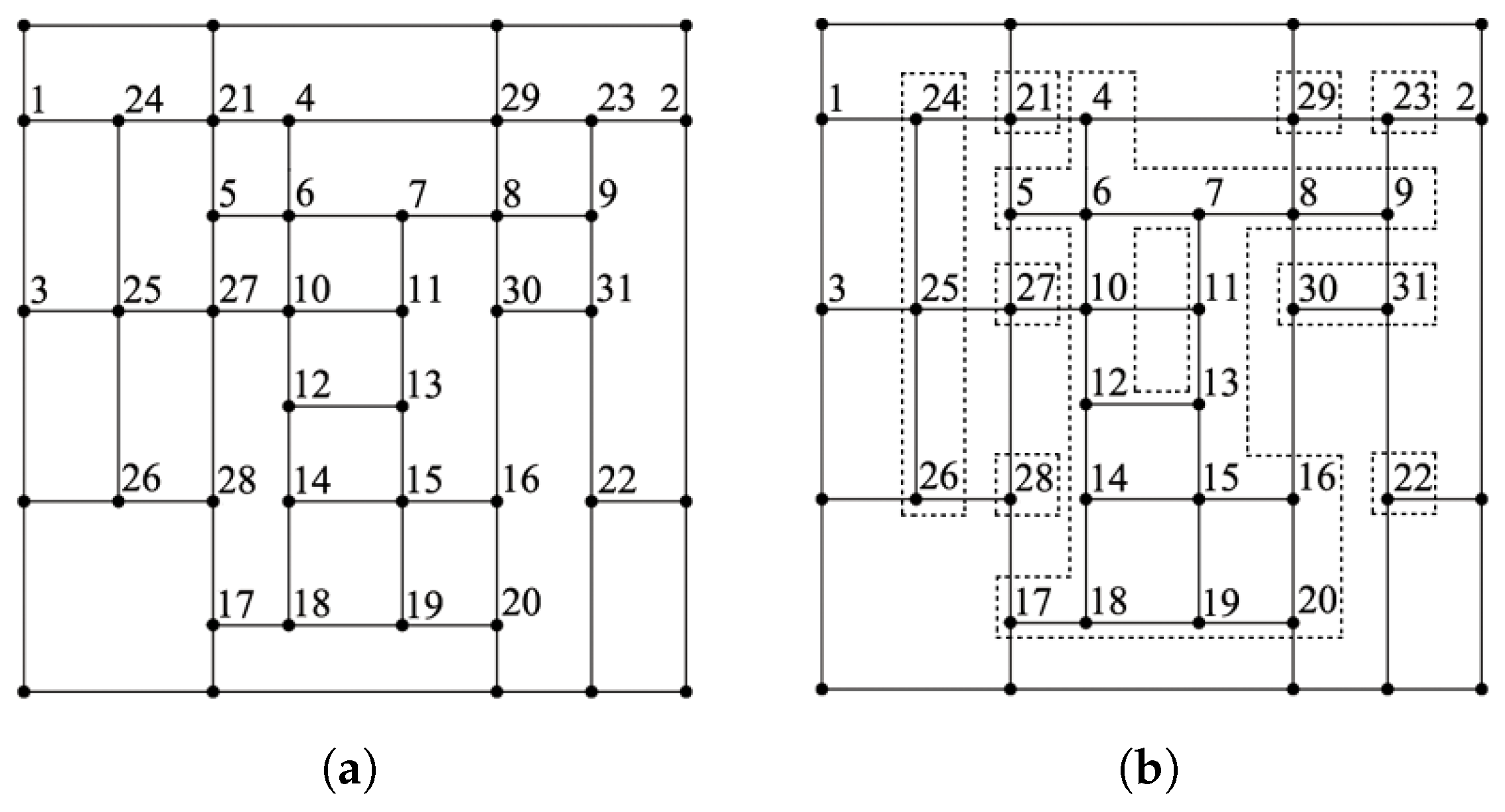
Figure 1. (a) A T-mesh. (b) Its T-connected components.
Mathematics 13 02886 g001
Figure 2. (a) The smoothing cofactors around v i , j . (b) The smoothing cofactors along a horizontal T-segment.
Mathematics 13 02886 g002
Figure 3. (a) A T-mesh T 1 containing a T-cycle (highlighted in red). (b) A T-mesh T N containing an N-nested T-cycle (highlighted in red).
Mathematics 13 02886 g003
Figure 4. (a) T-mesh T 1 (same as Figure 3a) with smoothness distribution r : smoothness 1 for blue interior segments and smoothness 2 for other interior segments (red and black). (b) The degeneration of T-mesh T 1 .
Mathematics 13 02886 g004
Figure 5. The two rings composed of alternating red and blue segments in T 1 .
Mathematics 13 02886 g005
Figure 6. (a) T-mesh T with smoothness distribution r : smoothness 1 for blue interior segments and smoothness 2 for other interior segments (red and black). (b) The degeneration of T-mesh T .
Mathematics 13 02886 g006
Figure 7. T-mesh T 2 containing a 2-nested T-cycle with smoothness distribution r : smoothness 1 for blue interior segments and smoothness 2 for other interior segments (red and black).
Mathematics 13 02886 g007
Figure 8. The degeneration of T-mesh T 2 : (a) both T-cycles are degenerate; (b) the inner T-cycle is degenerate (the remaining T-cycle is highlighted in red).
Mathematics 13 02886 g008
Figure 9. A T-mesh T 3 containing a 3-nested T-cycle with smoothness distribution r : smoothness 1 for blue interior segments and smoothness 2 for other interior segments (red and black).
Mathematics 13 02886 g009
Figure 10. The degeneration of T-mesh T 3 : (a) The T-cycles are completely degenerate. (b) The inner T-cycles T c 2 and T c 3 are degenerate(the remaining T-cycle is highlighted in red). (c) The innermost T-cycle T c 3 is degenerate(the remaining nested T-cycle is highlighted in red).
Mathematics 13 02886 g010
Disclaimer/Publisher’s Note: The statements, opinions and data contained in all publications are solely those of the individual author(s) and contributor(s) and not of MDPI and/or the editor(s). MDPI and/or the editor(s) disclaim responsibility for any injury to people or property resulting from any ideas, methods, instructions or products referred to in the content.