Abstract
This paper investigates the nonlinear dynamics of the wheel-side planetary reducer, considering the tooth wear effect. The tooth wear model based on the Archard adhesion wear theory is established, and the impact of tooth wear on meshing stiffness and piecewise-linear backlash of the planetary gear system is discussed. Then, the torsional vibration model and dimensionless differential equations considering tooth wear for the wheel-side planetary reducer are established, in which meshing excitations include time-varying mesh stiffness (TVMS), piecewise-linear backlash, and transmission error. The dynamic responses are numerically solved using the fourth-order Runge–Kutta method. On this basis, the nonlinear dynamics, such as the bifurcation and chaos properties of the wheel-side planetary reducer with tooth wear, are analyzed. Simulation results demonstrate that the existence of tooth wear reduces meshing stiffness and increases backlash. The reduction in the meshing stiffness changes the bifurcation path and chaotic amplitude of the system, inducing chaotic phenomena more easily. The increase in the gear backlash causes a higher amplitude of the relative displacement and more severe vibration.
MSC:
34C23; 37G15
1. Introduction
The imperative for sustainable transportation systems has driven the rapid global adoption of electric vehicles (EVs), recognized as a pivotal strategy for mitigating greenhouse gas emissions, reducing air pollution, and decreasing dependence on fossil fuels [1,2]. In-wheel motored driving (IWMD), a new method for driving vehicles, has been widely adopted by automotive companies, such as BYD, ZF, and Mercedes-Benz, due to its high energy transmission efficiency and flexible driving manner. By integrating the electric motor directly within or adjacent to the wheel hub, IWMD EVs eliminate the need for traditional central driveshafts, differentials, and associated power transmission losses [3,4]. A critical component enabling the compact and efficient design of IWMD EVs is the wheel-side planetary reducer. Positioned directly between the high-speed in-wheel motor and the wheel, this gearbox undertakes the essential task of torque amplification and speed reduction under demanding operational conditions [5]. Its compactness, high power density, load-sharing capabilities, and stable transmission make it an ideal choice for this application. The planetary gear reducer is composed of multiple meshing gear pairs. The dynamic excitations of different gear pairs (between the sun gear, ring gear, and planet gears) interact with each other, leading to complex vibration behaviors of the system [6,7].
Extensive research has been conducted on gear transmission systems, taking into account meshing nonlinear excitations. Based on the harmonic balance method, Sun et al. applied the discrete Fourier transformation (DFT) to planetary gear analysis and revealed the influence of internal dynamic excitations, such as multiple backlashes, time-varying mesh stiffness, etc., on gear transmission behaviors [8]. This study illustrates that nonlinear internal excitation affects the gear meshing force, and the TVMS is closely associated with gear failure [9,10]. To address the nonlinear vibration of planetary gears induced by TVMS, researchers typically employ the finite element method, energy method, and boundary element method to investigate the dynamic characteristics of the system [11,12]. Among them, the potential energy method based on the variable cross-section cantilever beam theory not only solves the problem of high-frequency vibration but also significantly reduces the computational burden. The method was employed by Liang et al. to evaluate the meshing stiffness of the planetary gear set [13]. The crack propagation model has also been developed and studied [14].
The nonlinear interactions between different gears within the planetary reducer are quite complex [15]. The high-speed motor in the planetary gear system affects the reliability of the transmission system in the in-wheel motored electric vehicle [16]. This results in various failure modes of the planetary gear tooth [17,18]. Tooth wear usually occurs in the early phase, thus affecting the transmission performance of the planetary gear [19,20]. Although the theory about gear fault diagnosis has been extensively studied [21,22], accurate prediction of gear failure is quite difficult due to the complex gear interaction behaviors. If gear failure is ignored and the dynamics analysis on the planetary gear focuses only on the healthy state, the results will deviate from the true values. As one of the earliest and most obvious forms of gear failure, tooth wear has a great effect on the system’s nonlinear dynamics. It is therefore necessary to establish a nonlinear dynamic model of the wheel-side planetary reducer for in-wheel motored electric vehicles that accounts for tooth wear. This model will serve as a basis for analyzing the system’s dynamic behavior in detail.
However, it is difficult to describe the type and degree of tooth surface faults accurately, such as pitting, wear, spalling, and cracks, making the modeling and dynamic characteristic analysis of the gear system extremely complex. Taking account of the Wigner-Ville distribution, Wang et al. compared the dynamic response of healthy planetary gears with the gear responses considering the pitting and crack defects, and pointed out that the meshing stiffness of faulty gears is smaller [23]. Among different kinds of gear failures, tooth wear is regarded as one of the most significant factors that affect the gear transmission vibration behaviors [24,25]. Kuang et al. established the gear dynamics equation considering the tooth wear and indicated that the tooth wear would change the tooth surface profile during the meshing process [26]. The spectrum diagram of the gear responses under various working conditions is analyzed by means of a numerical method. Variations in the operating state of the gear transmission (e.g., load fluctuations, speed adjustments) can also alter the system’s excitation frequency, damping ratio, and backlash, among other key parameters. Guo and Li et al. investigated the influence of gear backlash and damping coefficient on the dynamic characteristics of the planetary gear, and discussed the relationship between the system’s chaotic behaviors with these two parameters [27,28]. Sheng et al. studied the bifurcation, chaos, and nonlinear behavior of a planetary gear system qualitatively with different meshing frequencies, piecewise-linear backlash, and sun gear bearing clearance [29].
A review of existing studies on the modeling methods and nonlinear dynamics analysis of planetary gear transmissions for in-wheel motored electric vehicles reveals a critical gap: the changes in gear meshing induced by tooth wear are rarely considered in system modeling. This omission limits the accuracy of dynamic behavior descriptions. Therefore, this study introduces the gear tooth wear into the dynamic model of the planetary gear reducer, and the system’s nonlinear dynamics are further investigated. The main contribution of this study includes the following aspects: (1) The Archard adhesion wear theory is applied to establish the tooth wear model of the planetary gear reducer for an in-wheel motored electric vehicle. On this basis, the TVMS model based on the variable cross-section cantilever beam is built, and the impact of the tooth wear on the TVMS and piecewise-linear backlash is analyzed. (2) The bifurcation and chaotic characteristics of the planetary gear reducer under various excitation frequencies considering the tooth wear are studied, which provides a basis for the optimization of the system operation region.
Specifically, the rest of the paper is organized as follows: Section 2 establishes the dynamic model of the planetary reducer for the in-wheel motored electric vehicle. Section 3 calculates the tooth wear; on this basis, the TVMS and piecewise-linear backlash models with the tooth wear are built. Section 4 describes the dimensionless excitations and the differential equation of the planetary gear reducer. Numerical solutions are given in Section 5. The conclusions are summarized in Section 6.
2. Dynamic Model of the Wheel-Side Planetary Reducer System
The in-wheel electric vehicle wheel-side reducer studied in this paper can be simplified as consisting of an electric motor, a planetary gear set, and a wheel. Based on the lumped-parameter method, the torsional vibration dynamics model of the wheel-side reducer system is shown in Figure 1, where kms, kcw represent the torsional connection stiffness, and cms, ccw represent the torsional connection damping. The planetary gear set adopts a single-stage 2K-H type planetary gear set. It includes a sun gear (s), a ring gear (r), a planet carrier (c), and three planet gears (pj), where the subscript j (j = 1, 2, 3) denotes the j-th planet gear. The internal ring gear is rigidly fixed to the housing with zero rotational displacement. The lumped dynamics model of the single-stage planetary gear set is shown in Figure 2, which consists of three coordinate systems. The fixed coordinate system OXY is the common coordinate system of the planetary gear system. The rotating coordinate system oxy rotates with the planet carrier of the planetary gear set, the rotating coordinate system ojxjyj rotates with the j-th planet gear of the planetary gear system.
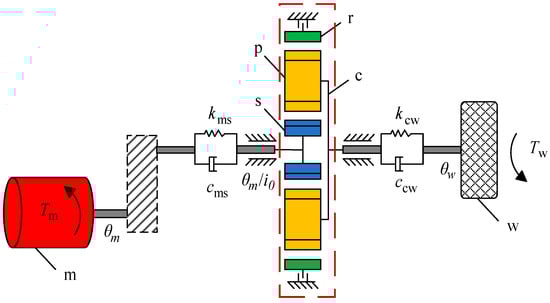
Figure 1.
Torsional vibration dynamics model of the wheel-side reducer system.
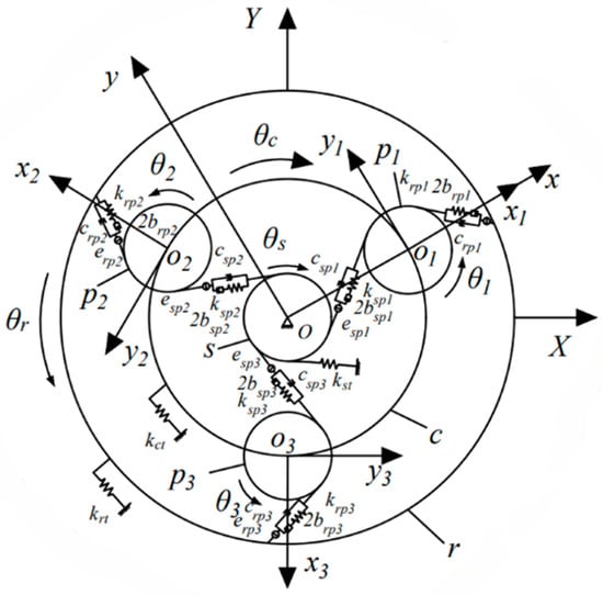
Figure 2.
Lumped dynamics model of the single-stage planetary gear set.
The mesh of the sun gear and ring gear with planetary gears is represented by a periodically time-varying stiffness element kspj and krpj, respectively. The backlash between gear teeth is described by a piecewise-linear backlash function f that includes a backlash of amplitude 2bspj and 2brpj. cspj and crpj are regarded as the meshing damping between the sun gear and planet gear, and the ring gear and planet gear, respectively. espj and erpj are the transmission errors within the sun–planet gear pair and the ring–planet gear pair, respectively. Tm and Tw are the motor torque and the wheel load torque, respectively. i0 is the ratio between the motor and wheel-side planetary reducer.
The lumped parameter method is used to develop the nonlinear dynamic model of the wheel-side planetary reducer system with the following assumptions [30,31].
- The planet carrier, ring gear, sun gear, and planet gears are regarded as rigid bodies.
- The meshing between different gears is simplified as cylinders connected by a spring and damping. Other connections are considered as an elastic spring.
- The planet gears on the planet carrier are equally distributed along the circumferential direction.
- The dispersed meshing force within the planetary reducer due to axial vibration is ignored.
The established dynamic differential equations include the axial torsional motion of eight degrees of freedom: the motor, the planetary carrier in the planetary gear set, the sun gear, the ring gear, three planetary gears, and the wheel. The generalized coordinate vector can be defined as [32]
where θm denotes the angle displacement of the motor model. θc, θs, and θr are the angle displacements of the planet carrier, sun gear, and ring gear of the planetary reducer, respectively. θpj denotes the angle displacement of the planet gears, and θw is the angle displacement of the wheel.
To more clearly demonstrate the relative vibrations between components and reduce the instability in the numerical solution of the equations caused by the rigid body angular displacements of multiple degrees of freedom, relative coordinates are introduced to convert the rigid body angular displacement θ into the relative displacement X along the gear meshing line direction, which can be expressed as:
According to Lagrange’s equation, the dynamic equations of the transmission system are derived as shown in Equation (3) [33]:
Some parameters in the equation are calculated as follows. Due to the influence of wear on the time-varying meshing stiffness and backlash, their calculations will be explained in detail later.
where Ii denotes the moment of inertia of each component, kespj and kerpj represent the average meshing stiffness of the internal and external meshing pairs in the planetary gear set, respectively. ξ denotes the meshing damping ratio of the system’s internal and external meshing pairs. The meshing damping ratio of each gear pair is assumed to be the same.
3. Dynamic Gear Mesh Excitation Considering Tooth Wear
In the planetary gear system, the wear of the sun gear and ring gear takes place on one side, while the planet gears undergo the alternating contact wear from the sun gear and the ring gear. The impact of tooth wear on the meshing stiffness and the piecewise-linear backlash is investigated in detail in this section.
3.1. Tooth Wear Calculation
Due to different relative sliding speeds on the meshing points between the two tooth surfaces, the actual tooth wear is non-uniformly distributed in the normal direction of the tooth profile under the action of the tooth surface contact stress. In this study, the Archard adhesion wear theory is employed to describe the wear depth [34].
where V denotes the volume of worn material. S denotes the sliding distance between the contacting surfaces. K denotes the dimensionless wear coefficient. W is the normal load, and H denotes the roughness of the tooth contact surface.
The Archard adhesion wear theory can also be converted into the wear depth of each point ‘p’ as [35]
where hp denotes the wear depth of point ‘p’, and C denotes the local contact pressure, the wear coefficient K is constant, the upper limit of integration Ls denotes the total sliding distance.
Combined with the relative sliding distance Sp at the meshing position, the wear depth of each tooth profile after n cycles of dynamic wear can be expressed as
where hp,n denotes the wear depth at point ‘p’ after n cycles of dynamic wear, hp,n−1 denotes the wear depth at the same point in the last contact cycle, and Cp,n−1 is the contact pressure of the last contact cycle at point ‘p’.
To depict the wear process of gear meshing, the contact behavior between the meshing point in the driving gear and the meshing point in the driven gear is described in Figure 3. The sliding distance at the contact point is determined based on the corresponding points and on the tooth surfaces of the driving gear and the driven gear during meshing. These two points can occupy three distinct positions from the start to the end of contact. The first position corresponds to the initial simultaneous contact of both points, as illustrated in Figure 3a. In the second position, the meshing point of the driven gear remains engaged, while the meshing point of the driving gear disengages, thereby generating a distance sp1 between the two selected points (Figure 3b). In the third position, when exits the meshing state, the distance between it and becomes , as shown in Figure 3c. According to the Hertzian contact theory, when the meshing point p1 in the driving gear moves along the contact line with a distance of , the meshing point in the driven gear will move with a distance of , and vice versa [36]. denotes the semi-Hertzian contact width and is calculated by
where ρ denotes the equivalent curvature radius of the contacting surface. E denotes the equivalent elasticity modulus of the material. Ft denotes the tangential force on the tooth surface and is given by
where M denotes the input torque acting on the driving gear. d0 denotes the pitch diameter. L1 denotes the tooth width of the driving gear.
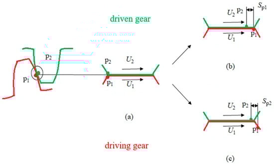
Figure 3.
Gear meshing process: (a) the meshing points and make contact, (b) the meshing point of the driving gear disengages, while the meshing point of the driven gear remains engaged, (c) the meshing point disengages.
The relative sliding distances and between the matching points and are [37]
where U1 and U2 are the peripheral velocities at the meshing point ‘’ and ‘’ and are described as
where d0 is the radius of the pitch circle. y1 and y2 denote the distance between the pitch point and meshing point of the meshing gears. ω1 and ω2 denote the corresponding angular velocities of different meshing gears. ϕ1 and ϕ2 are the pressure angles of the pitch circle for different meshing gears. y1, y2 can be expressed as
where R1 and R2 denote the radius of the base circle for the meshing gears. β1 and β2 denote the pressure angle at the meshing point ‘p’. By combining Equations (14) and (15), Equation (11) can be rewritten as
According to the Hertzian contact theory, the local contact pressure C is expressed as:
3.2. Tooth Wear Results
The planetary gear reducer of the in-wheel motored electric vehicle can be considered as multiple pairs of meshing between the driving and driven gears: the sun gear is the driving gear and the planet gear is the driven gear in the sun–planet gear meshing pair; the planet gear is the driving gear and the ring gear is the driven gear in the planet–ring gear meshing pair. In order to investigate the influence of different model parameters on the tooth wear, the meshing pair between the sun gear and the planet gear (sun–planet gear pair) is selected for numerical simulation analysis.
Figure 4 illustrates the wear depth distribution of the sun–planet gear pair under different meshing cycles, where Np denotes the meshing cycles of the driving gear. The smaller pressure angle represents that the meshing point is near the dedendum, and the larger pressure angle represents that the meshing point is near the addendum. Regarding the wear distribution between the dedendum and addendum, it can be seen from Figure 4 that the tooth wear depth generally decreases first and then increases with increasing pressure angle. When the pressure angle is 20°, the tooth wear depth is nearly zero. This is because the pressure angle at the pitch circle meshing point is 20°, where the circumferential speeds of the two meshing points and are equal. The relative sliding distance at meshing points for different pressure angles is shown in Figure 5. It can be seen that the sliding distance between the two meshing points is nearly zero at the pitch circle meshing point, and, therefore, the tooth wear is negligible. Furthermore, Figure 4 shows that the tooth wear depth is directly proportional to the number of meshing cycles. As the number of meshing cycles increases, the wear depth becomes more severe. When the meshing pressure angle is around 16° or 24°, sudden changes in tooth wear occur due to the alternation between single and double tooth meshing. The load distribution during the gear meshing process is shown in Figure 6, where segments AB and DE correspond to double-tooth meshing contact occurring at pressure angles outside the 16°–24° range, during which the load is shared by two tooth pairs. Segment BD corresponds to single-tooth meshing contact occurring at pressure angles within the 16°–24° range [25]. During single-tooth meshing, the load is borne by a single tooth pair, resulting in increased contact stress and consequently a significant increase in sliding distance, leading to more severe wear.
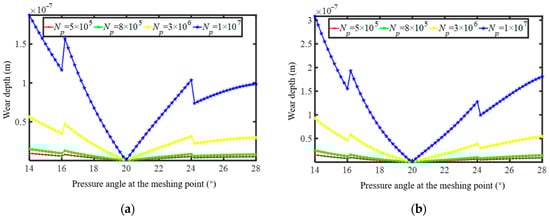
Figure 4.
Tooth wear depth in the sun−planet gear pair: (a) sun gear (b) planet gear.
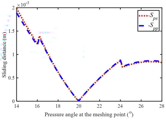
Figure 5.
Sliding distance of driving and driven gears in sun−planet gear.
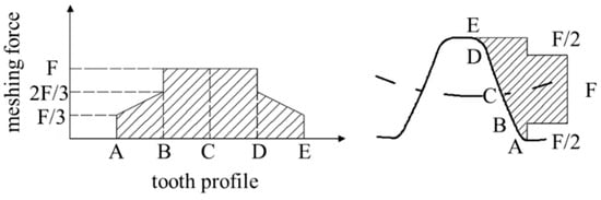
Figure 6.
Load distribution at each position of tooth profile.
3.3. TVMS Model with Tooth Surface Wear
The accumulation of tooth wear will change the tooth profile and reduce the tooth thickness to different degrees along the meshing position with the increase in the meshing cycles. The meshing stiffness of the planetary gear system, considering the aforementioned tooth wear, is obtained by utilizing the deformation theory of a variable cross-section cantilever beam. The meshing force considering the gear tooth is illustrated in Figure 7. Equations (23)–(25) describe the bending potential energy Ub, the shear potential energy Us, and the axial compressive potential energy Ua stored due to tooth deformation [38].
where α1 denotes the pressure angle at the meshing point. Fa and Fb are the transverse force and radial force at the meshing point. d is the lateral distance between the meshing point and the base circle. h denotes the longitudinal distance between the meshing point and the symmetry line of the tooth. The upper limit of the integral d−hpsinα1 represents the effective length of the cantilever beam after tooth wear. Ix and Ax denote the moment of inertia and the sectional area of the section at the meshing point. G denotes the shear modulus. The coefficient 1.2 in Equation (24) is an empirical correction factor for the distribution of shear stress on the cross-section of the tooth. The parameters Ix, Ax, and G can be calculated using the following equations [39]:
where Rb denotes the radius of the base circle. α2 is the half tooth radian of the base circle. hx denotes the distance between the meshing point and the symmetry line of the tooth. ν denotes the Poisson’s ratio, and L is the tooth width.
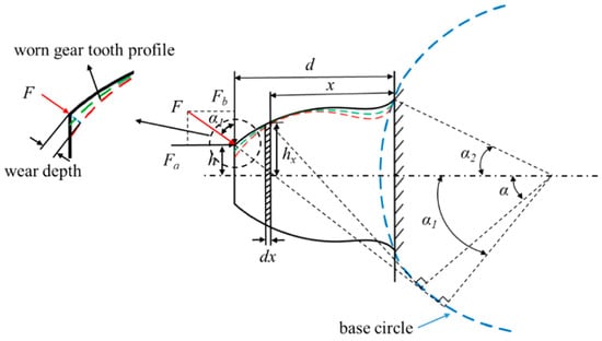
Figure 7.
Schematic diagram of the meshing force based on the beam model.
The single tooth meshing stiffness ks(α1) and the double tooth meshing stiffness kd(α1) are calculated by
where kh denotes the Hertzian contact stiffness. kb denotes the bending stiffness. ka and ks denote the axial compressive stiffness and the shear stiffness, respectively. kf is the deformation stiffness. These five types of stiffness can be derived as
where uf is the height from the meshing point to the dome point of the root circle. Sf is the arc length corresponding to the full tooth at the root circle. uf and Sf can be expressed by Equations (37) and (38). L*, M*, P*, and Q* are constants related to θf and hr, which can be obtained by the polynomial function as described by Equation (39) and the parameters in Table 1.
where hr denotes the ratio of the root circle radius to the shaft hole radius.

Table 1.
Stiffness coefficient of gear tooth matrix.
Figure 8 depicts the TVMS of the sun–planet meshing pair and the ring–planet meshing pair. The gear tooth has an impact on the TVMS of the planetary reducer. The tooth wear changes the tooth profile and reduces the tooth thickness, resulting in a decrease in the potential energy. In general, the tooth wear does not seem to have a significant impact on the TVMS in early wear. However, when excessive wear after billions of cycles of gear meshing happens, the TVMS decreases significantly. As shown by Figure 8, the TVMS in the planet–ring gear meshing pair is larger than that in the sun–planet gear meshing pair. The TVMS for the cases where there is no tooth wear and the tooth wear corresponding to 2 × 10¹¹ gear meshing cycles is nearly the same, while the TVMS is obviously reduced after 2 × 10¹² meshing cycles. Although tooth wear exerts no significant influence on TVMS in the early wear stage, it does affect the nonlinear dynamic behavior of the system. This effect will be discussed in detail in Section 5. Meanwhile, it can be seen from Figure 8 that the influence of the tooth wear on the double-tooth-pair meshing area is more significant than that on the single-tooth-pair meshing area, especially in the sun–planet gear meshing.
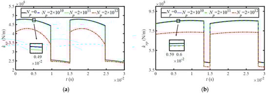
Figure 8.
The TVMS of the planetary reducer considering the tooth wear: (a) sun−planet gear (b) planet−ring gear.
3.4. Piecewise-Linear Backlash Model with Tooth Surface Wear
During the gear meshing process, a certain gap must be left between the tooth profiles to form the lubrication. The tooth backlash model is expressed by a piecewise-linear function, which can directly describe the nonlinear gear meshing characteristics. The tooth backlash function can be expressed as [28]
where xl denotes the relative meshing displacement. 2bl denotes the initial gear backlash, where the subscript l denotes spj or rpj. The total wear depth between meshing pairs is given by hp = hp1 + hp2, where hp represents the total wear depth of the meshing pair, hp1 denotes the wear depth of the driving gear, and hp2 denotes the wear depth of the driven gear.
Figure 9 depicts the backlash model of the planetary gear reducer considering the tooth wear, where the horizontal axis represents the relative meshing displacement between gears, and the vertical axis is expressed as tooth clearance. It can be seen that, with the increase in the gear rotational cycles, the backlash also increases due to the tooth wear factors. When the number of gear meshing cycles reaches a certain value, the backlash is remarkable.
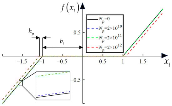
Figure 9.
Piecewise-linear backlash considering the tooth wear.
4. Nonlinear Dynamic Equation of the Planetary Gear Reducer
In order to analyze the nonlinear dynamics of the planetary gear reducer considering the tooth wear, the dimensionless equations that describe the dynamic model of the planetary gear system are established. Specifications of the planetary gear system are listed in Table 2.
Table 2.
Geometrical parameters of the planetary gear.
4.1. Dimensionless Excitations of the System
Since the ring gear of the gearset is mounted on the housing, according to the transmission dynamics of the planetary gear system, the meshing frequency can be derived as [40]
where and denote the rotational frequency of the sun gear and the carrier. Zs and Zr denote the teeth number of the sun gear and the ring gear, and denotes the meshing frequency.
A dimensionless time scale is introduced, and its calculation is given as
where kespj denotes the average meshing stiffness between the sun and planet gears. Md denotes the equivalent mass of the planetary gear set.
where Ms denotes the equivalent mass of the sun gear. Mce denotes the equivalent mass of the planet carrier. Mpj denotes the equivalent mass of the j-th planet gear.
Introducing the dimensionless displacement scale bd, the dimensional relative displacement , velocity , acceleration , dimensionless excitation frequency , and dimensionless backlash of the system can be expressed as
4.1.1. Dimensionless Time-Varying Meshing Stiffness
The time-varying meshing stiffness of the single and double tooth with alternating meshing during one meshing cycle is calculated as [41]
where θ1 denotes the wheel angle. ω is the wheel’s angular velocity. θd and θs are the wheel angles of double and single meshing areas, which satisfy the relationship as shown by Equation (46).
where Z1 denotes the tooth number of the driving gear.
The nonlinear TVMS can be represented as a rectangular wave with a certain time period. The Fourier series expansion of Equation (47) is used for the harmonic analysis, which includes the influence of gear tooth wear.
where keipj denotes the average amplitude, ku denotes the varying amplitude. φu denotes the initial phase angle.
4.1.2. Dimensional Periodic Transmission Error
The periodic transmission error function can be simplified as a sinusoidal function form as [42]
where Eipj and φipj (i = s, r) denote the amplitude and the initial phase angle of the comprehensive meshing error.
4.1.3. Dimensional Piecewise-Linear Backlash
The piecewise-linear backlash functions are defined as
where (l = spj, rpj) denotes the gear backlash, including the amount of gear tooth wear.
4.2. Dimensionless Differential Equation of the Planetary Gear Reducer
Based on the above equations, the non-dimensional motion differential equations of the HEV transmission system in the relative displacement coordinate system are derived as presented in Equation (50) [43].
4.3. Periodic Solutions of the System and Stability Judgment
Since the nonlinear dynamic model of the wheel-side planetary reducer established in this paper includes a piecewise-linear backlash function and time-varying mesh stiffness (TVMS), the system equations form a non-smooth dynamic system. It is difficult to directly obtain an explicit expression for its periodic solutions through analytical methods. This section introduces the pseudo-fixed point tracing method combined with Floquet stability theory to find the periodic solutions of the system under specific parameters and to judge their stability. The results are compared with the system’s dynamic response obtained by numerical integration using the fourth-order Runge–Kutta method, thereby verifying the correctness of the numerical solution.
4.3.1. Solving for Periodic Solutions
Considering the dimensionless dynamic equations of the system as a non-autonomous system, the pseudo-fixed point tracing method [44] is used to solve for the periodic solutions. This method is suitable for non-smooth systems and can track coexisting periodic solutions under different excitation periods. Equation (50) is rewritten as follows:
where , is the excitation period. Define the Poincaré section at time , and introduce the distance function:
where ϕ denotes the position at time t of the trajectory starting from point X at time . A pseudo-fixed point is defined as a point where reaches a local minimum. When t = mTex (m is a positive integer), if there exists X* such that , then X* is a periodic solution point of the system with period mTex.
The specific steps are as follows:
Solve the algebraic equations F(0, X) = 0 to obtain the initial pseudo-fixed point.
Gradually increase t with time step Δt, tracking the minimum points of .
Check whether the periodicity condition is satisfied at t = mTex. If satisfied, record the periodic solution.
When the dimensionless rotational speed is Ωm = 0.251, the zero solution of the algebraic equations F(0, X) = 0 corresponding to the dynamic system is calculated as X(0) = (17.587, 0, 1.173, 0, 1.256, 0, 9.784, 0), which serves as the initial pseudo-fixed point for the continuous tracing process of pseudo-fixed points. Following the specific steps of the pseudo-fixed point tracing method, the following two coexisting periodic fixed points are obtained:
Period-1 fixed point = (17.446, 0.097, 1.289, −0.068, 1.163, 0.053, 9.713, −1.734);
Period-2 fixed point = (17.427, −0.116, 1.205, −0.001, 1.151, 0.014, 9.682, −2.341);
Starting from these periodic fixed points and integrating over the respective periods, the phase diagrams of each periodic solution can be obtained, as shown in Figure 10. The red dots in the figure represent the periodic fixed points.
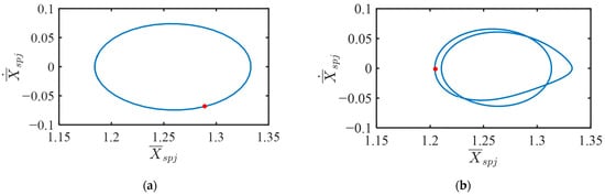
Figure 10.
Phase diagram when the excitation frequency (ξ = 0.05, = 1.5, = 1): (a) period-1, (b) period-2.
4.3.2. Stability Analysis of Periodic Solutions
For the obtained periodic solution X*(t), introduce a perturbation x(t) = X(t) − X*(t), resulting in the linearized system [45]:
where A(t) is the Jacobian matrix of the system at X*(t). Due to the non-smooth nature of the system, A(t) needs to be approximated using numerical differentiation methods.
According to Floquet theory, the stability of the periodic solution is determined by the magnitude of the eigenvalues (Floquet multipliers) of the state transition matrix B:
If the magnitudes of all Floquet multipliers are less than 1, the periodic solution is stable;
If there exists any Floquet multiplier with a magnitude greater than 1, the periodic solution is unstable;
If there exists a multiplier with a magnitude equal to 1, the system is in a critically stable state.
To find the state transition matrix B, numerically integrate the perturbation solutions for each column of the identity matrix across one full period. These solutions are then assembled to construct the matrix. The state transition matrices for the period-1 and period-2 solutions are solved as B1 and B2, respectively.
Further analysis of the maximum magnitude of the eigenvalues of these two matrices, i.e., the maximum magnitude of the Floquet multipliers, yields λ(B1) = 5.187 and λ(B2) = 0.896. Clearly, when Ωm = 0.251, only the period-2 solution is a stable motion pattern, while the period-1 solution is unstable. As verification, under the same set of parameters, the Runge–Kutta method is used for direct numerical integration over a long time period. After removing the transient response, the steady-state response of the system, expressed in time-domain diagrams and Poincaré maps, is shown in Figure 11.
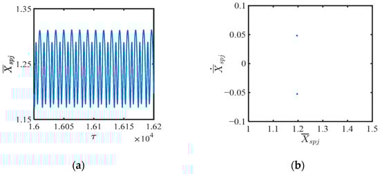
Figure 11.
The system’s dynamic response when the excitation frequency (ξ = 0.05, = 1.5, = 1): (a) Time history, (b) Poincaré map.
It can be observed that when Ωm = 0.251, the system exhibits a stable period-2 motion state, which is consistent with the analysis results obtained using the pseudo-fixed point tracing method combined with Floquet theory. The accuracy of the numerical integration method was verified, laying the foundation for subsequent global system response analysis.
5. Simulation Study of the System Dynamics
The nonlinear dynamic equations as shown by Equation (50) are solved by using the fixed-step fourth-order Runge–Kutta method [46]. The time step was chosen as a fraction of the meshing period (Tex/200) to accurately capture the high-frequency components. The configuration parameters are given in Table 3. The first 800 cycles of the system are omitted due to the transient response of the system. The bifurcation diagram of the system’s dynamic response with respect to the excitation frequency was obtained via the Poincaré section method [47]. The global bifurcation diagrams, time history diagrams, phase trajectories, and Poincaré maps are described to analyze the nonlinear dynamics of the system considering the tooth wear effect, and the maximum Lyapunov exponent (MLE) of the system was calculated using the Rosenstein algorithm [48].
Table 3.
Configuration parameters of the planetary gear system.
5.1. Dynamic Characteristics Without Tooth Wear
In order to highlight the impact of the tooth wear on the system’s nonlinear dynamics, different dimensionless relative displacements under various excitation frequencies for the unworn tooth are first calculated and analyzed, as shown in Figure 12. The meshing damping ratio ξ is 0.05. The amplitude of the dimensionless transmission error is 1.5 and the dimensionless backlash is 1. It can be seen from Figure 12 that the system dynamics are highly nonlinear under different excitation frequencies because of the strong coupling of the gear backlash, meshing error, and time-varying meshing stiffness. The system exhibits non-periodic motion under some excitation frequencies, and will experience multiple transitions from the periodic motion to chaotic motion with the change of excitation frequency. Although the chaotic amplitude of each relative displacement is different, the overall trend of the chaotic response is similar. That is, the chaotic motions of different components within the planetary gearset are motivated by the same frequency. When the excitation frequency is 0.181, 0.251, 0.346, 0.503, and 0.659, the system is bifurcated from a single point to several discrete points with uneven distribution, and the system dynamics transits from a periodic manner to an obviously chaotic manner.
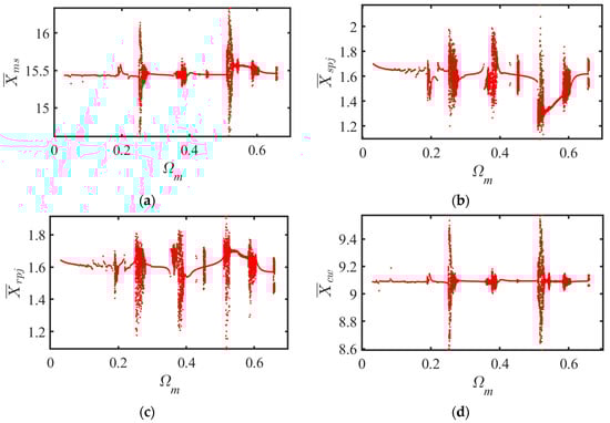
Figure 12.
Dimensionless displacement of lumped parameter model under different excitation frequency (ξ = 0.05, = 1.5, = 1): (a) dimensionless displacement ; (b) dimensionless displacement ; (c) dimensionless displacement ; (d) dimensionless displacement .
The maximum Lyapunov exponent of the system is shown in Figure 13. It can be observed that the Lyapunov exponent changes from negative to positive at the above-mentioned several excitation frequency points, which is consistent with the bifurcation characteristics. The similarity of the dynamic motion behavior within the planetary reducer depends on the configuration parameters. Therefore, in the following discussion, is selected to investigate the system dynamic behaviors considering the tooth wear.
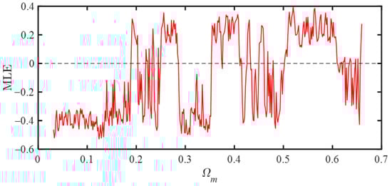
Figure 13.
The maximum Lyapunov exponent diagram under different excitation frequencies (ξ = 0.05, = 1.5, = 1).
Figure 14, Figure 15 and Figure 16 describe the responses of without tooth wear. As illustrated by Figure 14, the system exhibits periodic motion when Ωm ≤ 0.251. Specifically, when the excitation frequency Ωm is 0.251, the system settles into a stable limit cycle, exhibiting periodic motion. The time history in Figure 14a demonstrates that the periodic motion includes two kinds of periodic curves. The phase trajectory shown in Figure 14b forms a closed orbit, confirming a stable limit cycle of period-2. The discrete points in the Poincaré map (Figure 14c) further confirm the existence of a stable limit cycle, as the system state asymptotically converges to a periodic solution independent of initial conditions. The chaotic motion of the system for a certain frequency, for example, when the frequency Ωm is 0.534, is shown in Figure 15. The time history response in Figure 15a gives irregular fluctuations from cycle to cycle. The phase trajectories in Figure 15b are highly disordered and spread almost throughout the entire phase area, which indicates the chaotic motion. The strange attractor of the chaotic motion is illustrated in the Poincaré map as shown in Figure 15c. The system will also experience the three quasi-periodic motions for a certain frequency, for example, when the excitation frequency Ωm is 0.628, as shown in Figure 16. The phase trajectories in Figure 16b repeat for every three periods but also show differences between each other. There are three closed loops in the Poincaré map in Figure 16c. Based on the global bifurcation diagrams, it can be concluded that most of the system dynamics are in 2T-periodic motion, 3T-quasi-periodic motion, and chaotic motion. Since there are several frequency points from periodic motion to chaotic motion, it is particularly important to determine the periodic motion range of the system. The dynamic behaviors of the planetary reducer are very sensitive to the excitation frequency Ωm, which can be used as a bifurcation parameter to examine the nonlinear dynamics.
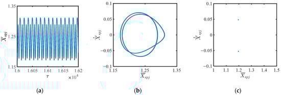
Figure 14.
The responses of without tooth wear when the excitation frequency is 0.251 (ξ = 0.05, = 1.5, = 1): (a) time history; (b) phase trajectories; (c) Poincaré map.
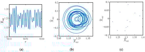
Figure 15.
The responses of without tooth wear when the excitation frequency is 0.534 (ξ = 0.05, = 1.5, = 1): (a) time history; (b) phase trajectories; (c) Poincaré map.
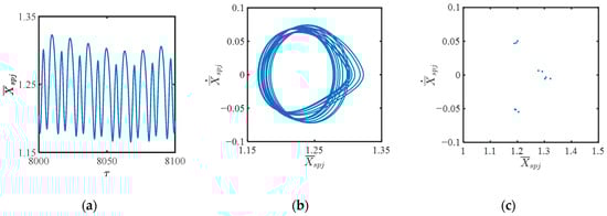
Figure 16.
The responses of without tooth wear when the excitation frequency is 0.628 (ξ = 0.05, = 1.5, = 1): (a) time history; (b) phase trajectories; (c) Poincaré map.
5.2. Dynamic Characteristics with Tooth Wear
As shown by the aforementioned analysis, the tooth wear will reduce the meshing stiffness and increase the piecewise-linear backlash, which will further affect the dynamic characteristics of the system. Taking the relative displacement between the sun and planetary gears with different meshing cycles as the research object, a partial bifurcation diagram is obtained and shown in Figure 17. It can be seen that as the meshing cycle increases, the amplitude of the relative displacement of the chaotic motion also increases. The excitation frequency when the system enters and exits the chaotic motion becomes smaller. This change can be more clearly observed through the maximum Lyapunov exponent graph in Figure 18. In order to better illustrate the impact of the tooth wear on the system dynamics, the following sections discuss the nonlinear dynamic characteristics of the system with different meshing stiffness and piecewise-linear backlash caused by the tooth wear.
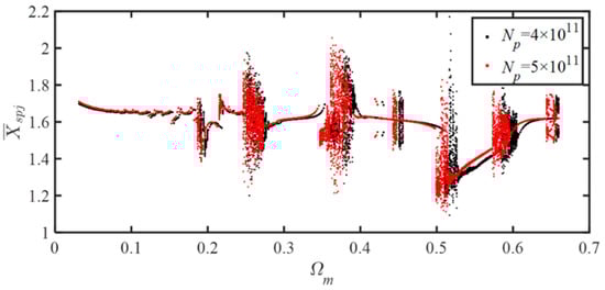
Figure 17.
Relative displacement bifurcation diagram of sun−planetary gears under different meshing times (ξ = 0.05, = 1.5).
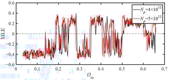
Figure 18.
The maximum Lyapunov exponent diagram under different meshing times (ξ = 0.05, = 1.5).
5.2.1. Influence of Meshing Stiffness
Due to the tooth wear, the meshing stiffness between the gear pairs will decrease with the increase in the wear depth. Table 4 lists the average meshing stiffness of different gear meshing pairs for four cases.
Table 4.
Meshing stiffness values under different meshing times.
Figure 19 describes the bifurcation diagram of with different kespj and kerpj. As shown by the figure, the reduction in the meshing stiffness will increase the amplitude of the chaotic period at a higher value of dimensionless excitation frequency. However, the magnitude of the relative motion in the quasi-periodic cycle remains nearly the same. When the dimensionless excitation frequency is less than 0.251, the amplitude of the relative motion does not change. Moreover, the path and timing of the transition from the periodic motion to chaotic motion are the same in four different cases, all of which exhibit chaos in the form of inverted bifurcation. When the dimensionless excitation frequency is greater than 0.251, the timing of the system entering the chaotic motion is changed. The smaller the meshing stiffness is, the longer the chaotic period and the larger the amplitude of the system chaos will be. At higher excitation frequencies, the chaotic amplitude will increase significantly. In addition, as shown by Figure 19d, when the meshing stiffness is lower than a certain value, the system fails to jump out of the chaotic motion at high excitation frequencies, and infinite chaos will occur, resulting in remarkable negative vibration influences on the system.
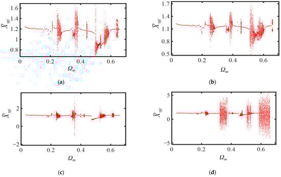
Figure 19.
Bifurcation diagrams for versus with different kespj and kerpj: (a) case1; (b) case2; (c) case3; (d) case4.
Furthermore, the dimensionless excitation frequency Ωm = 0.251 is selected as a case. Figure 20 depicts the time history, phase trajectories and Poincaré map of under different tooth wear degrees, which correspond to different meshing stiffness. It can be seen from Figure 20 that the amplitude of the relative vibration displacement for the unworn gear is obviously the smallest. With the increase in the tooth wear, the vibration amplitude increases significantly, and the chaos is characterized by more obvious irregular fluctuations from cycle to cycle, which can be illustrated by Figure 20b,c. As shown by the figures, when the tooth wear is relatively small, the phase trajectory demonstrates two close rings and the Poincaré map shows two discrete single points. The system moves in a 2T-periodic motion. When the wear depth increases, the system transits from the periodic motion to the chaotic motion under the dimensionless excitation frequency Ωm = 0.251. The phase trajectories in Figure 20b are highly disordered and spread almost throughout the entire phase area, with deep wear of the planetary gear system. It can be concluded that the reduction in the gear meshing stiffness caused by the tooth wear will affect the nonlinear dynamic characteristics of the planetary gear transmission system significantly. The decrease in the gear meshing stiffness will induce the chaotic motion at lower excitation frequencies and wider frequency domains. The chaotic motion happens more easily, caused by more serious tooth wear.
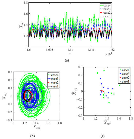
Figure 20.
under different wear degrees when the dimensionless excitation frequency = 0.251: (a) time history; (b) phase trajectories; (c) Poincaré map.
5.2.2. Influence of Piecewise-Linear Backlash
The tooth wear will increase the backlash between the two meshing gear pairs. Table 5 lists the backlashes of the gear meshing pairs in four different scenarios. Figure 21 compares the bifurcation diagrams and the MLE diagrams for versus Ωm and the corresponding phase trajectory diagram. It can be seen that the increase in the piecewise-linear backlash will increase the amplitude of the relative motion. The increase in backlash primarily acts to modulate the amplitude of the limit cycles present in the system. A larger backlash allows for greater free travel before tooth contact, enabling the gears to build more momentum and resulting in more intense impacts and consequently higher amplitude oscillations. However, the change in the gear backlash does not affect the bifurcation and chaotic characteristics of the system; that is, the excitation frequency that induces the system’s chaotic motion is regardless of the gear backlash. This suggests that for the parameter range studied, the backlash magnitude is not the primary bifurcation parameter governing the onset of chaos, but it is a critical parameter determining the energy and amplitude of the sustained limit cycle oscillations once they are established. Even so, the influence of the backlash caused by the tooth wear on the vibration amplitude cannot be ignored.
Table 5.
Different levels of backlash.
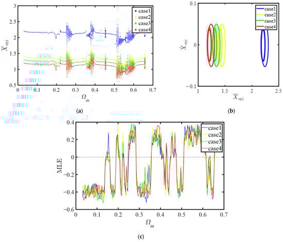
Figure 21.
System dynamic response under different backlash values: (a) bifurcation diagram; (b) phase trajectories; (c) the maximum Lyapunov exponent diagram.
6. Conclusions
This study investigates the nonlinear dynamics of the planetary gear reducer with tooth wear, which is applied in the in-wheel motored electric vehicle. The Archard adhesive wear theory is utilized to develop the tooth wear model and study the impact of meshing cycles on the wear condition. The meshing stiffness within the gear system, considering tooth wear, is obtained based on the deformation theory of a variable cross-section cantilever beam. The piecewise-linear backlash model with tooth wear is built. On this basis, dimensionless equations of the system model are formulated and solved by using the fourth-order Runge–Kutta method.
Simulation results show that tooth wear reduces meshing stiffness and increases piecewise-linear backlash. Specifically, tooth wear has a more significant impact on the meshing stiffness during double-tooth meshing than during single-tooth meshing. After hundreds of millions of meshing cycles, the meshing stiffness decreases significantly. Variations in gear meshing stiffness notably alter the system’s motion bifurcation path and chaotic amplitude: when meshing stiffness is low, periodic motion disappears, and global chaos occurs under high excitation frequencies. In contrast, an increase in gear backlash does not change the excitation frequency that triggers system bifurcation and chaos, but it gradually enhances the amplitude of relative motion. These findings provide a solid theoretical foundation for the optimal design and control of planetary gear reducers used in in-wheel motored electric vehicles.
Author Contributions
Conceptualization, D.S. and S.W.; methodology, D.S., Q.Z. and L.S.; software, D.S. and L.S.; validation, C.Y. and C.L.; data curation, D.S., Q.Z. and L.S.; writing—original draft preparation, D.S.; writing—review and editing, S.W. and K.Z.; project administration, S.W.; funding acquisition, S.W. All authors have read and agreed to the published version of the manuscript.
Funding
This research was funded by the National Natural Science Foundation of China (Grant No. 52272368), the Open Fund of State Key Laboratory of Mechanical Transmission (No. SKLMT-MSKFKT-202423), and the Special Fund Project for Basic Research of Zhenjiang city (JC2004006).
Data Availability Statement
The raw data supporting the conclusions of this article will be made available by the authors upon reasonable request.
Conflicts of Interest
Author Chun Li was employed by the company Higer Bus Company Limited. The remaining authors declare that the research was conducted in the absence of any commercial or financial relationships that could be construed as a potential conflict of interest.
References
- Shi, D.S.L.; Xu, H.; Wang, S.; Wang, L. Design and test of adaptive energy management strategy for plug-in hybrid electric vehicle considering traffic information. Energy 2025, 325, 136093. [Google Scholar] [CrossRef]
- Zhu, Z.; Zeng, L.X.; Chen, L.; Zou, R.; Cai, Y.F. Fuzzy Adaptive Energy Management Strategy for a Hybrid Agricultural Tractor Equipped with HMCVT. Agriculture 2022, 12, 1986. [Google Scholar] [CrossRef]
- Tong, Y.; Li, C.; Wang, G.; Jing, H. Integrated Path-Following and Fault-Tolerant Control for Four-Wheel Independent-Driving Electric Vehicles. Automot. Innov. 2022, 5, 311–323. [Google Scholar] [CrossRef]
- Li, Y.M.; Liu, Y.B.; Ji, K.Z.; Zhu, R.H. A Fault Diagnosis Method for a Differential Inverse Gearbox of a Crawler Combine Harvester Based on Order Analysis. Agriculture 2022, 12, 1300. [Google Scholar] [CrossRef]
- Zhu, Z.H.; Chai, X.Y.; Xu, L.Z.; Quan, L.; Yuan, C.C.; Tian, S.C. Design and performance of a distributed electric drive system for a series hybrid electric combine harvester. Biosyst. Eng. 2023, 236, 160–174. [Google Scholar] [CrossRef]
- Wang, W.; Durack, J.M.; Durack, M.J.; Zhang, J.; Zhao, P. Automotive Traction Drive Speed Reducer Efficiency Testing. Automot. Innov. 2021, 4, 81–92. [Google Scholar] [CrossRef]
- Gao, Y.Y.; Yang, Y.F.; Fu, S.; Feng, K.Y.; Han, X.; Hu, Y.Y.; Zhu, Q.Z.; Wei, X.H. Analysis of Vibration Characteristics of Tractor-Rotary Cultivator Combination Based on Time Domain and Frequency Domain. Agriculture 2024, 14, 1139. [Google Scholar] [CrossRef]
- Sun, T.; Hu, H. Nonlinear dynamics of a planetary gear system with multiple clearances. Mech. Mach. Theory 2003, 38, 1371–1390. [Google Scholar] [CrossRef]
- Benguria, R.D.; Depassier, M.C. Upper and lower bounds for the speed of fronts of the reaction diffusion equation with Stefan boundary conditions. Nonlinearity 2023, 36, 4425. [Google Scholar] [CrossRef]
- Winkler, M. Stabilization despite pervasive strong cross-degeneracies in a nonlinear diffusion model for migration-consumption interaction. Nonlinearity 2023, 36, 4438–4469. [Google Scholar] [CrossRef]
- Ericson, T.M.; Parker, R.G. Experimental measurement and finite element simulation of elastic-body vibration in planetary gears. Mech. Mach. Theory 2021, 160, 23. [Google Scholar] [CrossRef]
- Dai, H.; Long, X.; Chen, F.; Xun, C. An improved analytical model for gear mesh stiffness calculation. Mech. Mach. Theory 2021, 159, 104262. [Google Scholar] [CrossRef]
- Liang, X.; Zuo, M.J.; Patel, T.H. Evaluating the time-varying mesh stiffness of a planetary gear set using the potential energy method. Proc. Inst. Mech. Eng. Part C J. Mech. Eng. Sci. 2014, 228, 535–547. [Google Scholar] [CrossRef]
- Liang, X.; Zuo, M.J.; Pandey, M. Analytically evaluating the influence of crack on the mesh stiffness of a planetary gear set. Mech. Mach. Theory 2014, 76, 20–38. [Google Scholar] [CrossRef]
- Liu, C.; Yin, X.; Liao, Y.; Yi, Y.; Qin, D. Hybrid dynamic modeling and analysis of the electric vehicle planetary gear system. Mech. Mach. Theory 2020, 150, 103860. [Google Scholar] [CrossRef]
- Liu, Y.; Chen, L.; Cai, T.; Sun, W.; Xu, X.; Wang, S. Dual-pump control algorithm of two-speed powershift transmissions in electric vehicles. Automot. Innov. 2022, 5, 57–69. [Google Scholar] [CrossRef]
- Chaari, F.; Fakhfakh, T.; Haddar, M. Dynamic analysis of a planetary gear failure caused by tooth pitting cracking. J. Fail. Anal. Prev. 2006, 6, 73–78. [Google Scholar] [CrossRef]
- Feng, W.; Feng, Z.; Mao, L. Failure analysis of a secondary driving helical gear in transmission of electric vehicle. Eng. Fail. Anal. 2020, 117, 104934. [Google Scholar] [CrossRef]
- Wang, F.; Zhang, J.; Xu, X.; Cai, Y.; Zhou, Z.; Sun, X. New teeth surface and back (TSB) modification method for transient torsional vibration suppression of planetary gear powertrain for an electric vehicle. Mech. Mach. Theory 2019, 140, 520–537. [Google Scholar] [CrossRef]
- Sharma, V.; Parey, A. A review of gear fault diagnosis using various condition indicators. Procedia Eng. 2016, 144, 253–263. [Google Scholar] [CrossRef]
- Gołębski, R.; Szarek, A. Diagnosis of the operational gear wheel wear. Teh. Vjesn. 2019, 26, 658–661. [Google Scholar] [CrossRef]
- Zhang, R.; Gu, F.; Mansaf, H.; Wang, T.; Ball, A.D. Gear wear monitoring by modulation signal bispectrum based on motor current signal analysis. Mech. Syst. Signal Process. 2017, 94, 202–213. [Google Scholar] [CrossRef]
- Wang, F.; Cai, Q.; Zhang, Y. Failure analysis and wear mechanism study of a heavily loaded gear. Tribol. Int. 1985, 18, 93–99. [Google Scholar] [CrossRef]
- Choy, F.; Polyshchuk, V.; Zakrajsek, J.; Handschuh, R.; Townsend, D. Analysis of the effects of surface pitting and wear on the vibrations of a gear transmission system. Tribol. Int. 1994, 29, 77–83. [Google Scholar] [CrossRef]
- İmrek, H.; Düzcükoğlu, H. Relation between wear and tooth width modification in spur gears. Wear 2007, 262, 390–394. [Google Scholar] [CrossRef]
- Kuang, J.; Lin, A. The effect of tooth wear on the vibration spectrum of a spur gear pair. J. Vib. Acoust. 2001, 123, 311–317. [Google Scholar] [CrossRef]
- Guo, Y.; Parker, R.G. Dynamic analysis of planetary gears with bearing clearance. J. Comput. Nonlinear Dyn. 2012, 7. [Google Scholar] [CrossRef]
- Li, S.; Wu, Q.; Zhang, Z. Bifurcation and chaos analysis of multistage planetary gear train. Nonlinear Dyn. 2014, 75, 217–233. [Google Scholar] [CrossRef]
- Sheng, D.-p.; Zhu, R.-p.; Jin, G.-h.; Lu, F.-x.; Bao, H.-y. Bifurcation chaos study on transverse-torsional coupled 2K-Hplanetary gear train with multiple clearances. J. Cent. South Univ. 2016, 23, 86–101. [Google Scholar] [CrossRef]
- Zhang, J.; Guo, H.; Yu, H.; Zhang, T. Numerical experimental investigation on nonlinear dynamic characteristics of planetary gear train. J. Theor. Appl. Mech. 2020, 58, 1009–1022. [Google Scholar] [CrossRef]
- Yang, H.; Li, X.; Xu, J.; Yang, Z.; Chen, R. Dynamic characteristics analysis of planetary gear system with internal and external excitation under turbulent wind load. Sci. Prog. 2021, 104, 1–21. [Google Scholar] [CrossRef]
- Wang, F.; Xia, J.; Xu, X.; Cai, Y.; Zhou, Z.; Sun, X. New clutch oil-pressure establishing method design of PHEVs during mode transition process for transient torsional vibration suppression of planetary power-split system. Mech. Mach. Theory 2020, 148, 103801. [Google Scholar] [CrossRef]
- Liu, H.; Xie, Y.; Wu, Y.; Gao, P.; Han, L.; Xiang, C.; Ma, Y.; Yan, K.; Yan, Q.; Gai, J.; et al. Study on electromechanical coupling inherent vibration characteristics and parameter influencing law of EMT system used in HEV. Proc. Inst. Mech. Eng. Part D J. Automob. Eng. 2023. [Google Scholar] [CrossRef]
- Feng, K.; Smith, W.A.; Peng, Z. Use of an improved vibration-based updating methodology for gear wear prediction. Eng. Fail. Anal. 2021, 120, 9. [Google Scholar] [CrossRef]
- Anders Flodin, S.A. Simulation of mild wear in spur gears. Wear 1997, 207, 16–23. [Google Scholar] [CrossRef]
- Tunalioğlu, M.Ş.; Tuç, B. Theoretical and experimental investigation of wear in internal gears. Wear 2014, 309, 208–215. [Google Scholar] [CrossRef]
- Shen, Z.; Qiao, B.; Yang, L.; Luo, W.; Chen, X. Evaluating the influence of tooth surface wear on TVMS of planetary gear set. Mech. Mach. Theory 2019, 136, 206–223. [Google Scholar] [CrossRef]
- Wang, Y.A.; Wang, H.; Li, K.Y.; Qiao, B.J.; Shen, Z.X.; Chen, X.F. An analytical method to calculate the time-varying mesh stiffness of spiral bevel gears with cracks. Mech. Mach. Theory 2023, 188, 28. [Google Scholar] [CrossRef]
- Liang, X.; Zhang, H.; Liu, L.; Zuo, M.J. The influence of tooth pitting on the mesh stiffness of a pair of external spur gears. Mech. Mach. Theory 2016, 106, 1–15. [Google Scholar] [CrossRef]
- Parker, R.G. A physical explanation for the effectiveness of planet phasing to suppress planetary gear vibration. J. Sound Vib. 2000, 236, 561–573. [Google Scholar] [CrossRef]
- Chaari, F.; Fakhfakh, T.; Haddar, M. Analytical modelling of spur gear tooth crack influence on gearmesh stiffness. Eur. J. Mech. A-Solids 2009, 28, 461–468. [Google Scholar] [CrossRef]
- Ren, Z.-H.; Fu, L.; Liu, Y.-J.; Zhou, S.-H.; Wen, B.-C. Nonlinear Dynamic Characteristic Analysis of Planetary Gear Transmission System for the Wind Turbine. J. Appl. Nonlinear Dyn. 2015, 4, 281–294. [Google Scholar] [CrossRef]
- Wang, X. A Study on Coupling Faults’ Characteristics of Fixed-Axis Gear Crack and Planetary Gear Wear. Shock Vib. 2018, 2018, 4692796. [Google Scholar] [CrossRef]
- Li, T.J.; Zhu, R.P. Global Analysis of a Planetary Gear Train. Shock Vib. 2014, 2014, 6. [Google Scholar] [CrossRef]
- Li, T.J.; Zhu, R.P.; Bao, H.Y.; Xiang, C.L. Stability of motion state and bifurcation properties of planetary gear train. J. Cent. South Univ. 2012, 19, 1543–1547. [Google Scholar] [CrossRef]
- Shuai, M.; Zhang, Y.X.; Song, Y.L.; Song, W.H.; Huang, Y.S. Nonlinear vibration and primary resonance analysis of non-orthogonal face gear-rotor-bearing system. Nonlinear Dyn. 2022, 108, 3367–3389. [Google Scholar] [CrossRef]
- Zhang, X.; Zhong, J.X.; Li, W.; Bocian, M. Nonlinear dynamic analysis of high-speed gear pair with wear fault and tooth contact temperature for a wind turbine gearbox. Mech. Mach. Theory 2022, 173, 20. [Google Scholar] [CrossRef]
- Wang, J.; Chen, X.; Bi, X.C.; Luo, Z.J.; Mo, R.N. Dynamic analysis of TBM multi-gear parallel transmission system considering the influence of multiple factors. J. Mech. Sci. Technol. 2024, 38, 5323–5340. [Google Scholar] [CrossRef]
Disclaimer/Publisher’s Note: The statements, opinions and data contained in all publications are solely those of the individual author(s) and contributor(s) and not of MDPI and/or the editor(s). MDPI and/or the editor(s) disclaim responsibility for any injury to people or property resulting from any ideas, methods, instructions or products referred to in the content. |
© 2025 by the authors. Licensee MDPI, Basel, Switzerland. This article is an open access article distributed under the terms and conditions of the Creative Commons Attribution (CC BY) license (https://creativecommons.org/licenses/by/4.0/).