Abstract
Balancing efficiency and accuracy is often challenging in the numerical solution of three-dimensional (3D) point source acoustic wave equations for layered media. To overcome this, an efficient solution method in the spatial-wavenumber domain is proposed, utilizing the Non-Uniform Fast Fourier Transform (NUFFT) to achieve arbitrary non-uniform sampling. By performing a two-dimensional (2D) Fourier transform on the 3D acoustic wave equation in the horizontal direction, the 3D equation is transformed into a one-dimensional (1D) space-wavenumber-domain ordinary differential equation, effectively simplifying significant 3D problems into one-dimensional problems and significantly reducing the demand for memory. The one-dimensional finite-element method is applied to solve the boundary value problem, resulting in a pentadiagonal system of equations. The Thomas algorithm then efficiently solves the system, yielding the layered wavefield distribution in the space-wavenumber domain. Finally, the wavefield distribution in the spatial domain is reconstructed through a 2D inverse Fourier transform. The correctness of the algorithm was verified by comparing it with the finite-element method. The analysis of the half-space model shows that this method can accurately calculate the wavefield distribution in the air layer considering the air layer while exhibiting high efficiency and computational stability in ultra-large-scale models. The three-layer medium model test further verified the adaptability and accuracy of the algorithm in calculating the distribution of acoustic waves in layered media. Through a sensitivity analysis, it is shown that the denser the mesh node partitioning, the higher the medium velocity, and the lower the point source frequency, the higher the accuracy of the algorithm. An algorithm efficiency analysis shows that this method has extremely low memory usage and high computational efficiency and can quickly solve large-scale models even on personal computers. Compared with traditional FEM, the algorithm has much higher advantages in terms of memory usage and efficiency. This method provides a new approach to the numerical solution of partial differential equations. It lays an essential foundation for background field calculation in the scattering seismic numerical simulation and full-waveform inversion of acoustic waves, with strong theoretical significance and practical application value.
MSC:
35Q86
1. Introduction
The propagation of seismic waves plays a crucial role in various fields, including seismology, petroleum exploration, and subsurface imaging. In layered media, variations in properties such as wave velocity and density across different layers result in highly non-uniform wave propagation. These complexities make it challenging for traditional analytical methods to effectively address the propagation characteristics in such intricate media [1,2,3]. As a result, numerical simulation based on wave equations has become the primary tool for investigating acoustic wavefields in layered media [4,5,6,7]. These numerical simulation methods are significant in improving the accuracy and computational efficiency of wavefield simulation and play a key role in solving partial differential equations. At the same time, numerical methods provide efficient tools and methods for solving background fields in scattered wavefield calculations, greatly promoting technological progress in fields such as seismic exploration, resource exploration, and geophysical exploration.
Analytical methods, such as the wave function expansion method, multipole coordinate method, separation of variables, complex function method, and matching method, were widely used in the early studies of seismic wave propagation [2,5,8,9,10,11,12,13,14,15,16]. These methods usually have high accuracy and small computational complexity, but their application scope is mainly limited to simple models [3,17,18,19,20]. In practical applications, analytical methods require significant model simplifications, and the wavefield construction must strictly satisfy the wave equation and boundary conditions. Therefore, these methods meet considerable difficulties in solving practical problems.
Although layered media are often regarded as one-dimensional structures, most wavefields excited by seismic sources are three-dimensional elastic wavefields. Existing studies on the fundamental solutions in layered media primarily focus on 2D wavefields, with the few three-dimensional studies typically assuming cylindrical axisymmetry. However, even for simple layered models, the computation of three-dimensional wavefields faces challenges such as numerical implementation difficulties, complex computational processes, and limited flexibility, which restrict their application. As a result, the advantages of numerical methods for solving wavefields in layered media have become increasingly evident. Alterman et al. (1968) successfully applied the finite-difference method to the numerical simulation of elastic wave equations in horizontal layered media for the first time [21]. Jafar Gandomi and Takenaka (2007) developed a Finite-Difference Time Domain (FDTD) algorithm to calculate the plane wave response of a 1D attenuated Earth model by solving the seismic P-SV (2C) wave equation in the τ-p domain, which can obtain the seismic response of vertically non-uniform attenuated media [22]. After this work, Jafar Gandomi and Takenaka (2013) further extended the algorithm to solve the 3C (P-wave, SV wave, and SH wave) wave equation [23]. Sheikhhassani and Dravinski (2016) used the boundary element method to investigate the scattering of plane SH waves by multi-layered sites containing inclusions [24]. Liu Siqin et al. (2021) used the discrete complex image method and the double exponential rule to calculate Green’s function of layered seismic fields quickly, achieving the calculation of point source acoustic wavefields in layered media [4]. Edith Sotelo et al. (2021) applied the generalized finite-element method (GFEM) to simulate the acoustic wave equation in exploration seismology, evaluated its accuracy and efficiency by comparing it to the spectral-element method (SEM), and demonstrated that GFEM offers comparable performance, with advantages in handling unstructured grids and complex models [25]. Lei Wen et al. (2023) developed an optimized complex frequency-shift PML (CFS-PML) for acoustic wavefield modeling, improving parameter selection for artificial attenuation. This method was applied to a 2D frequency-domain acoustic wave simulation, and the results showed that it enhanced numerical accuracy without significantly increasing computational burden, compared to a conventional nine-point finite-difference scheme [26]. Altybay et al. (2024) developed a parallel numerical method using CUDA technology to solve the 2D wave equation in isotropic–heterogeneous media, demonstrating significant speedup compared to CPU-based methods [27]. In summary, although the simulation of wavefields in layered media faces numerous challenges, the continuous advancement of numerical methods, particularly the application of techniques such as the finite-difference method, time-domain finite-difference method, and boundary element method, has gradually overcome the limitations of traditional approaches, significantly advancing research on wavefield computation in layered media. However, as model complexity increases and computational scale expands, the efficiency of these numerical methods decreases substantially. Therefore, developing a wavefield computation method for layered media that balances accuracy and efficiency is imperative.
Therefore, based on the NUFFT method, this paper proposes a numerical solution for the 3D frequency-domain point source acoustic equation in the space-wavenumber domain under layered media in the Cartesian coordinate system. Performing a 2D Fourier transform in the horizontal direction on the 3D spatial acoustic equation becomes a one-dimensional space-wavenumber-domain ordinary differential equation, reducing a large 3D problem to a one-dimensional problem and greatly reducing the memory requirements. The one-dimensional ordinary differential equation is horizontally transformed into the wavenumber domain and vertically retained in the spatial domain. The one-dimensional finite-element method is used to obtain the pentagonal equation, and the pursuit method is used to efficiently solve it, obtaining the spatial-wavenumber-domain layered wavefield distribution. Finally, the spatial-domain acoustic wavefield distribution can be obtained through the 2D inverse Fourier transform. This method uses NUFFT in the horizontal direction so that it can perform non-uniform sampling in the horizontal direction. Vertical preservation in the spatial domain can also achieve non-uniform sampling in all three directions, ensuring accuracy while improving algorithm efficiency, thus realizing the efficient and high-precision calculation of 3D point source layered acoustic wavefields.
2. Methods
2.1. Acoustic Equation in Space-Wavenumber Domain
In the Cartesian coordinate system, the frequency-domain acoustic wave equation is
where are the acoustic wavefields in the frequency domain, with units of Pa; is the angular frequency, ; represents the frequency; and is the acoustic velocity. represents the source term, which is a Dirac function related to spatial coordinates and can be represented according to practical problems. If it is a point source, it is usually represented as
where is the frequency-domain Rayleigh wave; represents the Dirac function.
The frequency-domain expression of the Ricker wavelet is
where denotes the dominant frequency of the Ricker wavelet. f represents the frequency of the Ricker wavelet.
To study the propagation of acoustic waves in a uniform layered medium, the medium model is shown in Figure 1. Considering layered media, the velocity of acoustic waves only changes vertically; a 2D Fourier transform in the horizontal direction is applied to Equation (1) and can obtain
where represents the wavefields in the space-wavenumber domain, , , and represents the source term in the space-wavenumber domain. kx and ky are the wavenumbers corresponding to the x and y directions, respectively.
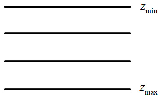
Figure 1.
Schematic diagram of layered media.
2.2. Boundary Conditions
There are usually no source terms at the upper and lower boundaries of the solution area, which means that the upper and lower boundaries are areas without sources, i.e., . Therefore, Equation (4) can be written at the upper and lower boundaries as
The general solution of this equation is
where represents the downgoing wave, while represents the upgoing wave. A and B are arbitrary constants. At the upper boundary , there is only the upgoing wave, and at the lower boundary , there is only the downgoing wave, i.e.,
Therefore, the boundary conditions can be obtained as
2.3. Boundary Value Problem Solution
Thus, the boundary value problem satisfied by the acoustic wave equation in the space-wavenumber domain of layered media is
The boundary value problem is solved using the Galerkin finite-element method.
By moving the source term on the right-hand side of the first equation in Equation (9) to the left-hand side, multiplying the equation by , and integrating, can obtain
The first term in the above equation, through integration by parts, can be expressed as
Substituting Equation (11) into Equation (10),
Dividing z into a series of elements, with a quadratic interpolation shape function N used within each element, Equation (12) can be rewritten as a finite-element equation:
where represents the number of elements in the vertical discretization. Due to the arbitrariness of , the finite-element equation can be simplified as
The element integrals of the finite-element equation include the following four forms, which can be determined by reference tables [28]:
The first integral form:
where l represents the element grid size vertically.
The second integral form:
The third integral form:
where
where represents the value corresponding to the element stiffness matrix; correspond to the critical wavenumbers at the three nodes within the element, respectively.
The fourth integral form:
where the boundary term is
where
Substituting Equations (15)–(20) into Equation (14) and performing global assembly, the following equation is obtained:
where ; is the source term matrix, which corresponds to the right-hand side of the equation. represents the wavefield of the layered medium in the spatial-wavenumber domain within the frequency domain, which is to be solved.
After obtaining the wavefield in the space-wavenumber domain, the space-domain wavefield can be calculated by performing an inverse Fourier transform in the horizontal directions.
2.4. NUFFT Theory
Due to the complex distribution of the acoustic wavefield in the wavenumber domain, a large number of wavenumbers must be selected to ensure the accuracy of the spectrum in the wavenumber domain, thereby obtaining an accurate space-domain wavefield distribution through the inverse Fourier transform. However, as the number of wavenumbers increases, the memory requirements of conventional fast Fourier transform (FFT) methods grow significantly, making it challenging to meet the demands of acoustic wavefield numerical simulations. Therefore, a Fourier transform method that is efficient and accurate, requires low memory, avoids truncation effects, and supports arbitrary non-uniform sampling becomes a critical step in solving the space-domain wavefield. To address this, this study employs the NUFFT method to achieve an accurate and efficient transformation from the wavenumber-domain wavefield to the space-domain wavefield.
Dutt first proposed NUFFT in 1993 [29]. Please refer to the literature for specific details about NUFFT [30,31,32,33,34]. Based on an approach similar to the gridding method, the NUFFT method first applies an appropriate scaling factor to correct the original data. Then, an oversampled intermediate sequence is computed using the FFT, and finally, the results are interpolated onto the target grid. The general NUFFT algorithm can be divided into three categories. The first type involves transforming uniformly distributed sampling values into sampling values at non-uniform positions through a Fourier transform, referred to as NER (Non-Equispaced Result). The second type performs a discrete Fourier transform on sampling data at non-uniform grid points to obtain uniformly distributed sampling values, known as NED (Non-Equispaced Data). The third type conducts a discrete Fourier transform on sampling data at non-uniform grid points to derive sampling values at non-uniform positions. These three categories are designed to handle different scenarios of data and sampling distributions in Fourier transform computations. In geophysical numerical simulations, non-uniform sampling is required in spatial and wavenumber domains. The third type of NUFFT algorithm is more suitable for addressing the challenges of solving partial differential equations in geophysical applications. For the NUFFT algorithm and program for computation, refer to the literature [31,32].
The 2D discrete Fourier transform is expressed by the following equation:
where represents the wavenumber-domain function, and denotes the spatial-domain function. represents uniform or non-uniform sampling points in the spatial domain, while corresponds to uniform or non-uniform sampling points in the wavenumber domain. When a non-uniform grid is used in the spatial domain, direct computation via FFT is not feasible. Instead, interpolation to a uniform grid is required, followed by the application of FFT to achieve NUFFT computation.
To interpolate the non-uniform grid onto a uniform grid, a 2D Gaussian kernel function is used for convolution:
where determines the sampling spacing in the space domain. The interpolated spatial-domain function is given by
The Fourier transform of the Gaussian kernel function can be expressed as
The computation of the interpolated spatial-domain function in Equation (25) can be expanded as
where represents the spatial-domain function on the uniform grid after convolution smoothing. It is also necessary to perform a deconvolution operation to reverse the smoothing effect introduced by the interpolation process, as given by the following equation:
Then, the deconvolved function is subjected to a Fourier transform:
The above equation can be efficiently computed using the standard FFT,
where represent the spacing between the spatial grid points, are the wavenumber discretization indices, and are the spatial-domain indices.
Through FFT, the transformation from the spatial uniform grid to the wavenumber uniform grid is realized. The next step also requires interpolation to the non-uniform wavenumber grid. First, a convolution operation is performed to map the data onto the non-uniform wavenumber-domain grid:
Then, through the deconvolution operation, the Fourier transform result on the non-uniform wavenumber grid is obtained:
The implementation process can be summarized as follows:
- Gaussian interpolation to uniform sampling points: Interpolate the non-uniform grid onto the uniform grid using Gaussian interpolation, obtaining .
- Deconvolution: Perform deconvolution on the values at each uniform grid point to obtain .
- FFT calculation: Perform standard FFT on the uniform grid points for , obtaining .
- Gaussian interpolation to non-uniform sampling points: Perform Gaussian interpolation to map the uniform grid points onto the non-uniform grid, obtaining .
- Deconvolution: Perform deconvolution to obtain the final transformation result .
In this study, the use of the NUFFT method is not limited to handling non-uniform sampling; more importantly, it addresses the issue in traditional fast Fourier transform (FFT) where once the spatial-domain sampling is determined, the sampling in the wavenumber domain is also fixed. In conventional FFT methods, the sampling interval and the maximum wavenumber in the wavenumber domain are directly determined by the spatial sampling interval and cannot be independently adjusted. In contrast, the NUFFT method overcomes this limitation, allowing for flexible adjustment of the sampling range in the wavenumber domain according to the specific needs, thus achieving higher accuracy with fewer sampling points. This characteristic provides a significant computational advantage of NUFFT in geophysical numerical simulations, particularly in the solution of partial differential equations for seismic wavefield modeling, enabling high precision while reducing computational costs.
2.5. Wavenumber Selection
The distribution of the acoustic wavefield in the wavenumber domain is highly complex, requiring the selection of a large number of wavenumbers to ensure the accuracy of the wavenumber spectrum, thereby enabling the accurate spatial-domain wavefield to be obtained through inverse Fourier transform. Therefore, an efficient and accurate Fourier transform method capable of arbitrary non-uniform sampling becomes a critical step in solving the spatial-domain wavefield. Additionally, Green’s function of a point source in the full-space acoustic wavefield provides insights into the wavefield’s distribution in the horizontal wavenumber domain, offering a basis for wavenumber selection.
Under full-space conditions, the analytical solution of the point source acoustic wavefield in the space-wavenumber domain is expressed as
where ; is the critical wavenumber, representing the singularity in the analytical solution of the point source in the whole space-wavenumber domain.
To understand the spectral distribution of the acoustic wavefield of a point source in the horizontal wavenumber domain under full-space conditions, a spatial-wavenumber-domain point source model is designed with the following parameters—kx: ~, ky: ~, and z: 0 km~2 km. The point source coordinates are (0 m, 0 m, 1 km). The acoustic wave velocity of the full-space medium is 1500 m/s, and the dominant frequency of the point source is 30 Hz. Frequencies of 5 Hz, 15 Hz, and 30 Hz are selected for the analysis.
The wavefield spectrum distribution of the point source is analyzed on the z = 0 m plane, as shown in Figure 2.
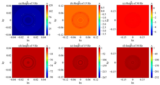
Figure 2.
The analytical solution of the wavenumber domain for a point source in full space on the z = 0 m plane. (a–c) represent the real parts of the wavefield spectra at frequencies of 5 Hz, 15 Hz, and 30 Hz, respectively, while (d–f) represent the imaginary parts of the wavefield spectra at frequencies of 5 Hz, 15 Hz, and 30 Hz, respectively.
Based on Huygens’ principle, the scattered field can be viewed as the superposition of secondary point sources at each scattering point [8,35]. That is, each point on the wavefront can be considered as a secondary point source, and the superposition of the waves emitted by these secondary point sources forms the subsequent wavefronts. Therefore, in the scattering field, each scattering point can be regarded as a secondary point source, which radiates energy in space, and these secondary waves combine to form the total scattered field. As a result, in scattering problems, each scattering point behaves like a point source, and the field it generates can be described using Green’s function. The entire scattering field is the superposition of all these Green’s functions in space. Thus, the distribution of the wavenumber domain’s Green’s function can provide guidance for selecting the appropriate wavenumber.
According to Green’s function of the point source acoustic wavefield, it decays rapidly beyond the critical wavenumber kc, and is equal to zero thereafter 2kc. Therefore, in the calculation of the layered media wavefield, the range of wavenumber selection is . The formula for calculating the critical wavenumber in multi-layer media is
The maximum critical wavenumber corresponding to the minimum velocity is used as the wavenumber selection range for the entire computational model.
2.6. Algorithm Flowchart
The flow of the algorithm is shown in Figure 3.
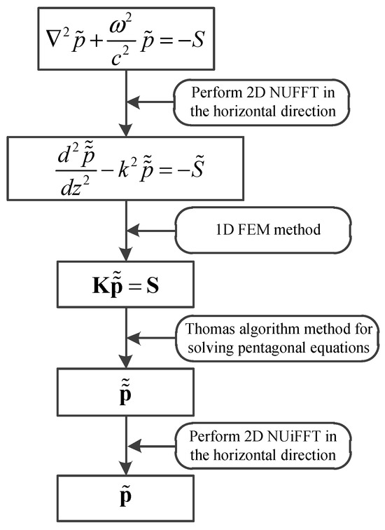
Figure 3.
Algorithm flowchart.
3. Results
Based on the solution theory of point source acoustic waves in layered media, a numerical simulation program was developed to verify the correctness of the algorithm by comparing it with the analytical solution of a whole space point source, and design half-space and three-layer medium models to analyze the acoustic wavefield response of point source layered media. The test model is an Intel i7 11800H, Core 2.3 GHz, 64 GB of memory.
To measure the accuracy of the algorithm, the relative root mean square error (Rrms) [36] is introduced, and the calculation formula is as follows:
where Nx and Ny represent the number of grid points in the x and y directions, respectively; is the numerical solution, and is the reference solution. The relative error is weighted differently for large and small numerical values. When calculating the error, the influence of the relative error on the larger numerical values is considered, with special attention given to the smaller numerical values that contribute to the total error.
3.1. Correctness Verification
A full-space point source model is designed and compared with analytical solutions to verify the correctness of the point source acoustic layered medium-solving algorithm. Calculate the model’s scope, x: −250 m~250 m, y: −250 m~250 m, and z: 0 m~100 m. The point source is located at the model’s center, with coordinates of (0 m, 0 m, 50 m). Choose the Rayleigh wave as the excitation source, with a main frequency of 15 Hz and a calculated frequency of 30 Hz. The medium velocity of the full-space model is 3000 m/s. Given that the spectral distribution of point sources in the wavenumber domain is already 0 in the region twice the critical wavenumber from zero, the range of wavenumbers kx and ky is −2kc~2kc, which is −0.216~0.216, and uniform sampling is used. The number of nodes Nx, Ny, and Nz in the three directions of the spatial domain is 401 × 401 × 601, respectively, and the number of sampling nodes Nkx and Nky in the wavenumber domain is 501 × 501.
For the convenience of analyzing the calculation results, the wavefield in the z = 0 m plane is selected and compared with the analytical solution, as shown in Figure 4. The numerical and analytical solutions have almost identical waveforms, with relative root mean square errors of less than 1% in real and imaginary parts, satisfying numerical accuracy and verifying the correctness of the algorithm.
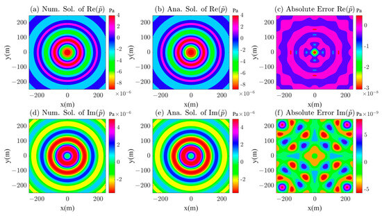
Figure 4.
The numerical solution, analytical solution, and absolute error of the point source in the full space of the z = 0 m plane. (a–c) are the numerical solution, analytical solution, and absolute error of the real part of the point source acoustic wavefield, respectively; (d–f) are the numerical solution, analytical solution, and absolute error of the imaginary part of the point source acoustic wavefield, respectively.
3.2. Half-Space Model
Design a half-space model as shown in Figure 5, and calculate the model range, x: −500 m~500 m, y: −500 m~500 m, and z: 0 m~500 m. The first layer of the medium is an air layer with a velocity of 340 m/s and a thickness of 250 m. The second layer of the medium has a velocity of 3000 m/s and a thickness of 250 m. The point source coordinates are (0 m, 0 m, 100 m), and the main frequency of the Rayleigh wave is 20 Hz. The calculated frequencies are 5 Hz, 10 Hz, and 20 Hz. The number of nodes Nx, Ny, and Nz in the three directions of the spatial domain is 501 × 501 × 501, respectively. The horizontal grid size is 2 m, and the vertical grid size is 1 m, which meets the requirements for use in the air layer. The range of wavenumbers kx and ky is −2kc~2kc. kc is based on the critical wavenumber corresponding to the minimum velocity, and uniform sampling is used. The number of sampling nodes Nkx and Nky is 501 × 501.
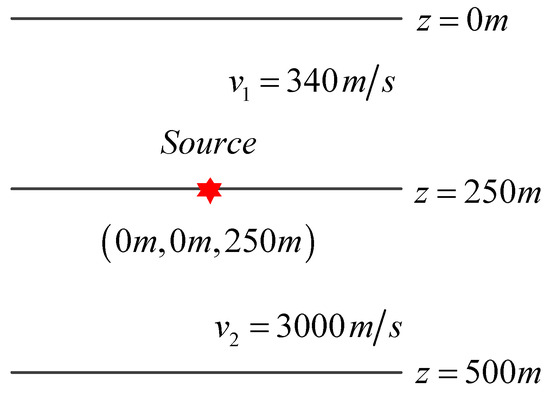
Figure 5.
Half-space model diagram. The red star represents a point source.
The distribution of real and imaginary wavefield profiles at different frequencies (5 Hz, 10 Hz, 20 Hz) 50 m away from the point source is shown in Figure 6. The frequency, propagation path, and medium properties of the waves jointly influence the wavefield distribution characteristics. Through this graph, the propagation laws and attenuation characteristics of waves with different frequencies can be intuitively observed. As the frequency increases, the wavelength of the wavefield significantly shortens, the distribution of peaks and valleys becomes more dense, and the local changes in fluctuations become more significant. Due to the use of the half-space assumption in the model, the wavefield distribution exhibits symmetry. From the figure, it can be observed that the main energy of the wavefield is concentrated near the source point and gradually decays with increasing propagation distance. At different frequencies, there are significant differences in the spatial distribution of the wavefield: low-frequency waves have a wide propagation range and larger amplitude, while high-frequency waves are limited to a smaller range and rapidly attenuate in amplitude. Due to the existence of the air layer, it is necessary to perform dense partitioning in the air layer, which requires high computational resources. Therefore, algorithms with low memory consumption and high efficiency are significant in considering the numerical simulation of layered acoustic waves in the air layer.
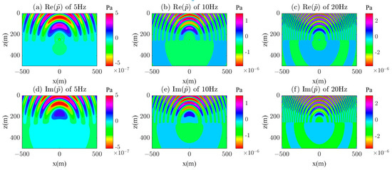
Figure 6.
Calculation results of the real and imaginary parts of the wavefield in the half-space of the y = 50 m section; (a) 5 Hz (real part), (b) 10 Hz (real part), (c) 20 Hz (real part), (d) 5 Hz (imaginary part), (e) 10 Hz (imaginary part), (f) 20 Hz (imaginary part).
Figure 7 shows the 3D distribution of the real and imaginary parts of the half-space wavefield, visualized at three frequencies of 5 Hz, 10 Hz, and 20 Hz, where (a), (c), and (e) represent the distribution of the real part of the wavefield, and (b), (d), and (f) represent the distribution of the imaginary part of the wavefield. The 3D distribution characteristics of the wavefield at different frequencies can be seen in the figure. As the frequency increases, the wavelength of the acoustic wave becomes smaller, especially in the air layer. This figure indicates that the algorithm proposed in this paper is suitable for the numerical simulation of acoustic wavefields in layered media containing air layers, and has high accuracy.
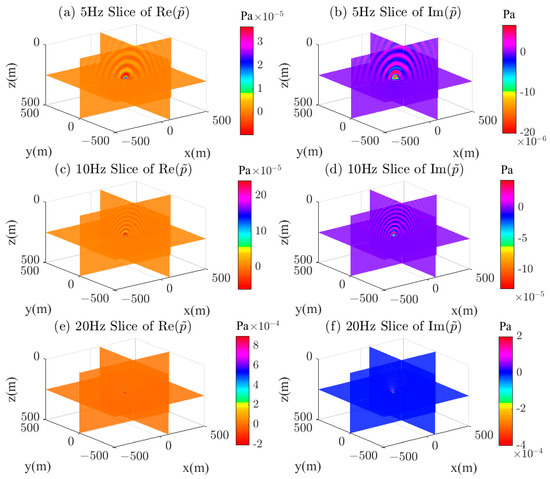
Figure 7.
A 3D display of the real and imaginary parts of the half-space wavefield; (a) 5 Hz (real part), (b) 5 Hz (imaginary part), (c) 10 Hz (real part), (d) 10 Hz (imaginary part), (e) 20 Hz (real part), (f) 20 Hz (imaginary part).
3.3. Three-Layer Medium Model
To analyze the response characteristics of the acoustic wavefield in the frequency domain under a three-layer medium, a three-layer medium model is designed as shown in Figure 8. Calculate the model’s scope, x: −500 m~500 m, y: −500 m~500 m, and z: 0 m~500 m. The first layer of the medium has a velocity of 1000 m/s and a thickness of 100 m. The second layer has a medium velocity of 2000 m/s and a thickness of 200 m. The third layer of the medium has a velocity of 3000 m/s and a thickness of 200 m. The point source coordinates are 200 m, and the main frequency of the Rayleigh wave is 20 Hz. The calculated frequencies are 5 Hz, 15 Hz, and 30 Hz. The number of nodes Nx, Ny, and Nz in the three directions of the spatial domain is 201 × 201 × 201, respectively. The horizontal grid size is 5 m, and the vertical grid size is 2.5 m, which meets the sampling requirements. The range of wavenumbers kx and ky is −2kc~2kc. kc is based on the critical wavenumber corresponding to the minimum velocity, and uniform sampling is used. The number of sampling nodes Nkx and Nky is 501 × 501.
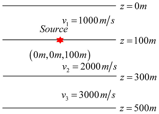
Figure 8.
Three-layer medium model diagram. The red star represents a point source.
The distribution of real and imaginary wavefield profiles at different frequencies (5 Hz, 15 Hz, 30 Hz) 50 m away from the point source is shown in Figure 9. From the figure, it can be seen that the frequency-domain wavefield exhibits obvious layered characteristics, and at different frequencies, as the frequency increases, the wavelength of the wavefield becomes shorter, and the resolution becomes higher. At different depths, the higher the velocity, the longer the wavelength, and the lower the resolution, which is consistent with the pattern found in actual seismic exploration. This again demonstrates that the algorithm proposed in this paper is suitable for the high-precision calculation of point source layered acoustic wavefields, providing an essential basis for studying seismic waves’ propagation characteristics and energy dissipation mechanism. In addition, these characteristics can give guidance for full-waveform inversion imaging.
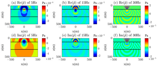
Figure 9.
Calculation results of the real and imaginary parts of the wavefield in the half-space of the y = 50 m profile; (a) 5 Hz (real part), (b) 15 Hz (real part), (c) 30 Hz (real part), (d) 5 Hz (imaginary part), (e) 15 Hz (imaginary part), (f) 30 Hz (imaginary part).
Figure 10 shows the 3D distribution of the real and imaginary parts of the wavefield under a three-layer medium model. The wavefield is visualized in three dimensions at frequencies of 5 Hz, 15 Hz, and 30 Hz, where (a), (c), and (e) represent the distribution of the real part of the wavefield, and (b), (d), and (f) represent the distribution of the imaginary part of the wavefield. The 3D layered wavefield shows a cylindrical symmetric distribution concerning the point source. The 3D wavefield diagram shows that the wavefield exhibits diffusion characteristics in the calculation area at low frequencies, with low resolution. At high frequencies, it exhibits significant volatility and high resolution. And as the depth increases, the wave velocity increases, the wavelength becomes longer, and the resolution decreases.
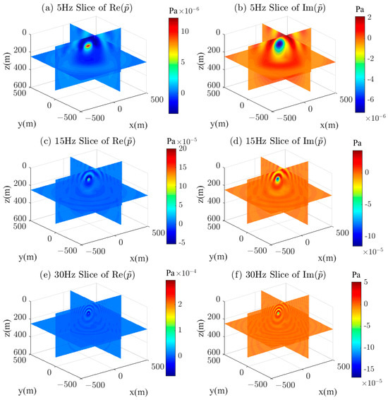
Figure 10.
A 3D display of the real and imaginary parts of the half-space wavefield; (a) 5 Hz (real part), (b) 5 Hz (imaginary part), (c) 15 Hz (real part), (d) 15 Hz (imaginary part), (e) 30 Hz (real part), (f) 30 Hz (imaginary part).
3.4. Sensitivity Analysis
It is crucial to analyze the impact of model parameters on algorithm accuracy. This section analyzes the influence of the grid node number, medium velocity, and source frequency on algorithm accuracy under the full-space model.
3.4.1. Grid Nodes
Select a full-space model with a point source of a 20 Hz Rayleigh wavelet, calculated frequency of 20 Hz, and medium velocity of 3000 m/s. The range of wavenumbers is −2kc~2kc. The accuracy statistics of the wavefield by changing the mesh division separately are shown in Table 1. It can be seen that the denser the spatial-domain partitioning, the more wavenumbers are selected, and the higher the accuracy of the algorithm.

Table 1.
Algorithm accuracy with different grid nodes.
3.4.2. Medium Velocity
Select a full-space model with a point source of a 20 Hz Rayleigh wavelet, calculated frequency of 20 Hz, and medium velocities of 1000 m/s, 2000 m/s, 3000 m/s, 4000 m/s, and 5000 m/s, respectively. The range of wavenumbers is −2kc~2kc. The number of nodes in the spatial domain is 501 × 501 × 501, and the number of nodes in the wavenumber domain is 501 × 501. The accuracy statistics of the wavefield under different medium velocities are shown in Table 2. It can be seen that the higher the medium velocity, the higher the algorithm accuracy. The reason is that the lower the wave velocity, the smoother the spectrum, and the smaller the critical wavenumber. When the number of wavenumbers selected is the same, the algorithm accuracy will improve with the increase in velocity. However, the algorithm accuracy still meets the requirements at low speeds.
Table 2.
Algorithm accuracy under different medium velocities.
3.4.3. Source Frequency
Select a full-space model with a point source of a 20 Hz Rayleigh wave and medium velocities of 3000 m/s. The range of wavenumbers is −2kc~2kc. The number of nodes in the spatial domain is 501 × 501 × 501, and the number of nodes in the wavenumber domain is 501 × 501. The accuracy statistics of the wavefield at different frequencies of 10 Hz, 20 Hz, 30 Hz, 40 Hz, and 50 Hz are shown in Table 3. It can be seen that the higher the frequency of the point source, the lower the accuracy of the algorithm. The reason for this is that as the frequency increases, the frequency spectrum oscillates more and more, and the critical wavenumber increases. When the number of wavenumbers selected is the same, the accuracy of the algorithm decreases with the increase in frequency. However, the accuracy of the algorithm still meets the requirements at high frequencies.
Table 3.
Algorithm accuracy under different source frequencies.
3.5. Efficiency and Memory Usage
To analyze the algorithm’s performance, the algorithm’s calculation time and memory usage were calculated for different grid divisions and wavenumbers at a single frequency, as shown in Table 4. The table shows that the more grid nodes there are, the more memory and time are required for computation. When the horizontal grid Nx, Ny and the number of wavenumbers Nkx, Nky remain unchanged, and the vertical grid Nz doubles, the computation time doubles, and the memory expands approximately twice. When the vertical grid Nz remains constant and the number of horizontal grids and wavenumbers is increased by four times, the calculation time increases by four times. When the vertical grid and the horizontal spatial grid remain unchanged, and the number of wavenumbers is increased by four times, the calculation time increases by about 2.5 times. On the contrary, when the vertical grid and the number of wavenumbers remain constant, and the horizontal spatial domain is expanded by four times, the calculation time increases by about 2.3 times. It can be seen that the increase in the number of wavenumbers has a more significant impact on the calculation efficiency. When the vertical grid is doubled and the number of horizontal grids and wavenumbers is quadrupled, the calculation time increases by 8 times. In the spatial domain of 501 × 501 × 501 and the wavenumber domain of 501 × 501, calculating a frequency takes about 6 min. It only occupies 4 Gb of memory, which can fully leverage its advantages in large-scale seismic numerical simulation and waveform inversion.
Table 4.
Statistics of Algorithm Efficiency and Memory Usage under Different Grids and Wavenumbers with Single Frequency.
To highlight the advantages of the algorithm presented in this paper, a conventional FEM algorithm was chosen. The algorithm efficiency and memory usage at different nodes under regular grid discretization are shown in Table 5. From the table, it can be seen that the FEM algorithm, with a grid size of 61 × 61 × 31, reaches a memory usage of 49 GB and takes 296.6 s, and for grid sizes larger than this, the calculation is not feasible on the test computer. In contrast, the algorithm proposed in this paper, with a grid size of 101 × 101 × 101 and a wavenumber domain of 101 × 101, takes only 3.8 s and uses just 0.35 GB of memory. This clearly demonstrates that the proposed algorithm significantly outperforms the traditional finite-element algorithm.
Table 5.
Efficiency and memory usage statistics of the FEM algorithm at different grid sizes for a single frequency.
4. Conclusions
This paper proposes a numerical solution method for the 3D frequency-domain point source acoustic equation in layered media, which addresses the problem of difficulty in balancing efficiency and accuracy in solving the acoustic wavefield in layered media. NUFFT is used to achieve arbitrary sampling. A horizontal 2D Fourier transform on the 3D acoustic wave equation transforms it into a one-dimensional space-wavenumber-domain ordinary differential equation, thereby reducing a large 3D problem to a one-dimensional problem and greatly reducing the memory requirements. The one-dimensional finite-element method is used to obtain the pentagonal equation, and the pursuit method is used to solve the spatial-wavenumber-domain layered wavefield distribution efficiently. Finally, the inverse 2D Fourier transform obtains the spatial-domain wavefield distribution. Through algorithm correctness verification and a case analysis, it is shown that the point source layered medium algorithm proposed in this paper can accurately calculate the wavefield distribution in the air layer when considering the air layer. Meanwhile, the algorithm demonstrates high efficiency and computational stability in ultra-large-scale models. In testing the three-layer medium model, the adaptability and accuracy of the algorithm proposed in this paper in calculating the distribution of acoustic waves in layered media were further verified. The algorithm efficiency analysis found that this method has extremely low memory usage and high computational efficiency and can quickly solve large-scale models even on ordinary computers. The method proposed in this article provides an efficient, flexible, and accurate solution for simulating 3D acoustic wavefields in layered media.
The acoustic layered medium calculation method proposed in this article provides a new approach for solving partial differential equations and proposes an efficient and feasible solution for background field calculation in scattering seismic numerical simulations, opening up new directions for research on such problems. In addition, this method has shown significant potential for application in the full-waveform inversion of acoustic waves, laying a solid foundation for improving the accuracy and efficiency of full-waveform inversion. Therefore, this work has important theoretical significance and practical value in studying partial differential equation solving and seismic wavefield simulation.
Author Contributions
Conceptualization, S.D. and Y.Z.; methodology, Y.Z.; validation, Y.Z.; formal analysis, Y.Z.; investigation, Y.Z.; writing—original draft preparation, Y.Z.; writing—review and editing, Y.Z.; visualization, Y.Z.; supervision, S.D.; project administration, S.D. and Y.Z.; funding acquisition, S.D. All authors have read and agreed to the published version of the manuscript.
Funding
This research was funded by the National Natural Science Foundation of China (No. 41574127).
Data Availability Statement
Data are contained within the article.
Conflicts of Interest
The authors declare no conflicts of interest.
References
- Aki, K.; Richards, P.G. Quantitative Seismology, 2nd ed.; University Science Books: Santa Cruz, CA, USA, 2002. [Google Scholar]
- Ben-Menahem, A.; Jit Singh, S. Multipolar Elastic Fields in a Layered Half Space. Bull. Seismol. Soc. Am. 1968, 58, 1519–1572. [Google Scholar] [CrossRef]
- Chen, X.; Zhang, H. An Efficient Method for Computing Green’s Functions for a Layered Half-Space at Large Epicentral Distances. Bull. Seismol. Soc. Am. 2001, 91, 858–869. [Google Scholar] [CrossRef]
- Liu, S.; Zhou, Z.; Dai, S.; Iqbal, I.; Yang, Y. Fast Computation of Green Function for Layered Seismic Field via Discrete Complex Image Method and Double Exponential Rules. Symmetry 2021, 13, 1969. [Google Scholar] [CrossRef]
- Ouyang, F.; Zhao, J.; Dai, S.; Wang, S. Seismic Wave Modeling in Vertically Varying Viscoelastic Media with General Anisotropy. Geophysics 2021, 86, T211–T227. [Google Scholar] [CrossRef]
- Liu, W.; Wang, H.; Xi, Z.; Wang, L.; Chen, C.; Guo, T.; Yan, M.; Wang, T. Multitask Learning-Driven Physics-Guided Deep Learning Magnetotelluric Inversion. IEEE Trans. Geosci. Remote Sens. 2024, 62, 5926416. [Google Scholar] [CrossRef]
- Liu, W.; Wang, H.; Xi, Z.; Zhang, R.; Huang, X. Physics-Driven Deep Learning Inversion with Application to Magnetotelluric. Remote Sens. 2022, 14, 3218. [Google Scholar] [CrossRef]
- Buchwald, V.T. Elastic Waves in Anisotropic Media. Proc. R. Soc. Lond. 1959, 253, 563–580. [Google Scholar]
- Bufler, H. Theory of Elasticity of a Multilayered Medium. J. Elast. 1971, 1, 125–143. Available online: https://link.springer.com/article/10.1007/BF00046464 (accessed on 2 January 2025). [CrossRef]
- Bahar, L.Y. Transfer Matrix Approach to Layered Systems. J. Eng. Mech. Div. 1972, 98, 1159–1172. [Google Scholar] [CrossRef]
- Kattis, S.E.; Beskos, D.E.; Cheng, A.H.D. 2D Dynamic Response of Unlined and Lined Tunnels in Poroelastic Soil to Harmonic Body Waves. Earthq. Eng. Struct. Dynamlcs 2003, 32, 97–100. [Google Scholar] [CrossRef]
- Ciz, R.; Gurevich, B. Amplitude of Biot’s Slow Wave Scattered by a Spherical Inclusion in a Fluid-Saturated Poroelastic Medium. Geophys. J. Int. 2005, 160, 991–1005. [Google Scholar] [CrossRef]
- Weihua, L.; Chenggang, Z. Scattering of Plane SV Waves by Cylindrical Canyons in Saturated Porous Medium. Soil Dyn. Earthq. Eng. 2005, 25, 981–995. [Google Scholar] [CrossRef]
- Hasheminejad, S.M.; Avazmohammadi, R. Harmonic Wave Diffraction by Two Circular Cavities in a Poroelastic Formation. Soil Dyn. Earthq. Eng. 2007, 27, 29–41. [Google Scholar] [CrossRef]
- Hasheminejad, S.M.; Avazmohammadi, R. Dynamic Stress Concentrations in Lined Twin Tunnels within Fluid-Saturated Soil. J. Eng. Mech. 2008, 137, 542–554. [Google Scholar] [CrossRef]
- Jiang, L.-F.; Zhou, X.-L.; Wang, J.-H. Scattering of a Plane Wave by a Lined Cylindrical Cavity in a Poroelastic Half-Plane. Comput. Geotech. 2009, 36, 773–786. [Google Scholar] [CrossRef]
- Liu, X.; Greenhalgh, S.; Zhou, B. Scattering of Plane Transverse Waves by Spherical Inclusions in a Poroelastic Medium. Geophys. J. Int. 2009, 176, 938–950. [Google Scholar] [CrossRef]
- Trifunac, M.D. Scattering of Plane Sh Waves by a Semi-cylindrical Canyon. Earthq. Eng. Struct. Dyn. 1972, 1, 267–281. [Google Scholar] [CrossRef]
- Zhang, N.; Zhang, Y.; Gao, Y.; Pak, R.Y.S.; Wu, Y.; Zhang, F. An Exact Solution for SH-Wave Scattering by a Radially Multilayered Inhomogeneous Semicylindrical Canyon. Geophys. J. Int. 2019, 217, 1232–1260. [Google Scholar] [CrossRef]
- Liu, Q.; Zhao, M.; Liu, Z. Wave Function Expansion Method for the Scattering of SH Waves by Two Symmetrical Circular Cavities in Two Bonded Exponentially Graded Half Spaces. Eng. Anal. Bound. Elem. 2019, 106, 389–396. [Google Scholar] [CrossRef]
- Alterman, Z.; Karal, F.C., Jr. Propagation of Elastic Waves in Layered Media by Finite Difference Methods. Bull. Seismol. Soc. Am. 1968, 58, 367–398. [Google Scholar]
- JafarGandomi, A.; Takenaka, H. Efficient FDTD Algorithm for Plane-Wave Simulation for Vertically Heterogeneous Attenuative Media. Geophysics 2007, 72, A47–Z71. [Google Scholar] [CrossRef]
- JafarGandomi, A.; Takenaka, H. FDTD3C—A FORTRAN Program to Model Multi-Component Seismic Waves for Vertically Heterogeneous Attenuative Media. Comput. Geosci. 2013, 51, 314–323. [Google Scholar] [CrossRef]
- Sheikhhassani, R.; Dravinski, M. Dynamic Stress Concentration for Multiple Multilayered Inclusions Embedded in an Elastic Half-Space Subjected to SH-Waves. Wave Motion 2016, 62, 20–40. [Google Scholar] [CrossRef]
- Sotelo, E.; Favino, M.; Jr, R.L.G. Application of the Generalized Finite-Element Method to the Acoustic Wave Simulation in Exploration Seismology. Geophysics 2021, 86, T61–T74. [Google Scholar] [CrossRef]
- Lei, W.; Liu, Y.; Li, G.; Zhu, S.; Chen, G.; Li, C. 2D Frequency-Domain Finite-Difference Acoustic Wave Modeling Using Optimized Perfectly Matched Layers. Geophysics 2023, 88, F1–F13. [Google Scholar] [CrossRef]
- Altybay, A.; Tokmagambetov, N. Numerical Simulation and Parallel Computing of Acoustic Wave Equation in Isotropic-Heterogeneous Media. CMES Comput. Model. Eng. Sci. 2024, 141, 1867–1881. [Google Scholar] [CrossRef]
- Xu, S. The Finite Element Method in Geophysics; Science Press: Beijing, China, 1994. [Google Scholar]
- Dutt, A.; Rokhlin, V. Fast Fourier Transforms for Nonequispaced Data. Siam J. Sci. Comput. 1993, 14, 1368–1393. [Google Scholar] [CrossRef]
- Fessler, J.A.; Sutton, B.P. Nonuniform Fast Fourier Transforms Using Min-Max Interpolation. IEEE Trans. Signal Process. 2003, 51, 560–574. [Google Scholar] [CrossRef]
- Greengard, L.; Lee, J.-Y. Accelerating the Nonuniform Fast Fourier Transform. SIAM Rev. 2004, 46, 443–454. [Google Scholar] [CrossRef]
- Lee, J.-Y.; Greengard, L. The Type 3 Nonuniform FFT and Its Applications. J. Comput. Phys. 2005, 206, 1–5. [Google Scholar] [CrossRef]
- Keiner, J.; Kunis, S.; Potts, D. Fast Summation of Radial Functions on the Sphere. Computing 2006, 78, 1–15. [Google Scholar] [CrossRef]
- Keiner, J.; Kunis, S.; Potts, D. Using NFFT 3—A Software Library for Various Nonequispaced Fast Fourier Transforms. ACM Trans. Math. Softw. 2009, 36, 1–30. [Google Scholar] [CrossRef]
- Dissanayake, D. Acoustic Waves; BoD—Books on Demand; Intechopen: London, UK, 2010; ISBN 978-953-307-111-4. [Google Scholar]
- Wu, L. Efficient Modelling of Gravity Effects Due to Topographic Masses Using the Gauss-FFT Method. Geophys. J. Int. 2016, 205, 160–178. [Google Scholar] [CrossRef]
Disclaimer/Publisher’s Note: The statements, opinions and data contained in all publications are solely those of the individual author(s) and contributor(s) and not of MDPI and/or the editor(s). MDPI and/or the editor(s) disclaim responsibility for any injury to people or property resulting from any ideas, methods, instructions or products referred to in the content. |
© 2025 by the authors. Licensee MDPI, Basel, Switzerland. This article is an open access article distributed under the terms and conditions of the Creative Commons Attribution (CC BY) license (https://creativecommons.org/licenses/by/4.0/).