Comparison and Competition of Traditional and Visualized Secondary Mathematics Education Approaches: Random Sampling and Mathematical Models Under Neural Network Approach

Abstract

Graphic design and image processes have a vital role in information technologies and safe, memorable learning activities, which can meet the need for modern and visual aids in the field of education. In this article, the concepts of comparison and competition have been presented using grades or numbers obtained for two different intelligence quotient (IQ) classes of students. The two classes are categorized as learners having textual (un-visualized) and visualized aids. We use the results and outcomes of the random sampling data of the two classes in the parameters of four different, competitive, two-compartmental mathematical models. One of the compartments is for students who only learn through textual learning, and the other one is for students who have access to visualized text resources. Four of the mathematical models were solved numerically, and their grades were obtained by different iterations using the data of the mean of different random sampling tests taken for thirty months; each sampling involved thirty students. The said data are also drawn by using a neural network approach, showing the fitting curves for all the data, the training data, the validation data, and the testing data with histogram, aggression, mean square error, and absolute error. The obtained dynamics are also compared with neural network dynamics. The results of the scenario pointed out that the best results (determined through high grades) were obtained among the students of visual aid learners, as compared to textual and conventional learners. The visualized resources, constructed within the mathematics syllabus domain, may help to upgrade multidimensional mathematical education and the learning activities of intermediate-level students. For this, the findings of the present study are helpful for education policymakers: there is a directive to focus on visual-based learning, utilizing data from various surveys, profile checks, and questionnaires. Furthermore, the techniques presented in this article will be beneficial for those seeking to build a better understanding of the various methods and ideas related to mathematics education.

1. Introduction

The traditional and conventional education industry supports two-way student–teacher information communication, and there is no third party involvement. Through this process, only the text-based curriculum focuses on the learning, speaking, and listening skills of students. The related materials and extracurricular activities required for the practical application of the learning may not be available to students engaged in conventional learning. To avoid such deficiencies, educationalists have made different policies to link the objectives of the learning process with real life and practical uses. They have plans for encouraging students to accept their ideologies, for ensuring that they will be good citizens for their countries, for ensuring they will be beneficial and constructive in different services and departments in their countries, and for ensuring they will be ready to make new materials for import and export purposes. These are objectives of policymakers, compelling them to transition from conventional systems to modern visualized education systems [1].

In 2021, China improved the informative learning rates of both students and their instructors by developing the constructive information education model and accelerating the development of a literacy network among students [1]. They developed digital means of education by integrating digital transformations, ensuring that intelligent requirements were upgraded, deepening neural networking, and engaging in the continuous innovation of their applications [2]. After one year, in 2022, they also focused on the digitalization of all information related to literacy and the education industry [2]. The Education Ministry highlighted the main points for modern techniques to build novel infrastructures and enhance different paths for the supply of digitalization resources, deepening the information transmitted through education with the use of information technologies [3]. Later on, it was mentioned that the different literacy and education problems that arise may be remedied using information technologies and with improved teaching strategies. The aforementioned techniques have many more advantages and are important in the modern era of education [3]. With the passage of time, and with the development of information technology in teaching and learning, we have discovered that it is necessary to enhance the king of education that is delivered [4]. Teaching and learning through information technologies involve the production of new methods of transferring knowledge; such methods are not possible through conventional teaching approaches. Therefore, policymakers chose to develop teaching and learning approaches through the use of information technologies, supporting the development and reform of education.

In incorporating advanced technologies into education, educationalists are mostly interested in methods of visualized teaching, which include text images, graphs, tables, and charts, as well as dynamic media like animations, projectors, multimedia, screens, and cameras. The aforesaid apparatuses are the best resources for supporting learning and understanding among students of different IQ levels [5]. Such resources are especially necessary for learning mathematics; this subject requires an understanding of the geometries of different shapes and sizes in relationship to other variables like time, height, length, width, income, and price, both directly and indirectly. Furthermore, the coding and programming for each mathematical principle and image are constructed in different software languages; these take memorable forms, supporting a better understanding of mathematics when learning. This helps students: if they know that, behind each output in the form of objects seen on their computer, camera, LCD screen, or mobile screen, there is a 0 and 1, then they can understand the form which the mathematical model or equation (formula) uses to produce an output [5,6,7].

The authors of [8] pointed out that the visualized processes of learning improves student understanding of different arithmetic operations, providing the best usage of image-producing software. The authors of [9] show the development of students’ skills in various topics of mathematics through the application of proper visual teaching methods. The GeoGbrae visualization software focuses on geometrical shapes, algebra, and statistical reasoning; having extra dynamics leads to new approaches to teaching mathematics [9]. The authors of [10] assign properties to GeoGbrae for mathematics teaching; there are visual aids that present the importance of visual education in mathematics through the dynamics of quadrilateral characteristics.

Mathematical processes, communicated through visualized teaching, are completely changed in comparison with conventional methods; this is achievable through the inclusion of the GeoGbrae application in the classroom [11]. In [12], such modern approaches are used to convert information from an abstract form to a material form: this can involve the shift from static to dynamic media and that from text to maps and charts, all achievable through the use of proper software and visualized aids. Some limitations in modern mathematics lessons can be seen in their theoretical approaches and their conversion of abstract ideas to real, visualized schemes.

Researchers have performed work on the feasibility of applying visual resources for students and teachers. In [13], image construction techniques for secondary mathematics texts using Generative Adversarial Networks (GANs), with optimized rules for the generator and the discriminator, were highlighted; here, the researchers used upsampled and downsampled criteria for well-seen images. The GAN fails to ensure convergence when the sampling environment is small. To counter such drawbacks, the method was modified to use Deep Convolutional Generative Adversarial Networks (DCGANs) [13,14]. The researchers provided some experimental results from different statistical experiments, showing an enhancement in the performance of learners using these approaches.

Many works in the literature have used Neural Networks (NN) in various fields of mathematics, engineering, and other applied sciences. A neural network is composed of convolution layers, which are the dot product of a window of data and kernels of convolutions, with neurons and weights in the form of a two-dimensional matrix that is responsible for color and contour image processing [15,16,17,18]. A Deep Convolutional Generative Adversarial Network (DCGAN) works on the principles and coding of neural networks. The structure and operation of the human brain serve as inspiration for neural networks (NNs), which are computational models based on mathematical equations and vector–matrix products, made up of interconnected layers of nodes (neurons) that process input data for training, validating, and testing, thereby discovering intricate patterns.

The models studied under the NN approach are particularly effective in tasks such as classification, regression, and pattern recognition. Deep Neural Networks (DNNs) like the Residual Network (ResNet) [19] and the Feature Cross-Layer Interaction Hybrid Method, based on Res2Net and Transformer (FCIHMRT) [20], are advanced technologies of neural networking with multiple hidden layers between the input and output, enabling them to capture hierarchical features and model highly nonlinear relationships. Due to their increased depth and capacity, DNNs have achieved remarkable success in various fields, including image processing, natural language understanding, and scientific computing. Therefore, a number of research articles have been published in the literature [21,22,23,24] on this subject.

Mathematical tools may also be used to determine the performances of and competition among students engaged in conventional and visualized learning methods through statistical experiments [25]. From those experiments, the values of different parameters used in the mathematical equation can be easily found. Different mathematical equations of slopes and regression analyses comprise different parameters, which are calculated by various sampling techniques or preexisting data. Among these tools, one of the significant and important tools is that of mathematical modeling, which represents different biological, physical, sociological, chemical, computational networking, and economical problems [26,27]. Stochastic mathematical models mostly use probability techniques. Over the years, researchers have employed a wide variety of analytical and numerical methodologies to study and develop the mathematical models that are tailored to complex systems. These approaches have enabled a deeper understanding of the models’ structural properties and facilitated their application to diverse real-world problems across multiple scenarios [28,29,30,31]. Furthermore, different competitions in the search for food, minerals, technologies, educations systems, and territories can be formulated using mathematical models [32,33,34,35,36,37].

1.1. Objectives of the Proposed Research

The main aim of this research is to address our research questions through proper analysis. Accordingly, the present study is designed to fulfill its objectives comprehensively. The primary objectives are outlined as follows:

• To investigate the competition between two groups of students via different learning environments through examinations.
• To represent student competitions by four different mathematical models.
• To parameterize mathematical models by continuous random sampling from two different groups of students.
• To solve these mathematical models using a series-type solution.
• To provide dynamics through a numerical simulation for the validation of the obtained scheme.
• To check the significance of random sampling, the data will be tested, trained, and validated through a neural network analysis in the form of histograms and regression mean square and absolute error calculations.
• To conclude the findings of each group’s performance.

The above research objectives will answer the following research questions:

• How can we investigate competition between two groups of students who are engaged in different learning environments?
• How can we represent student competition using mathematical models?
• How can we parameterize mathematical models through continuous random sampling?
• How can we solve the mathematical models through a series-type solution?
• How can we provide graphical dynamics and their validation for the obtained scheme?
• How can we check the significance of random sampling?
• How can we conclude the outcomes of each group’s performance?

1.2. Competition Models with Limitations

In this article, mathematical models—used to understand a competition in the form of grades or IQ level between two types of students (learners)—are applied using data from unbiased continuous random sampling. Such types of mathematical models may also be used to assess other forms of competition: student enrollment, food, arms, technology, etc. One mathematical model can be used for different real-world phenomena. Here, in this article, each mathematical models has two differential equations. The first equation is for the first group of students, who are engaged in traditional or conventional teaching methods; the second equation is for the second group of students, who are engaged in visualized teaching. It was also possible, here, to examine the same group of students both when they were engaged in traditional learning methods (pre-test) and when they were engaged in visualized learning methods (post-test). The novelty of this study can be seen in the comparisons that we conduct among the outcomes (performances) of two classes of students who are engaged in different learning environments; these comparisons were conducted via a random sampling experiment (which was conducted six times within a period of five months) and parametrization using the mathematical models (see Example 4, Section 2). The dynamics of the mathematical models are compared with neural network dynamics, which use the data from the random sampling. These data are given in the tables and figures within the manuscript.

Four equations [37] are given in this section. The first equation is the popular population-like growth equation:

$$\begin{array}{c}\hfill \begin{array}{cc}& {\displaystyle \frac{d{S}_T\left(t\right)}{dt}}=\alpha S_T\left(t\right),\hfill \\ & {\displaystyle \frac{d{S}_V\left(t\right)}{dt}}=\beta S_V\left(t\right),\hfill \\ & S_T\left(0\right)=S_{T_0},S_V\left(0\right)=S_{V_0}.\hfill \end{array}\end{array}$$

(1)

where $S_T\left(t\right)$ is the number or grades acquired among students engaged in textual (traditional) learning; $S_V\left(t\right)$ is number or grades acquired among students engaged in visualized learning; $S_{T_0}$ and $S_{V_0}$ are the initial numbers or grades acquired by both groups of students; $\alpha$ and $\beta$ are the growth rates for $S_T\left(t\right)$ and $S_V\left(t\right)$. The values of these will be taken as the pre-test data for $\alpha$ and the post-test data, following the use of the visualized resources.

The second equation is the linear competition model: [37]

$$\begin{array}{c}\hfill \begin{array}{cc}& {\displaystyle \frac{d{S}_T\left(t\right)}{dt}}=\alpha S_T\left(t\right)-\gamma S_V\left(t\right),\hfill \\ & {\displaystyle \frac{d{S}_V\left(t\right)}{dt}}=\beta S_V\left(t\right)-\delta S_T\left(t\right),\hfill \\ & S_T\left(0\right)=S_{T_0},S_V\left(0\right)=S_{V_0}.\hfill \end{array}\end{array}$$

(2)

where $\gamma$ is the decreasing rate for the first group of students, or their grading, with the inclusion of the other group of students (those engaged in visualized learning). $\delta$ represents the decreasing rate for the second group of students (those engaged in visualized learning), which decreases due to the inclusion of the group of students engaged in text-based learning.

The third equation is the nonlinear competitive model [37]:

$$\begin{array}{c}\hfill \begin{array}{cc}& {\displaystyle \frac{d{S}_T\left(t\right)}{dt}}=\alpha S_T\left(t\right)-\gamma S_T\left(t\right)S_V\left(t\right),\hfill \\ & {\displaystyle \frac{d{S}_V\left(t\right)}{dt}}=\beta S_V\left(t\right)-\delta S_V\left(t\right)S_T\left(t\right),\hfill \\ & S_T\left(0\right)=S_{T_0},S_V\left(0\right)=S_{V_0}.\hfill \end{array}\end{array}$$

(3)

where $\gamma$ and $\delta$ are the same decreasing rates due to the effect of one grade on another grade. The fourth equation is the logistic-type competitive model [37]:

$$\begin{array}{c}\hfill \begin{array}{cc}& {\displaystyle \frac{d{S}_T\left(t\right)}{dt}}=a{S}_T\left(t\right)-b{S}_T^2\left(t\right)-c{S}_T\left(t\right)S_V\left(t\right),\hfill \\ & {\displaystyle \frac{d{S}_V\left(t\right)}{dt}}=a_1{S}_V\left(t\right)-b_1{S}_V^2\left(t\right)-c_1{S}_T\left(t\right)S_V\left(t\right),\hfill \\ & S_T\left(0\right)=S_{T_0},S_V\left(0\right)=S_{V_0}.\hfill \end{array}\end{array}$$

(4)

Here, a and $a_1$ are the increasing rates in the form of recruitment; b and $b_1$ are the decreasing rates by the removal of the number or the grades; c and $c_1$ are the decreasing rates by the effect of one group on another. Equation (4) can be written as follows:

$$\begin{array}{c}\hfill \begin{array}{cc}& {\displaystyle \frac{d{S}_T\left(t\right)}{dt}}=S_T\left(t\right)\left(a-b{S}_T\left(t\right)-c{S}_V\left(t\right)\right),\hfill \\ & {\displaystyle \frac{d{S}_V\left(t\right)}{dt}}=S_V\left(t\right)\left(a_1-b_1{S}_V\left(t\right)-c_1{S}_T\left(t\right)\right),\hfill \\ & S_T\left(0\right)=S_{T_0},S_V\left(0\right)=S_{V_0}.\hfill \end{array}\end{array}$$

(5)

2. Preliminaries

Definition 1.

Mathematical model: The representation of real-world phenomena (sociological, physical, biological, or economical) in mathematical form is called a mathematical model, and the process of making it is called mathematical modeling. It is composed of variables (unknown quantity), parameters, and constant terms. Mathematical models may take deterministic, stochastic, or difference equation forms. $F=ma$ is a mathematical model for Newton’s second law of motion; $F_{ac}=-F_{re}$ is the third law of motion. If $F_{external}=0$, then the body will be at rest. In uniform motion, which is the first law of motion. Some other examples of the mathematical models are presented here.

Example 1.

$$y\left(t\right)=mt+c$$

represents slope (m) intercept(c) form of any quantity, which may increase or decrease. Furthermore, the following

$${\displaystyle \frac{dP\left(t\right)}{dt}}=kP\left(t\right),P\left(0\right)=P_0,k>0$$

$${\displaystyle \frac{dN\left(t\right)}{dt}}=kN\left(t\right),N\left(0\right)=N_0,k<0$$

$${\displaystyle \frac{dI\left(t\right)}{dt}}=kI\left(t\right),I\left(0\right)=I_0,k>0$$

$${\displaystyle \frac{dS\left(t\right)}{dt}}=kS\left(t\right),S\left(0\right)=S_0,k>0$$

are the same equation but changed to represent different phenomena [37]. The first one refers to population growth, the second one refers to radioactive decay, the third one refers to disease growth or expansion, and the fourth one refers to interest amount, depending on the initial quantities. Such kinds of equations could be chosen to model the enrollment of new students in schools, with an increasing ratio.

Example 2.

Further more, the authors of [37] present an equation that can be used to represent a series in which any quantity is transferred from one to another:

$$\begin{array}{c}\hfill \left\{\begin{array}{c}\begin{array}{cc}& {\displaystyle \frac{d{S}_1\left(t\right)}{dt}}=-{\lambda }_1{S}_2\left(t\right)\hfill \\ & {\displaystyle \frac{d{S}_2\left(t\right)}{dt}}={\lambda }_1{S}_2\left(t\right)-{\lambda }_2{S}_3\hfill \\ & {\displaystyle \frac{d{S}_3\left(t\right)}{dt}}={\lambda }_2{S}_3\left(t\right),\hfill \\ & S_1\left(0\right)=S_{1_0},S_2\left(0\right)=S_{2_0},S_3\left(0\right)=S_{3_0}.\hfill \end{array}\hfill \end{array}\right.\end{array}$$

(6)

The above equation is used for the SIR model; this is the basic principle of all mathematical models. This equation may be used to model students transferring from one educational institution to another, possibly due to a lack of resources for different teaching methodologies. The above equation may be generalized as follows:

$$\begin{array}{c}\hfill \left\{\begin{array}{c}\begin{array}{cc}& {\displaystyle \frac{d{S}_1\left(t\right)}{dt}}=-{\lambda }_1{S}_2\left(t\right)\hfill \\ & {\displaystyle \frac{d{S}_2\left(t\right)}{dt}}={\lambda }_1{S}_2\left(t\right)-{\lambda }_2{S}_3\hfill \\ & ⋮\hfill \\ & {\displaystyle \frac{d{S}_n\left(t\right)}{dt}}={\lambda }_{n-1}{S}_n\left(t\right),\hfill \\ & S_1\left(0\right)=S_{1_0},S_2\left(0\right)=S_{2_0},\dots ,S_n\left(0\right)=S_{n_0}.\hfill \end{array}\hfill \end{array}\right.\end{array}$$

(7)

Example 3.

The nonlinear population logistic equation [37] is

$$\begin{array}{c}\hfill \left\{\begin{array}{c}\begin{array}{cc}& {\displaystyle \frac{dP\left(t\right)}{dt}}=P\left(t\right)(a-bP\left(t\right))\hfill \\ & P\left(0\right)=P_0.\hfill \end{array}\hfill \end{array}\right.\end{array}$$

(8)

The predator–prey model [37] is also foundational for modeling:

$$\begin{array}{c}\hfill \left\{\begin{array}{c}\begin{array}{cc}& {\displaystyle \frac{d{P}_1\left(t\right)}{dt}}=a{P}_1\left(t\right)-b{P}_1\left(t\right)P_2\left(t\right))\hfill \\ & {\displaystyle \frac{d{P}_2\left(t\right)}{dt}}=-c{P}_1\left(t\right)+d{P}_1\left(t\right)P_2\left(t\right))\hfill \\ & P_1\left(0\right)=P_{1_0},P_2\left(0\right)=P_{2_0}.\hfill \end{array}\hfill \end{array}\right.\end{array}$$

(9)

where $P_1\left(t\right)$ is the prey and $P_2\left(t\right)$ is the predator. Such kinds of equations may chosen to model the relation between two educational institutions: one can act is the prey, having low-quality facilities, and the other can act as a predator, having high-quality facilities. Students will shift from the institution with low-quality facilities to the institution with high-quality facilities.

Definition 2.

The solution of the differential equation is as follows:

$$\begin{array}{c}\hfill \left\{\begin{array}{c}\begin{array}{cc}& {\displaystyle \frac{df\left(t\right)}{dt}}=F(t,y\left(t\right))\hfill \\ & f\left(0\right)=f_0,t\in (0,T)\hfill \end{array}\hfill \end{array}\right.\end{array}$$

(10)

is

$$\begin{array}{c}\hfill \left\{\begin{array}{c}\begin{array}{cc}& f\left(t\right)=f_0+{\int }_0^{T}F(x,y\left(x\right))dx.\hfill \end{array}\hfill \end{array}\right.\end{array}$$

(11)

Definition 3.

Visualized learning is a process in which a teacher can use different visual aids when teaching their students. A teacher might use multimedia, pictures, charts, graphs, and software when training or delivering lectures to their students. They may also use different AI tools to support their students in making links between their textual learning and that imparted through various visual tools.

Example 4.

Here, a method is provided for calculating parameters from a simple model, using the already available data.

• A college initially has $S_0$ students or grades. At year t = 1, the number of students, from the pre-test data, is found to be ${\displaystyle \frac{3}{2}}{S}_0$, with the assumption that their numbers are increasing. If the rate of enrollment is proportional to the number of students, S(t), or grades present at time t, then one can determine the time necessary for the number of students to have tripled.
• Solution
• Convert this problem to a mathematical model:

  $$\begin{array}{c}\hfill \begin{array}{cc}& {\displaystyle \frac{dS\left(t\right)}{dt}}=\alpha S\left(t\right),\hfill \\ & S\left(0\right)=S_0.\hfill \end{array}\end{array}$$

  (12)

  The solution of the above equation is

  $$\begin{array}{c}\hfill \begin{array}{cc}& S\left(t\right)=S_0{exp}^{\alpha t}.\hfill \end{array}\end{array}$$

  (13)

  Now, use t = 1 in (13), which implies ${\displaystyle \frac{3}{2}}={exp}^{\alpha }$ or $\alpha =0.4055$.
• Therefore, the time required for the number of students to have tripled can be obtained by (13)

  $$\begin{array}{c}\hfill \begin{array}{cc}& S\left(t\right)=S_0{exp}^{0.4055t}.\hfill \end{array}\end{array}$$

  (14)

  Putting $S\left(t\right)=3S_0,$ implies that $3S_0=S_0{exp}^{0.4055t}$ or t = 2.71 years. So, the time taken to for the number of student to reach three times that at the initial point of enrollment is about two hours and seventy one minutes, $\alpha =0.4055$.

3. Series Solution by Decomposition Method

In this section, we apply the series solution to the competition equation by decomposing each term into an infinite series with properties; the nonlinear terms will be treated using the Adomian polynomial. The parameters given in the mathematical models were defined in the Introduction Section. The first equation is very simple and may be converted to a separable form, as follows:

$$\begin{array}{c}\hfill \left\{\begin{array}{c}\begin{array}{cc}& {\displaystyle \frac{d{S}_T\left(t\right)}{dt}}=\alpha S_T\left(t\right),\hfill \\ & {\displaystyle \frac{d{S}_V\left(t\right)}{dt}}=\beta S_V\left(t\right),\hfill \\ & S_T\left(0\right)=S_{T_0},S_V\left(0\right)=S_{V_0}.\hfill \end{array}\hfill \end{array}\right.\end{array}$$

(15)

The solution of the above equation is

$$\begin{array}{c}\hfill \left\{\begin{array}{c}\begin{array}{cc}& S_T\left(t\right)=S_{T_0}exp\left(\alpha t\right),\hfill \\ & S_V\left(t\right)=S_{V_0}exp\left(\beta t\right).\hfill \end{array}\hfill \end{array}\right.\end{array}$$

(16)

Next, to find out the solution for the equation

$$\begin{array}{c}\hfill \left\{\begin{array}{c}\begin{array}{cc}& {\displaystyle \frac{d{S}_T\left(t\right)}{dt}}=\alpha S_T\left(t\right)-\gamma S_V\left(t\right),\hfill \\ & {\displaystyle \frac{d{S}_V\left(t\right)}{dt}}=\beta S_V\left(t\right)-\delta S_T\left(t\right),\hfill \\ & S_T\left(0\right)=S_{T_0},S_V\left(0\right)=S_{V_0},\hfill \end{array}\hfill \end{array}\right.\end{array}$$

(17)

which is in the series form according to the decomposition technique. Firstly, the author applies the integration from 0 to t, along with the initial condition, to obtain the following:

$$\begin{array}{c}\hfill \left\{\begin{array}{c}\begin{array}{cc}& S_T\left(t\right)=S_{T_0}+\alpha {\int }_0^t{S}_T\left(x\right)dx-\gamma {\int }_0^t{S}_V\left(x\right)dx,\hfill \\ & S_V\left(t\right)=S_{V_0}+\beta {\int }_0^t{S}_V\left(x\right)dx-\delta {\int }_0^t{S}_T\left(x\right)dx.\hfill \end{array}\hfill \end{array}\right.\end{array}$$

(18)

Furthermore, decomposing $S_T\left(t\right)$ and $V_T\left(t\right)$ in the following form:

$$\begin{array}{c}\hfill \left\{\begin{array}{c}\begin{array}{cc}& S_T\left(t\right)=S_{T_0}\left(t\right)+S_{T_1}\left(t\right)+S_{T_2}\left(t\right)+S_{T_3}\left(t\right)+\dots +,\hfill \\ & S_V\left(t\right)=S_{V_0}\left(t\right)+S_{V_1}\left(t\right)+S_{V_2}\left(t\right)+S_{V_3}\left(t\right)+\dots +\hfill \end{array}\hfill \end{array}\right.\end{array}$$

(19)

After plugging the values of Equation (19) into Equation (18), the following results are obtained:

$$\begin{array}{ccc}\hfill S_{T_0}\left(t\right)+S_{T_1}\left(t\right)+S_{T_2}\left(t\right)+S_{T_3}\left(t\right)+\dots +& =& S_{T_0}+\alpha {\int }_0^t{S}_{T_0}\left(x\right)+S_{T_1}\left(x\right)+S_{T_2}\left(x\right)+S_{T_3}\left(x\right)+\dots +dx\hfill \\ & -& \gamma {\int }_0^t{S}_{V_0}\left(x\right)+S_{V_1}\left(x\right)+S_{V_2}\left(x\right)+S_{V_3}\left(x\right)+\dots +dx,\hfill \\ \hfill S_{V_0}\left(t\right)+S_{V_1}\left(t\right)+S_{V_2}\left(t\right)+S_{V_3}\left(t\right)+\dots +& =& S_{V_0}+\beta {\int }_0^t{S}_{V_0}\left(x\right)+S_{V_1}\left(x\right)+S_{V_2}\left(x\right)+S_{V_3}\left(x\right)+\dots +dx\hfill \\ & -& \delta {\int }_0^t{S}_{V_0}\left(x\right)+S_{V_1}\left(x\right)+S_{V_2}\left(x\right)+S_{V_3}\left(x\right)+\dots +dx.\hfill \end{array}$$

Upon the comparison of the left-hand side with the right-hand side:

$$\begin{array}{c}\hfill \left\{\begin{array}{c}\begin{array}{cc}& S_{T_0}\left(t\right)=S_{T_0},\hfill \\ & S_{V_0}\left(t\right)=S_{V_0},\hfill \\ & S_{T_1}\left(t\right)=\alpha {\int }_0^t{S}_{T_0}dx-\gamma {\int }_0^t{S}_{V_0}dx,\hfill \\ & S_{V_1}\left(t\right)=\beta {\int }_0^t{S}_{V_0}dx-\delta {\int }_0^t{S}_{T_0}dx,\hfill \\ & S_{T_2}\left(t\right)=\alpha {\int }_0^t{S}_{T_1}\left(x\right)dx-\gamma {\int }_0^t{S}_{V_1}\left(x\right)dx,\hfill \\ & S_{V_2}\left(t\right)=\beta {\int }_0^t{S}_{V_1}\left(x\right)dx-\delta {\int }_0^t{S}_{T_1}\left(x\right)dx,\hfill \\ & S_{T_3}\left(t\right)=\alpha {\int }_0^t{S}_{T_2}\left(x\right)dx-\gamma {\int }_0^t{S}_{V_2}\left(x\right)dx,\hfill \\ & S_{V_3}\left(t\right)=\beta {\int }_0^t{S}_{V_2}\left(x\right)dx-\delta {\int }_0^t{S}_{T_2}\left(x\right)dx,\hfill \\ & ⋮.\hfill \end{array}\hfill \end{array}\right.\end{array}$$

Applying integration, we obtain the following:

$$\begin{array}{c}\hfill \left\{\begin{array}{c}\begin{array}{cc}& S_{T_0}\left(t\right)=S_{T_0},\hfill \\ & S_{V_0}\left(t\right)=S_{V_0},\hfill \\ & S_{T_1}\left(t\right)=(\alpha S_{T_0}+\gamma S_{V_0})t,\hfill \\ & S_{V_1}\left(t\right)=(\beta S_{V_0}+\delta S_{T_0})t,\hfill \\ & S_{T_2}\left(t\right)=\left({\alpha }^2{S}_{T_0}+\alpha \gamma S_{V_0}-\gamma \beta S_{V_0}+\gamma \delta S_{T_0}\right){\displaystyle \frac{t^2}{2}},\hfill \\ & S_{V_2}\left(t\right)=\left({\beta }^2{S}_{V_0}+\beta \delta S_{T_0}-\delta \alpha S_{T_0}-\delta \gamma S_{V_0}\right){\displaystyle \frac{t^2}{2}},\hfill \\ & ⋮=⋮.\hfill \end{array}\hfill \end{array}\right.\end{array}$$

Add all the decomposed parts for each quantity:

$$\begin{array}{c}\hfill \left\{\begin{array}{c}\begin{array}{cc}& S_T\left(t\right)=S_{T_0}+(\alpha S_{T_0}+\gamma S_{V_0})t+\left({\alpha }^2{S}_{T_0}+\alpha \gamma S_{V_0}-\gamma \beta S_{V_0}+\gamma \delta S_{T_0}\right){\displaystyle \frac{t^2}{2}}+\dots +,\hfill \\ & S_V\left(t\right)=S_{V_0}+(\beta S_{V_0}+\delta S_{T_0})t+\left({\beta }^2{S}_{V_0}+\beta \delta S_{T_0}-\delta \alpha S_{T_0}-\delta \gamma S_{V_0}\right){\displaystyle \frac{t^2}{2}}+\dots +.\hfill \end{array}\hfill \end{array}\right.\end{array}$$

Next, moving to the solution of the third equation,

$$\begin{array}{c}\hfill \left\{\begin{array}{c}\begin{array}{cc}& {\displaystyle \frac{d{S}_T\left(t\right)}{dt}}=\alpha S_T\left(t\right)-\gamma S_T\left(t\right)S_V\left(t\right),\hfill \\ & {\displaystyle \frac{d{S}_V\left(t\right)}{dt}}=\beta S_V\left(t\right)-\delta S_V\left(t\right)S_T\left(t\right),\hfill \\ & S_T\left(0\right)=S_{T_0},S_V\left(0\right)=S_{V_0}.\hfill \end{array}\hfill \end{array}\right.\end{array}$$

Here again, by applying the same technique, we obtain the solution directly by skipping the middle term.

$$\begin{array}{c}\hfill \left\{\begin{array}{c}\begin{array}{cc}& S_T\left(t\right)=S_{T_0}+(\alpha S_{T_0}+\gamma S_{T_0}{S}_{V_0})t+\left({\alpha }^2{S}_{T_0}+\alpha \gamma S_{V_0}-\gamma \beta S_{V_0}{S}_{T_1}+\gamma \delta S_{T_0}{S}_{V_1}\right){\displaystyle \frac{t^2}{2}}+\dots +,\hfill \\ & S_V\left(t\right)=S_{V_0}+(\beta S_{V_0}+\delta S_{T_0}{S}_{V_0})t+\left({\beta }^2{S}_{V_0}+\beta \delta S_{T_0}-\delta \alpha S_{T_0}{S}_{V_0}-\delta \gamma S_{V_0}{S}_{T_0}\right){\displaystyle \frac{t^2}{2}}+\dots +.\hfill \end{array}\hfill \end{array}\right.\end{array}$$

Now, the last equation is given as

$$\begin{array}{c}\hfill \left\{\begin{array}{c}\begin{array}{cc}& {\displaystyle \frac{d{S}_T\left(t\right)}{dt}}=a{S}_T\left(t\right)-b{S}_T^2\left(t\right)-c{S}_T\left(t\right)S_V\left(t\right),\hfill \\ & {\displaystyle \frac{d{S}_V\left(t\right)}{dt}}=a_1{S}_V\left(t\right)-b_1{S}_V^2\left(t\right)-c_1{S}_T\left(t\right)S_V\left(t\right),\hfill \\ & S_T\left(0\right)=S_{T_0},S_V\left(0\right)=S_{V_0}.\hfill \end{array}\hfill \end{array}\right.\end{array}$$

(20)

The solution of the last equation is also obtained directly, as follows:

$$\begin{array}{ccc}\hfill S_T\left(t\right)& =& S_{T_0}+(a{S}_{T_0}+b{S}_{T_0}^2+c{S}_{V_0}{S}_{T_0})t\hfill \\ & +& \left(a^2{S}_{T_0}+a{a}_1{S}_{V_0}-b{a}_1{S}_{V_0}{S}_{T_1}+b{b}_1{S}_{T_0}{S}_{V_1}-c{b}_1{S}_{V_0}^2{S}_{T_1}+c{c}_1{S}_{T_1}{S}_{V_1}\right){\displaystyle \frac{t^2}{2}}+\dots +,\hfill \\ \hfill S_V\left(t\right)& =& S_{V_0}+(b{S}_{V_0}+b_1{S}_{V_0}^2+c{S}_{V_0}{S}_{T_0})t\hfill \\ & +& \left(b^2{S}_{V_0}+b{b}_1{S}_{V_0}+b{a}_1{S}_{T_0}{S}_{V_1}-c{a}_1{S}_{T_1}{S}_{V_0}-c_{1}b{S}_{V_0}{S}_{T_0}^2+c{c}_1{S}_{T_1}{S}_{V_1}\right){\displaystyle \frac{t^2}{2}}+\dots +.\hfill \end{array}$$

Remark 1.

For testing the convergence of Equation (21), we plugged the numerical values of all the parameters and $S_T\left(0\right),$$V_T\left(0\right)$, as follows (approximately):

$$\begin{array}{ccc}\hfill S_T\left(t\right)& =& 1+\left(0.998\right)t+\left(0.9897\right){\displaystyle \frac{t^2}{2!}}+\left(0.9797\right){\displaystyle \frac{t^3}{3!}}+\dots +\approx exp\left(0.534t\right)\approx exp\left(at\right),\hfill \\ \hfill S_V\left(t\right)& =& 1+\left(09998\right)t+\left(0.9987\right){\displaystyle \frac{t^2}{2!}}+\left(0.9897\right){\displaystyle \frac{t^3}{3!}}+\dots +\approx exp\left(0.723t\right)\approx exp\left(a_{1}t\right).\hfill \end{array}$$

Here, a and $a_1$ act like $\alpha ,\beta$ in the first equation. Also, as the number of terms increases, the next value decreases; hence, higher terms are neglected. Therefore, both of the quantities approximately converge to exponential functions of their own parameters.

4. Random Sampling Experiment

Let us take the data for the past two and a half years (30 months) for the first group; here, we collect the numbers or grades for 30 students, $S_T\left(t\right)$, from the secondary school in city A. This was achieved through the use of an unbiased testing process, which was conducted by an independent educational testing agency. The test was on the subject of mathematics, and this first group of students are those who had engaged only in traditional and conventional teaching methodologies. The period for obtaining the data is five months (six semesters’ exams results). Similarly, the same data were collected for the second group of students, $S_V\left(t\right)$, who had been engaged in visualized learning. These tests were repeated six times, with students chosen randomly from the group of 30 students, ensuring a lack of bias. The test conducted on the group that had experience only of traditional learning methods is called the pre-test; the test conducted after the students had received access to the visualized learning is called the post-test. This procedure was applied six times to determine the effectiveness of the visualized method. Students were asked for their feedback on the various mathematics lessons and their skill achievements were accounted for. This data that were used to determine the effectiveness of the visualized method were collected through student questionnaires, interviews, and other methods of data collection. The data given in

Table 1. The results of tests administered to students studying mathematics; n = 30.

Groups of Students	Number	Mean or Average
First Group (pre-test)	30	15 = $50\%$
Second Group (post-test)	30	21 = 70%

show the results of the test covering all the mathematics subjects; 30 students (first group or pre-test) in each group participated in the tests, and those who achieved the maximum marks accounted for a mean percentage of 15 or 50%. These data mean that half of the students achieved 50 marks out of 100, and the data are the averages of all six tests. The test taken by the second group (post-test) showed the effectiveness of the visualized learning method; the mean jumped from 50 to 70. This means that 21 students achieved a mark of 70 out of 100. The other Table 1,

Table 2. The statistics of the results of the tests administered to students studying mathematics; n = 30.

Statistic	Value
Sample variance (Post-Test)	5.430052
Sample SD (Post-Test)	2.330247
One-sample t-stat (Post-Test vs. $I^{{\displaystyle \frac{1}{4}}}=12$)	7.051474
p-value (Post-Test t-test)	9.34 × 10−8
95% CI mean Post-Test (low)	14.12987
95% CI mean Post-Test (high)	15.87013
Cohen’s d (Post-Test vs $I^{{\displaystyle \frac{1}{4}}}=12$)	1.287417
Mean (Pre-Test)	15.22751
Sample variance (Pre-Test)	3.908839
Sample SD (Pre-Test)	1.977078
One-sample t-stat (Pre-Test vs. $I^{{\displaystyle \frac{1}{4}}}=12)$	8.941385
p-value (Pre-Test t-test)	$7.84\times {10}^{-10}$
95% CI mean Pre-Test (low)	14.48926
95% CI mean Pre-Test (high)	15.96577
Cohen’s d (Pre-Test vs. $I^{{\displaystyle \frac{1}{4}}}=12$)	1.632466
Pearson r (Post-Test vs. Pre-Test)	0.592093
p-value (correlation)	0.000567
Significance level $(I\pm )$	0.05

,

Table 3. The results of tests administered to students studying a sub-branch of mathematics: “Mathematical formulae”; n = 30.

Groups of Students	Number	Mean or Average
First Group (pre-test)	30	20 = $66\%$
Second Group (post-test)	30	18 = $61\%$

,

Table 4. The results of tests administered to students studying a sub-branch of mathematics: “Equation and Inequality”; n = 30.

Groups of Students	Number	Mean or Average
First Group (pre-test)	30	20 = $66\%$
Second Group (post-test)	30	22 = $74\%$

,

Table 5. The results of tests administered to students studying a sub-branch of mathematics: “Function”; n = 30.

Groups of Students	Number	Mean or Average
First Group (pre-test)	30	20 = $66\%$
Second Group (post-test)	30	25 = $81\%$

,

Table 6. The results of tests administered to students studying a sub-branch of mathematics: “The Nature of the Image”; n = 30.

Groups of Students	Number	Mean or Average
First Group (pre-test)	30	15 = $50\%$
Second Group (post-test)	30	26 = $88\%$

,

Table 7. The results of tests administered to students studying a sub-branch of mathematics: “Change of Image”; n = 30.

Groups of Students	Number	Mean or Average
First Group (pre-test)	30	18 = $60\%$
Second Group (post-test)	30	28 = $93\%$

and

Table 8. The results of tests administered to students studying a sub-branch of mathematics: “Statistics and Probability”; n = 30.

Groups of Students	Number	Mean or Average
First Group (pre-test)	30	21 = $70\%$
Second Group (post-test)	30	25 = $83\%$

represent the results of the tests administered on the sub-branches of mathematics subjects, and also show the averages of all six tests.

The detailed statistics for the data shown in Table 1 are given in Table 2.

Furthermore, the statistics for the results shown in Table 1, Table 2, Table 3, Table 4, Table 5, Table 6, Table 7 and Table 8 are presented in in

Table 9. The results of tests administered to students; standard deviation for data shown in Table 1, Table 2, Table 3, Table 4, Table 5, Table 6, Table 7 and Table 8; n = 30.

Table	Pre-Test SD	Post-Test SD
Table 1	8.5702	9.1727
Table 2	8.5782	9.3107
Table 3	11.274	9.3181
Table 4	10.4848	7.9698
Table 5	10.69	8.2629
Table 6	10.7093	6.3191
Table 7	11.5191	7.9046

,

Table 10. The results of tests administered to students; variance for data shown in Table 1, Table 2, Table 3, Table 4, Table 5, Table 6, Table 7 and Table 8; n = 30.

Table	Pre-Test SD	Post-Test SD
Table 1	73.4483	84.1379
Table 2	73.5862	86.6897
Table 3	127.1034	86.8276
Table 4	109.931	63.5172
Table 5	114.2759	68.2759
Table 6	114.6897	39.931
Table 7	132.6897	62.4828

,

Table 11. The results of tests administered to students; correlations for data shown in Table 1, Table 2, Table 3, Table 4, Table 5, Table 6, Table 7 and Table 8; n = 30.

Table	Correlation Coefficient	Correlation p-Value
Table 1	−0.2426	0.196511
Table 2	0.0104	0.956662
Table 3	−0.1756	0.353291
Table 4	0.2546	0.174521
Table 5	−0.1772	0.348785
Table 6	−0.0983	0.605147
Table 7	−0.0769	0.686373

and

Table 12. The results of tests administered to students; significance levels for data shown in Table 1, Table 2, Table 3, Table 4, Table 5, Table 6, Table 7 and Table 8; n = 30.

Table	Correlation Coefficient	Correlation p-Value	Significance (alpha = 0.05)
Table 1	2.349	0.025846	significant
Table 2	−0.8698	0.391562	significant
Table 3	0.6917	0.494641	significant
Table 4	2.3937	0.023371	significant
Table 5	4.1199	0.000289	significant
Table 6	4.2266	0.000216	significant
Table 7	1.5148	0.140636	significant

.

5. Numerical Simulation and Discussion

In this section, graphical representations of all the competitive models, representing the two groups of students, are given in different figures. All the equations are plotted by choosing seven different values, as given in Table 1, Table 2, Table 3, Table 4, Table 5, Table 6, Table 7 and Table 8 for $\alpha$ and $\beta$ (highlighted in

Table 13. Values of parameters of Equation (1) obtained from Table 1, Table 2, Table 3, Table 4, Table 5, Table 6, Table 7 and Table 8.

Parameters	${\mathit{T}}_1$	${\mathit{T}}_3$	${\mathit{T}}_4$	${\mathit{T}}_5$	${\mathit{T}}_6$	${\mathit{T}}_7$	${\mathit{T}}_8$
$\alpha$	0.5	0.6	0.66	0.66	0.50	0.60	0.70
$\beta$	0.7	0.61	0.74	0.81	0.88	0.93	0.83

,

Table 14. Values of parameters of Equation (2) obtained from Table 1 and Table 3, Table 4, Table 5, Table 6, Table 7 and Table 8.

Parameters	${\mathit{T}}_1$	${\mathit{T}}_3$	${\mathit{T}}_4$	${\mathit{T}}_5$	${\mathit{T}}_6$	${\mathit{T}}_7$	${\mathit{T}}_8$
$\alpha$	0.5	0.6	0.66	0.66	0.50	0.60	0.70
$\beta$	0.7	0.61	0.74	0.81	0.88	0.93	0.83
$\gamma$	0.2	0.01	0.08	0.15	0.38	0.33	0.13
$\delta$	0.2	0.01	0.08	0.15	0.38	0.33	0.13

,

Table 15. Values of the parameters of Equation (3), obtained from Table 1 and Table 3, Table 4, Table 5, Table 6, Table 7 and Table 8.

Parameters	${\mathit{T}}_1$	${\mathit{T}}_3$	${\mathit{T}}_4$	${\mathit{T}}_5$	${\mathit{T}}_6$	${\mathit{T}}_7$	${\mathit{T}}_8$
$\alpha$	0.5	0.6	0.66	0.66	0.50	0.60	0.70
$\beta$	0.7	0.61	0.74	0.81	0.88	0.93	0.83
$\gamma$	0.35	0.366	0.4844	0.5808	0.510	0.558	0.581
$\delta$	0.25	0.3	0.33	0.33	0.25	0.36	0.35

,

Table 16. Values of parameters of Equation (4) obtained from Table 1 and Table 3, Table 4, Table 5, Table 6, Table 7 and Table 8.

Parameters	${\mathit{T}}_1$	${\mathit{T}}_3$	${\mathit{T}}_4$	${\mathit{T}}_5$	${\mathit{T}}_6$	${\mathit{T}}_7$	${\mathit{T}}_8$
a	0.5	0.6	0.66	0.66	0.50	0.60	0.70
$a_1$	0.7	0.61	0.74	0.81	0.88	0.93	0.83
b	0.25	0.36	0.43	0.43	0.26	0.36	0.49
$b_1$	0.49	0.37	0.54	0.65	0.77	0.86	0.68
c	0.35	0.366	0.4844	0.5808	0.510	0.558	0.581
$c_1$	0.25	0.3	0.33	0.33	0.25	0.36	0.35

and

Table 17. All symbols abbreviation in the manuscript.

Symbols	Abbreviations
$S_T\left(t\right)$	textual or traditional forms of learning
$S_V\left(t\right)$	visualized or modern forms of learning
$\alpha$	rate of increase for $\mathit{1}\mathit{st}$ class numbers
$\beta$	rate of increase for $\mathit{2}\mathit{nd}$ class number
$\gamma$	rate of decrease for $\mathit{1}\mathit{st}$ class number
$\delta$	rate of decrease for $\mathit{2}\mathit{nd}$ class number
a	rate of increase for $\mathit{1}\mathit{st}$ class number (recruitment or birth
	or new enrollment)
$a_1$	rate of increase for $\mathit{2}\mathit{nd}$ class number (recruitment or birth)
b	rate of decrease for $\mathit{1}\mathit{st}$ class number (death, absent, or struck off)
$b_1$	rate of decrease for $\mathit{2}\mathit{nd}$ class number (death, absent, or struck off)
c	rate of decrease for $\mathit{1}\mathit{st}$ class number (effect of other class
	like transmission)
$c_1$	rate of decrease for $\mathit{2}\mathit{nd}$ class number (effect of other class
	like transmission)
GANs	Generative Adversarial Networks
DCGANs	Deep Convolution Generative Adversarial Networks
NN	Neural Network
DNN	Deep Neural Network
SVMs	Support Vector Machines
RFs	Random Forests
GAs	Genetic Algorithms
PINNs	Physics-Informed Neural Networks
IQ	intelligence quotient

). The values of the parameters may be calculated as shown in Example 4 of Section 2. The initial values, $S_{T_0}=S_{V_0}=1$, are given in the form of the initial numbers or grades received by the students before the test, as attendance marks.

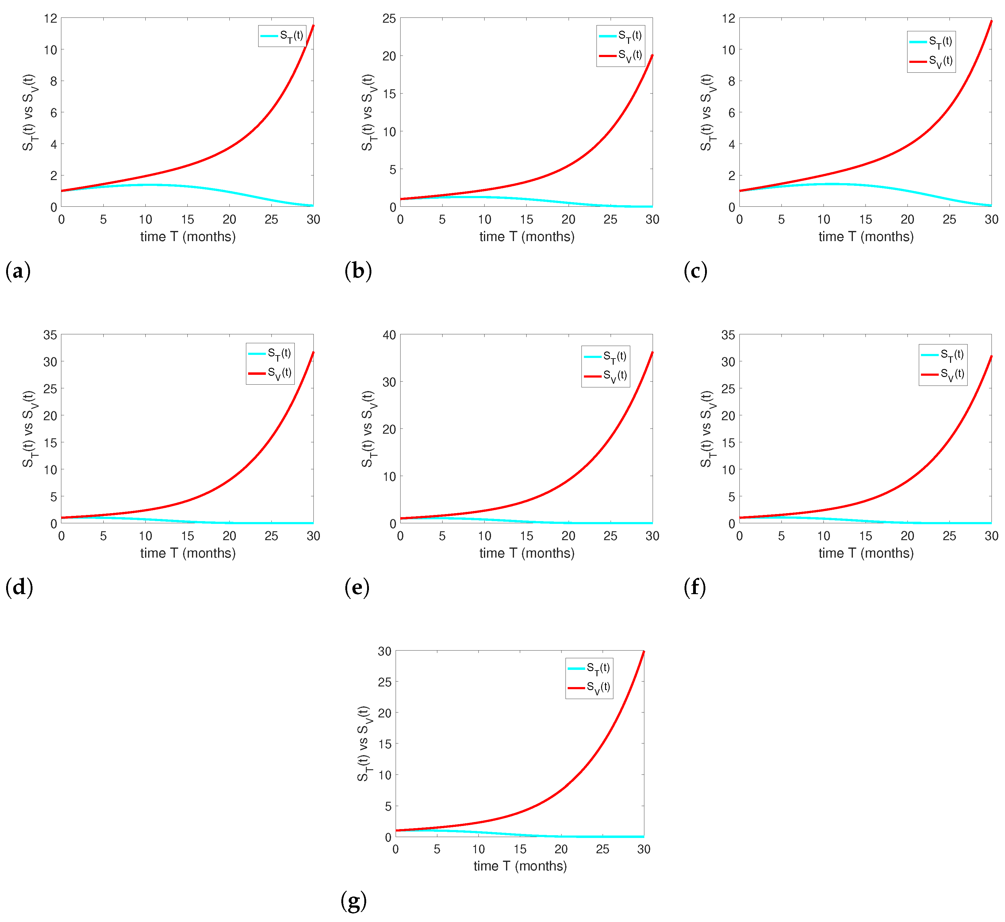
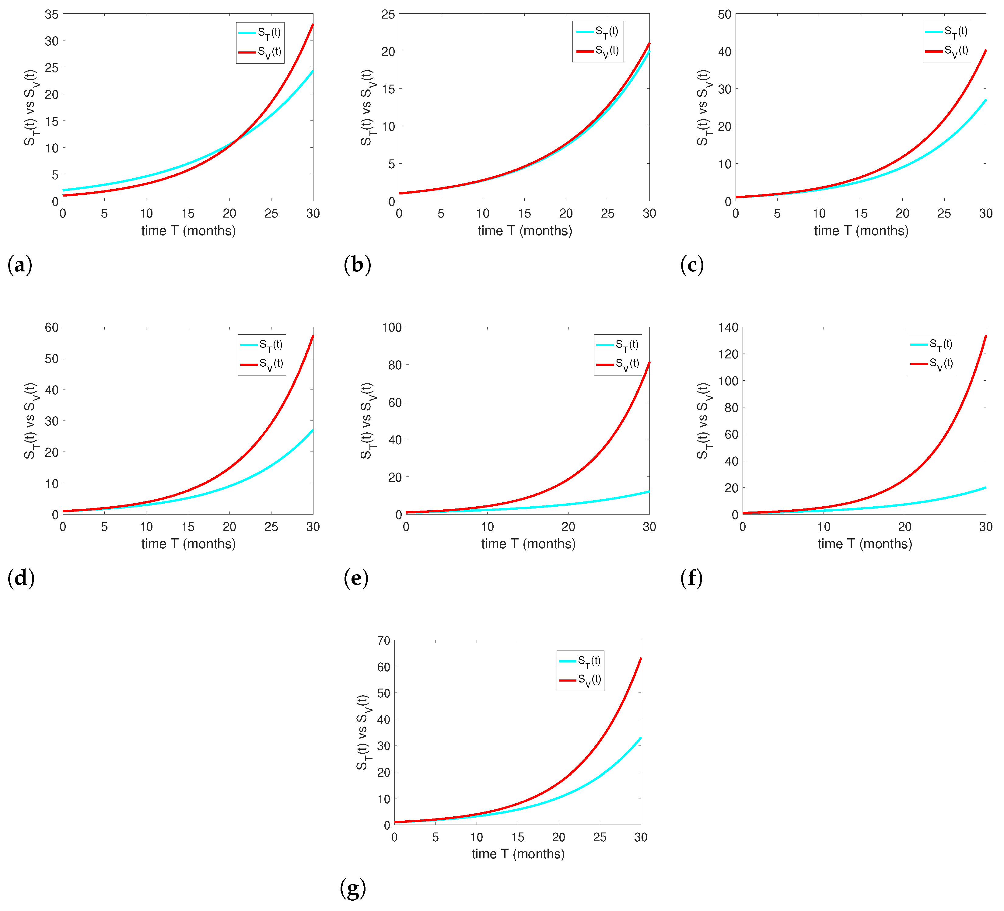
Graphical representations for Equation (1) are shown in Figure 1a–g, against the values given in Table 13. All the graphs show comparisons and competitions between the two classes of learners, who were subjected to traditional and visualized forms of learning. With the passage of time, the effectiveness of visualized modes of education will develop and be enhanced in respect to the quality of the education as well as the quantity of these learners. Their numbers or grades will increase as compared with learners who are engaged in only traditional or textual forms of learning. So, Equation (1) shows the importance and significance of the visualized forms of learning and the teachers who facilitate them. Furthermore, such education forms are necessary for all kinds of applications in various fields (technology, research, agricultural, and health industries).

Equation (2) is plotted by choosing seven different values, as given in Table 1 and Table 3, Table 4, Table 5, Table 6, Table 7 and Table 8, for $\alpha ,\beta ,\gamma$, and $\delta$, as highlighted in Table 14.

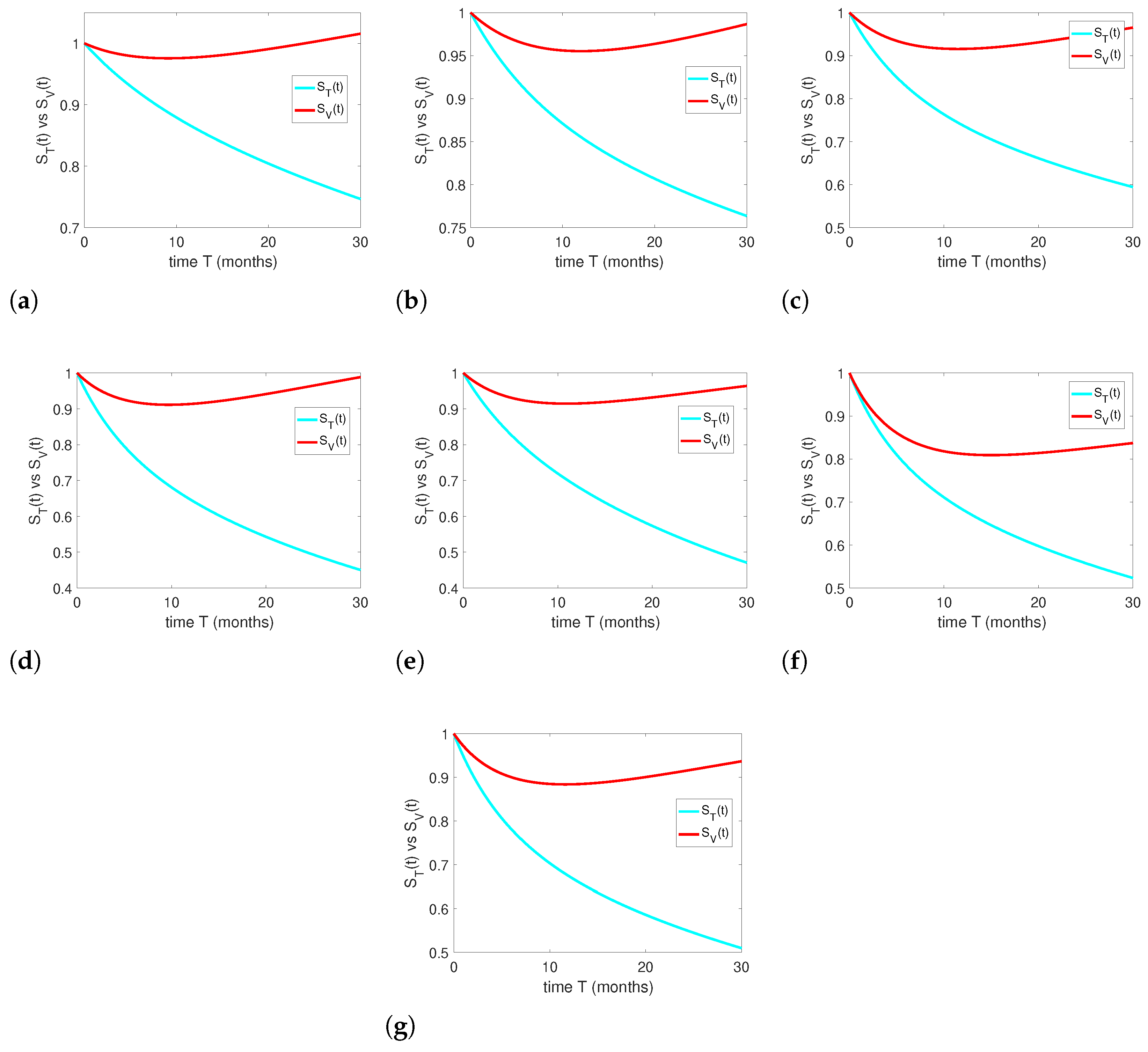
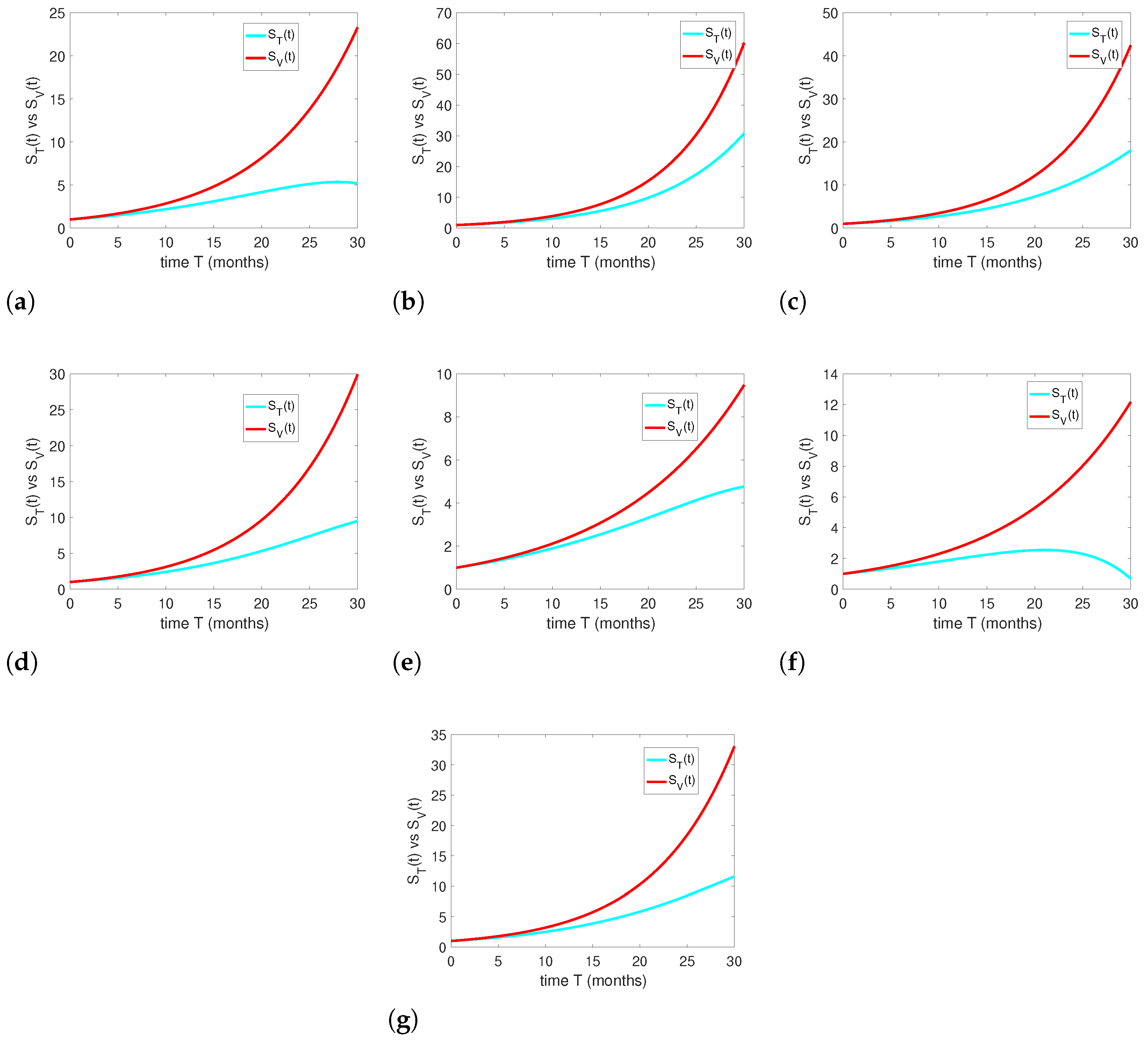
The plots used to represent Equation (2) are shown in Figure 2a–g, in comparison with the values given in Table 14. All the graphs show the comparison and competition between the two forms of learning: traditional and visualized. With the passage of time and various iterations of these learning approaches, the effectiveness of visualized education will develop in education quality and in the quantity of learners engaged in it. Their numbers or grades will also increase as compared with those attained by learners engaged in only traditional or textual forms of learning. So, Equation (2) favors learners engaged in visualized forms of learning and their teachers.

Equation (3) is plotted by choosing seven different values, as given in Table 1 and Table 3, Table 4, Table 5, Table 6, Table 7 and Table 8, for $\alpha ,\beta ,\gamma$, and $\delta$, as highlighted in Table 15.

The graphical representations for Equation (3) are shown in Figure 3a–g, against the values given in Table 15. All the graphs show the comparison and competition between the two classes of learners: only textual and visualized. With the passage of time and various iterations of these learning approaches, the effectiveness of visualized education will develop in education quality and in the quantity of learners engaged in it. So, Equation (3) also indicates that the visualized forms of learning should be implemented.

Equation (3) is plotted by choosing seven different values, as given in Table 1 and Table 3, Table 4, Table 5, Table 6, Table 7 and Table 8, for $a,a_{1}b,b_1,c,c_1$, as highlighted in Table 17.

The curves fitted for Equation (4) are shown in Figure 4a–g against the values given in Table 16. All the graphs show the comparison and competition between the two classes of learners engaged in two kinds of learning: textual and visualized. With the passage of time and various iterations of these learning approaches, the effectiveness of visualized education will develop in education quality and in the quantity of learners engaged in it; this will be reflected in learner grades and the number of learners. Equation (4) shows decay among both beginning and new learners; but with the passage of time, visualized forms of education develop and enhance student results, and is found to be effective for well-being and self-sufficient thinking among students.

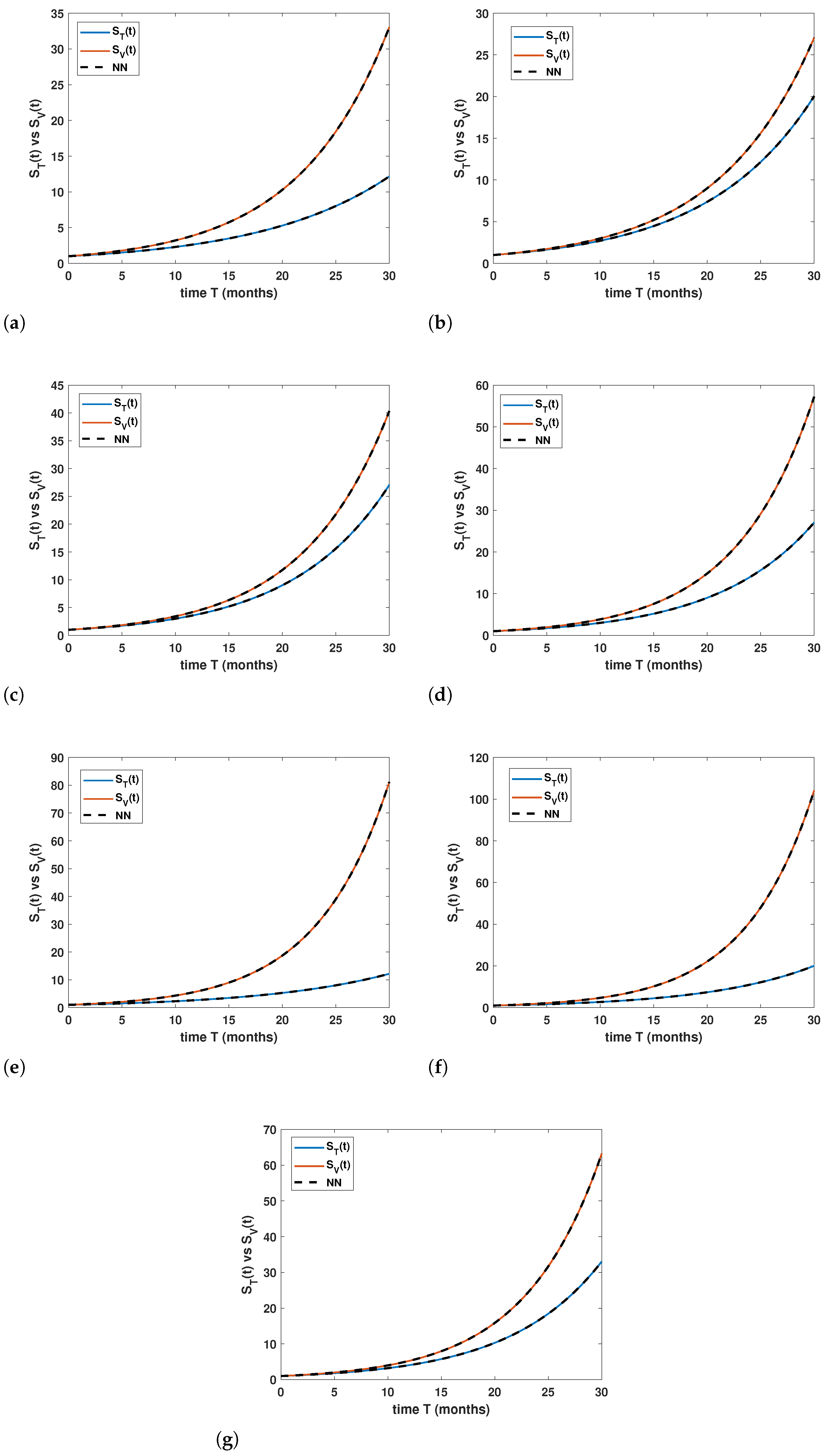
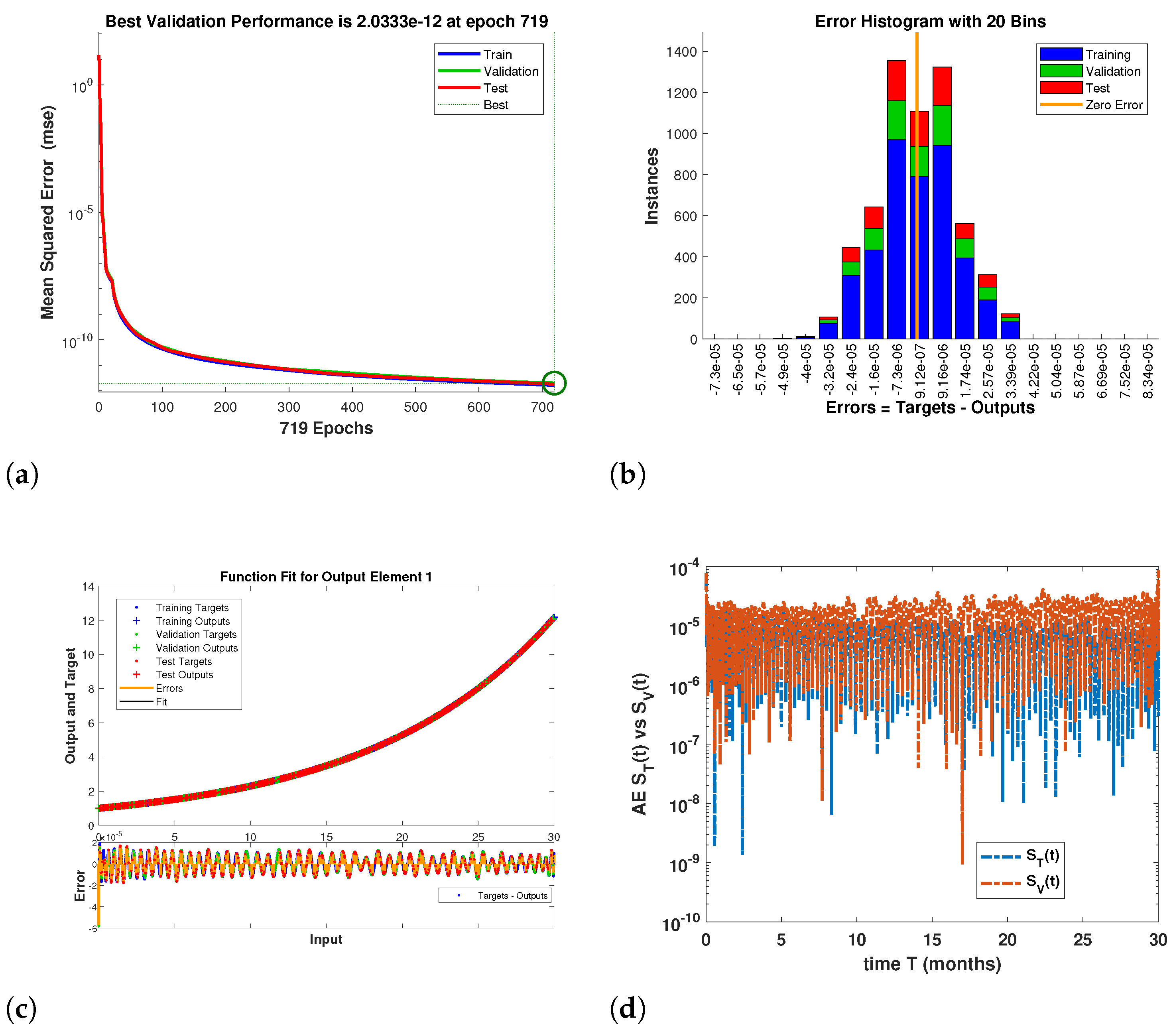
Additionally, we focused a neural network approach, Deep Neural Networks (DNNs), to test the aforementioned models. For this, the data of the random sampling and their statistics, as given in different Table 1, Table 2, Table 3, Table 4, Table 5, Table 6, Table 7, Table 8, Table 9, Table 10, Table 11, Table 12, Table 13, Table 14, Table 15, Table 16 and Table 17, were used. Furthermore, a DNN is based on multiple hidden layers; these hidden layers utilize 100 and 10 hidden neurons, accordingly. Figure 5a–g contains a comparison plot of the results with the DNN approach; one may see the best performance from the mentioned results, which is also included in the tables of random sampling. Figure 6 represents the different characteristics of the used method. Figure 6a shows that the best performance is $2.0333\times {10}^{-12}$ at epoch 719. Figure 6b represents the error histogram, with point ${9.12\times 10}^{-7}$. Figure 6c shows the fit plots for the considered model, while the absolute error of the system is presented in Figure 6d of ${10}^{-4}$. Figure 7 represents the regression of the model at approximately 1 for the training, validation, and testing data, and for all data; this verifies the accuracy of the DNN approach for the aforementioned model.

6. Conclusions

The significance of comparing different forms of education is highlighted in this study. Here, a visualized education model is compared to traditional or purely textual learning processes. Four competitive mathematical models, using the data of thirty students (data obtained through continuous random sampling experiments), have been successfully formulated. All the equations are solved by the method of decomposition, in addition to the application of Adomian polynomials for nonlinear terms. The parameters given in the mathematical models are calculated from using data gathered using sampling experiments in the form of tests. These tests were in the subject of mathematics and its six sub-branches, and they were administered to both groups of students. The first system’s numerical simulation gave the best result when it was used to compare the results from both the student groups; it was found that better grades or marks were achieved by students engaging in visualized forms of learning. This can also be seen from Table 2 and Table 9, Table 10, Table 11 and Table 12, which shows the best statistics in the post-test group. The second system is a linear competition model, with a numerical simulation which also shows the effectiveness and importance of visualized forms of learning and literacy as compared with un-visualized forms. The third system is a nonlinear competition model between the two groups; this model showed notable differences for both types of learning process. This system showed the complete superiority of the visualized learning process, with the traditional and conventional system of education being shown to be much less effective. The fourth system is a competitive model, involving logistic terms. This model points out that, when students start education with visualized forms of learning, some problems and failures will occur. However, slowly and gradually, these kinds of education will be effective and can be used to replace conventional types of learning. The four mathematical models were found to collectively favor visualized forms of education; these are supportive for future endeavors in all types of fields (technology, research, agricultural, and health industries). Furthermore, the results of random sampling, shown in the form of tables, are used for the parametrization of the four mathematical models. These are plotted across 30 months of data, with a best-fitting caparison being implemented and with the neural network being a deep neural network. The neural network was successfully used to process the training data, validation data, and testing data, as well as all the data, in the form of histogram, mean square, absolute errors, and regression analysis. This also highlighted the significant effect of visualized education forms. In the future, the models presented here could be applied in modeling competitions between two educational facilities in enrolling new students; this could be applied on a global level, with different global operators.

References

1. Yan, S.; Yang, Y. Education informatization 2.0 in China: Motivation, framework, and vision. ECNU Rev. Educ. 2021, 4, 410–428. [Google Scholar] [CrossRef]
2. Zhou, L.; Meng, W.; Wu, S.; Cheng, X. Development of Digital Education in the Age of Digital Transformation: Citing China’s Practice in Smart Education as a Case Study. Sci. Insights Educ. Front. 2023, 14, 2077–2092. [Google Scholar] [CrossRef]
3. Wang, Y.; Lin, H.; Sun, L.; Zhang, D.; Wang, J.; She, L. Research on the Deep Integration of Modern Information Technology and Five Education. In Proceedings of the 2020 International Symposium on Advances in Informatics, Electronics and Education (ISAIEE), Frankfurt, Germany, 17–19 December 2020; pp. 241–244. [Google Scholar]
4. Jacka, L. Flipping the focus: An innovative design strategy to support technology integration in teacher education. Int. J. Technol. Learn. 2023, 15, 397–411. [Google Scholar] [CrossRef]
5. Ziatdinov, R.; Valles, J.R., Jr. Synthesis of modeling, visualization, and programming in GeoGebra as an effective approach for teaching and learning STEM topics. Mathematics 2022, 10, 398. [Google Scholar] [CrossRef]
6. Nardi, E. Reflections on visualization in mathematics and in mathematics education. In Mathematics & Mathematics Education: Searching for Common Ground; Springer: Berlin/Heidelberg, Germany, 2014; pp. 193–220. [Google Scholar]
7. Presmeg, N. Visualization and learning in mathematics education. In Encyclopedia of Mathematics Education; Springer: Berlin/Heidelberg, Germany, 2020; pp. 900–904. [Google Scholar]
8. Svitek, S.; Annus, N.; Filip, F. Math Can Be Visual-Teaching and Understanding Arithmetical Functions through Visualization. Mathematics 2022, 10, 2656. [Google Scholar] [CrossRef]
9. Herrera, L.M.; Ordonez, S.J.; Ruiz-Loza, S. Enhancing mathematical education with spatial visualization tools. Front. Educ. 2024, 9, 1229126. [Google Scholar] [CrossRef]
10. Schafer, M. Manipulatives as mediums for visualisation processes in the teaching of mathematics. In Mathematics Teaching and Professional Learning in Sub-Sahara Africa; Springer: Berlin/Heidelberg, Germany, 2021; pp. 5–21. [Google Scholar]
11. Dockendorff, M.; Solar, H. ICT integration in mathematics initial teacher training and its impact on visualization: The case of GeoGebra. Int. J. Math. Educ. Sci. Technol. 2018, 49, 66–84. [Google Scholar] [CrossRef]
12. Kadunz, G.; Yerushalmy, M. Visualization in the Teaching and Learning of Mathematics. In Proceedings of the 12th International Congress on Mathematical Education: Intellectual and Attitudinal Challenges, Seoul, Republic of Korea, 8–15 July 2012; Springer International Publishing: Berlin/Heidelberg, Germany, 2015; pp. 463–467. [Google Scholar]
13. Zhang, X.; Cao, Z. A framework of an intelligent education system for higher education based on deep learning. Int. J. Emerg. Technol. Learn. 2021, 16, 233. [Google Scholar] [CrossRef]
14. Wang, R.; Daqing, G. Abnormal Behavior Recognition Algorithm in Small Sample Scenarios for a Utility Tunnel Project Based on DCGAN. J. Constr. Eng. Manag. 2025, 151, 04025043. [Google Scholar] [CrossRef]
15. Khan, Z.U.; Rahman, M.U.; Arfan, M.; Waseem; Boulaaras, S. The artificial neural network approach for the transmission of malicious codes in wireless sensor networks with Caputo derivative. Int. J. Numer. Model. Electron. Netw. Devices Fields 2024, 37, e3256. [Google Scholar] [CrossRef]
16. Saleem, A.; ur Rahman, M.; Boulaaras, S.; Guefaifia, R.; Baleanu, D. Exploring the dynamics of HIV and HCV co-infection through piecewise modified Mittag-Leffler fractional derivatives. Appl. Math. Sci. Eng. 2025, 33, 2478038. [Google Scholar] [CrossRef]
17. Waseem; Ali, S.; Rahman, M.U. Analysis of Ebola virus model using intelligent computing of a new stochastic neural network. Int. J. Biomath. 2025, 2450162. [Google Scholar] [CrossRef]
18. Faiza; Waseem; Habib, S.; Boulaaras, S.; Rahman, M.U.; Ali, S.; Alharbi, A. An Intelligent Framework for Hybrid Nanofluid Flow Between Two Concentric Cylinders Based on Deep Neural Networks. Fractals 2025, 2540182. [Google Scholar] [CrossRef]
19. He, K.; Zhang, X.; Ren, S.; Sun, J. Deep Residual Learning for Image Recognition. In Proceedings of the IEEE Conference on Computer Vision and Pattern Recognition, Las Vegas, NV, USA, 27–30 June 2016; pp. 770–778. [Google Scholar] [CrossRef]
20. Huo, Y.; Gang, S.; Guan, C. FCIHMRT: Feature Cross-Layer Interaction Hybrid Method Based on Res2Net and Transformer for Remote Sensing Scene Classification. Electronics 2023, 12, 4362. [Google Scholar] [CrossRef]
21. Samreen, A.; Baleanu, D.; Messaoudi, S.; Boulaaras, S.; Akram, S.; ur Rahman, M. Modeling the dynamics of malaria with infected immigrants using fractal–fractional techniques with deep neural networks. Asian J. Control 2025. [Google Scholar] [CrossRef]
22. Tabassum, S.; Rahman, M.U. Exploring corruption dynamics through Caputo fractional models with deep neural network interventions. J. Appl. Math. Comput. 2025, 71, 2703–2726. [Google Scholar] [CrossRef]
23. Rahman, M.U.; Boulaaras, S.; Tabassum, S.; Baleanu, D. A deep neural network analysis of fractional omicron mathematical model with vaccination and booster dose. Alex. Eng. J. 2025, 118, 435–448. [Google Scholar] [CrossRef]
24. Rahman, M.U.; Tabassum, S.; Althobaiti, A.; Waseem; Althobaiti, S. An analysis of fractional piecewise derivative models of dengue transmission using deep neural network. J. Taibah Univ. Sci. 2024, 18, 2340871. [Google Scholar] [CrossRef]
25. Silva, C.J.; Torres, D.F.M. Modeling and optimal control of HIV/AIDS prevention through PrEP. Discr. Contin. Dyn. Syst. Ser. S 2018, 11, 119–141. [Google Scholar] [CrossRef]
26. Brauer, F.; Chavez, C.C. Mathematical Models in Population Biology and Epidemiology; Springer: New York, NY, USA, 2001. [Google Scholar]
27. Diekmann, O.; Heesterbeek, J.A.P. Mathematical Epidemiology of Infectious Diseases; Wiley: New York, NY, USA, 2000. [Google Scholar]
28. He, Q.; Rahman, M.U.; Hu, J.; Cui, J. Dynamic Relationship Between Carbon Trading System Resilience and Low-Carbon Stock Market Returns Using Time-Varing Granger Causality. Fractals 2025, 15, 2540181. [Google Scholar] [CrossRef]
29. Eskandari, Z.; Avazzadeh, Z.; Ghaziani, R.K.; Li, B. Dynamics and bifurcations of a discrete-time Lotka–Volterra model using nonstandard finite difference discretization method. Math. Methods Appl. Sci. 2025, 48, 7197–7212. [Google Scholar] [CrossRef]
30. Li, B.; Liang, H.; He, Q. Multiple and generic bifurcation analysis of a discrete Hindmarsh-Rose model. Chaos Solitons Fractals 2021, 146, 110856. [Google Scholar] [CrossRef]
31. Zhang, X.; Yang, X.; He, Q. Multi-scale systemic risk and spillover networks of commodity markets in the bullish and bearish regimes. N. Am. J. Econ. Financ. 2022, 62, 101766. [Google Scholar] [CrossRef]
32. Hale, J.K. Ordinary Differential Equations; Dover Publications: New York, NY, USA, 2009. [Google Scholar]
33. Hartman, P. Ordinary Differential Equations, Classics in Applied Mathematics, 2nd ed.; Society for Industrial and Applied Mathematics: Philadelphia, PA, USA, 2002. [Google Scholar]
34. Hirsch, M.W. Systems of differential equations which are competitive or cooperative IV: Structural stability in three dimensional systems. SIAM J. Math. Anal. 1990, 21, 1225–1234. [Google Scholar] [CrossRef]
35. Grassly, N.C.; Fraser, C. Mathematical models of infectious disease transmission. Nat. Rev. Microbiol. 2008, 6, 477–487. [Google Scholar] [CrossRef]
36. Guo, H.; Li, M. Global dynamics of a staged progression model for infectious diseases. Math. Biosci. Eng. 2006, 3, 513–525. [Google Scholar] [CrossRef] [PubMed]
37. Zill, D.G. Differential Equations with Boundary-Value Problems, 9th ed.; Cengage Learning: Boston, MA, USA, 2016; ISBN 1305965795/978-1305965799. Available online: https://books.google.com/books?id=Mui5DQAAQBAJ (accessed on 23 August 2025).
Figure 1. Comparison between traditional, S T ( t ) , and visualized, S V ( t ) , forms of learning. Equation (1) used to obtain the seven different values of the given parameters.
Mathematics 13 02793 g001
Figure 2. Comparison between traditional, S T ( t ) , and visualized, S V ( t ) , forms of learning. Equation (2) was used to obtain the seven different values of the given parameters.
Mathematics 13 02793 g002
Figure 3. Comparison between traditional, S T ( t ) , and visualized, S V ( t ) , forms of learning. Equation (3) was used to obtain the seven different values of the given parameters.
Mathematics 13 02793 g003
Figure 4. Comparison between traditional, S T ( t ) , and visualized, S V ( t ) , forms of learning. Equation (4) was used to obtain the seven different values of the given parameters.
Mathematics 13 02793 g004
Figure 5. Neural network approach of traditional, S T ( t ) , and visualized, S V ( t ) , forms of learning. Equation (4) was used to obtain the different seven values of the given parameters.
Mathematics 13 02793 g005
Figure 6. Neural-network-based plots for traditional, S T ( t ) , and visualized, S V ( t ) , forms of learning. Equation (4) was used. (a) Performance; (b) histogram; (c) fit; (d) absolute error.
Mathematics 13 02793 g006
Figure 7. Regression diagram of for traditional, S T ( t ) , and visualized, S V ( t ) , forms of learning. According to Equation (4).
Mathematics 13 02793 g007