Article

A Kinetic Theory Approach to Modeling Counterflow in Pedestrian Social Groups †

1
Laboratory of Applied Mathematics and Computer Science, Faculty of Sciences and Technologies of Marrakech, Cadi Ayyad University, Marrakech 40000, Morocco
2
EFREI Research Lab, Université Paris-Panthéon-Assas, 30/32 Avenue de la République, 94800 Villejuif, France
*
Author to whom correspondence should be addressed.
To the memory of Professor Abdelghani Bellouquid.
Mathematics 2025, 13(17), 2788; https://doi.org/10.3390/math13172788 (registering DOI)
Submission received: 29 July 2025 / Revised: 19 August 2025 / Accepted: 22 August 2025 / Published: 30 August 2025
(This article belongs to the Section E4: Mathematical Physics)

Abstract

This article focuses on modeling counterflows within pedestrian social groups in a corridor using the kinetic theory approach, specifically when two social groups move in opposite directions. The term social group refers to a set of pedestrians with established social relationships who stay as close as possible to one another and share a common goal or destination, such as friends or family. The model accounts for interactions both within the same social group and between pedestrians from different social groups. Numerical simulations based on a Monte Carlo particle method are performed. A key criterion for evaluating simulation models is their ability to reproduce empirically observed collective motion patterns. One of the most significant emergent behaviors in bidirectional pedestrian flows is lane formation. To analyze this phenomenon, we employ Yamori’s band index to quantify the evolution of lane structures.

1. Introduction

Modeling and simulations of pedestrian dynamics, viewed as a living system, have attracted significant attention from researchers and policymakers due to their vital role in crowd safety and their broader impact on societal well-being. These models provide insights into human movement patterns, aiding in the development of safer urban infrastructure, efficient evacuation strategies, and optimized public spaces [1,2]. Furthermore, simulations help predict risks in high-density areas, support emergency decision-making, and contribute to the design of adaptive transportation systems that improve mobility and safety [3,4].
Mathematical models of pedestrian dynamics are commonly categorized into three modeling scales: microscopic, which focuses on individual-based interactions [5]; macroscopic, which describes crowd movement using hydrodynamic principles [6]; and mesoscopic, an intermediate scale based on generalized kinetic theory approaches [3]. The reader is referred to [4,7] for recent discussions on the topic.
The dynamics of living particles, such as pedestrians in a crowd, differ significantly from those of inert systems because they involve perception, decision-making, and adaptive behavior [8,9]. Traditional physical models based on conservation laws and equilibrium equations may not fully capture the complexity of human movement. Unlike inert particles, pedestrians anticipate obstacles, interact socially, and adjust their trajectories based on their goals and surroundings, making their mathematical modeling significantly more challenging [3,4]. Therefore, modeling pedestrian dynamics requires approaches that incorporate elements of living systems, such as cognition, learning, and collective movement dynamics [9].
The kinetic theory of active particles models pedestrians as active particles characterized by heterogeneous abilities and strategies [3,4]. Their microscopic state includes mechanical variables such as position and velocity, along with a behavioral variable termed “activity,” representing their social–emotional state such as stress [8,10], emotional contagion [11], and learning level [12]. This refined modeling approach captures the unique behaviors and interactions of pedestrian systems, bridging the gap between the mathematics of inert matter and the complexities of pedestrian dynamics [4,9]. It has been widely applied to developing models for various complex living systems, including cancer dynamics [13], epidemiological models [14], and vehicular traffic [15].
Bellomo et al. introduced a kinetic model of crowd behavioral dynamics in [16,17]. It was later applied in [11,18,19,20,21] to simulate the evacuation of different groups in complex geometries and to compute evacuation times from venues with internal obstacles. Further advancements were made in two works [12,22]. The work of [22] develops a kinetic model that incorporates a stress-level parameter to capture pedestrians’ adaptive behavior in emergency situations. A data-driven inverse problem approach is used to estimate this parameter, ensuring accurate modeling of crowd responses under stress. The work of [12] explores crowd evacuation dynamics involving leaders and followers. Recent studies have focused on understanding the behavioral and social dynamics of crowds. For example, a kinetic model was developed to simulate crowd dynamics, considering stress conditions, boundary conditions, and safety concerns [8,10]. Additionally, Bellomo et al. explored emergent behaviors in crowds, highlighting the influence of emotional states on overall crowd dynamics [3,4,11,18,23] (see also [5,6], which focus on improving crowd dynamics models by incorporating the evolving psychological states of pedestrians). In light of the COVID-19 pandemic, several studies in [24,25,26] have investigated the early transmission of highly infectious diseases through social interactions. These contributions utilize a coupled approach, integrating a kinetic model of crowd dynamics with a contagion model.
Most kinetic models traditionally represent a crowd as a collection of isolated individuals. However, in reality, pedestrians often move in social groups, as discussed in [2,27,28,29]. In this paper, a “social group” refers to a set of pedestrians with varying social relationships who remain close to each other and share a common goal or purpose [27,28]. Understanding the impact of social grouping is crucial, as it significantly influences the dynamics of pedestrian crowds [29,30,31]. Indeed, various computational models, including cellular automata [32,33], agent-based models [34,35], and social force models [36] are commonly used to simulate group movement. A flexible approach has been introduced to model social groups with leadership roles [37], while social force models have been applied to study pedestrian social group evacuations [1,29,38,39,40]. Recent advancements have introduced a 2D mesoscopic model in [41], which excels in incorporating interactions with walls, exits, and obstacles, offering a more detailed and realistic representation of pedestrian social group behavior compared to traditional models.
In this work, we extend our kinetic-type model, which was recently introduced in [41], to model the dynamics of social group counterflows in corridors under stressful conditions. A pedestrian social group is a complex system, which can perform various self-organization phenomena [1,2]. Thus, a commonly used method to evaluate the performance of pedestrian social group simulation models is to reproduce the emergence of empirically observed collective patterns of motion [2,4]. The formation of pedestrian social group lanes in the bidirectional pedestrian flow is one of the most important phenomena, where individuals avoid moving pedestrians in the counterflow and share the available space by forming lanes of uniform moving directions [30,42]. To better describe the evolution of lane formation in bidirectional pedestrian flow, Yamori’s band index is employed in this study [18,43].
The rest of this paper is organized as follows: Section 2 introduces the mathematical kinetic model for pedestrian social group counterflows in a corridor. Section 3 provides a detailed description of interactions both within the same social group and between different social groups. In Section 4, we first briefly describe the principles of the numerical method, which is based on the Monte Carlo technique, followed by the presentation of numerical results. Finally, Section 5 discusses the limitations of this study and presents further research directions.

2. The Mathematical Model of the Pedestrian Social Group

This section introduces the kinetic modeling of counterflows in pedestrian social groups, beginning with an overview of the variables and parameters that define the model. The problem is framed within the context of social group dynamics, with a particular focus on the counterflow of social groups within a corridor. The mesoscopic description captures the collective behavior of pedestrian groups, from which macroscopic quantities, such as group density and mean velocity, are derived. Finally, the mathematical structure of the proposed model is presented.

2.1. Variables and Parameters of the Model

We consider the dynamics in a two-dimensional domain, denoted by Ω , within which the crowd moves. The region containing the entire crowd at the initial time is represented by Ω 0 Ω [4]. The diameter of the circle enclosing Ω is denoted by L.
The microscopic state of each pedestrian includes the following:
  • The position x = ( x , y ) .
  • The velocity v , which is expressed in polar coordinates as
    v = v cos θ , sin θ ,
    where v represents the speed and θ denotes the velocity direction.
We define the velocity space as
V = ( v , θ ) v V m , θ [ 0 , 2 π ) ,
where V m represents the maximum velocity that a fast-moving pedestrian can attain under free-flow conditions [41].
As discussed in [4], we introduce the parameter α [ 0 , 1 ] , which models the quality of the environment, including factors such as the presence of smoke or weather conditions, where
  • α = 1 represents the best-quality domain.
  • α = 0 denotes to the worst-quality domain.
Remark 1.
Dimensionless quantities are introduced by normalizing all linear spatial components with a characteristic length L, all velocities with the maximum speed V m , and time t with the characteristic time T r , defined as T r = L / V m . Consequently, all physical quantities are scaled to the range [ 0 , 1 ] .

2.2. Position of the Problem Under Study

We consider two social groups moving in opposite directions, each composed of several nearby pedestrians who seek to stay together while attempting to reach their respective targets. To model the decision-making of each group, we introduce the variable u, which represents the group’s preferences.
Let I u = { u 1 , u 2 } denote the set of admissible discrete values of the variable u such that
  • u 1 represents the social group choosing to move to the right.
  • u 2 represents the social group choosing to move to the left.
For simplicity,
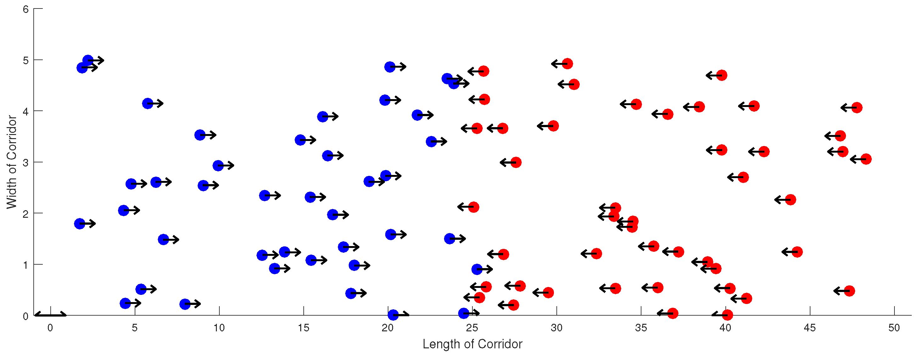
  • The social group moving to the right (depicted in blue) is identified as the first social group (see Figure 1).
  • The social group moving to the left (depicted in red) is referred to as the second social group (see Figure 1).
This setup reflects a counterflow situation, which is commonly observed in pedestrian dynamics, where individuals with opposing movement intentions coexist within the same spatial domain. Accordingly, the system is divided into two social groups, each associated with a distinct direction of movement (left or right). We refer to each social group as a functional subsystem.
Figure 1. Schematic illustration of pedestrian social groups in counterflow within a straight corridor. The first social group (blue) chooses to move to the right, while the second social group (red) chooses to move to the left.
Mathematics 13 02788 g001
Remark 2.
It should be noted that the variable u is a deterministic variable, which represents the movement preference of each social group. It should not be confused with the activity variable discussed in [3], which pertains to a different aspect of pedestrian behavior.

2.3. The Mesoscopic Description and Macroscopic Observable Quantities

The mesoscopic description of the overall system is delivered by the statistical distribution at time t over the following microstate:
f ( t , x , v , u ) = i = 1 2 f t , x , v , u i δ u u i = i = 1 2 f i ( t , x , v ) δ u u i ,
where f i ( t , x , v ) : = f ( t , x , v , u i ) for each functional subsystem labeled by i = 1 , 2 .
Remark 3.
In Equation (1), δ ( u u i ) is a Dirac delta function used to represent the discrete choice of movement direction ( u 1 or u 2 ) for each social group.
If f i is locally integrable, then f i t , x , v d x d v represents the (expected) infinitesimal number of pedestrians of the i-th social group, which is at the instant t in the elementary volume [ x , x + d x ] × [ v , v + d v ] with x Ω and v V .
For i 1 , 2 , the probability distributions f i are normalized by ρ max , which defines the maximal full packing density of pedestrians.
Remark 4.
It is worth mentioning that the maximal density of pedestrians, ρ max , is approximately 7 p e d / m 2 [44].
Under integrability conditions, velocity-weighted moments of f i lead to the computation of macroscopic observable quantities. For instance, the local density and mean velocity for each i-th social group are given as follows:
ρ i t , x = V f i t , x , v d v , i = 1 , 2 ,
and
ξ i t , x = 1 ρ i ( t , x ) V v f i t , x , v d v , i = 1 , 2 .
Global expressions are obtained as a weighted sum over the index labeling the social groups; that is,
ρ ( t , x ) = i = 1 2 ρ i ( t , x ) ,
and
ξ ( t , x ) = 1 ρ ( t , x ) i = 1 2 ρ i ( t , x ) ξ i ( t , x ) .

2.4. Mathematical Structure

The model presented in [41] is revisited to streamline its mathematical formulation while also evaluating its effectiveness in modeling counterflow within social groups. To achieve this, the mathematical framework is based on an integro-differential equations system designed to describe the time evolution of the distribution functions f i . These functions can be derived from a particle balance in the elementary volume of the microstate space [3,4]. The conservation law can be expressed in the following form, as shown in [18]:
Variation rate of the number of active particles = Inlet flux rate Outlet flux rate ,
where the inlet and outlet fluxes are due to interactions. This equation refers to the following structure:
t + v · x f i ( t , x , v ) = η i V P i [ ρ i , ξ i ] v v f i t , x , v d v f i ( t , x , v ) + μ i V T i [ ρ , ξ ] v v f i t , x , v d v f i ( t , x , v ) i = 1 , 2 ,
where
  • t denotes the partial derivative with respect to time t.
  • x denotes the gradient operator with respect to the spatial variable x . Consequently, v · x represents the transport operator along the velocity vector v .
  • η i is the interaction rate between pedestrians of the same i-th social group, representing the frequency of binary encounters per unit time. In this paper, we assume that it is constant.
    η i = η 0 .
  • P i [ ρ i , ξ i ] v v is the velocity transition probability density, which models the dynamics by which pedestrians in the same i-th social group adjust their velocity due to interactions with other walkers in the same group.
  • μ i is the interaction rate between pedestrians of the i-th social group and pedestrians from other social groups. In this paper, we assume that it is constant.
    μ i = μ 0 .
  • T i [ ρ , ξ ] v v is the velocity transition probability density that models the dynamics by which pedestrians of the i-th social group modify their velocity due to interactions with pedestrians from other social groups.
The terms P i [ ρ i , ξ i ] v v and T i [ ρ , ξ ] v v are explained in detail in the following section.
Remark 5.
In Equation (4), square brackets are used to indicate the functional dependence of the transition probability density T i on the density ρ and mean velocity ξ, while the transition probability density P i depends on the local density ρ i and local mean velocity ξ i of the i-th social group.
Remark 6.
In [3,18], the modification to account for the change in direction for pedestrians is included in the transition probability density, while in this present model, it is additive. Indeed, the transition probability density in our model can be viewed as the sum of two contributions, with the former modeling interactions between walkers of the same social group and the second modeling interactions between walkers of the same social group with other social groups.

3. Toward Modeling Interactions

This section highlights the development of interaction modeling, a crucial component that significantly impacts the effectiveness of the model. To this end, we drew inspiration from previous models presented in [3,4,11,18,41].
As outlined in Refs. [4,11,41], the foundational assumptions for interaction modeling are as follows:
  • We assume that the interactions between pedestrians within a social group influence their dynamics in the following ways [41]:
    • First, by altering their direction of movement, denoted as θ .
    • Second, by changing their velocity modulus, v.
  • All pedestrians within a social group are influenced by various stimuli, including (a) rational movement, which refers to the tendency to move toward a target while avoiding crowded areas, and (b) irrational movement, such as being drawn to the main flow due to stress-induced behavior [3,4].
  • The selection of the velocity direction θ corresponds to a weighted selection of the stimuli mentioned in Item 2, depending on the quality of the venue α , the level of stress, and the density [18,41].
  • Once a walking direction has been selected, each pedestrian in a social group adjusts their speed to the mean speed and density, also depending on the venue quality parameter α and the level of stress [41].
  • Following [11,41], the heuristic modeling of speed dynamics is based on the reasoning that if a pedestrian’s speed is less than (greater than) the average speed, they tend to increase (decrease) their speed; this is guided by a decision process influenced by low perceived density and the overall quality of the environment.
As discussed in [3,4], we introduce the parameter β , which models the stress level of pedestrians within the same social group. For i { 1 , 2 } , the stress level β i [ 0 , 1 ] for the i-th social group is defined as follows:
  • β i = 1 refers to the highest level of stress.
  • β i = 0 refers to the lowest level of stress.
Remark 7.
It should be noted that the stress level β i is a scalar variable that is uniformly shared by all pedestrians within the same i-th social group and remains unaffected by interactions [18,41].
This section begins by addressing the interactions within the same social group and then extends to the interactions between pedestrians from different social groups.

3.1. Modeling Interactions Between Walkers of the Same Social Group

It is assumed that interactions among walkers in the same i-th social group first affect their movement direction, then their speed. Thus, the transition probability density P i [ ρ i , ξ i ] v v can be factorized as follows:
P i [ ρ i , ξ i ] v v = P i [ ρ i , ξ i ] v v P i [ ρ i , ξ i ] θ θ ,
where the velocity is separated into speed and direction components v = { v , θ } .
The terms P i [ ρ i , ξ i ] v v and P i [ ρ i , ξ i ] θ θ are explained in detail in the following section.

3.1.1. Selection of the Direction of Movement

Adjustment of walking direction by pedestrians of the same i-th social group is assumed to be influenced by three stimuli [3,41], which are
  • The trend towards a defined target. This direction is represented by the unit vector v ( t a r g e t ) .
  • The desire to avoid overcrowded areas. This direction is represented by the unit vector v ( v a c u u m ) , with
    v ( v a c u u m ) = x ρ i | | x ρ i | | ,
    where ρ i is the density given by (2).
  • The attraction to the mean stream. This direction is represented by the unit vector v ( s t r e a m ) , with
    v ( s t r e a m ) = ξ i | | ξ i | | ,
    where ξ i is the mean velocity of the i-th social group given by (3) and ξ i is the mean speed.
Remark 8.
v ( v a c u u m ) is a unit vector directed away from the regions of the highest density, representing an effort to evade congestion by moving toward areas with lower density. (see Figure 2).
In high-density situations, pedestrians of the same i-th social group attempt to avoid the most overcrowded areas by moving in the direction of v ( v a c u u m ) . Conversely, at low density, pedestrians head toward a target, v ( t a r g e t ) , unless their stress level is high, in which case they tend to follow the mean flow as represented by v ( s t r e a m ) . According to [3,4,41], the desired direction is defined as follows:
v ( p ) = ρ i v ( v a c u u m ) + ( 1 ρ i ) β i v ( s t r e a m ) + ( 1 β i ) v ( t a r g e t ) β i v ( s t r e a m ) + ( 1 β i ) v ( t a r g e t ) ρ i v ( v a c u u m ) + ( 1 ρ i ) β i v ( s t r e a m ) + ( 1 β i ) v ( t a r g e t ) β i v ( s t r e a m ) + ( 1 β i ) v ( t a r g e t ) .
The transition probabilities for angles read as follows:
P i [ ρ i , ξ i ] θ θ ; β i = δ θ θ ( p ) [ ρ i , ξ i ] ,
where the preferred angle θ ( p ) can be obtained from Equation (8) by using the following relation:
v ( p ) = cos θ ( p ) , sin θ ( p ) .

3.1.2. Adjustment of the Speed to Local Conditions

As for speed, the kinetic theory approach accounts for the perceived density ρ θ along the direction θ , as defined in [18], as follows:
ρ θ [ ρ ] = ρ + θ ρ 1 + θ ρ 2 ( 1 ρ ) H θ ρ + ρ H θ ρ ,
where
  • θ denotes the derivative along the direction θ .
  • H ( · ) is the Heaviside function, with H ( · 0 ) = 1 and H ( · < 0 ) = 0 .
Remark 9.
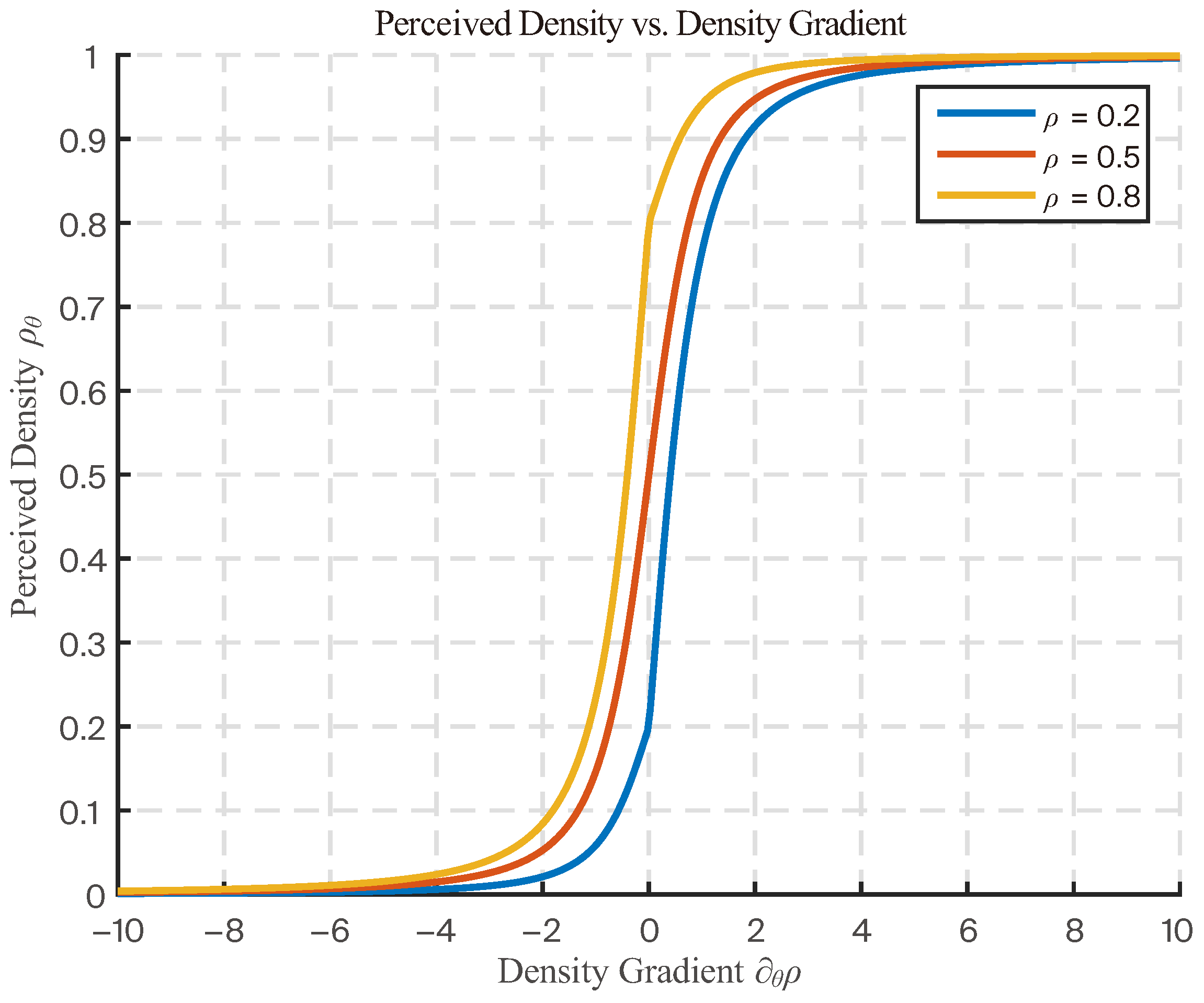
As a result of Equation (10), positive gradients cause the perceived density to increase up to a maximum value of ρ θ = 1 , while negative gradients cause it to decrease to a minimum value of ρ θ = 0 , as shown in Figure 3, and they are expressed in the following way:
θ ρ ρ θ 1 , θ ρ = 0 ρ θ = ρ , θ ρ ρ θ 0 .
After selecting the velocity direction, pedestrians of the same i-th social group adjust their speed based on the local density ρ i and local mean velocity ξ i . According to [11,41], two cases are distinguished:
  • The speed of each walker of the i-th social group is lower than the local mean speed of the i-th social group | | ξ i | | . The walker of the i-th social group either maintains their speed or accelerates to a speed of v a i , which increases as local density becomes lower [41]. It is reasonable to assume that the probability to accelerate, p a i , decreases with the congestion of the space and with the badness of the environmental conditions [11].
  • The speed of each walker of the i-th social group is greater than or equal to the local mean speed | | ξ i | | . The walker of the i-th social group either maintains their speed or decelerates to a speed of v d i , which lowers as local density becomes higher [41]. It is reasonable to assume that the probability to decelerate, p d i , increases with the congestion of the space and the goodness of the environmental conditions [11].
Therefore, the transition probability density for speed can be expressed as follows:
P i [ ρ i , ξ i ] v v = p a i δ v v a i + 1 p a i δ v v if | | ξ i | | v p d i δ v v d i + 1 p d i δ v v otherwise
where
v a i = | | ξ i | | + λ i 1 ρ θ ( p ) [ ρ i ] λ i | | ξ i | | ,
p a i = λ i 1 ρ θ ( p ) [ ρ i ] ,
v d i = 1 ρ θ ( p ) [ ρ i ] | | ξ i | | ,
and
p d i = ρ θ ( p ) [ ρ i ] 1 λ i C 1 .
In Equations (12)–(15), ρ θ ( p ) [ ρ i ] is the perceived density, as given by Equation (10), along the preferred walking direction θ ( p ) , λ i = α β i , and the constant C 1 < 1 is introduced in order to take into account that the probability to decelerate is not naught even if λ i = 1 [41].
The main features of the transition probability densities P i [ ρ i , ξ i ] v v are summarized in Table 1.
Remark 10.
In [3,18], walkers interact with all others in their visibility domain, but in the present paper, we assumed that their mutual interactions depend only on the local density and mean velocity. This modeling strategy facilitates the formulation of a computational model that drives efficient numerical simulations while maintaining a sufficient description of the dynamics of the crowd [41].

3.2. Modeling Interactions Among a Social Group and Other Social Groups

It is assumed that interactions between walkers belonging to the i-th social group and those from other social groups primarily involve changes in their movement direction, followed by modifications to their speed [41]. Therefore, the transition probability density can be factorized as follows:
T i [ ρ , ξ ] v v = T i [ ρ , ξ ] v v T i θ θ .

3.2.1. Selection of the Direction of Motion

The transition probabilities for angles read as follows:
T i θ θ = δ θ θ ( t a r g e t ) ,
where θ ( t a r g e t ) represents the velocity direction of v ( t a r g e t ) .
Remark 11.
θ ( t a r g e t ) in our model corresponds to the desired movement direction of the pedestrians. For example, the first social group moves to the left, while the second social group moves to the right.

3.2.2. Adjustment of the Speed to Local Conditions

According to [11,41] two cases are distinguished:
  • The speed of each walker of the i-th social group is lower than the global mean speed | | ξ | | . The walker of the i-th social group either maintains their speed or accelerates to a speed of v a c i which is becomes higher as density becomes lower [41]. It is reasonable to assume that the probability to accelerate, r a i , decreases with the congestion of the space and with the badness of the environmental conditions [11].
  • The speed of each walker of the i-th social group is greater than or equal to the global mean speed | | ξ | | . The walker of the i-th social group either maintains their speed or decelerates to a speed of v d e i , which becomes much lower as density becomes higher [41]. It is reasonable to assume that the probability to decelerate, r d i , increases with the congestion of the space and the goodness of the environmental conditions [11].
Thus, the transition probability density for the speed can be expressed as follows:
T i [ ρ , ξ ] v v = r a i δ v v a c i + 1 r a i δ v v if | | ξ | | v r d i δ v v d e i + 1 r d i δ v v else
where
v a c i = | | ξ | | + α 1 ρ θ ( t a r g e t ) [ ρ ] α | | ξ | | ,
r a i = α 1 ρ θ ( t a r g e t ) [ ρ ] ,
v d e i = 1 ρ θ ( t a r g e t ) [ ρ ] | | ξ | | ,
and
r d i = ρ θ ( t a r g e t ) [ ρ ] 1 α C 2 .
In Equations (19)–(22), ρ θ ( t a r g e t ) [ ρ ] is the perceived density, as given by Equation (10), along the preferred walking direction θ ( t a r g e t ) , and the constant C 2 < 1 is introduced in order to take into account that the probability to decelerate is not naught even if α = 1 [41].
The main features of the transition probability densities T i [ ρ , ξ ] v v are summarized in Table 2.
The kinetic model: The interaction rates defined by Equations (5) and (6), along with the model’s partial differential equation (Equation (4)) and the initial conditions f 0 i ( x , v ) for i { 1 , 2 } , allow the derivation of the mathematical model:
t + v · x f i ( t , x , v ) = η 0 V P i [ ρ i , ξ i ] v v f i t , x , v d v f i ( t , x , v ) + μ 0 V T i [ ρ , ξ ] v v f i t , x , v d v f i ( t , x , v ) , f i ( 0 , x , v ) = f 0 i ( x , v ) , x Ω , v V ,
where P i [ ρ i , ξ i ] v v is defined by Equation (7) and T i [ ρ , ξ ] v v is defined by Equation (16).

4. Results and Numerical Simulations

In this section, we begin by briefly describing the principles of the numerical method, which is based on the Monte Carlo technique. Then, the numerical results are presented.

4.1. Description of the Numerical Method

Kinetic crowd models have been solved numerically using both deterministic and stochastic methods [4,41]. Deterministic methods include the finite difference method [12,19,21] and the finite volume method [20], while stochastic methods such as the Monte Carlo method have also been employed [8,11,18,23,41].
In this work, the Monte Carlo particle scheme has been adopted and further developed. Compared to deterministic solution methods, this stochastic approach offers several attractive features that make it one of the most popular and widely used simulation techniques for solving kinetic crowd models. These features include the ability to handle large crowd sizes efficiently, ease of managing complex geometries, and suitability for high-performance computing, which helps maintain computational times that are shorter than the actual simulated time [8,11,18,41]. Additionally, the method facilitates the modeling of complex interaction rules between pedestrians [10] and effectively accounts for varying stress levels within the crowd [11].
The most widely used strategy consists of decoupling the transport and interaction (collision) terms by time-splitting the evolution operator into a drift step, in which collisions are neglected, and a collision step, in which there is no spatial motion [45]. Indeed, a large number of simulated particles whose positions and velocities evolve over time by a sequence of time steps are used to represent the distribution function f i for i { 1 , 2 } . Each time step consists of a drift and a collision sub-steps.
The former corresponds to the streaming operator on the left-hand side of Equation (4), whereas the latter is performed according to stochastic rules, consistent with the structure of the interaction terms on the right-hand side of Equation (4) and the transition probability densities given by Equations (9), (11), (17), and (18). The main algorithm is summarized in Algorithm 1.
The space domain to be simulated is partitioned into a finite number of disjoint cells. These cells are used for the sampling of macroscopic properties such as mean velocity and density [45]. Valuable references are provided by the standard books [45,46], as well as the references therein.
Finally, the implementation of the Monte Carlo algorithm was carried out using Python 3.11 on a computer equipped with an Intel® Core™ i7 processor and 16 GB of RAM, running Windows 10. The visualization of simulation results was performed using Matplotlib 3.7.2 on the same computing environment.

4.2. Simulation of Bidirectional Pedestrian Social Group Flow

Pedestrian social groups are complex systems capable of exhibiting various self-organizing behaviors [1,2,47]. A widely accepted approach for evaluating the performance of pedestrian simulation models is to test their ability to reproduce empirically observed collective motion patterns [2,4]. Validation is typically carried out either by comparing simulation results with experimental data—many of which are publicly accessible (e.g., in the archive [48])—or by checking whether certain emergent qualitative behaviors observed in real crowds are faithfully reproduced [4,18].
One of the most prominent emergent phenomena in bidirectional pedestrian flow is the spontaneous formation of lanes, where individuals moving in opposite directions segregate and share the available space efficiently [18]. In this part, we focus on reproducing this well-documented behavior to assess the model’s ability to capture lane formation dynamics. The main objective of the simulations is to demonstrate the spontaneous segregation of pedestrians into lanes with uniform walking directions.
Algorithm 1 The Monte Carlo algorithm with splitting
 1: Input: N particles per social groups, time step Δ t , initial distribution f i 0 ( x , v ) for i = 1 , 2
 2: Initialize: For each social groups i = 1 , 2 , sample { ( x j ( i ) , v j ( i ) ) } j = 1 N from f i 0 ( x , v )
 3: for each time step t t + Δ t  do
 4:      // Transport Step
 5:      for each social groups i = 1 , 2  do
 6:           for each particle j = 1 to N do
 7:                 x j ( i ) x j ( i ) + Δ t · v j ( i )
 8:                Apply boundary conditions to x j ( i ) if needed
 9:             end for
10:      end for
11:      // Interaction or Collision Step
12:      for each social groups i = 1 , 2  do
13:            Estimate local density ρ i ( x ) and other parameters ξ i
14:            for each particle j = 1 to N do
15:               Sample r U [ 0 , 1 ]
16:               if  r < η 0 η 0 + μ 0  then
17:                 // P-type interaction
18:                 Randomly select particle m { 1 , , N }
19:                 Sample v new P i [ ρ i , ξ i ] ( v m ( i ) v )
20:               else
21:                 // T-type interaction
22:                 Randomly select particle m { 1 , , N }
23:                 Sample v new T i [ ρ , ξ ] ( v m ( i ) v )
24:               end if
25:                v j ( i ) v new
26:            end for
27:      end for
28:   end for
The Yamori band index [43] and the order parameter [49] are essential metrics for analyzing self-organization in bidirectional pedestrian flow. The Yamori band index quantifies the degree of lane formation by measuring how well pedestrians segregate into lanes of uniform direction, ranging from 0 (disorganized flow) to 1 (highly ordered flow) [43]. This helps assess the evolution of pedestrian movement over time. The order parameter, on the other hand, evaluates the level of alignment among pedestrians moving in the same direction, providing insights into global coordination and flow efficiency [49]. Both metrics are valuable for understanding lane formation, measuring the transition between disorder and order, and improving pedestrian simulation models and crowd management strategies.
To better describe the evolution of lane formation in bidirectional pedestrian flow, Yamori’s band index is employed in this study [43]. The spontaneous formation of parallel lanes can be quantitatively assessed by computing the band index, Y B a n d ( t ) , which measures the segregation of opposite flow directions [18]. Following [18], it is defined as follows:
Y B a n d ( t ) = 1 L x L y 0 L x 0 L y ρ 1 ( t , x ) ρ 2 ( t , x ) ρ 1 ( t , x ) + ρ 2 ( t , x ) d x d y .
According to its definition,
  • Y B a n d ( t ) = 0 for mixed counterflows.
  • Y B a n d ( t ) = 1 for perfect segregation of the opposite flows.
This part addresses the simulation of bidirectional pedestrian flow between two social groups moving in opposite directions in a straight corridor of dimensions L x × L y . Accordingly, we consider two sample simulations:
  • Case 1: Bidirectional flow of 15 pedestrians.
  • Case 2: Bidirectional flow of 145 pedestrians.
The following parameters were selected for all simulations:
  • Dimensions of straight corridor: L x × L y = 12 m × 4 m .
  • Quality of the environment: α = 1 .
  • Desired speed: V m = 2 m / s .
  • Maximum density: ρ max = 7 ped / m 2 [44].
  • The maximum number of pedestrians ( N 150 ) in the following simulations was chosen to validate the model’s qualitative behavior while ensuring computational feasibility.
Remark 12.
Periodic boundary conditions are assumed in the longitudinal direction.
Although simulations were performed for a range of stress levels β [ 0 , 1 ] , we present results only for β = 0.75 . This intermediate–high stress value is particularly illustrative, as it clearly reproduces the emergence of key collective phenomena such as lane formation, density separation, and social group alignment. The observed patterns are representative and robust, making β = 0.75 sufficient to highlight the system’s dynamics without redundancy.
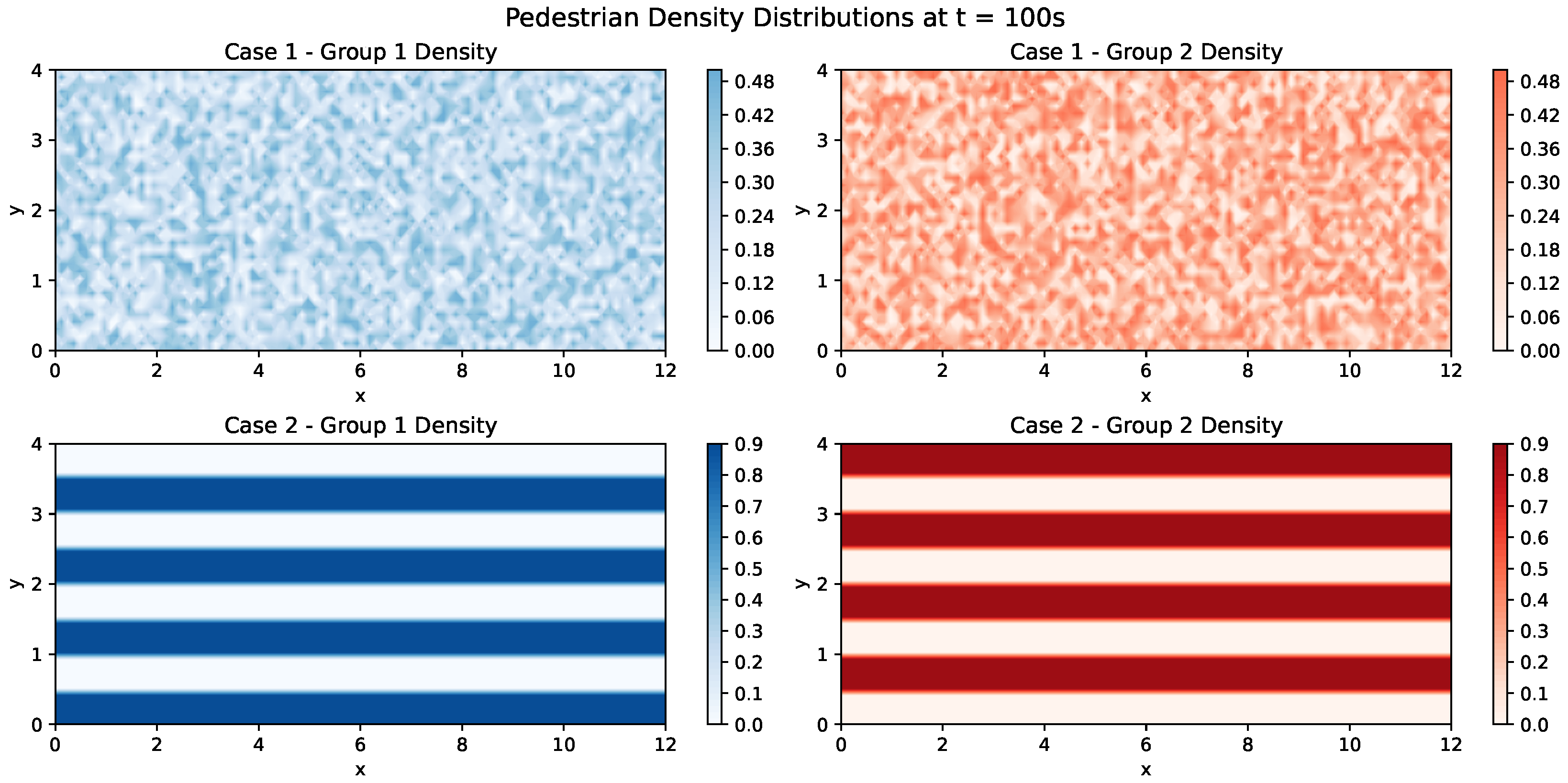
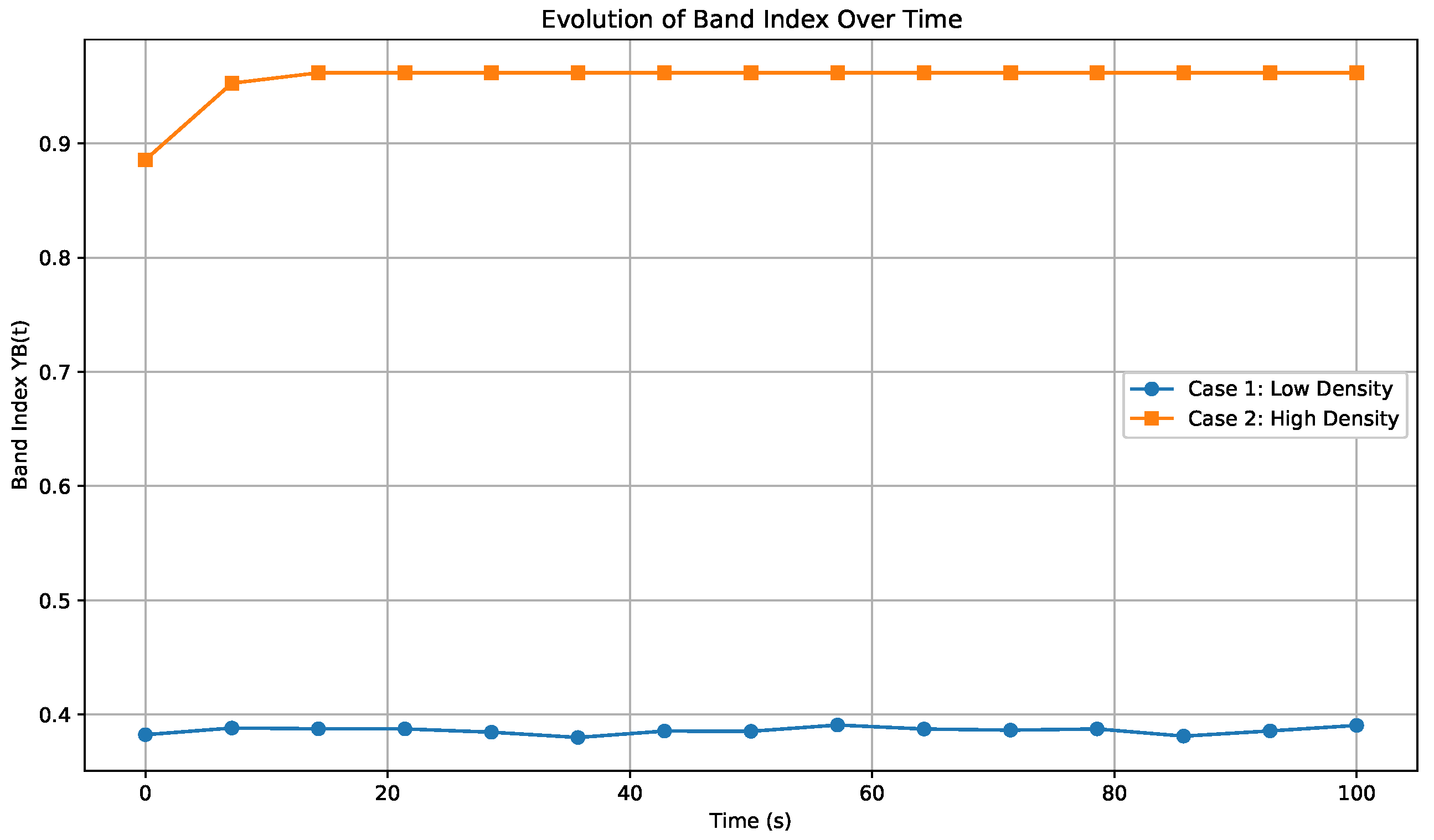
As illustrated in Figure 4 and Figure 5, in Case 1, where the crowd density is low, the band index, which was initially 0.38, remains relatively stable over time. Pedestrians distribute randomly across the domain, and no segregation occurs. In contrast, in Case 2, which involves a denser crowd, the band index shows a significant increase, as depicted in Figure 4 and Figure 5.
In addition, the emergence of spatial segregation is apparent, with the two groups of pedestrians forming in alternating lines and files. It is worth pointing out that unlike most previous studies on the subject, this emergent behavior has not been achieved by introducing a repulsion force between pedestrians of different populations [4,18].
Finally, as shown in Figure 4, the counterflow of pedestrian social groups exhibits a self-organizing behavior, leading to the formation of lanes with uniform walking directions. This pattern significantly enhances movement efficiency and reduces friction between opposing groups [4,18].

5. Critical Analysis and Perspectives

In this paper, a kinetic model has been proposed to simulate counterflows within pedestrian social groups in a corridor, focusing on interactions both within the same group and between different groups moving in opposite directions. An advanced numerical method, based on the Monte Carlo particle method, has been developed. Numerical simulation scenarios have been employed to capture the emergent behavior of lane formation, a crucial feature of bidirectional pedestrian flow. The model’s ability to replicate empirical patterns of collective motion highlights its potential for practical applications in crowd management and safety.
The main objective of the simulations has been to demonstrate the spontaneous segregation of pedestrians into lanes with uniform walking directions, as highlighted by the results in Figure 4 and Figure 5. Nevertheless, there are some limitations in the model proposed in the present paper. Indeed, this model considers the variable u as a deterministic parameter representing the movement preference of each social group. Although it captures some degree of heterogeneity among pedestrian social groups, it remains limited in representing the full spectrum of behavioral diversity. In future work, we aim to overcome this limitation by modeling u as an activity variable with its own dynamics, as discussed in [3]. This approach can account for the propagation of stress [11], emotional contagion, and learning levels by incorporating a follower–leader structure [12], thereby enabling the modeling of multiple interacting social groups.
As already mentioned, the model captures only a limited degree of heterogeneity among pedestrian social groups. Addressing the challenges in social group dynamics simulation requires integrating advanced data-driven techniques with physics-based frameworks to better represent the complexity and variability of real-world pedestrian behavior [7,50]. Therefore, future studies will focus on enhancing the model to more accurately simulate the impact of pedestrian social group behavior in counterflow situations [28,29,30].
It is worth stressing that the mathematical framework and the related specific model proposed in this paper are at equilibrium; namely the action of an external force field is not modeled. In order to model real out-of-equilibrium events, during which the pedestrian dynamics is modified not only by the internal interactions among the pedestrians but also by the action of an external event (e.g., evacuation), generalizations of the framework proposed in the paper need to be taken into account. Recently the thermostatted kinetic theory for active particles has been proposed and employed for the modeling of out-of-equilibrium complex living systems, such as pedestrians dynamics [51,52] and biological systems [53]. The mathematical framework of the thermostatted kinetic theory includes a damping term which models and controls the action of an external force field and allows it to reach nonequilibrium stationary states. Moreover the simulation of the damping term, called the Gaussian thermostat, requires further developments of the Monte Carlo simulation method. This is an important research perspective, and the results will be presented in due course.

Author Contributions

Conceptualization, N.B. and A.H.; methodology, N.B.; software, N.B.; validation, N.B.; writing—original draft preparation, N.B., C.B. and A.H.; writing—review and editing, N.B., C.B. and A.H.; supervision, A.H. All authors have read and agreed to the published version of the manuscript.

Funding

This research received no external funding.

Data Availability Statement

Data are contained within the article.

Acknowledgments

The authors sincerely thank the reviewers for their insightful comments and constructive suggestions, which have greatly improved the quality of this work.

Conflicts of Interest

The authors declare no conflicts of interest.

References

  1. Feliciani, C.; Jia, X.; Murakami, H.; Ohtsuka, K.; Vizzari, G.; Nishinari, K. Social groups in pedestrian crowds as physical and cognitive entities: Extent of modeling and motion prediction. Transp. Res. Part A Policy Pract. 2023, 176, 103820. [Google Scholar] [CrossRef]
  2. Nicolas, A.; Hassan, F.H. Social groups in pedestrian crowds: Review of their influence on the dynamics and their modelling. Transp. A Transp. Sci. 2023, 19, 1970651. [Google Scholar] [CrossRef]
  3. Bellomo, N.; Gibelli, L.; Quaini, A.; Reali, A. Towards a mathematical theory of behavioral human crowds. Math. Models Methods Appl. Sci. 2022, 32, 321–358. [Google Scholar] [CrossRef]
  4. Bellomo, N.; Liao, J.; Quaini, A.; Russo, L.; Siettos, C. Human behavioral crowds: Review, critical analysis, and research perspectives. Math. Models Methods Appl. Sci. 2023, 33, 1611–1659. [Google Scholar] [CrossRef]
  5. Knopoff, D.A.; Liao, J.; Ma, Q.; Yang, X. Individual-based crowd dynamics with social interaction. Math. Models Methods Appl. Sci. 2025, 35, 1637–1660. [Google Scholar] [CrossRef]
  6. Gibelli, L.; Knopoff, D.A.; Liao, J.; Yan, W. Macroscopic modeling of social crowds. Math. Models Methods Appl. Sci. 2024, 34, 1135–1151. [Google Scholar] [CrossRef]
  7. Bellomo, N.; Dolfin, M.; Liao, J. Life and self-organization on the way to artificial intelligence for collective dynamics. Phys. Life Rev. 2024, 51, 1–8. [Google Scholar] [CrossRef]
  8. Bakhdil, N.; El Mousaoui, A.; Hakim, A. A kinetic BGK model for pedestrian dynamics accounting for anxiety conditions. Symmetry 2025, 17, 19. [Google Scholar] [CrossRef]
  9. Bellomo, N.; Burini, D.; Dosi, G.; Gibelli, L.; Knopoff, D.; Outada, N.; Terna, P.; Virgillito, M.E. What is life? A perspective of the mathematical kinetic theory of active particles. Math. Models Methods Appl. Sci. 2021, 31, 1821–1866. [Google Scholar] [CrossRef]
  10. Elaiw, A.; Al-Turki, Y. Particle methods simulations by kinetic theory models of human crowds accounting for stress conditions. Symmetry 2020, 12, 14. [Google Scholar] [CrossRef]
  11. Bellomo, N.; Gibelli, L.; Outada, N. On the interplay between behavioral dynamics and social interactions in human crowds. Kinet. Relat. Models 2019, 12, 397–409. [Google Scholar] [CrossRef]
  12. Liao, J.; Ren, Y.; Yan, W. Kinetic modeling of a leader–follower system in crowd evacuation with collective learning. Math. Models Methods Appl. Sci. 2023, 33, 1099–1117. [Google Scholar] [CrossRef]
  13. Eftimie, R.; Gibelli, L. A kinetic theory approach for modelling tumour and macrophages heterogeneity and plasticity during cancer progression. Math. Models Methods Appl. Sci. 2020, 30, 659–683. [Google Scholar] [CrossRef]
  14. Bellomo, N.; Bingham, R.; Chaplain, M.A.J.; Dosi, G.; Forni, G.; Knopoff, D.A.; Lowengrub, J.; Twarock, R.; Virgillito, M.E. A multiscale model of virus pandemic: Heterogeneous interactive entities in a globally connected world. Math. Models Methods Appl. Sci. 2020, 30, 1591–1651. [Google Scholar] [CrossRef]
  15. Zagour, M. Modeling and numerical simulations of multilane vehicular traffic by active particles methods. Math. Models Methods Appl. Sci. 2023, 33, 1119–1146. [Google Scholar] [CrossRef]
  16. Bellomo, N.; Bellouquid, A. On the modeling of crowd dynamics: Looking at the beautiful shapes of swarms. Netw. Heterog. Media 2011, 6, 383–399. [Google Scholar] [CrossRef]
  17. Bellomo, N.; Bellouquid, A.; Knopoff, D. From the microscale to collective crowd dynamics. Multiscale Model. Simul. 2013, 11, 943–963. [Google Scholar] [CrossRef]
  18. Bellomo, N.; Gibelli, L. Toward a mathematical theory of behavioral-social dynamics for pedestrian crowds. Math. Models Methods Appl. Sci. 2015, 25, 2417–2437. [Google Scholar] [CrossRef]
  19. Elmoussaoui, A.; Argoul, P.; El Rhabi, M.; Hakim, A. Discrete kinetic theory for 2D modeling of a moving crowd: Application to the evacuation of a non-connected bounded domain. Comput. Math. Appl. 2018, 75, 1159–1180. [Google Scholar] [CrossRef]
  20. Kim, D.; Quaini, A. A kinetic theory approach to model pedestrian dynamics in bounded domains with obstacles. Kinet. Relat. Models 2019, 12, 1273–1296. [Google Scholar] [CrossRef]
  21. Liao, J.; Zhou, L. A kinetic modeling of crowd evacuation with several groups in complex venues. Math. Models Methods Appl. Sci. 2022, 32, 1785–1805. [Google Scholar] [CrossRef]
  22. Kim, D.; Labate, D.; Mily, K.; Quaini, A. Data-driven learning to enhance a kinetic model of distressed crowd dynamics. Math. Models Methods Appl. Sci. 2025, 35, 1609–1636. [Google Scholar] [CrossRef]
  23. Bellomo, N.; Gibelli, L. Behavioral crowds: Modeling and Monte Carlo simulations toward validation. Comput. Fluids 2016, 141, 13–21. [Google Scholar] [CrossRef]
  24. Agnelli, J.P.; Armas, C.; Knopoff, D.A. Spatial kinetic modeling of crowd evacuation: Coupling social behavior and infectious disease contagion. Symmetry 2025, 17, 123. [Google Scholar] [CrossRef]
  25. Kim, D.; O’Connell, K.; Ott, W.; Quaini, A. A kinetic theory approach for 2D crowd dynamics with emotional contagion. Math. Models Methods Appl. Sci. 2021, 31, 1137–1162. [Google Scholar] [CrossRef]
  26. Kim, D.; Quaini, A. Coupling kinetic theory approaches for pedestrian dynamics and disease contagion in a confined environment. Math. Models Methods Appl. Sci. 2020, 30, 1893–1915. [Google Scholar] [CrossRef]
  27. Bode, N.W.; Holl, S.; Mehner, W.; Seyfried, A. Disentangling the impact of social groups on response times and movement dynamics in evacuations. PLoS ONE 2015, 10, e0121227. [Google Scholar] [CrossRef]
  28. Moussaïd, M.; Perozo, N.; Garnier, S.; Helbing, D.; Theraulaz, G. The walking behaviour of pedestrian social groups and its impact on crowd dynamics. PLoS ONE 2010, 5, e10047. [Google Scholar] [CrossRef]
  29. Haghani, M.; Yazdani, M. How behavioural changes in social groups affect evacuation efficiency of crowds. Saf. Sci. 2025, 181, 106679. [Google Scholar] [CrossRef]
  30. Fu, L.; Shi, Q.; Qin, H.; Zhang, Y.; Shi, Y. Analysis of movement behavior of pedestrian social groups through a bottleneck. Phys. A Stat. Mech. Appl. 2022, 608, 128257. [Google Scholar] [CrossRef]
  31. He, Y.; Shi, Q.; Fu, L.; Chen, Q.; Shen, C.; Zhang, Y.; Shi, Y.; Lo, J.T.Y. Application of the multi-grid modelling method to pedestrian social group dynamics through a bottleneck. Simul. Model. Pract. Theory 2025, 139, 103049. [Google Scholar] [CrossRef]
  32. Lu, L.; Chan, C.-Y.; Wang, J.; Wang, W. A study of pedestrian group behaviors in crowd evacuation based on an extended floor field cellular automaton model. Transp. Res. Part C Emerg. Technol. 2017, 81, 317–329. [Google Scholar] [CrossRef]
  33. Li, C.-Y.; Yang, R.-Y.; Xu, G.-M. Impacts of group behavior on boarding process at the platform of high-speed railway station. Phys. A Stat. Mech. Appl. 2019, 535, 122247. [Google Scholar] [CrossRef]
  34. Crociani, L.; Zeng, Y.; Vizzari, G.; Bandini, S. Shape matters: Modelling, calibrating and validating pedestrian movement considering groups. Simul. Model. Pract. Theory 2018, 87, 73–91. [Google Scholar] [CrossRef]
  35. Crociani, L.; Gorrini, A.; Vizzari, G. Pedestrian dynamics in presence of groups: An agent-based model applied to a real world case study. In Proceedings of the 13th International Conference on Autonomous Agents and Multiagent Systems Workshops, Paris, France, 5–9 May 2014. [Google Scholar]
  36. Turgut, Y.; Bozdag, C.E. Modeling pedestrian group behavior in crowd evacuations. Fire Mater. 2022, 46, 420–442. [Google Scholar] [CrossRef]
  37. Ivo, D.; Cavalcante-Neto, J.; Vidal, C. A model for flexible representation of social groups in crowd simulation. Comput. Graph. 2021, 101, 7–22. [Google Scholar] [CrossRef]
  38. Prédhumeau, M.; Dugdale, J.; Spalanzani, A. Modeling and simulating pedestrian social group behavior with heterogeneous social relationships. In Proceedings of the 2020 Spring Simulation Conference (SpringSim), Fairfax, VA, USA, 18–21 May 2020; pp. 1–12. [Google Scholar]
  39. Rozan, E.; Frank, G.; Cornes, F.; Sticco, I.; Dorso, C. Microscopic dynamics of escaping groups through an exit and a corridor. Phys. A Stat. Mech. Appl. 2022, 597, 127271. [Google Scholar] [CrossRef]
  40. Xie, W.; Lee, E.W.M.; Li, T.; Shi, M.; Cao, R.F.; Zhang, Y.C. A study of group effects in pedestrian crowd evacuation: Experiments, modelling and simulation. Saf. Sci. 2021, 133, 105029. [Google Scholar] [CrossRef]
  41. Bakhdil, N.; El Mousaoui, A.; Hakim, A. A kinetic theory approach to model pedestrian social groups behavior in bounded domain. Kinet. Relat. Models 2024, 17, 88–106. [Google Scholar] [CrossRef]
  42. Ye, R.; Fang, Z.; Lian, L.; Wang, Q.; Zeng, G.; Cao, S.; Zhang, J.; Song, W. Traffic dynamics of uni- and bidirectional pedestrian flows including dyad social groups in a ring-shaped corridor. J. Stat. Mech. Theory Exp. 2021, 2021, 023406. [Google Scholar] [CrossRef]
  43. Yamori, Y. Going with the flow: Micro-macro dynamics in the macrobehavioral patterns of pedestrian crowds. Psychol. Rev. 1998, 105, 530–557. [Google Scholar] [CrossRef]
  44. Buchmüller, S.; Weidmann, U. Parameters of Pedestrians, Pedestrian Traffic and Walking Facilities; IVT Report Nr. 132; Institute for Transport Planning and Systems (IVT), Swiss Federal Institute of Technology Zurich (ETHZ): Zurich, Switzerland, 2006. [Google Scholar]
  45. Pareschi, L.; Toscani, G. Interacting Multiagent Systems: Kinetic Equations and Monte Carlo Methods; Oxford University Press: Oxford, UK, 2014. [Google Scholar]
  46. Rjasanow, S.; Wagner, W. Stochastic Numerics for the Boltzmann Equation; Springer: Berlin/Heidelberg, Germany, 2005. [Google Scholar]
  47. Fang, J.; El-Tawil, S.; Aguirre, B. Leader–follower model for agent-based simulation of social collective behavior during egress. Saf. Sci. 2016, 83, 40–47. [Google Scholar] [CrossRef]
  48. Forschungszentrum Jülich. Pedestrian Dynamics Data Archive. Available online: https://ped.fz-juelich.de/database/doku.php?id=extdb (accessed on 29 April 2025).
  49. Nowak, S.; Schadschneider, A. Quantitative analysis of pedestrian counterflow in a cellular automaton model. Phys. Rev. E 2012, 85, 066128. [Google Scholar] [CrossRef] [PubMed]
  50. Quarteroni, A.; Gervasio, P.; Regazzoni, F. Combining physics-based and data-driven models: Advancing the frontiers of research with scientific machine learning. Math. Models Methods Appl. Sci. 2025, 35, 905–1071. [Google Scholar] [CrossRef]
  51. Bianca, C.; Mogno, C. Qualitative analysis of a discrete thermostatted kinetic framework modeling complex adaptive systems. Commun. Nonlinear Sci. Numer. Simulat. 2018, 54, 221–232. [Google Scholar] [CrossRef]
  52. Bianca, C. The role of the table of games in the discrete thermostatted kinetic theory. Mathematics 2024, 12, 2356. [Google Scholar] [CrossRef]
  53. Bianca, C. A decade of thermostatted kinetic theory models for complex active matter living systems. Phys. Life Rev. 2024, 50, 72–97. [Google Scholar] [CrossRef]
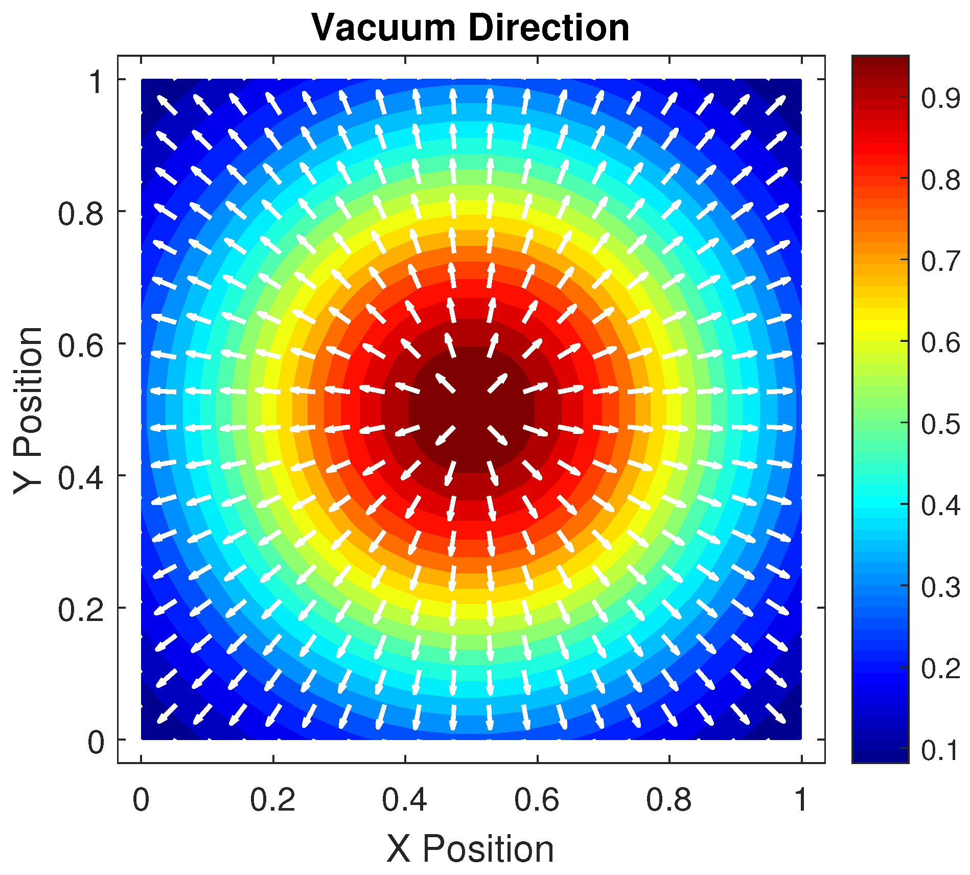
Figure 2. v ( v a c u u m ) direction.
Mathematics 13 02788 g002
Figure 3. Perceived density vs. density gradient.
Mathematics 13 02788 g003
Figure 4. Bidirectional flow of pedestrian social groups for β = 0.75 . Above panel: Density contour plots of case 1 at time t = 100 s . Below panel: Density contour plots of case 2 at time t = 100 s .
Mathematics 13 02788 g004
Figure 5. Temporal evolution of Yamori’s band index Y B a n d .
Mathematics 13 02788 g005
Table 1. The walker’s decision process during interactions between walkers of the same social group.
ConditionTransitionProbability
θ θ θ = θ ( p ) [ ρ i , ξ i ] 1
Interactions between v v = v a i p a i
walkers of the same v | | ξ i | |
i-th social group v v = v 1 p a i
v v = v d i p d i
v > | | ξ i | |
v v = v 1 p d i
Table 2. The walker’s decision process during interactions between walkers of the i-th social group with other social groups.
ConditionTransitionProbability
θ θ θ = θ ( p ) [ ρ , ξ ] 1
v v = v a c i r a i
Interactions between v | | ξ | |
walkers of i-th social group v v = v 1 r a i
with other social groups
v v = v d e i r d i
v > | | ξ | |
v v = v 1 r d i
Disclaimer/Publisher’s Note: The statements, opinions and data contained in all publications are solely those of the individual author(s) and contributor(s) and not of MDPI and/or the editor(s). MDPI and/or the editor(s) disclaim responsibility for any injury to people or property resulting from any ideas, methods, instructions or products referred to in the content.