Deep Learning for Bifurcation Detection: Extending Early Warning Signals to Dynamical Systems with Coloured Noise

Abstract

Deep learning models have demonstrated remarkable success in recognising tipping points and providing early warning signals. However, there has been limited exploration of their application to dynamical systems governed by coloured noise, which characterizes many real-world systems. In this study, we show that it is possible to leverage the normal forms of three primary types of bifurcations (fold, transcritical, and Hopf) to construct a training set that enables deep learning architectures to perform effectively. Furthermore, we showed that this approach could accommodate coloured noise by replacing white noise with red noise during the training process. To evaluate the classifier trained on red noise compared to one trained on white noise, we tested their performance on mathematical models using Receiver Operating Characteristic (ROC) curves and Area Under the Curve (AUC) scores. Our findings reveal that the deep learning architecture can be effectively trained on coloured noise inputs, as evidenced by high validation accuracy and minimal sensitivity to redness (ranging from 0.83 to 0.85). However, classifiers trained on white noise also demonstrate impressive performance in identifying tipping points in coloured time series. This is further supported by high AUC scores (ranging from 0.9 to 1) for both classifiers across different coloured stochastic time series.

1. Introduction

Dynamical systems are employed to describe various phenomena across disciplines, from studying the climate system [1,2,3] to epidemiological studies [4,5,6], rumour propagation mechanisms [7], and coupled behaviour–disease dynamics [8]. While dynamical systems exhibit numerous intriguing aspects, one particularly captivating focus in recent years has been the possibility of bifurcation and tipping points [8,9,10,11]. In natural systems, a local bifurcation can occur as external conditions gradually change, bringing the system near an equilibrium state and potentially triggering a qualitative shift in behaviour when a tipping point is reached [12,13].

Bifurcation theory is a rich branch of mathematics that delves into the theoretical properties of dynamical systems experiencing different types of bifurcations [14]. One of its most significant theories, the Centre Manifold Theorem, along with the Normal Form Theorem, simplifies nonlinear dynamical systems by transforming them into their simplest equivalent form, termed the “normal form”. Through coordinate transformations, it eliminates unnecessary nonlinear terms while preserving the system’s essential behaviour, making it easier to examine features like bifurcations [15,16,17].

While these theorems are generally valid, this paper specifically focuses on three types of local bifurcations, as they represent distinct behaviours in dynamical systems: the abrupt jump from one equilibrium state to another (fold bifurcation) [18], smoothly shifting stability (transcritical bifurcation) [19], and the transition to oscillatory behaviour (Hopf bifurcation) [20]. For these bifurcation types, the dominant eigenvalue of the derivative matrix crosses the imaginary axis at the bifurcation point. Leading up to the bifurcation, the system can exhibit critical slowing down, corresponding to prolonged recovery from perturbations and reduced resilience to disturbances, as measured by increased auto-correlation and variance [21]. Numerous generic indicators of local bifurcations have been proposed based on these consequences [22,23,24,25]. For instance, the variance and lag-1 auto-correlation of a time series prior to bifurcation shows trends that can serve as early warning signals (EWSs) [26]. While such indicators have been instrumental in identifying and predicting tipping points and abrupt shifts, they also possess limitations [27], such as an inability to specify the type of impending bifurcation. With recent advances in artificial intelligence (AI) and the development of deep learning (DL) models, it was anticipated that these models could eventually provide EWSs with greater accuracy and fewer weaknesses than generic indicators.

The first study applying AI to the detection of tipping points in dynamical systems is by Bury et al. [28], who showed that convolutional and recurrent neural networks could identify EWS in time series drawn from a random library of differential equations. Their approach demonstrated that DL architectures could outperform traditional statistical indicators. Deb et al. [29] introduced EWSNet, a hybrid Convolutional Neural Network–Long Short-Term Memory (CNN-LSTM) network trained on simulated time series from ecological, biological, and climate models. EWSNet showed high accuracy in classifying catastrophic and non-catastrophic transitions and proved robust to noise, short time series, and irregular sampling. These previous works were extended in a follow-up study by Bury et al. [30] to discrete-time systems, further validating the generalizability of DL models to diverse bifurcation scenarios. Dylewsky et al. [31] demonstrated that universal EWSs could be extracted from DL models trained on climate system simulations, supporting the broader applicability of these methods. Dylewsky et al. [25] advanced this work by embedding bifurcations in high-dimensional systems, showing that DL models remain effective even when the underlying signals are distributed across many variables. Most recently, Huang et al. [32] addressed the challenge of rate-induced tipping (R-tipping), where classical indicators like critical slowing down fail. Their interpretable DL framework predicted transition probabilities in noisy, time-varying systems and extracted higher-order fingerprints of instability. In parallel, Dylewsky et al. [33] tackled spatially patterned phase transitions using neural architectures tailored for spatiotemporal systems. Together, these studies illustrate a growing body of work that supports the use of deep learning, with CNN–LSTM architectures being one of the main and most effective models for robust and generalizable detection of critical transitions in noisy, nonlinear dynamical systems.

In contrast to previous approaches that generate extensive libraries of stochastic differential equations and discard those that do not exhibit bifurcations [30], we propose a theoretically grounded method by constructing the training dataset directly from the normal forms of canonical bifurcations. This significantly reduces computational overhead while ensuring that the training data captures the essential dynamical features associated with each bifurcation type. The first objective of this study is to demonstrate that such a targeted construction is not only feasible but also more efficient than relying on random dynamical systems. Furthermore, we extend the DL-based early warning framework of [28] to accommodate coloured noise, a feature often overlooked despite its prevalence in empirical systems. Many ecological and climate systems that undergo critical transitions are influenced by auto-correlated, coloured noise [34,35], prompting recent interest in its ecological impacts [36,37,38,39,40,41,42,43,44,45]. By generating training data with varying levels of redness, we evaluate the robustness of our CNN-LSTM classifier under both white and coloured noise, enhancing the applicability of EWS frameworks to real-world, noisy, nonlinear systems.

2. Methods

2.1. Model Selection Rationale

To construct the deep learning model, we employed a hybrid architecture combining a CNN with an LSTM network [46,47,48]. Theoretically, the CNN layers serve to extract local patterns and short-term features from the time series by applying convolutional filters, while the LSTM layers are designed to capture long-range temporal dependencies through their recurrent structure. This layered combination is particularly well-suited for our task, as it enables both local pattern detection and memory retention—key components in identifying EWSs indicative of critical transitions.

The CNN-LSTM architecture has been widely adopted in the broader literature on time series forecasting and classification. For instance, ref. [49] demonstrated that CNN–LSTM achieved the highest forecasting accuracy across multiple benchmarks, outperforming standalone models such as Multilayer Perceptron (MLP), CNN, recurrent neural network (RNN), and LSTM. Similarly, ref. [50] evaluated CNN, LSTM, and CNN–LSTM on ice-jam event classification and reported superior F1-scores for the CNN–LSTM model. In the context of missing data imputation, ref. [51] showed that CNN–LSTM achieved better predictive accuracy than either CNN or LSTM alone when forecasting electricity consumption. More specifically, architectures similar to ours have been increasingly applied to problems involving bifurcation detection and phase transitions in dynamical systems. Recent studies such as [25,28,30,31,33] have demonstrated that CNN–LSTM models are effective at detecting EWSs in stochastic systems and outperforming simpler baselines.

To justify our choice of DL model, we conducted an ablation study comparing the performance of LSTM-only and CNN-LSTM architectures. Both models were trained and tested on time series generated with white noise, using identical hyperparameter settings to ensure a fair comparison. To ensure a fair evaluation, we tested both the LSTM-only and CNN-LSTM models on time series generated using the same process as the training dataset. The results, presented in

Table 1. Comparison of overall performance metrics between CNN-LSTM and LSTM-only models.

Metric	CNN-LSTM	LSTM-Only
Accuracy Score	0.823	0.773
F1-Score	0.822	0.769
Precision	0.834	0.778
Recall	0.823	0.773

, show that while the LSTM-only model achieves reasonably strong performance, the CNN-LSTM consistently outperforms it in terms of accuracy, precision, recall, and F1-score. This supports our choice of architecture and aligns with findings from previous work, such as [28], which also highlighted the superiority of CNN-LSTM over LSTM-only models in similar dynamical settings. Both the CNN–LSTM and LSTM-only models were trained on the same dataset from normal forms with white noise, using identical settings and pre-processing. The LSTM-only model shares the recurrent layers of the CNN–LSTM but omits the convolutional block. Hyperparameters were guided by [28] and further tuned through experiments to optimize performance. Full details are provided in the Section 5.

2.2. Constructing Training Data Set

The training dataset was created by stochastically simulating the normal forms of different types of bifurcations (fold, transcritical, Hopf). In each case, we began at the system’s equilibrium point, far from the bifurcation point, and then gradually and linearly moved the system closer to the bifurcation point. These time series were classified into three categories, with an additional “null” category created by simulating white/coloured noise alone. Using this dataset, we trained the CNN-LSTM model to classify time series into the four defined categories.

This method can be generalised to coloured noise by replacing white noise with red noise in the additive stochastic process of simulations. We generated red noise using the Auto-Regressive model of order 1 (AR(1)) method.

$$X_{t+1}=(\mathrm{redness}·X_t)+\sqrt{1-{\mathrm{redness}}^2}·{ϵ}_t$$

(1)

With $X_0\sim N(0, 1)$. This recursive equation is controlled by a redness parameter between 0 and 1. If the redness equals zero, the process generates white noise, and the larger the redness, the more coloured and auto-correlated the process becomes. Additionally, ${ϵ}_t$ is a stochastic variable drawn from a Gaussian distribution $N(0, 1)$.

We simulated 20,000 time series in total, using 90% of them for the training process. The remaining 10% was used to test the performance of the DL model.

Table 2. Model performance metrics across redness levels.

Redness	Validation Accuracy	Accuracy Score	F1-Score	Precision	Recall
0.0	0.852	0.826	0.825	0.829	0.827
0.1	0.857	0.831	0.829	0.832	0.832
0.2	0.857	0.833	0.834	0.836	0.837
0.3	0.853	0.834	0.836	0.8476	0.8355
0.4	0.831	0.841	0.838	0.847	0.84
0.5	0.832	0.864	0.864	0.866	0.864

summarises the model performance metrics across redness levels.

The redness values range from 0.0 to 0.5, where higher values indicate stronger auto-correlation in the input noise. The validation accuracy and other performance metrics remain relatively stable across this range, with a peak of 85% observed at redness values of 0.0, 0.1, 0.2, and 0.3. A slight drop to 83% is seen at the extreme values (0.4 and 0.5), suggesting minimal sensitivity of the model’s performance to changes in noise persistence. This demonstrates that the DL architecture can be trained effectively on coloured noise inputs as well. The details of the confusion matrix and classification metrics are provided in the Section 5.

In addition, we include further discussion on the robustness of the training process, the minimum data requirements, and full technical details on simulating the training dataset.

3. Results

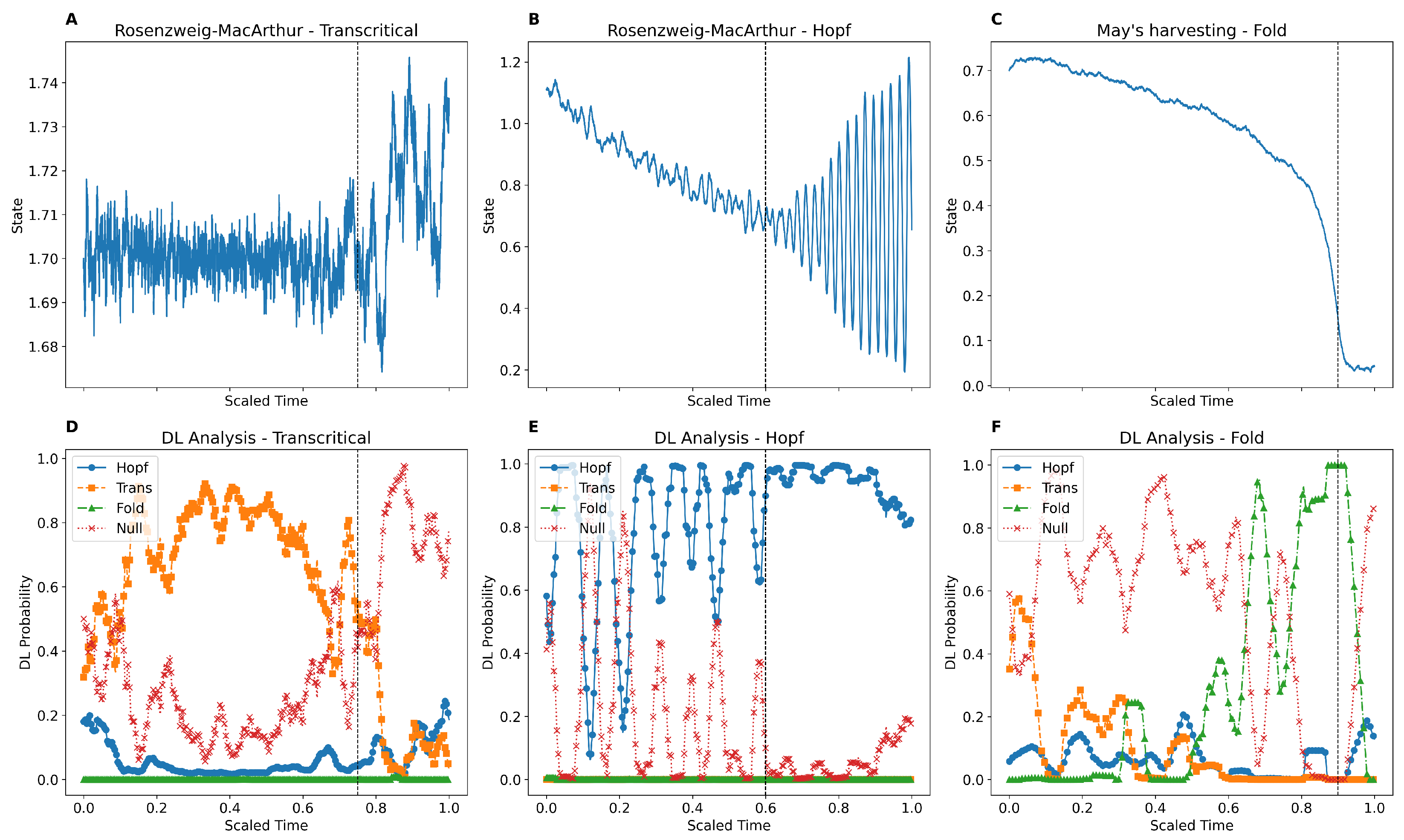
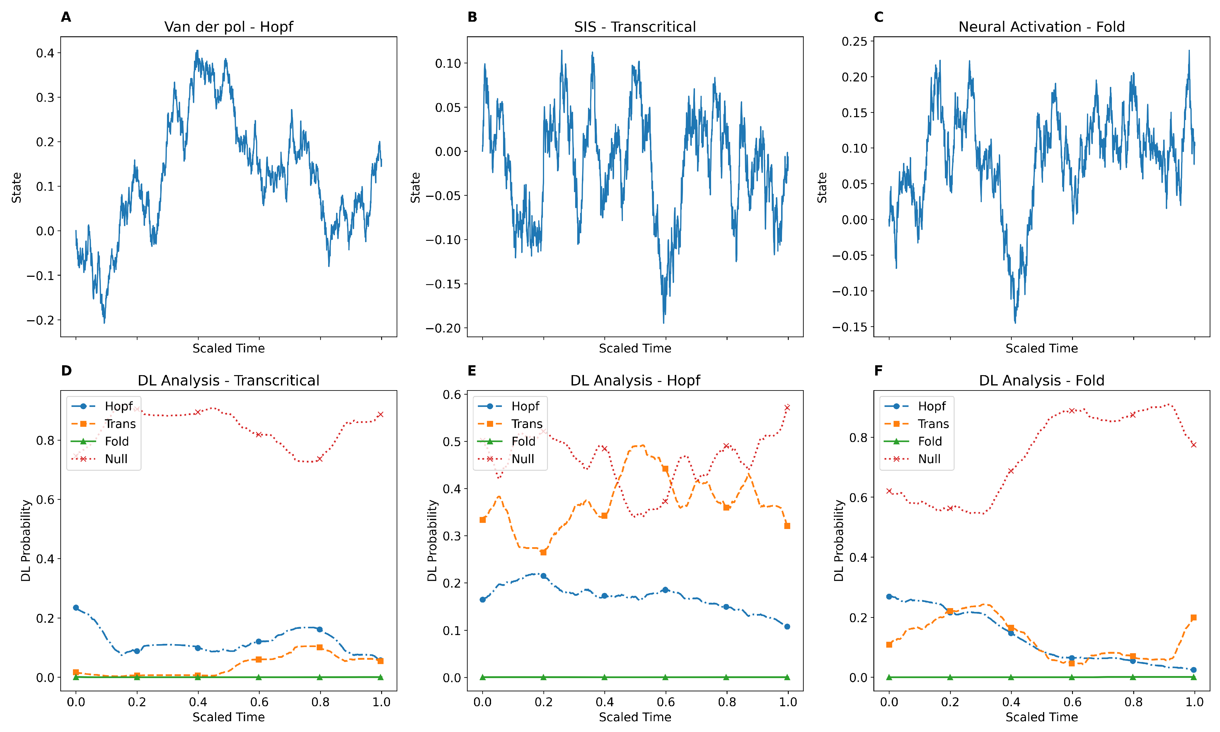
We have demonstrated that the DL model can provide EWS for bifurcations in mathematical models. For this purpose, we utilised six well-known mathematical models: neural activation and May’s harvesting model for fold bifurcation, the Rosenzweig–MacArthur and SIS models for transcritical bifurcation, and the Rosenzweig–MacArthur and Van der Pol models for Hopf bifurcation. We simulated these mathematical models with an additive stochastic term, starting from the equilibrium point and linearly varying the bifurcation parameter toward the bifurcation point throughout the simulation. Since the tipping point can occur earlier than the theoretical prediction, we employed the binary segmentation algorithm to locate the tipping point. The DL model assigns four probabilities (fold, transcritical, Hopf, and null) to each point in the simulated time series. The null category in our study represents stochastic time series that either do not include a tipping point or are relatively distant from it. Assigning a relatively high probability to the correct type of bifurcation before the actual location of the tipping point is considered a signal in this study. Figure 1 and Figure 2 depict the results of the DL analysis of the introduced mathematical models. The estimated location of the tipping point is indicated on the plots with a dashed line. As shown, the DL model is not only capable of providing EWS but also accurately identifies the correct type of bifurcation. Furthermore, at the beginning of the simulated time series, where the tipping point is relatively distant, the DL model assigns the highest probability to null. As the series approaches the tipping point, the model transitions to selecting the correct type of bifurcation and then returns to assigning null after the tipping point has passed. This behaviour is consistent with the observations from the analysis of all six mathematical models. The mathematical descriptions, full details of the simulations, and null analyses are provided in the Section 5.

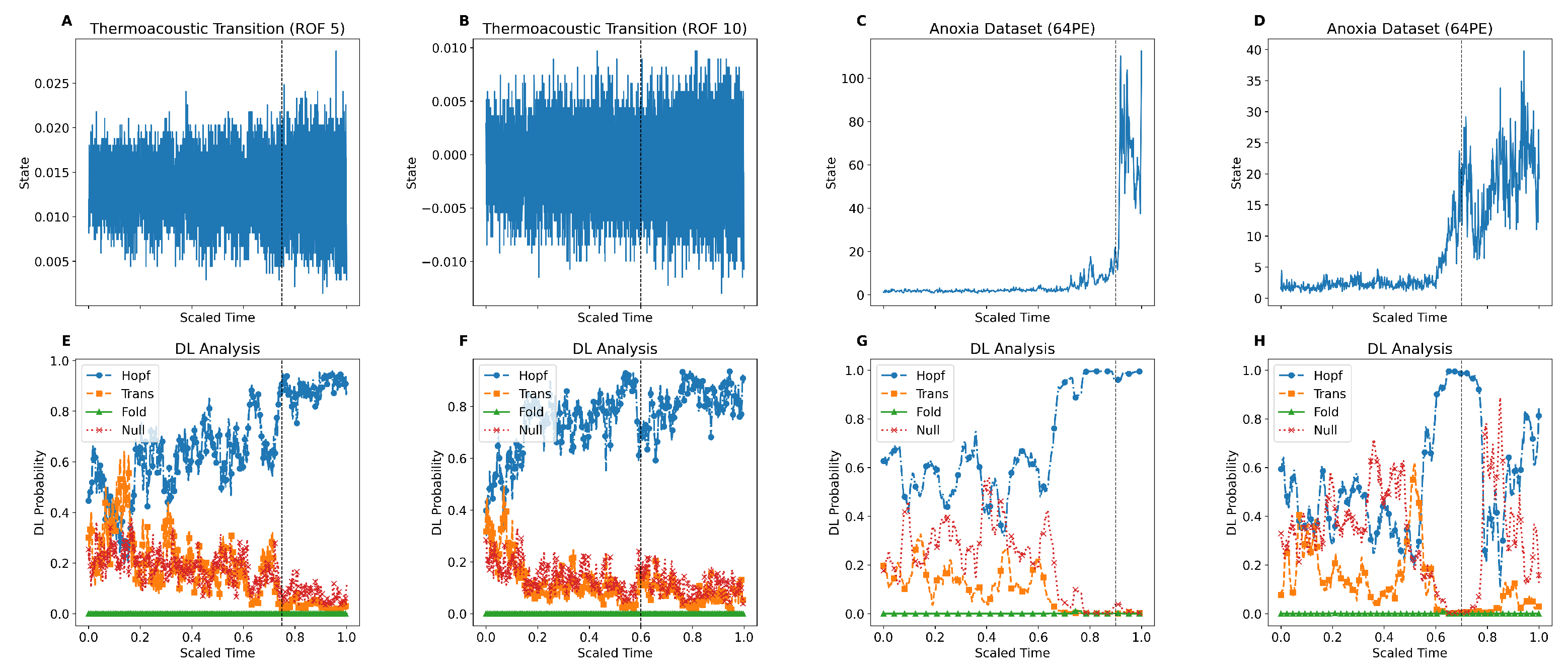
In addition, we have demonstrated that the DL model exhibits robust performance in providing EWS on empirical data containing tipping points. We analysed two sets of empirical data: one representing the transition to thermoacoustic instability in a horizontal Rijke tube, a prototypical thermoacoustic system, and the other capturing episodes of anoxia in the Eastern Mediterranean from sedimentary archives. To ensure proper resolution and quality for the analysis, we expanded the size of the time series for these datasets using the Linear Interpolation method. Figure 3 illustrates the results of the DL analysis on four examples of these time series (two from each dataset). The estimated location of the tipping point is indicated with a dashed line on each subplot. As shown, the DL model successfully provides EWS on these time series before the actual tipping point, transitioning from assigning null to identifying one of the types of bifurcation. Notably, for the anoxia data, the DL classifier predicts a Hopf transition, whereas the empirical data suggest a transition more akin to a fold-type bifurcation. Additional analysis on empirical data is provided in the Section 5.

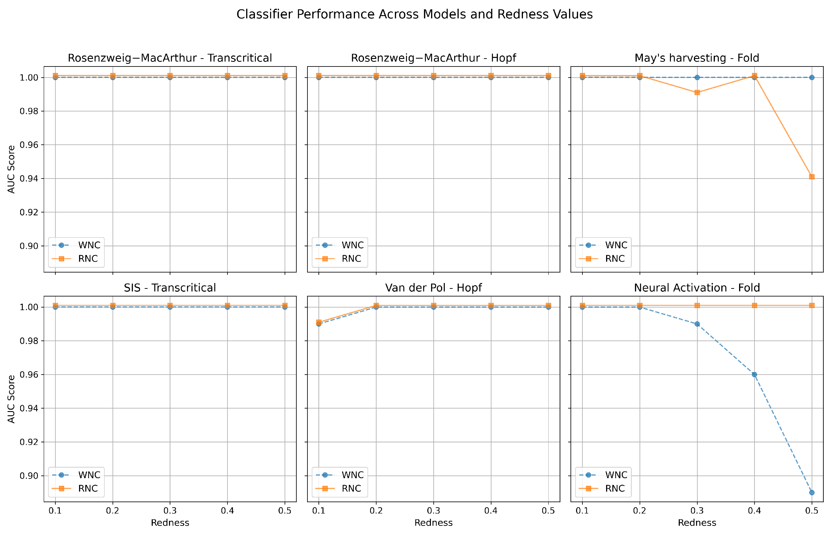
Moreover, the DL model demonstrates consistent success with stochastic time series that include coloured noise. To illustrate this, we repeated the same training process using the same DL architecture (CNN-LSTM), but this time incorporated red noise (with specific redness values) as an additive stochastic term while simulating the deterministic normal forms of different types of bifurcation. As a result, we generated five additional DL classifiers, each trained on normal forms combined with red noise (redness values of 0.1, 0.2, 0.3, 0.4, and 0.5). A larger redness value in red noise signifies greater dominance of low-frequency components, stronger persistence, and smoother, long-term variability in the time series. Note that the baseline DL model used in previous sections is based on white noise and can be considered a special case of this process with a redness value of 0. To quantify and compare the performance of the red noise classifier against the white noise classifier, we simulated stochastic time series for the six mathematical models using different redness values (ranging from 0 to 0.5). Each mathematical model was simulated 50 times, and the ROC curves for all classifiers were plotted. By calculating the AUC score for each classifier across mathematical models and redness values, we could compare their performance. The objective was to demonstrate that the DL model trained on white noise can maintain strong performance in detecting bifurcations on time series that include red noise. This expectation is confirmed by the results shown in Figure 4. Each of the six subplots in this figure corresponds to one of the mathematical models. The y-axis represents the AUC score, while the x-axis represents redness values. The performance of the white noise classifier is shown in blue, while the red noise classifier is depicted in orange. The figure shows that, for each redness value, the classifier trained on white noise exhibited comparable performance to the classifier trained on red noise with the corresponding redness value. Further explanations are provided in the Section 5.

The results presented in this section demonstrate that our approach to developing a DL model for providing the EWSs of tipping points can be generalised to coloured noise and applied to highly coloured simulated or empirical time series. Moreover, these findings indicate that a classifier trained on white noise can still maintain a high level of performance on coloured time series.

4. Discussion

4.1. Conclusions

In this study, we developed a DL framework for detecting the EWSs of tipping points in complex dynamical systems. Our primary objective was to construct a training methodology grounded in theory by generating time series exclusively from the normal forms of canonical bifurcations. This approach eliminates the need for large, randomly sampled libraries of stochastic differential equations and ensures that the training data directly reflects the core dynamical patterns associated with critical transitions.

We first demonstrated that a CNN-LSTM model trained on these theoretically constructed time series is capable of accurately identifying EWS in out-of-sample data. This included both synthetic time series from unseen mathematical models and real-world empirical datasets, highlighting the model’s ability to generalise beyond the training distribution.

A second objective was to assess the robustness of this framework under realistic noise conditions. To this end, we replaced white noise in the training simulations with coloured (red) noise, introducing temporal auto-correlation using AR(1) processes. We found that the performance of the DL model remains stable across a wide range of redness values.

Finally, we performed a systematic evaluation using ROC curves and their corresponding AUC scores. These experiments confirmed that models trained on coloured noise perform exceptionally well when tested on coloured stochastic time series with bifurcations. Importantly, we also showed that models trained on white noise generalise well to coloured noise settings, underscoring the flexibility of the training approach. Taken together, our results demonstrate that deep learning models trained on theoretically grounded simulations can serve as reliable tools for bifurcation detection, even in the presence of realistic stochasticity and noise correlations.

4.2. Limitation and Future Work

Nevertheless, the model and assumptions used in this study limited its scope. For instance, we focused exclusively on three specific types of local bifurcations. Global bifurcations could also be studied by expanding the training set to include these, as DL models can only recognise patterns they have been trained on. Furthermore, the study of coloured noise in our work was limited. Coloured noise refers to noise with a power spectral density (PSD) proportional to $1/f^{\beta }$, where f is frequency and $\beta$ is the spectral exponent. Each value of $\beta$ characterises a different type of noise. While our method creates a continuum between white and red noise ($\beta =0$ and $\beta =2$), it does not address other types of noise, such as blue noise ($\beta =-1$) and violet noise ($\beta =-2$). Moreover, the development of the training set relied entirely on normal forms, whereas incorporating higher-order terms could increase the accuracy of the DL model.

In future work, we aim to address these limitations. Specifically, we intend to expand the scope of this study to include other types of local and global bifurcations. Although climate empirical data predominantly rely on red noise, we plan to incorporate other types of coloured noise to create a more comprehensive classifier. Additionally, adding higher-order terms to the training set is expected to enhance the accuracy and efficiency of the DL classifier, which will be a focus of our future work.

5. Supporting Information

5.1. Model Architecture and Data Preparation

5.1.1. Generation of Training Data for the DL Classifier

We used the normal forms of three types of bifurcation with an additive stochastic term to construct the training dataset. For fold bifurcation, we used

$${\displaystyle \frac{dx}{dt}}=\mu +x^2+\sigma ·{ϵ}_t$$

The bifurcation occurs at $\mu =0$. For transcritical bifurcation, we used

$${\displaystyle \frac{dx}{dt}}=rx+x^2+\sigma ·{ϵ}_t$$

The bifurcation occurs at $r=0$. For Hopf bifurcation, we used

$${\displaystyle \frac{dz}{dt}}=(\mu +i\omega )z-{|z|}^{2}z+\sigma ·{ϵ}_t$$

The bifurcation occurs at $\mu =0$. For the null case, we used

$${\displaystyle \frac{dx}{dt}}=\sigma ·{ϵ}_t$$

Here, $\sigma$ is a constant, and ${ϵ}_t$ is a stochastic term, which can be either white noise drawn from a Gaussian distribution with a mean of zero and standard deviation of one, or red noise derived using Equation (1).

For each type of bifurcation, we simulated 5000 time series, starting from an equilibrium point far from bifurcation (e.g., $\mu =$ a random number between $-3$ and $-2$, and $x_0=\sqrt{-\mu }$ for fold bifurcation). The system was gradually and linearly brought closer to the bifurcation point over 1000 steps. The simulation was halted before the bifurcation point to ensure that the deep learning (DL) model was exposed only to the pre-bifurcation phase.

Once the training set was constructed using white noise (equivalent to redness $=0$), we repeated the process for redness values of $0.1$, $0.2$, $0.3$, $0.4$, and $0.5$. The Euler–Maruyama method was used to simulate these time series with $\Delta t=0.01$.

Before feeding these time series into the DL model, we pre-processed them using a Gaussian kernel. Additionally, we tested various pre-processing methods such as moving average, differencing, and Z-score normalisation, but achieved the best performance with a Gaussian kernel, where $\sigma$ was set to 0.1 times the length of the time series (=100).

5.1.2. Data Requirements and Sequence Length Sensitivity

In the left panel of Figure 5, we evaluate how the amount of training data affects model performance. Starting with a dataset of 20,000 time series, we incrementally increase the fraction used for training while keeping the test set fixed, and assess the model’s performance using the F1-score. We observe a significant improvement in performance as the training fraction increases from 0.1 to 0.7, with the F1-score rising sharply in the early stages. Beyond a training fraction of 0.7, the performance plateaus, indicating that the model reaches a saturation point in learning. This behaviour suggests that the training process is robust and that a subset of the full dataset (around 70 percent) is sufficient to achieve near-optimal performance, highlighting the data efficiency of our DL framework.

In the right panel of Figure 5, we examine the impact of time series length on model precision. Using the full set of 20,000 time series, we simulate the same experimental setting across various sequence lengths to test the model’s sensitivity to temporal resolution. The results show that for relatively short time series, model precision is notably lower—likely due to insufficient temporal information to capture the dynamics preceding a bifurcation. However, as the sequence length increases, performance improves steadily, eventually plateauing beyond 800 time steps. This indicates a minimum required length for capturing the relevant precursors to tipping points. While longer sequences beyond this threshold do not significantly improve performance, they may be advantageous when training classifiers for use with higher-resolution simulated or empirical datasets.

5.1.3. Robustness of Training Process

To evaluate the stability and reproducibility of our model, we trained the same CNN-LSTM architecture 10 times using the same training dataset containing white noise and identical hyperparameter settings.

Table 3. Model performance metrics with mean and standard deviation over multiple runs.

Metric	Mean Score	Standard Deviation
Accuracy	0.819	±0.009
F1-Score	0.819	±0.010
Precision	0.826	±0.010
Recall	0.821	±0.009

reports the mean and standard deviation of the key performance metrics—accuracy, F₁-score, precision, and recall—across these repeated runs. The results show strong and consistent performance, with mean values centered around 0.82 and standard deviations ranging from 0.009 to 0.010. This low variability across identical training conditions demonstrates that the model’s performance is robust to random initialization and other sources of stochasticity inherent in the training process, reinforcing the reliability of our deep learning framework.

5.2. Deep Learning Architecture and Training Process

5.2.1. Deep Learning Model Architecture

The deep learning model employed in this study is implemented as a sequential model using the Keras API (TensorFlow 2.12.1, Keras 2.12.0), tailored for multi-class sequence classification. The architecture begins with two one-dimensional convolutional (Conv1D) layers. The first layer comprises 50 filters, followed by a second layer with 100 filters—both using a kernel size of 10, ReLU activation, and ‘same’ padding to preserve the temporal dimension of the input. These convolutional layers are followed by a dropout layer with a rate of 0.05 to mitigate overfitting. A MaxPooling1D layer with a pool size of 2 and stride of 2 is then applied to downsample the feature maps.

The convolutional block is followed by two standard, stacked unidirectional Long Short-Term Memory (LSTM) layers. The first LSTM layer includes 50 memory cells and returns sequences to preserve temporal structure for the next LSTM layer, which contains 10 units. Each LSTM layer is followed by an additional dropout layer with a rate of 0.05. The network concludes with a fully connected dense output layer with four units, corresponding to the number of classes, and uses a softmax activation function to output class probabilities. All layers utilize the LeCun kernel initializer for weight initialization.

For training, the model uses the Adam optimizer with a learning rate of 0.01. Training is conducted for up to 200 epochs with a batch size of 128. An early stopping callback is employed to halt training if the validation accuracy does not improve for 10 consecutive epochs, and a Model Checkpoint is configured to save the best-performing model based on validation accuracy. The loss function used is ‘sparse categorical crossentropy’, suitable for multi-class classification tasks with integer labels. Model performance is monitored using both ‘accuracy’ and ‘sparse categorical accuracy’ metrics during training.

After experimenting with CNN layers, LSTM layers, and Inception layers, we found that the combination of CNN and LSTM layers produced the best results. We also implemented a simplified LSTM-only model to perform an ablation study. The LSTM-only architecture consisted of two stacked LSTM layers (50 and 10 units) with the same dropout, dense output, and training procedure as the CNN–LSTM model. All models were trained using the same dataset and evaluated under consistent conditions. Our choice of hyperparameters was informed by prior work by [28], and we further refined these settings via internal experiments to ensure optimal performance. We used the pre-processed time series for each redness value, allocating 90% of the time series for the training process and 10% for validation. Figure 6 provides a detailed overview of the deep learning (DL) architecture used in this study. The learning rate was set to 0.0005, training was performed in 200 epochs, and early stopping was employed to prevent overfitting. The code is written in python 3.12.11 using TensorFlow 2.12.1. The validation accuracy at the end of the training process is provided in Table 2 for different redness values.

5.2.2. Training Process Information

Here we provide information on training process, most specifically the confusion and classification matrix for different redness values.

• Confusion Matrices Across Redness Levels

$$\begin{array}{c}\mathbf{Redness}=\mathbf{0}\\ \begin{array}{ccccc}& \mathbf{Fold}& \mathbf{Transcritical}& \mathbf{Hopf}& \mathbf{Null}\\ \mathbf{Fold}& 249& 0& 0& 3\\ \mathbf{Transcritical}& 0& 205& 26& 18\\ \mathbf{Hopf}& 0& 28& 191& 14\\ \mathbf{Null}& 2& 49& 34& 181\end{array}\end{array}$$

$$\begin{array}{c}\mathbf{Redness}=\mathbf{0}.\mathbf{1}\\ \begin{array}{ccccc}& \mathbf{Fold}& \mathbf{Transcritical}& \mathbf{Hopf}& \mathbf{Null}\\ \mathbf{Fold}& 252& 1& 0& 1\\ \mathbf{Transcritical}& 0& 207& 12& 18\\ \mathbf{Hopf}& 0& 34& 184& 28\\ \mathbf{Null}& 4& 39& 32& 188\end{array}\end{array}$$

$$\begin{array}{c}\mathbf{Redness}=\mathbf{0}.\mathbf{2}\\ \begin{array}{ccccc}& \mathbf{Fold}& \mathbf{Transcritical}& \mathbf{Hopf}& \mathbf{Null}\\ \mathbf{Fold}& 238& 1& 0& 1\\ \mathbf{Transcritical}& 0& 213& 15& 13\\ \mathbf{Hopf}& 0& 33& 183& 29\\ \mathbf{Null}& 6& 40& 29& 199\end{array}\end{array}$$

$$\begin{array}{c}\mathbf{Redness}=\mathbf{0}.\mathbf{3}\\ \begin{array}{ccccc}& \mathbf{Fold}& \mathbf{Transcritical}& \mathbf{Hopf}& \mathbf{Null}\\ \mathbf{Fold}& 228& 1& 0& 1\\ \mathbf{Transcritical}& 0& 245& 11& 15\\ \mathbf{Hopf}& 0& 47& 176& 24\\ \mathbf{Null}& 5& 46& 16& 185\end{array}\end{array}$$

$$\begin{array}{c}\mathbf{Redness}=\mathbf{0}.\mathbf{4}\\ \begin{array}{ccccc}& \mathbf{Fold}& \mathbf{Transcritical}& \mathbf{Hopf}& \mathbf{Null}\\ \mathbf{Fold}& 246& 1& 1& 1\\ \mathbf{Transcritical}& 0& 234& 12& 6\\ \mathbf{Hopf}& 0& 39& 192& 23\\ \mathbf{Null}& 7& 41& 28& 169\end{array}\end{array}$$

$$\begin{array}{c}\mathbf{Redness}=\mathbf{0}.\mathbf{5}\\ \begin{array}{ccccc}& \mathbf{Fold}& \mathbf{Transcritical}& \mathbf{Hopf}& \mathbf{Null}\\ \mathbf{Fold}& 246& 0& 0& 1\\ \mathbf{Transcritical}& 0& 206& 15& 31\\ \mathbf{Hopf}& 0& 18& 197& 32\\ \mathbf{Null}& 5& 10& 24& 215\end{array}\end{array}$$

• Classification matrix

$$\begin{array}{c}\begin{array}{c}\mathbf{Redness}=\mathbf{0}\\ \left[\begin{array}{cccc}& Precision& Recall& F1-\mathrm{Score}\\ Fold& 0.992& 0.988& 0.990\\ Transcritical& 0.727& 0.823& 0.772\\ Hopf& 0.761& 0.820& 0.789\\ Null& 0.838& 0.680& 0.751\end{array}\right]\end{array}\begin{array}{c}\mathbf{Redness}=\mathbf{0}.\mathbf{1}\\ \left[\begin{array}{cccc}& Precision& Recall& F1-\mathrm{Score}\\ Fold& 0.984& 0.992& 0.988\\ Transcritical& 0.737& 0.873& 0.799\\ Hopf& 0.807& 0.748& 0.776\\ Null& 0.80& 0.715& 0.755\end{array}\right]\end{array}\end{array}$$

$$\begin{array}{c}\begin{array}{c}\mathbf{Redness}=\mathbf{0}.\mathbf{2}\\ \left[\begin{array}{cccc}& Precision& Recall& F1-\mathrm{Score}\\ Fold& 0.975& 0.992& 0.983\\ Transcritical& 0.742& 0.884& 0.807\\ Hopf& 0.806& 0.747& 0.775\\ Null& 0.822& 0.726& 0.771\end{array}\right]\end{array}\begin{array}{c}\mathbf{Redness}=\mathbf{0}.\mathbf{3}\\ \left[\begin{array}{cccc}& Precision& Recall& F1-\mathrm{Score}\\ Fold& 0.979& 0.991& 0.985\\ Transcritical& 0.723& 0.904& 0.803\\ Hopf& 0.867& 0.713& 0.782\\ Null& 0.822& 0.734& 0.776\end{array}\right]\end{array}\end{array}$$

$$\begin{array}{c}\begin{array}{c}\mathbf{Redness}=\mathbf{0}.\mathbf{4}\\ \left[\begin{array}{cccc}& Precision& Recall& F1-\mathrm{Score}\\ Fold& 0.972& 0.988& 0.98\\ Transcritical& 0.742& 0.929& 0.825\\ Hopf& 0.824& 0.756& 0.789\\ Null& 0.849& 0.69& 0.761\end{array}\right]\end{array}\begin{array}{c}\mathbf{Redness}=\mathbf{0}.\mathbf{5}\\ \left[\begin{array}{cccc}& Precision& Recall& F1-\mathrm{Score}\\ Fold& 0.980& 0.996& 0.988\\ Transcritical& 0.880& 0.817& 0.848\\ Hopf& 0.835& 0.798& 0.816\\ Null& 0.771& 0.846& 0.807\end{array}\right]\end{array}\end{array}$$

5.3. Theoretical Models Used for Testing

We have used some well-known mathematical models to test the performance of our trained DL model for providing early warning signals (EWSs) of bifurcations:

May’s Harvesting Model:

$${\displaystyle \frac{dx}{dt}}=rx(1-x)-h{\displaystyle \frac{x^2}{x^2+s^2}}$$

where x represents the population size, r is the intrinsic growth rate, and h is the harvesting rate. The term ${\displaystyle \frac{x^2}{x^2+s^2}}$ introduces a saturating effect in the harvesting process, with s controlling the steepness of the saturation. A fold bifurcation occurs as h is varied.

Neural Activation Model:

$${\displaystyle \frac{dx}{dt}}=-x+{\displaystyle \frac{S}{1+e^{-\beta (x-\theta )}}}$$

where x is the activation level, S represents the stimulus strength, $\beta$ is the steepness of the sigmoid function, and $\theta$ is the threshold. A fold bifurcation occurs as S is varied.

Rosenzweig–MacArthur Consumer–Resource Model: Transcritical Bifurcation

$${\displaystyle \frac{dx}{dt}}=rx\left(1-{\displaystyle \frac{x}{K}}\right)-{\displaystyle \frac{axy}{b+x}},{\displaystyle \frac{dy}{dt}}=c{\displaystyle \frac{axy}{b+x}}-dy$$

Here, x is the resource population, y is the consumer population, r is the intrinsic growth rate of the resource, K is the carrying capacity, a is the maximum predation rate, b is the half-saturation constant, c is the conversion efficiency, and d is the death rate of the consumer. A transcritical bifurcation occurs as d is varied.

Rosenzweig–MacArthur Consumer–Resource Model: Hopf Bifurcation

$${\displaystyle \frac{dx}{dt}}=rx\left(1-{\displaystyle \frac{x}{K}}\right)-{\displaystyle \frac{axy}{b+x}},{\displaystyle \frac{dy}{dt}}=c{\displaystyle \frac{axy}{b+x}}-dy$$

The same equations govern this case, but a Hopf bifurcation occurs when d crosses a critical threshold, leading to oscillatory dynamics.

Van der Pol Oscillator: Hopf Bifurcation

$${\displaystyle \frac{dx}{dt}}=y,{\displaystyle \frac{dy}{dt}}=\mu (1-x^2)y-x$$

Here, x and y are the state variables, and $\mu$ is the bifurcation parameter. A Hopf bifurcation occurs at $\mu =0$, where the system transitions from a stable equilibrium to sustained oscillations.

SIS Model: Transcritical Bifurcation

$${\displaystyle \frac{dS}{dt}}=-\beta SI+\gamma I,{\displaystyle \frac{dI}{dt}}=\beta SI-\gamma I$$

In this model, S is the susceptible population, I is the infected population, $\beta$ is the infection rate, and $\gamma$ is the recovery rate. A transcritical bifurcation occurs at the critical threshold $R_0={\displaystyle \frac{\beta }{\gamma }}=1$, where $R_0$ is the basic reproduction number.

All these models were simulated with an additive stochastic term. After simulation, the DL model analysed each time series using a sliding window of 100 steps, assigning probabilities to each segment. To achieve a smoother result, we applied a moving average with a window size of 100 as post-processing on the DL analysis output.

Validation on Bifurcating and Null Dynamical Systems

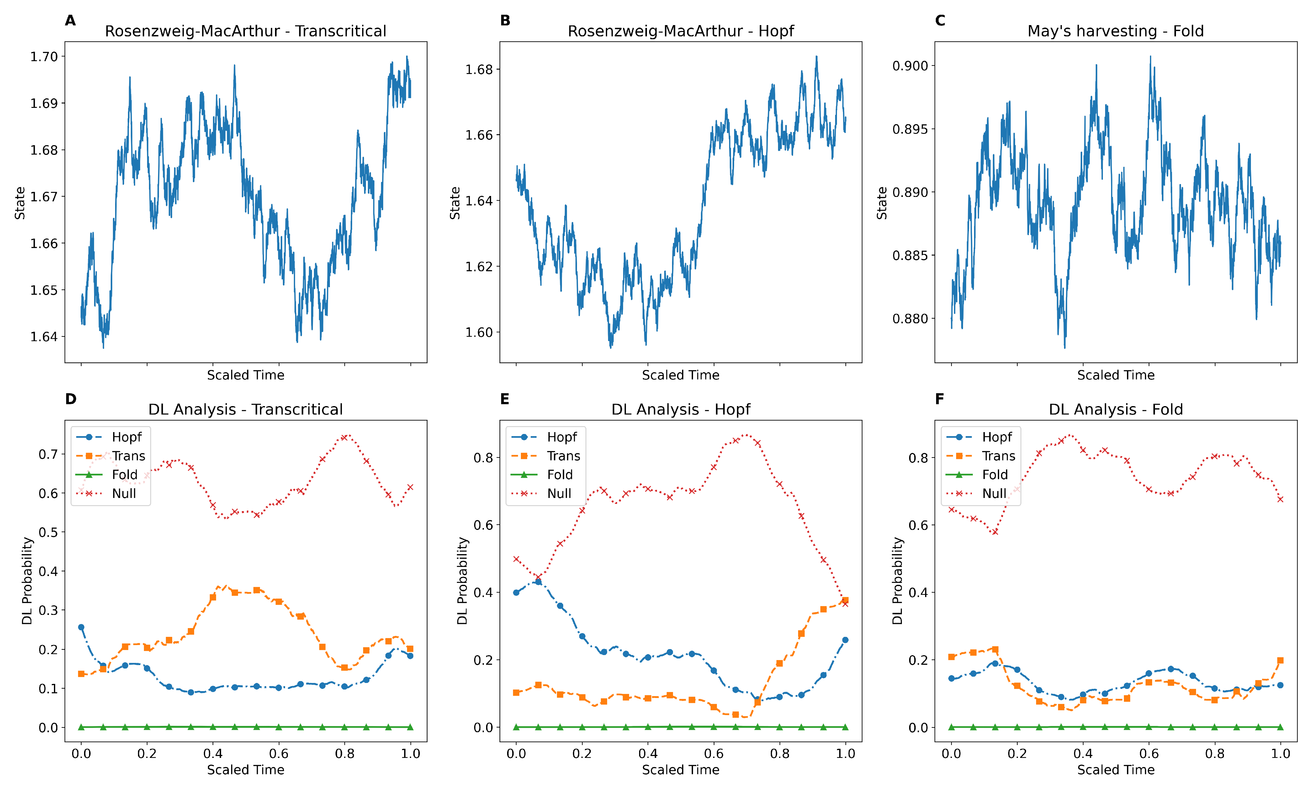
To evaluate the model’s ability to avoid false positives and correctly assign low confidence to bifurcation classes when no critical transition is present, we simulate time series from six nonlinear dynamical systems. In each case, control parameters are held fixed such that the system remains outside any bifurcation regime throughout the simulation. These represent purely null dynamics, meaning no tipping point occurs. This setup allows us to assess whether the classifier can reliably withhold predictions of bifurcations when presented with stable, non-transitioning systems—an essential capability for reducing false alarms in real-world applications.

• Bifurcating Systems:

• Rosenzweig–MacArthur Predator–Prey Model (Hopf or Transcritical):

  $${\displaystyle \frac{dx}{dt}}=rx\left(1-{\displaystyle \frac{x}{k}}\right)-{\displaystyle \frac{axy}{1+ahx}},{\displaystyle \frac{dy}{dt}}={\displaystyle \frac{eaxy}{1+ahx}}-my$$

  with the fixed parameters $r=4$, $k=1.7$, $e=0.5$, $h=0.15$, and $m=2$. For the transcritical bifurcation, the predation rate a is held constant at 6, and for Hopf it is held constant at 12.
• Fold Bifurcation Model (Harvesting):

  $${\displaystyle \frac{dx}{dt}}=x(1-x)-h·{\displaystyle \frac{x^2}{x^2+0.01}}$$

  where the harvesting rate h is held constant at 0.1 over the course of the simulation.
• Van der Pol Oscillator (Hopf):

  $${\displaystyle \frac{dx}{dt}}=y,{\displaystyle \frac{dy}{dt}}=\mu (1-x^2)y-x$$

  with $\mu =-7.0$.
• SIS Epidemic Model (Transcritical):

  $${\displaystyle \frac{dI}{dt}}=\beta I(1-I)-\gamma I$$

  where $\beta =4$, $\gamma =5$.
• Neural Activation Model (Fold):

  $${\displaystyle \frac{du}{dt}}=-u+{\displaystyle \frac{r}{1+exp(-5(u-1\left)\right)}}$$

  with $r=6$.

Null Dynamics: The null simulations are derived by fixing the control parameters in each system, preventing any bifurcation. For example, in the Rosenzweig–MacArthur model, $a=6$ is held constant to avoid crossing a bifurcation threshold. Similarly, in the fold and transcritical systems, the control parameters are set below the bifurcation point and remain unchanged throughout the simulation. The results are presented in Figure 7 and Figure 8.

5.4. Empirical Systems Used for Testing

In this paper, we have used two sources of empirical data to test the DL classifier.

• Sedimentary Archives (Mediterranean Sea)

This dataset provides high-resolution reconstructions of oxygen dynamics from sediment cores in the eastern Mediterranean Sea [52]. It captures transitions between oxic and anoxic states, with evidence of EWS preceding these transitions [53]. Data consist of molybdenum (Mo) and uranium (U) concentrations, proxies for anoxic and suboxic conditions, respectively, spanning eight anoxic events across three cores. A total of 26 time series are analyzed with a resolution of 10–50 years, depending on the core.

• Thermoacoustic Instability (Rijke Tube Experiments)

This dataset investigates transitions to self-sustained oscillations caused by thermoacoustic instability. Experiments were conducted in a horizontal Rijke tube with controlled voltage across a heated wire mesh to trigger transitions via subcritical Hopf bifurcations [54]. Data include 19 forced trajectories with varying voltage ramp rates and 10 steady-state trajectories at fixed voltages. Downsampled data (4 kHz or 10 kHz to 2 kHz) capture 1500 points prior to transitions.

Both datasets offer insights into detecting early signs of critical transitions in distinct physical systems.

5.5. Evaluation via ROC Curve Analysis

To assess the discriminative performance of our deep learning classifier in detecting early warning signals of bifurcations, we compute Receiver Operating Characteristic (ROC) curves across a range of simulated dynamical systems. Each system is configured to either gradually approach a bifurcation point (signal present) or remain in a stable regime with fixed parameters (signal absent). This binary labeling enables quantitative evaluation of the classifier’s ability to distinguish between pre-bifurcation and null dynamics.

Each time series is then classified using two CNN-LSTM models: one trained on white noise ($r=0$) and one trained on coloured (red) noise generated using an AR(1) process with varying auto-correlation levels ($r\in [0, 0.5]$). The model outputs softmax probabilities for four classes: transcritical, Hopf, fold, and null.

For ROC construction, we treat the mean probability of the correct bifurcation class as the classifier score. By sweeping over 200 thresholds $\tau \in [0, 1]$, we compute binary predictions at each level by classifying a window as “signal present” if the score exceeds $\tau$. The true positive rate (TPR) and false positive rate (FPR) are then defined as:

$$\mathrm{TPR}\left(\tau \right)={\displaystyle \frac{\mathrm{Correctly}\mathrm{classified}\mathrm{signal}\mathrm{windows}}{\mathrm{Total}\mathrm{signal}\mathrm{windows}}},\mathrm{FPR}\left(\tau \right)={\displaystyle \frac{\mathrm{Incorrectly}\mathrm{classified}\mathrm{null}\mathrm{windows}}{\mathrm{Total}\mathrm{null}\mathrm{windows}}}.$$

Varying the threshold $\tau$ traces out the ROC curve, revealing the sensitivity–specificity trade-off. To ensure robustness against stochasticity in simulation and training, this procedure is repeated over 50 Monte Carlo runs, and the resulting TPR and FPR values are averaged. The area under the ROC curve (AUC) is used to summarize performance: values close to 1 indicate strong discriminative ability, while values near 0.5 suggest random guessing. This evaluation is conducted separately for classifiers trained on white and red noise to compare their generalization under different noise structures.

5.6. Extended Evaluation of the DL Model Using Empirical Datasets

We evaluated the deep learning model on both experimental and geological datasets to demonstrate its ability to generalize from synthetic to empirical time series. Specifically, the analysis includes thermoacoustic transition signals from combustor experiments at ROF 3 and ROF 4, as well as geological anoxia indicators from sediment cores at site 64PE. Figure 9 shows the corresponding time series and the model’s bifurcation predictions.