Abstract
Accurate photovoltaic (PV) power output forecasting is critical for ensuring stable operation of modern power systems, yet it is constrained by high-dimensional redundancy in input weather data and the inherent heterogeneity of output scenarios. To address these challenges, this paper proposes a novel cascaded data-driven forecasting approach that enhances forecasting accuracy through systematically improving and optimizing the feature extraction, scenario clustering, and temporal modeling. Firstly, guided by weather data–PV power output correlations, the Deep Autoencoder (DAE) is enhanced by integrating Pearson Correlation Coefficient loss, reconstruction loss, and Kullback–Leibler divergence sparsity penalty into a multi-objective loss function to extract key weather factors. Secondly, the Fuzzy C-Means (FCM) algorithm is comprehensively refined through Mahalanobis distance-based sample similarity measurement, max–min dissimilarity principle for initial center selection, and Partition Entropy Index-driven optimal cluster determination to effectively cluster complex PV power output scenarios. Thirdly, a Long Short-Term Memory–Temporal Pattern Attention (LSTM–TPA) model is constructed. It utilizes the gating mechanism and TPA to capture time-dependent relationships between key weather factors and PV power output within each scenario, thereby heightening the sensitivity to key weather dynamics. Validation using actual data from distributed PV power plants demonstrates that: (1) The enhanced DAE eliminates redundant data while strengthening feature representation, thereby enabling extraction of key weather factors. (2) The enhanced FCM achieves marked improvements in both the Silhouette Coefficient and Calinski–Harabasz Index, consequently generating distinct typical output scenarios. (3) The constructed LSTM–TPA model adaptively adjusts the forecasting weights and obtains superior capability in capturing fine-grained temporal features. The proposed approach significantly outperforms conventional approaches (CNN–LSTM, ARIMA–LSTM), exhibiting the highest forecasting accuracy (97.986%), optimal evaluation metrics (such as Mean Absolute Error, etc.), and exceptional generalization capability. This novel cascaded data-driven model has achieved a comprehensive improvement in the accuracy and robustness of PV power output forecasting through step-by-step collaborative optimization.
Keywords:
distributed PV; PV power output forecasting; cascaded data-driven; key weather factors; output scenario MSC:
68T07
1. Introduction
To facilitate the achievement of the “carbon peak and carbon neutrality” targets, China is actively advancing the construction of a new power system dominated by photovoltaic (PV) and wind power, among other renewable energy sources [1]. However, PV power generation is susceptible to weather factors, exhibiting both strong intermittency and stochasticity, which poses significant challenges to the secure and stable operation of the power system. Accurate PV power output forecasting is of critical importance for power system optimization scheduling, efficient integration of renewable energy, and maintaining supply–demand equilibrium in electricity markets [2].
Based on differences in modeling principles, existing PV power output forecasting models are primarily categorized into physical models and data-driven models [3]. Physical models based on the mechanism of PV power generation achieve power output forecasting by analytically describing physical processes such as irradiance conversion and semiconductor characteristics. These models offer advantages including well-defined physical interpretability and reduced data dependency [4]. Ma Y et al. introduces an irradiance-corrected physical model, effectively enhancing forecasting accuracy in scenarios involving minor fluctuations like thin cloud cover [5]. Considering the irradiance mutation effect caused by cloud movement, Liu Q et al. establishes a dynamic correction model for cloudy weather by performing spatiotemporal matching of ground-based and satellite cloud images, significantly improving the model’s adaptability [6]. However, physical models often incorporate only a subset of weather factors during the modeling process, making it difficult to comprehensively capture PV power output variations under complex scenarios [7]. Data-driven models based on historical weather data typically employ statistical learning methods or deep learning techniques for PV power output forecasting. Among these, models based on statistical methods are predominantly linear, such as Autoregressive (AR) models [8], Autoregressive Integrated Moving Average (ARIMA) models [9], and Seasonal Autoregressive Integrated Moving-Average (SARIMA) models [10]). These offer advantages like relatively simple structure and ease of implementation. However, due to the significant nonlinear relationship between weather data and PV power output, the application of such models in PV power output forecasting is somewhat constrained. In recent years, forecasting models based on deep learning techniques have demonstrated considerable advantages in short-term PV power output forecasting (1–2 days timescale) [11]. Short-term forecasting with 15–30 min resolution, directly impacts the economic efficiency and security of day-ahead generation scheduling [12]. Among these models, Convolutional Neural Network (CNN) [13] and Recurrent Neural Network (RNN) [14] utilize their robust spatial feature extraction and data fitting capabilities to accurately model the complex weather data–PV power output relationship through multi-level nonlinear transformations. Jurado M et al. proposes a multi-layer CNN architecture that captures regional characteristics of cloud movement by spatially aligning satellite cloud images with Numerical Weather Forecasting (NWP) data, enhancing model accuracy in cloudy scenarios [15]. RNNs and their variants focus on modeling temporal dependencies. Utilizing the Long Short-Term Memory (LSTM) network, a variant of RNNs, Sabareesh et al. captures the temporal correlation between historical PV power output and irradiance data, improving the model’s capability to handle long-sequence data [16]. However, a single model struggles to characterize the spatio-temporal coupling characteristics of PV power output, thus hybrid models have become a research focus. Al-Ja’afreh et al. proposes a CNN–LSTM hybrid model, utilizing the CNN’s capacity for extracting local weather features alongside the LSTM’s temporal modeling capabilities, significantly enhancing forecasting performance under complex weather conditions [17]. However, this model architecture exhibits heightened complexity, necessitates larger volumes of training data and greater computation, and demonstrates heightened susceptibility to overfitting. Yang J et al. proposed a hybrid model leveraging ARIMA’s strong interpretability to forecast regular variation patterns in PV power output, while establishing a time-attentive LSTM to forecast irregular variation trends [18]. Although this hybrid model demonstrates significantly higher forecasting accuracy than individual models, its parameter specification (e.g., differencing order) requires iterative empirical determination. Zhu H et al. presents a hybrid PV power forecasting method based on Temporal Convolutional Network-Bidirectional Long Short-Term Memory (TCN-BiLSTM) [19]. It achieves efficient and accurate power forecasting by enhancing on-site data quality. But it takes a relatively long calculation time, and its generalization performance remains to be verified.
The accuracy of forecasting models based on deep learning techniques is highly dependent on the quality of input weather data [20]. High-dimensional redundant weather data and heterogeneous output scenarios constitute key challenges constraining the accuracy of PV power output forecasting models [21]. Regarding redundant weather data, if all these data are input directly into the forecasting model, it would likely lead to model overfitting and prolonged training times. Consequently, dimensionality reduction is required to extract key weather factors from the high-dimensional data. Existing research employs methods such as Principal Component Analysis (PCA), Grey Relational Analysis (GRA), and Deep Autoencoders (DAEs) to extract key weather features. For instance, PCA reduces weather data dimensionality to extract key weather factors, accelerating computational processes [22]. GRA identifies and selects weather factors strongly correlated with PV power output to enhance data efficacy [23]. However, both PCA and GRA rely on linear assumptions, fail to capture the nonlinear weather data–PV power output relationship [24]. In contrast, DAE has an additional layer with nonlinear activation, excels at nonlinear feature extraction, effectively denoising data while preserving critical information, and is suitable for complex large datasets [25,26,27]. Nevertheless, DAE focuses exclusively on minimizing reconstruction loss without explicit consideration of weather data–PV power output correlations, consequently yielding suboptimal feature representation. Regarding heterogeneous output scenarios, clustering methods such as K-means [28] and Fuzzy C-means (FCM) [29] are widely employed to generate typical PV power output scenarios. For instance, Das O et al. employs K-means method to generate typical scenarios (e.g., sunny, cloudy, rainy) for analyzing PV power output characteristics [30]. Yang M et al. proposes a weather type classification method based on the Elkan K-means algorithm that reuses historical features, thereby improving the day-ahead power forecasting accuracy [31]. As a hard clustering method, K-means assigns each data point exclusively to a single cluster. This renders the clustering results susceptible to distortion by anomalous data. In contrast, FCM, a fuzzy clustering method, permits partial membership across multiple clusters, thereby better capturing the continuous transitions inherent in PV power output behavior [32]. This method has been applied to cluster PV power output and NWP data, constructing physically coupled “weather data–PV power output” scenarios that improve clustering flexibility. Nevertheless, FCM implementation for PV power output forecasting faces three limitations: (1) Measurement on Euclidean distance neglects feature scaling differences, compromising scenario interpretability; (2) High sensitivity to initial cluster centroids frequently induces suboptimal convergence; (3) Manual determination of cluster numbers induces segmentation errors, limiting generalizability.
Considering the above, the purpose of this paper is to present a novel cascaded data-driven approach for PV power output forecasting to achieve multi-scenario adaptation and high forecasting accuracy. The research framework is illustrated in Figure 1. The modeling process comprises extracting key weather factors, clustering PV power output scenarios, and performing PV power output forecasting. Firstly, an enhanced DAE is developed, guided by weather data–PV power output correlation. This utilizes the nonlinear compression capabilities of the encoder and decoder to strip away redundant weather data, thereby extracting key weather factors strongly correlated with PV power output. Subsequently, an improved FCM clustering method is implemented. By optimizing the inter-sample distance, initial cluster centroids, and the number of clusters, this generates significantly distinct typical PV power output scenarios. Finally, dedicated LSTM models are constructed for each output scenario. These utilize gated mechanisms and a temporal pattern attention mechanism to learn the time-series relationships between key weather factors and PV power output within each specific scenario, ultimately enabling PV power output forecasting. The main research contributions of this paper are as follows.
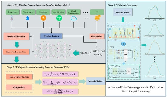
Figure 1.
Research framework.
- (1)
- An enhanced DAE is designed guided by weather data–PV power output correlations. By incorporating the Pearson Correlation Coefficient (PCC) alongside reconstruction loss and KL divergence penalty, a multi-objective loss function is constructed. This effectively filters noise and redundant information within high-dimensional weather data while capturing nonlinear interaction effects among weather factors such as irradiance and temperature through nonlinear encoding. Consequently, it achieves dimensionality reduction for extracting critical weather factors strongly correlated with PV power output from multidimensional weather factors, thereby providing high-quality input features for subsequent scenario clustering modeling.
- (2)
- An improved FCM is proposed for complex PV power output scenario clustering. This approach employs the Mahalanobis distance (MD) to measure sample similarity, utilizes the max–min dissimilarity principle for rapid initial cluster center selection, and implements partition entropy (PE) index-based optimization for determining the optimal cluster number. These innovations enable the rapid and precise subdivision of extracted low-dimensional key weather factors into multiple sets of typical weather scenarios. Consequently, the subsequent LSTM–TPA forecasting model can adaptively adjust forecasting weights according to each scenario’s characteristics, establishing a scenario-aware forecasting model.
- (3)
- A cascaded data-driven forecasting framework is systematically constructed, integrating key weather factor extraction, precise scenario clustering, and temporal modeling. Through stage-wise collaborative optimization, this approach achieves comprehensive enhancement in both forecasting accuracy and robustness for PV power output.
The rest of this paper is organized as follows. Section 2 presents the extraction model of key weather factor-enhanced DAE. Section 3 details the scenario clustering model-enhanced FCM. The forecasting model is described in detail in Section 4. Section 5 presents experimental results. Finally, Section 6 concludes this paper.
2. Key Weather Factors Extraction Based on Enhanced DAE
The PV power output forecasting relies on future weather data, such as parameters including irradiance and ambient temperature, generated by NWP models. However, the multi-dimensional weather data generated by NWP exhibit redundant correlations and weakly correlated noise. If all these data are input into the forecasting model, this will lead to model overfitting and prolonged training time. However, exclusively considering strongly correlated factors while completely neglecting weakly relevant factors would conversely degrade prediction accuracy. While DAEs can extract key weather factors from these data, they may simultaneously incorporate information that is irrelevant to PV power output or characterized by highly redundant features. This section presents improvements to standard DAE by constructing a multi-objective loss function which incorporates a PCC loss function LPCC, a reconstruction loss function LMSE, and a Kullback–Leibler (KL) divergence-based sparsity penalty loss function Ls. Consequently, the extraction of key weather factors is effectively guided by the correlation between weather data and PV power output. Thereby achieving mitigation of data redundancy, prevention of overfitting, and enhancement of model training efficiency.
2.1. Structure of DAE
DAE is an unsupervised multi-layer neural network model comprising two components: an encoder and a decoder [25]. This structure enables the feature extraction and data dimensionality reduction through its encoding-decoding mechanism, as illustrated in Figure 2. The encoder compresses the original data into a low-dimensional latent space via nonlinear mapping, while the decoder reconstructs the output data from the latent features . The encoding and decoding processes are expressed as follows:
where f is the nonlinear activation function, and are the trainable parameters of the encoder and decoder, respectively.
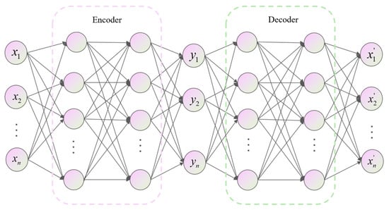
Figure 2.
DAE structure.
2.2. Design of Multi-Objective Loss Function
Firstly, LPCC is constructed to maximize the average correlation between all hidden-layer features and PV power output. The hidden-layer feature matrix is defined as , where n is the sample size and k is the latent feature dimension. The PV power output sequence is denoted as . The PCC between the jth hidden feature Yj and output PPV is then given by [33]:
where Yj,i is the value of the jth hidden feature on the ith sample, is the average value of the jth hidden feature samples, is the average value of the PV power output sequence samples.
The PCC ranges between [−1, 1], where a value of 0 denotes no correlation between variables, 1 indicates a strong positive correlation, and −1 signifies a strong negative correlation, with higher absolute values corresponding to stronger degrees of association.
LPCC is defined as:
Secondly, Ls is adopted to further reduce redundant features within the data. It is defined as [25]:
where β is the penalty coefficient, e is the number of neurons in the hidden layer, ρ is the preset sparsity target, ρg is the average activation value of the gth hidden layer neuron across all samples.
Thirdly, LMSE is formulated by constraining the discrepancy between the decoder’s input and output. This ensures the model achieves a high-fidelity encoding of the original data features. It is defined as [25]:
where and are the original weather data and the reconstructed weather data of the ith sample, respectively.
Finally, the correlation loss function LPCC, sparse penalty loss function Ls and reconstruction loss function LMSE are integrated to form a multi-objective loss function Ltotal:
where , and are the weight coefficients of each function, respectively.
2.3. Determination of Intrinsic Dimension
Intrinsic dimensionality characterizes the compactness of the data distribution after dimensionality reduction. Its selection directly influences the effectiveness of feature extraction: an excessively large intrinsic dimension retains redundant information, while an overly small one risks the loss of critical feature information. This paper employs the reconstruction fidelity D(a) of latent features to optimize the intrinsic dimensionality of key weather factors. The specific steps are as follows:
- Set the initial intrinsic dimension a is 1, and define the maximum candidate dimension is amax;
- Calculate D(a) for each candidate dimension as follows [25]:
- 3.
- Traverse all candidate dimensions a, calculate D(a), and select the dimension corresponding to the curvature drop point as the optimal intrinsic dimension k.
This approach quantifies the reconstruction error with varying dimensions, thereby balancing the trade-off between dimensionality reduction and information retention.
3. PV Output Scenario Clustering Based on Enhanced FCM
As previously discussed, the FCM clustering method suffers from three limitations: failure to account for dimensional disparities in sample data, time-consuming selection of initial cluster centers, and the necessity for manual intervention in determining the number of clusters. Applying this method may yield PV power output scenarios that deviate from actual distribution characteristics, thereby compromising the representativeness of the typical scenario. To address these issues, this section proposes an enhanced FCM clustering method for PV power output scenario clustering.
3.1. Similarity Measurement Reformulation Based on Mahalanobis Distance
FCM employs a similarity measure based on Euclidean distance (ED), which assumes that all features are mutually independent and equally weighted. However, in the clustering of PV power output scenarios, even after extracting key weather factors via DAEs, dimensional disparities between features persist. The MD is introduced to replace ED as the metric for sample similarity measurement. The MD eliminates dimensional disparities between features through the inverse of the covariance matrix and adaptively adjusts the weighting of each feature. Thereby, it provides a more accurate measure of similarity between samples. The distance between samples is calculated as follows [34]:
where , are different samples, is the covariance matrix of weather data.
3.2. Initial Clustering Center Selection Based on Max–Min Distance
To enhance clustering efficiency and strengthen the representativeness of the initial centers, an initial cluster center selection strategy based on the max–min dissimilarity principle is employed. This strategy first performs targeted selection of highly dissimilar samples as initial centers. This reduces the number of iterations while simultaneously mitigating the risk of local optima resulting from random initialization of cluster centers. Furthermore, by integrating MD, the initial cluster centers are enabled to both characterize the key distribution patterns of weather factors and accommodate the power–output-oriented clustering requirements. The specific procedure is outlined as follows:
- Step 1: Randomly select NB samples from the key weather factor dataset as clustering center, and place them into the initial candidate center set Z.
- Step 2: Iterate through the remaining samples N\Z. For each sample xj, calculate the total MD to the current candidate cluster center set Z.
Following the Maximum–Minimum Dissimilarity Principle, select the sample exhibiting the greatest distance to existing centers and add it to set Z.
- 3.
- Step 3: Repeat Step 2 until the number of candidate centers reaches the predefined clustering number T. Subsequently, calculate the equivalent distance Dt between the current candidate center set Z and the remaining sample set N\Z.
If the change in equivalent distance between consecutive iterations falls below a preset convergence threshold , terminate the iteration and output the initial cluster center set Z.
Subsequent clustering is executed via the FCM algorithm, with implementation details referenced from [35].
3.3. Adaptive Cluster Number Determination Based on Partition Entropy Index
To eliminate the error arising from the manual specification of the cluster number in FCM, an adaptive cluster number selection method based on the PE Index is adopted. This method identifies the optimal number of clusters by quantifying the degree of disorder within the membership distribution. The PE is defined as follows [36]:
where the value range of PE is 0 to logT, T is the current clustering number with a value range of 2 to Tmax, Tmax is the maximum clustering number, typically set as ( is the ceiling operation), ujt is the membership degree of the jth sample to the tth clustering center.
The relationship between the clustering number T and PE is shown in Figure 3. As T increases, the PE increases simultaneously, resulting in clearer clustering. Conversely, a lower PE corresponds to harder clustering. Selecting the optimal number of clusters requires balancing cluster clarity against cluster hardness. Generally, the number of clusters corresponding to the points with a significant increase in curve curvature is the optimal number of clusters.
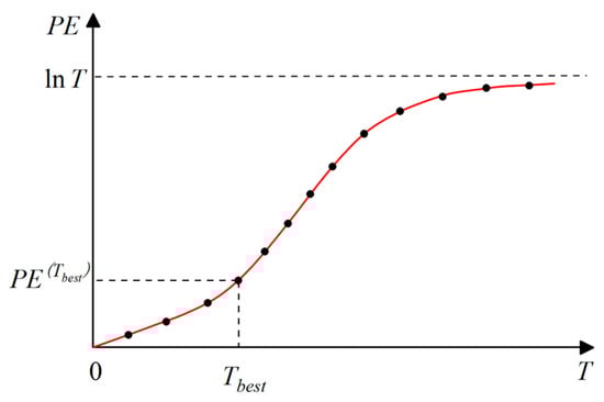
Figure 3.
T–PE relationship.
4. PV Output Forecasting Model
Conventional forecasting models typically employ a global mapping approach. This method is scenario-insensitive and struggles to capture the differential evolution of the “weather data–PV power output” relationship across varying output scenarios. This section integrates the LSTM model with the Temporal Pattern Attention (TPA) mechanism to construct scenario-specific temporal forecasting models. This structure implements a coordinated scenario-localization principle, adaptively learning salient scenario-specific patterns to precisely characterize inherent scenario-dependent variations in PV power output forecasting.
4.1. Fundamentals of LSTM Network
LSTM, a specialized recurrent architecture, process temporal data via gated cells that selectively retain and expose information [14]. Each cell contains three regulatory gates (input/forget/output) controlling cell state propagation, as shown in Figure 4. The network comprises temporally recurrent, parametrically identical units.
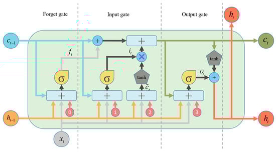
Figure 4.
Structure of the LSTM cell.
At timestep t, each LSTM cell processes the input and the previous hidden state to generate: (1) the new cell state , which functions as the primary memory repository for information storage and propagation; (2) the current hidden state ; (3) the output . Three gating signals, the forget gate , the input gate , and the output gate , collectively regulate information flow through to enable precise long-term dependency modeling. Specifically, the forget gate computes retention weights from and to attenuate segments of ; the input gate selectively integrates candidate memory derived from and into the cell state; and the updated emerges from the element-wise summation of the attenuated prior state and gated new memory. Finally, the output gate modulates to produce , which simultaneously serves as the timestep output and propagates to the next cell. The process are as follows:
where , , are the weight matrices linking the previous hidden state to the forget, input, and output gates, respectively, , , are the weight matrices linking the current input to each gate, , , are bias vectors associated with each gate. , are the weight matrices with and , respectively, is the bias vector associated with , signifies element-wise multiplication.
The activation function for LSTM employs the sigmoid function, defined as:
This function provides bounded derivatives for stable gradient flow during backpropagation, with outputs constrained to [0, 1] to regulate information gating.
Throughout this process, and jointly modulate gating signals, enabling adaptive integration of current inputs with historical context. The hidden state serves dual roles: (1) as the current output and (2) as the propagated latent representation to the next timestep. The cell state evolves longitudinally, with gated local adjustments balancing long-term memory retention and short-term input assimilation.
4.2. Principles of TPA Mechanism
TPA, a feature enhancement architecture specifically designed for sequential data, dynamically amplifies model sensitivity to critical temporal features through adaptive weight allocation. TPA focuses critical temporal patterns through cascaded multi-scale feature extraction and attention-based weighting. Its structural schematic is presented in Figure 5 [37].
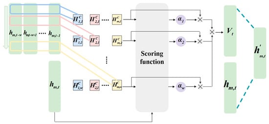
Figure 5.
Structure of TPA mechanism.
As depicted in Figure 5, at initial stage, it applies multi-scale temporal convolution to the LSTM hidden state matrix , where T is total timesteps, m is hidden dimension. This operation utilizes k variable-length 1D convolutional kernels , where dj is the length of the jth kernel. This convolution generates a multi-scale feature matrix with elements computed as:
where t is the current timestep index, is the kernel sliding position index, is the full hidden state vector at step , and is the weight at position of the jth kernel.
Subsequently, it performs dynamic feature weighting by treating the current hidden state as the query vector and as key-value pairs. The relevance score is computed as:
where is the ith row vector of , and is the learnable attention matrix.
During training, adaptive adjustment of query–key interactions enables differential focus on distinct temporal patterns, particularly effective for modeling nonlinear time-dependent relationships between weather factors and PV power output generation. The Softmax function maps scores to attention weights reflecting the contribution of the ith timestep’s features to current forecasting:
The context vector , integrating temporal features, is generated by the weighted summation of the temporal pattern matrix with attention weights :
The original hidden state and are concatenated into a joint representation, which undergoes feature fusion through a fully connected layer to produce the enhanced hidden state :
where is the learnable weight matrix for linear transformation.
4.3. Integrated LSTM–TPA Model
The integrated LSTM–TPA unit, as shown in Figure 6, combines LSTM’s temporal dependency modeling with TPA’s adaptive attention weighting. Specifically, the LSTM captures sequential dependencies in output generation data. The TPA module dynamically allocates attention weights to key weather factors across historical timesteps, enhancing sensitivity to key weather features. The TPA module, at the model’s output layer, dynamically adjusts historical information weighting through a three-stage processing. Firstly, the hidden state matrix from all timesteps of the LSTM serves as the input substrate. Subsequently, trainable parameter matrices compute relevance scores between the current timestep state and each historical state, converting these into normalized attention weights. Finally, these weights dynamically fuse historical states through weighted integration, generating a temporally aware context vector. This context vector is then concatenated with the current hidden state, collectively contributing to the final forecasting output.
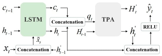
Figure 6.
Integrated LSTM–TPA model.
Specially, The inputs are the current weather factors vector , the prior cell state , the hidden state , the TPA-optimized hidden state ,and the historical hidden state matrix . Crucially, the LSTM input replaces raw features with an augmented vector , enabling joint utilization of real-time weather data and attention-refined historical context. This design reinforces temporal continuity by propagating attention-filtered information. The LSTM updates its cell state and hidden state via gating mechanisms. These states are concatenated into an attention query vector , to drive TPA’s weight computation. The final forecasting result is generated through a ReLU-activated output layer.
This method adaptively allocates attention weights, eliminating rigid dependence on uniform temporal sampling to precisely identify critical periods influencing PV generation. Furthermore, the optimized hidden state propagates recursively across timesteps, establishing a closed-loop memory–attention enhancement mechanism. This dual-path design preserves the LSTM’s intrinsic capacity for the temporal dependency model, and augments state representations via attention-guided refinement, thereby increasing informational richness of hidden states and ultimately enhancing forecasting accuracy.
5. Results and Discussion
To validate the effectiveness of the proposed approach, this section utilizes PV cluster data and weather information for the Konstanz region in Germany, the coordinate position is 47.68° N latitude and 9.18° E longitude, provided by the International Solar Energy Research Center (ISC) [38] and Solcast [39]. The total installed capacity of the PV cluster is 5.7 MW, comprising ten distributed PV power plants with capacities of 0.6, 0.4, 0.8, 0.5, 0.7, 0.9, 0.3, 0.6, 0.4, and 0.5 MW, respectively. Data samples were collected at 30 min intervals from 1 January 2016 to 31 December 2017. The weather dataset encompasses 14 factors, including air temperature, surface albedo, irradiance and so on. For the handling of missing or anomalous weather data, this paper first identifies and removes outliers using the 3-σ criterion. Subsequently, missing data completion is performed: for data missing over continuous periods, linear interpolation is employed; for discrete missing data points, mean imputation using data from adjacent time points is applied. Furthermore, accounting for the temporal correlation inherent in weather data, interpolation is conducted using a weighted calculation incorporating data from five preceding and subsequent timesteps.
A randomly selected 15% of the data samples constitute the test set, with the remaining samples used for training. During model training, the process is terminated if no significant decrease in training loss is observed over 20 consecutive iterations. The model parameters corresponding to the minimum observed loss are then considered optimal.
All computational workflows executed within PyCharm 2023.2.1 and TensorFlow-GPU 2.4.0. Model hyperparameters were optimized using the grid search method, with the optimal combination selected via five-fold cross-validation within predefined ranges. The primary configurations for each module are as follows:
- (1)
- DAE: Four-layer encoder and three-layer decoder architecture; target sparsity rate: 0.05; activation function: sigmoid.
- (2)
- LSTM: Single LSTM layer; number of hidden units: 120.
- (3)
- TPA: Temporal window length: 3; dimensions of the attention matrix: 120 × 8.
To verify the suitability of the employed data samples, this study utilizes the PCC to analyze the correlation between weather factors and PV power output. Data from seven consecutive days were randomly selected from the dataset to compute the PCC, with their average value taken. The results are presented in Figure 7.
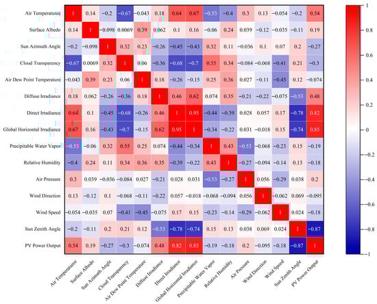
Figure 7.
Correlation between weather factors and PV power output.
As we can see in Figure 7, PV power output exhibits a stronger positive correlation with irradiance and air temperature; a weaker negative correlation with precipitable water content and wind speed; and a relatively weak correlation with solar azimuth angle, while demonstrating a stronger negative correlation with solar zenith angle. These observed correlations align consistently with established physical principles. Consequently, the weather dataset is deemed reasonable and suitable for PV power output forecasting.
5.1. Evaluation Metrics
To evaluate the performance of the forecasting model, this study employs multiple metrics: Mean Absolute Error (MAE), normalized Mean Absolute Error (nMAE), Root Mean Square Error (RMSE), normalized Root Mean Square Error (nRMSE), and the Coefficient of Determination (R2). The calculation formulae for these metrics are as follows:
where and denote the actual value and forecasting value, respectively, represents the sample size, is the average value of sample, and indicates the PV capacity.
Furthermore, to evaluate the effectiveness of the scenario clustering, this study employs the Silhouette Coefficient (SC) and the Calinski–Harabasz Index (CHI) as evaluation criteria [40]. Additionally, the computation time is recorded to analyze clustering efficiency. The SC measures the appropriateness of sample assignments to clusters, while the CHI reflects the compactness and separation of the cluster structure. Combining both metrics enables a comprehensive assessment of clustering performance. The formulae for SC and CHI are defined as follows:
where is the SC of sample , is the average distance between sample and other samples within the same cluster, is the average distance between sample and samples within the nearest cluster, and is the total number of samples. , the value approaching 1 indicate well-separated clusters with high intra-cluster cohesion, whereas values near −1 suggest potential misassignment of samples to irrelevant clusters.
where is the inter-cluster dispersion, is the intra-cluster dispersion, is the number of cluster centroids, and denotes the number of samples and the centroid of the gth cluster, respectively, represents the global centroid of all samples, refers to a sample in the gth cluster, and is the set of samples in the gth cluster.
5.2. Validation of Enhanced DAE
With NWP data employed, the relationship between latent dimensionality and reconstruction fidelity , obtained via the intrinsic dimensionality optimization method established in Section 2.3, is presented in Figure 8. It indicates that the optimal intrinsic dimension k is 6.
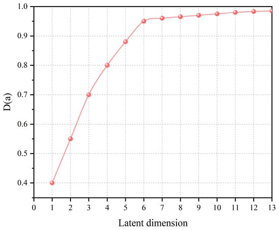
Figure 8.
Relationship between latent dimensionality and reconstruction fidelity.
Subsequently, the effectiveness of the enhanced DAE for extracting key weather factors is validated. Weather factors extracted from the NWP data using manual selection, PCA selection, the standard DAE, and the enhanced DAE are fed into the LSTM forecasting model. The resulting PV forecasting power outputs are illustrated in Figure 9, while the corresponding forecasting errors are detailed in Table 1.
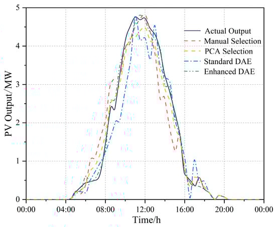
Figure 9.
Comparison of the effects of extracting key weather factors.

Table 1.
Comparison of evaluation metrics of extracting key weather factors.
As illustrated in Figure 9, the PV power output forecasting using the enhanced DAE exhibits significantly closer alignment with the actual power output compared to forecasting derived from manual selection, PCA selection and the standard DAE. This improvement is particularly pronounced during peak and trough generation periods. Further analysis of Table 1 reveals that the enhanced DAE achieves substantial performance gains: relative to manual selection, PCA selection, and the standard DAE, MAE reduces from 15.898%, 16.782%, and 19.567% to 9.972%, RMSE reduces from 18.606%, 20.261%, and 22.493% to 11.141%, while R2 increases from 91.602%, 89.581%, and 87.482% to 93.564%, respectively. These results demonstrate the superior predictive performance of the enhanced DAE.
This improvement in forecasting performance is directly attributable to the optimization of the multi-objective loss function. compels the encoder to extract key weather features that exhibit a high degree of linear correlation with variations in power output, the model enhances the representation of dynamic behavior in the output. Furthermore, refines sparse features with high information density by suppressing redundant activation within the hidden layers, thereby effectively reducing noise interference. The synergistic effect of these combined loss functions enables the model to accurately capture the core weather drivers while simultaneously filtering out irrelevant information. As a result, both forecasting accuracy and model robustness are substantially improved.
5.3. Validation of Enhanced FCM
To validate the effectiveness of the enhanced FCM, this section performs scenario clustering on the 6-dimensional weather features extracted by the enhanced DAE. The optimal number of clusters, determined by the adaptive cluster number determination method established in Section 3.3, is 5. Based on this optimal cluster number, the comparative clustering performance results among the enhanced FCM, K-means, and standard FCM are presented in Table 2.
Table 2.
Comparison of clustering performance metrics.
As shown in Table 2, in terms of both SC and CHI, the enhanced FCM (SC 0.73, CHI 1586) outperforms both K-means (SC 0.62, CHI 1250) and standard FCM (SC 0.65, CHI 1324). The improvement in the SC validates the effectiveness of the MD in enhancing intra-cluster consistency and inter-scenario distinguishability. Concurrently, the elevation in CHI reflects the enhanced discriminative capability of the enhanced FCM for complex PV power output scenarios. Regarding computational efficiency, while the enhanced FCM (8.2 s) is marginally inferior to K-means (5.1 s), it achieves a substantial reduction of 39.7% compared to the standard FCM (13.6 s), resulting in significantly diminished clustering iteration times. The enhanced FCM achieves a balance between clustering quality and computational efficiency.
To validate the effectiveness of the scenario clustering produced by the enhanced FCM, the clustered PV power output scenario dataset is utilized to train the LSTM forecasting model. The forecasting results are illustrated in Figure 10, while the corresponding evaluation metrics are presented in Figure 11.
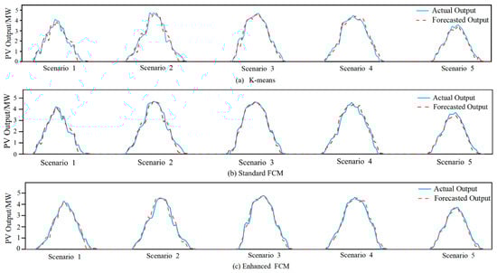
Figure 10.
Comparison of clustering performance in each scenario (a) K-means, (b) Standard FCM, (c) Enhanced FCM.
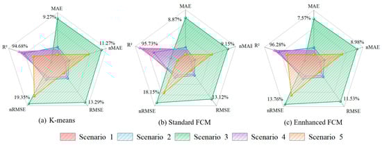
Figure 11.
Comparison of clustering evaluation metrics in each scenario (a) K-means, (b) Standard FCM, (c) Enhanced FCM.
As illustrated in Figure 10, for all scenarios, the PV power output forecasted using the enhanced FCM exhibits exceptional concordance with the actual output, significantly outperforming both K-means and standard FCM. This is particularly evident during peak generation periods, demonstrating superior tracking capability. Further analysis of Figure 11 confirms that the enhanced FCM achieves optimal evaluation metrics across all scenarios. For instance, in Scenario 3, the enhanced FCM yields an nRMSE as low as 13.76%, while the R2 reaches 96.2%, providing robust confirmation of the high congruence between forecasting values and actual values. This demonstrates that weather scenarios formed by the enhanced FCM clustering method more accurately drive the LSTM model to forecast PV power output across diverse scenarios. This enhanced capability stems primarily from the dual optimization mechanisms inherent to the enhanced FCM: (1) The MD metric effectively adapts to the correlations within high-dimensional weather features, thereby ensuring the clustered scenarios align closely with actual PV power generation patterns. (2) The optimized initial center selection strategy mitigates scenario boundary ambiguity inherent in standard FCM, thus enhancing clustering stability. The synergistic interaction of these mechanisms ensures the physical plausibility of the weather data–PV power output mapping relationships input into the forecasting model. This is ultimately manifested in comprehensive improvements to both tracking capability and forecasting accuracy.
5.4. Validation of Proposed Method
To verify the effectiveness of the TPA mechanism for PV power output time-series modeling, this section compares the proposed LSTM–TPA model against the standard LSTM model under the aforementioned input conditions. Furthermore, to validate the superior performance of the proposed cascaded forecasting approach, comparative analyses are conducted against CNN–LSTM [17] and ARIMA–LSTM [32]. The PV forecasting power outputs for each model are illustrated in Figure 12, while detailed performance evaluation metrics are presented in Table 3.
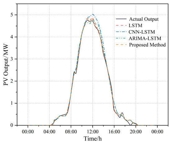
Figure 12.
Comparison of PV output forecasting.
Table 3.
Comparison of evaluation metrics of PV output forecasting.
As illustrated in Figure 12, the PV power output forecasted by the standard LSTM model generally aligns with the actual power output but exhibits discernible deviations at peak generation points and certain inflection points, indicating limitations in capturing fine-grained temporal details. The output predicted by the CNN–LSTM model demonstrate considerable volatility, exhibiting notable instability during certain morning and afternoon periods. While the ARIMA–LSTM model performs adequately during stable operational periods, its forecasting results exhibit lagged responses during steep output ramps or dips. In contrast, the PV power output forecasted by the proposed LSTM–TPA method exhibits the closest temporal alignment with the actual output. This superiority is particularly pronounced during peak output periods and dawn/dusk transition periods, demonstrating marked superiority over alternative models. Further analysis of Table 3 confirms the optimal performance of LSTM–TPA across all key metrics: It achieves the lowest values for MAE, nMAE, RMSE, and nRMSE, signifying superior overall error minimization and enhanced control over larger forecasting errors. It attains the highest R2, indicating the best model fit. Specifically, compared to the standard LSTM, LSTM–TPA achieves a 16.5% reduction in MAE, a 13.7% reduction in RMSE, and a 2.75% increase in R2, validating the efficacy of the TPA mechanism. Compared with the CNN–LSTM and ARIMA–LSTM models, the proposed method reduced the MAE by 39.7% and 25.8%, respectively, and the RMSE by 45.5% and 31.2%, respectively. Concurrently, the R2 significantly increased from 93.453% and 94.566% to 97.986%. These results strongly indicate the superiority of the cascaded data-driven approach, exhibiting a substantial overall advantage.
The following further verifies the effectiveness of the proposed approach for different seasons. The evaluation metrics for different season are shown in Table 4.
Table 4.
Comparison of evaluation metrics of PV output forecasting in different season.
The approach achieves optimal accuracy in summer (MAE 2.874%, RMSE 3.631%, R2 98.452%) when solar resources are most abundant, and exhibits slightly reduced but still remarkable performance in winter (MAE 4.231%, RMSE 5.134%, R2 95.885%) when cloud cover and irradiance variability pose the greatest challenges. For the transitional seasons of spring and autumn, the forecasting performance lies between that of summer and winter (R2 are 97.371% and 96.236% in spring and autumn, respectively), which is in perfect agreement with the gradual process of sunshine duration and weather patterns. This approach maintained excellent forecasting performance (R2 > 95.885%) in all seasons and consistent performance across seasons (ΔR2 < 1.5%), further confirming the effectiveness, stability and robust adaptability of the proposed approach under different weather conditions.
5.5. Validation of Forecasting Model Generalization Capability
This section assesses the generalization performance of the proposed cascaded data-driven approach by employing it to forecast the PV power output of ten distributed PV plants within the PV cluster. The forecasting output and performance evaluation metrics are depicted in Figure 13 and Figure 14, respectively.
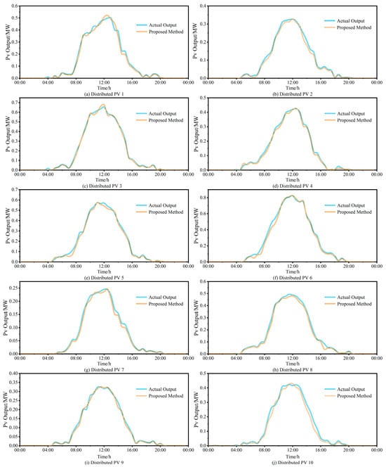
Figure 13.
Comparison of PV output forecasting for each distributed PV station (a) Distributed PV 1, (b) Distributed PV 2, (c) Distributed PV 3, (d) Distributed PV 4, (e) Distributed PV 5, (f) Distributed PV 6, (g) Distributed PV 7, (h) Distributed PV 8, (i) Distributed PV 9, (j) Distributed PV 10.
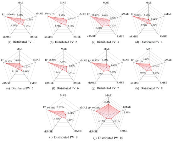
Figure 14.
Comparison of evaluation metrics of PV output forecasting for each distributed PV station (a) Distributed PV 1, (b) Distributed PV 2, (c) Distributed PV 3, (d) Distributed PV 4, (e) Distributed PV 5, (f) Distributed PV 6, (g) Distributed PV 7, (h) Distributed PV 8, (i) Distributed PV 9, (j) Distributed PV 10.
As observed in Figure 13, the proposed approach exhibits exceptional tracking capability for all ten distributed PV plants throughout the daily operation, maintaining robust tracking even during peak output periods. Further analysis of Figure 14 reveals consistently superior performance metrics across all plants: MAE values range between 2.63% and 3.59%, with eight plants achieving below 3.24% and plant PV4 attaining an optimal value of 2.63%. RMSE values fall within 2.97% to 4.03%, with eight plants below 4%. R2 values exceed 97% for all plants. These metrics collectively demonstrate that the predicted PV power output aligns closely with actual measurements across all installations. The results conclusively validate the exceptional generalization capability of the proposed approach.
6. Conclusions
This study proposes a cascaded data-driven approach for PV power output forecasting. By optimizing three sequential stages of feature extraction, scenario clustering, and temporal modeling, the approach significantly enhances forecasting accuracy. Based on the case study results, the following conclusions are drawn:
- (1)
- The enhanced DAE, guided by weather data–PV power output correlations, integrates the , , and into a multi-objective loss function. Compared to manual feature selection, PCA selection, and standard DAE, PV power output predicted by the enhanced DAE exhibit exceptional concordance with actual PV power output. Key evaluation metrics MAE and RMSE show substantial reductions (MAE 9.972% and RMSE 11.141%), while R2 demonstrates significant improvement (93.564%), confirming superior forecasting accuracy. The enhanced DAE effectively extracts key weather factors strongly correlated with PV power output, establishing a robust data foundation for subsequent modeling.
- (2)
- The enhanced FCM employs the MD to accurately measure dissimilarities between weather samples. Utilizing the max–min dissimilarity principle expedites initial cluster center selection, enhancing efficiency and representativeness. An adaptive cluster number selection method, based on the PE, identifies the optimal cluster number 5. In terms of clustering effectiveness, the enhanced FCM outperforms both K-means and standard FCM, achieving marked improvements in SC (0.73) and CHI (1586). This enables effective distinction and identification of complex PV power output scenarios while reducing clustering iteration time (8.2 s). Regarding predictive performance, the enhanced FCM yields optimal evaluation metrics (such as MAE 7.57%, RMSE 11.3%, and R2 96.2 for Scenario 3) and demonstrates superior output tracking against actual data, particularly during peak generation periods. Consequently, the weather scenarios clustered by the enhanced FCM more precisely drive the LSTM model’s responsiveness across diverse scenarios.
- (3)
- The constructed LSTM–TPA model utilizes gating mechanisms and TPA to learn the time-series patterns linking key weather factors and PV power output within each scenario. Forecasting output from this model align more closely with actual output, especially during power peaks and inflection points, demonstrating superior capability in capturing fine-grained temporal details compared to the standard LSTM model.
- (4)
- Compared to CNN–LSTM and ARIMA–LSTM, the proposed cascaded data-driven approach achieves significantly closer alignment between forecasting output and actual output. It attains optimal values across all key metrics: yielding the lowest MAE (3.171%), nMAE (3.283%), RMSE (3.538%), and nRMSE (3.672%, signifying superior overall error minimization and control over larger deviations), alongside the highest R2 (97.986%, indicating optimal model fit). The approach’s exceptional generalization capability is further validated by its accurate forecasting across ten distributed PV plants within a PV cluster.
Through the staged optimization of feature extraction, scenario clustering, and scenario-specific modeling, a preliminary verification of the weather data and PV output data of the Konstanz region in Germany is conducted. This dataset is rich in weather factors. The proposed cascaded data-driven PV power output forecasting approach achieves comprehensive improvements in both forecasting accuracy and robustness, providing a reasonable benchmark for the performance verification of the model under complex weather conditions. However, this approach still has a relatively strong dependence on the quality of input data. Whether it is applicable to output forecasting for datasets from other PV power plants or new energy plants remains to be further researched in future work.
Author Contributions
Conceptualization, C.X. and T.Y.; Data curation, W.L.; Formal analysis, C.X.; Investigation, X.L.; Methodology, C.X. and X.L.; Resources, X.L.; Software, X.L. and W.L.; Supervision, T.Y.; Validation, C.X. and X.L.; Visualization, X.L.; Writing—original draft, C.X. and X.L.; Writing—review and editing, C.X. and X.L. All authors have read and agreed to the published version of the manuscript.
Funding
This work was supported by the National Key Research and Development Program of China under grant number 2023YFB4301500, and the Opening Foundation of Shanghai Ship and Shipping Research Institute Co., Ltd. under grant number W23CG000116.
Data Availability Statement
The original contributions presented in this study are included in the article. Further inquiries can be directed to the corresponding author.
Conflicts of Interest
Author Xiang Liu was employed by the Jinhua Power Supply Company and Wei Liu was employed by the company Shanghai Ship and Shipping Research Institute Co. The remaining authors declare that the research was conducted in the absence of any commercial or financial relationships that could be construed as a potential conflict of interest.
References
- Joshi, P.; Rao, A.B.; Banerjee, R. Review of solar PV deployment trends, policy instruments, and growth projections in China, the United States, and India. Renew. Sustain. Energy Rev. 2025, 213, 115436. [Google Scholar] [CrossRef]
- Zheng, F.; Meng, X.; Wang, L.; Zhang, N. Operation optimization method of distribution network with wind turbine and photovoltaic considering clustering and energy storage. Sustainability 2023, 15, 2184. [Google Scholar] [CrossRef]
- Ahmed, R.; Sreeram, V.; Mishra, Y.; Arif, M.D. A review and evaluation of the state-of-the-art in PV solar power forecasting: Techniques and optimization. Renew. Sustain. Energy Rev. 2020, 124, 109792. [Google Scholar] [CrossRef]
- Ogliari, E.; Dolara, A.; Manzolini, G.; Leva, S. Physical and hybrid methods comparison for the day ahead PV output power forecast. Renew. Energy 2017, 113, 11–21. [Google Scholar] [CrossRef]
- Ma, Y.; Zhang, X.; Zhen, Z.; Mei, S. Ultra-short-term Photovoltaic Power Forecasting Method Based on Modified Clear-sky Model. Autom. Electr. Power Syst. 2021, 45, 44–51. [Google Scholar] [CrossRef]
- Liu, Q.; Darteh, O.F.; Bilal, M.; Huang, X.; Attique, M.; Liu, X.; Acakpovi, A. A cloud-based Bi-directional LSTM approach to grid-connected solar PV energy forecasting for multi-energy systems. Sustain. Comput. Inform. Syst. 2023, 40, 100892. [Google Scholar] [CrossRef]
- Gupta, M.; Arya, A.; Varshney, U.; Mittal, J.; Tomar, A. A review of PV power forecasting using machine learning techniques. Prog. Eng. Sci. 2025, 2, 100058. [Google Scholar] [CrossRef]
- Feng, Z.; Shen, J.; Zhou, Q.; Hu, X.; Yong, B. Hierarchical gated pooling and progressive feature fusion for short-term PV power forecasting. Renew. Energy 2025, 247, 122929. [Google Scholar] [CrossRef]
- Fan, S.; Geng, H.; Zhang, H. Multi-step power forecasting method for distributed photovoltaic (PV) stations based on multimodal model. Sol. Energy 2025, 298, 113572. [Google Scholar] [CrossRef]
- Kushwaha, V.; Pindoriya, N.M. A SARIMA-RVFL hybrid model assisted by wavelet decomposition for very short-term solar PV power generation forecast. Renew. Energy 2019, 140, 124–139. [Google Scholar] [CrossRef]
- Gaboitaolelwe, J.; Zungeru, A.M.; Yahya, A.; Lebekwe, C.K. Machine learning based solar photovoltaic power forecasting: A review and comparison. IEEE Access 2023, 11, 40820–40845. [Google Scholar] [CrossRef]
- Khouili, O.; Hanine, M.; Louzazni, M.; López Flores, M.A.; García Villena, E.; Ashraf, I. Evaluating the impact of deep learning approaches on solar and photovoltaic power forecasting: A systematic review. Energy Strategy Rev. 2025, 59, 101735. [Google Scholar] [CrossRef]
- Huang, C.J.; Kuo, P.H. Multiple-input deep convolutional neural network model for short-term photovoltaic power forecasting. IEEE Access 2019, 7, 74822–74834. [Google Scholar] [CrossRef]
- Hossain, M.S.; Mahmood, H. Short-term photovoltaic power forecasting using an LSTM neural network and synthetic weather forecast. IEEE Access 2020, 8, 172524–172533. [Google Scholar] [CrossRef]
- Jurado, M.; Samper, M.; Rosés, R. An improved encoder-decoder-based CNN model for probabilistic short-term load and PV forecasting. Electr. Power Syst. Res. 2023, 217, 109153. [Google Scholar] [CrossRef]
- Sabareesh, S.U.; Aravind, K.S.N.; Chowdary, K.B.; Syama, S.; Kirthika Devi, V.S. LSTM based 24 hours ahead forecasting of solar PV system for standalone household system. Procedia Comput. Sci. 2023, 218, 1304–1313. [Google Scholar] [CrossRef]
- Al-Ja’afreh, M.A.A.; Mokryani, G.; Amjad, B. An enhanced CNN-LSTM based multi-stage framework for PV and load short-term forecasting: DSO scenarios. Energy Rep. 2023, 10, 1387–1408. [Google Scholar] [CrossRef]
- Yang, J.; Wu, T.; Wang, K.; Wen, R. A Hybrid VMD-Based ARIMA-LSTM Model for Day-ahead PV Prediction and Uncertainty Analysis. In Proceedings of the 2022 4th International Conference on Smart Power & Internet Energy Systems (SPIES), Beijing, China, 9–12 December 2022; pp. 2009–2014. [Google Scholar] [CrossRef]
- Zhu, H.; Wang, Y.; Wu, J.; Zhang, X. A regional distributed photovoltaic power generation forecasting method based on grid division and TCN-Bilstm. Renew. Energy 2026, 256, 123935. [Google Scholar] [CrossRef]
- Trong, T.N.; Son, H.V.X.; Dinh, H.D.; Takano, H.; Nguyen Duc, T. Short-term PV power forecast using hybrid deep learning model and Variational Mode Decomposition. Energy Rep. 2023, 9, 712–717. [Google Scholar] [CrossRef]
- Muniyandi, V.; Majji, V.K.R.; Ravindra, M.; Adireddy, R.; Balasubramanian, A.K. Feature selection-based Irradiance Forecast for Efficient Operation of a Stand-alone PV System. Green Energy Intell. Transp. 2025, 100308. [Google Scholar] [CrossRef]
- Lee, D.S.; Lai, C.W.; Fu, S.K. A short-and medium-term forecasting model for roof PV systems with data pre-processing. Heliyon 2024, 10, 27752. [Google Scholar] [CrossRef] [PubMed]
- Tian, Z.; Chen, Y.; Wang, G. Enhancing PV power forecasting accuracy through nonlinear weather correction based on multi-task learning. Appl. Energy 2025, 386, 125525. [Google Scholar] [CrossRef]
- Li, Q.; Zhang, X.; Ma, T.; Liu, D.; Wang, H.; Hu, W. A multi-step ahead photovoltaic power forecasting model based on similar day, enhanced colliding bodies optimization, variational mode decomposition, and deep extreme learning machine. Energy 2021, 224, 120094. [Google Scholar] [CrossRef]
- Yang, M.; Zhao, M.; Huang, D.; Su, X. A composite framework for photovoltaic day-ahead power forecasting based on dual clustering of dynamic time warping distance and deep autoencoder. Renew. Energy 2022, 194, 659–673. [Google Scholar] [CrossRef]
- Fadoul, F.F.; Hassan, A.A.; Çağlar, R. Integrating autoencoder and decision tree models for enhanced energy consumption forecasting in microgrids: A weather data-driven approach in djibouti. Results Eng. 2024, 24, 103033. [Google Scholar] [CrossRef]
- Zhang, Y.; Kong, L. Photovoltaic power forecasting based on hybrid modeling of neural network and stochastic differential equation. ISA Trans. 2022, 128, 181–206. [Google Scholar] [CrossRef]
- Habib, M.A.; Hossain, M.J. Advanced feature engineering in microgrid PV forecasting: A fast computing and data-driven hybrid modeling framework. Renew. Energy 2024, 235, 121258. [Google Scholar] [CrossRef]
- Peng, D.; Liu, Y.; Wang, D.; Luo, L.; Zhao, H.; Qu, B. Short-term PV-Wind forecasting of large-scale regional site clusters based on FCM clustering and hybrid Inception-ResNet embedded with Informer. Energy Convers. Manag. 2024, 320, 118992. [Google Scholar] [CrossRef]
- Das, O.; Dahlioui, D.; Zafar, M.H.; Akhtar, N.; Moosavi, S.K.R.; Sanfilippo, F. Ultra-short term PV power forecasting under diverse environmental conditions: A case study of Norway. Energy Convers. Manag. X 2025, 27, 101072. [Google Scholar] [CrossRef]
- Yang, M.; Guo, Z.; Wang, D.; Wang, B.; Wang, Z.; Huang, T. Short-term photovoltaic power forecasting method considering historical information reuse and numerical weather forecasting. Renew. Energy 2026, 256, 123933. [Google Scholar] [CrossRef]
- Wang, Y.; Yan, G.; Xiao, S.; Ren, M.; Cheng, L.; Zhu, Z. Day-ahead solar irradiance forecasting based on multi-feature perspective clustering. Energy 2025, 320, 135216. [Google Scholar] [CrossRef]
- Huang, Y.; Zhang, P.; Li, C.; Yan, J.; Zhang, Z.; Wang, L.; Li, Y.; Zhang, H.; Liu, D.; Wang, X. Research on correlation of multiple wind farms power based on fluctuation classification and time shifting. Electr. Power Autom. Equip. 2018, 38, 162–168. [Google Scholar] [CrossRef]
- Hu, Y.; Zheng, J.; Jiang, S.; Yang, S.; Zou, J.; Wang, R. A Mahalanobis Distance-Based Approach for Dynamic Multiobjective Optimization With Stochastic Changes. IEEE Trans. Evol. Comput. 2024, 28, 238–251. [Google Scholar] [CrossRef]
- Memari, M.; Karimi, A.; Hashemi-Dezaki, H. Clustering-based reliability assessment of smart grids by fuzzy c-means algorithm considering direct cyber–physical interdependencies and system uncertainties. Sustain. Energy Grids Netw. 2022, 31, 100757. [Google Scholar] [CrossRef]
- Lin, J.; Yang, T.; Hu, S.; Zhang, Y.; Li, W.; Wang, Z.; Chen, X.; Liu, J.; Zhang, H.; Zhou, Q. A new fast search method of key power flow transfer section based on random fuzziness clustering algorithm and shortest path algorithm. Autom. Electr. Power Syst. 2015, 39, 134–141. [Google Scholar] [CrossRef]
- Shih, S.; Sun, F.; Lee, H. Temporal pattern attention for multivariate time series forecasting. Mach. Learn. 2019, 108, 1421–1441. [Google Scholar] [CrossRef]
- Data Platform: Open Power System Data. 1 February 2021. Available online: https://data.open-power-system-data.org/household_data/ (accessed on 10 March 2024).
- Solar Forecasting & Solar Irradiance Data. 4 February 2021. Available online: https://solcast.com/ (accessed on 10 March 2024).
- Maturo, A.; Vallianos, C.; Buonomano, A.; Athienitis, A.; Delcroix, B. Clustering-driven design and predictive control of hybrid PV-battery storage systems for demand response in energy communities. Renew. Energy 2025, 253, 123390. [Google Scholar] [CrossRef]
Disclaimer/Publisher’s Note: The statements, opinions and data contained in all publications are solely those of the individual author(s) and contributor(s) and not of MDPI and/or the editor(s). MDPI and/or the editor(s) disclaim responsibility for any injury to people or property resulting from any ideas, methods, instructions or products referred to in the content. |
© 2025 by the authors. Licensee MDPI, Basel, Switzerland. This article is an open access article distributed under the terms and conditions of the Creative Commons Attribution (CC BY) license (https://creativecommons.org/licenses/by/4.0/).