Article

A Novel Swarm Optimization Algorithm Based on Hive Construction by Tetragonula carbonaria Builder Bees

by
Mildret Guadalupe Martínez Gámez
and
Hernán Peraza Vázquez
*
Instituto Politécnico Nacional, CICATA Altamira, Km. 14.5 Carretera Tampico-Puerto Industrial Altamira, Altamira 89600, Tamaulipas, Mexico
*
Author to whom correspondence should be addressed.
Mathematics 2025, 13(17), 2721; https://doi.org/10.3390/math13172721
Submission received: 5 August 2025 / Revised: 18 August 2025 / Accepted: 20 August 2025 / Published: 24 August 2025
(This article belongs to the Special Issue Numerical Optimization: Algorithms and Applications)

Abstract

This paper introduces a new optimization problem-solving method based on how the stingless bee Tetragonula carbonaria builds and regulates temperature in the hive. The Tetragonula carbonaria Optimization Algorithm (TGCOA) models three different behaviors: strengthening the structure’s hive when it is cold, building combs in a spiral pattern at medium temperatures, and stabilizing the hive when it is hot. These temperature-dependent strategies dynamically balance global exploitation and local exploration within the solution space, enabling a more efficient search. To validate the efficiency and effectiveness of the proposed method, the TGCOA algorithm was tested using ten unimodal and ten multimodal benchmark functions, twenty-eight constrained problems with dimensions set to 10, 30, 50, and 100 taken from the IEEE CEC 2017, and seven real-world engineering design challenges. Furthermore, it was compared with ten algorithms from the literature. Wilcoxon signed-rank and Friedman statistical tests were performed to assess the outcomes. The results on the benchmark problems showed that the approach outperformed 80% of the algorithms at a 5% significance level in the Wilcoxon signed-rank test and ranked first overall according to the Friedman test. Additionally, in multidimensional problems, the TGCOA was ranked first in dimensions 30, 50, and 100. Moreover, in engineering problems, the approach demonstrated a high capacity to solve constraint problems, obtaining better results than the algorithms that were compared.

1. Introduction

Optimization is the process of finding the optimal values (or near-optimal) for a set of variables that maximize or minimize an objective function. Mathematically, we want to find the vector X , where X = [ x 1 , x 2 , , x D ] , and D is the dimension of the problem (number of variables), which is represented as
Minimize f ( X ) , Subject to g i ( X ) 0 , i = 1 , , p , h j ( X ) = 0 , j = 1 , , q , x k ( l ) x k x k ( u ) , k = 1 , , D .
g i represents the inequality constraints, and h j denotes the equality constraints, where p and q are specified as the quantities of inequality and equality constraints, respectively. Finally, x k ( l ) and x k ( u ) denote the lower- and upper-bound constraints, in that order.
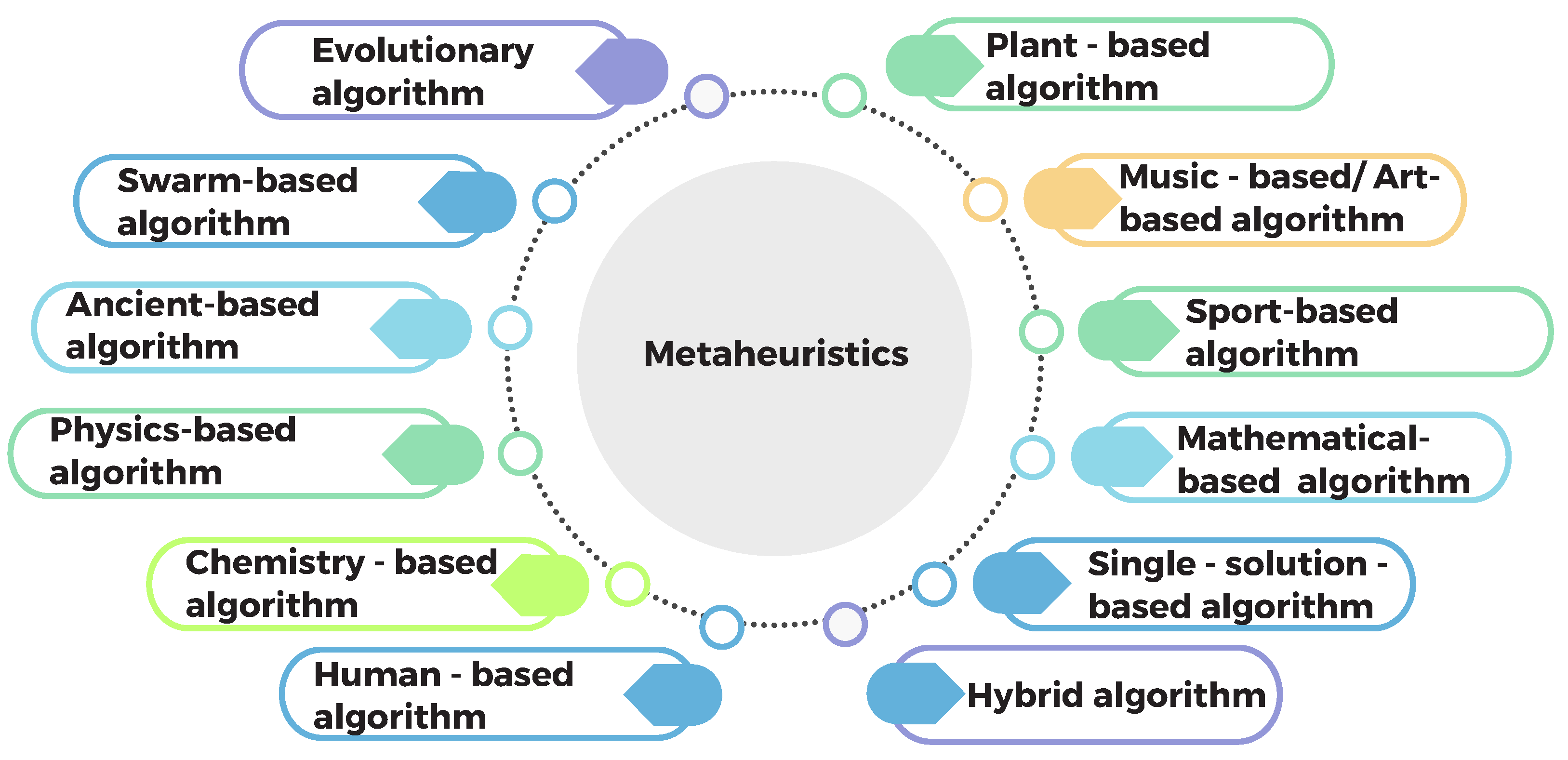
Optimization is present in several areas of engineering and applied sciences, where it is used to improve designs, reduce costs, increase efficiency, or find the best possible solution under specific constraints. Many of these real-world problems are highly complex, involving multimodal functions or nonconvex search spaces. In such cases, metaheuristics offer a powerful alternative, particularly for problems with high computational demands and intricate solution landscapes. Their main advantages include the ability to efficiently explore the search space and reduce the risk of becoming trapped in local optima. Several metaheuristic algorithms have been proposed, inspired by modeling biological behavior, chemical processes, or physical phenomena. They can be classified into twelve categories [1], as shown in Figure 1, according to their fundamental principles, as follows:
  • Evolutionary algorithms: Genetic Algorithm (GA) [2,3], Cultural Algorithm (CA) [4], Memetic Algorithm (MA) [5], Gene Expression Programming (GEP) [6], Evolutionary Strategy (ES) [7], Gradient Evolution Algorithm (GEA) [8], Differential Evolution (DE) [9], Liver Cancer Algorithm (LCA) [10], Evolutionary Mating Algorithm (EMA) [11], and Clustered-Vectors Optimization algorithm (CVO) [12].
  • Swarm-based algorithms: Particle Swarm Optimization(PSO) [13]), Golden Jackal Optimization (GJO) [14], Black Widow Optimization (BWOA) [15], Jumping Spider optimization algorithm (JSOA) [16], Horned Lizard Optimization Algorithm(HLOA) [1], Fennec Fox Algorithm (FFA) [17], Dingo Optimization Algorithm (DOA) [18], Artificial Rabbits Optimization (ARO) [19], Tunicate Swarm Algorithm (TSA) [20], Mantis Shrimp Optimization Algorithm (MShOA) [21], Harris hawks Optimization Algorithm (HHO) [22], Bonobo optimizer (BO) [23], Salp Swarm Algorithm (SSA) [24], Ant Lion Optimizer (ALO) [25], Mexican Axolotl Optimization Algorithm (MAO) [26], and Mountain Gazelle Optimizer [27].
  • Ancient-based algorithms: Giza Pyramids Construction (GPC) [28], Tianji’s horse racing optimization (THRO) [29], Al-Biruni Earth Radius (BER) Metaheuristic Search Optimization Algorithm [30], Great Wall Construction Algorithm (GWCA) [31], and Dujiangyan Irrigation System Optimization (DISO) [32].
  • Physics-based algorithms: Simulated Annealing (SA) [33], Gravitational Search Algorithm (GSA) [34], Thermal Exchange Optimization (TEO) [35], Momentum Search Algorithm (MSA) [36], Light Spectrum Optimizer (LSO) [37], Kepler optimization algorithm (KOA) [38], Artificial Satellite Search Algorithm (ASSA) [39], and Vibrating Particles System Algorithm [40].
  • Chemistry-based algorithms: Chemical Reaction Optimization (CRO) [41], Enzyme action optimization (EAO) [42], Crystal Structure Algorithm (CryStAl) [43], and Chemical Reaction Pathway Algorithm (CRPA) [44].
  • Human-based algorithms: Teamwork Optimization Algorithm (TOA) [45], Coronavirus Mask Protection Algorithm (CMPA) [46], Sewing Training-Based Optimization (STBO) [45], Stock Exchange Trading Optimization (SETO) [47], Revolution Optimization Algorithm (ROA) [48], and Osprey Optimization Algorithm (OOA) [49].
  • Plant-based algorithms: Waterwheel Plant Algorithm (WWPA) [50], Willow Catkin Optimization Algorithm (WCO) [51], and Strawberry Algorithm (SBA) [52].
  • Music-based/Art-based algorithms: Stochastic Paint Optimizer [53] and Color harmony algorithm (CHA) [54].
  • Sport-based algorithms: Puzzle Optimization Algorithm (POA) [55], Running City game optimizer (RCGO) [56], Alpine Skiing Optimization (ASO) [57], Basketball team optimization algorithm (BTOA) [58], and Golf Sport Inspired Search (GSIS) [59].
  • Mathematical-based algorithms: Arithmetic Optimization Algorithm (AOA) [60], Newton’s Downhill Optimizer (NDO) [61], and Multi-objective exponential distribution optimizer (MOEDO) [62].
  • Single-solution-based algorithms: Tabu Search (TS) [63], Single Candidate Optimizer (SCO) [64], and Variable Neighbourhood Search (VNBS) [65].
  • Hybrid algorithms: Butterfly Optimization Algorithm Combined with Black Widow Optimization (BFA-BWOA) [66], Equilibrium Whale Optimization Algorithm (EWOA) [67], Cuckoo optimization algorithm and SailFish optimizer (COA-SFO) [68], Improved Dingo Optimization Algorithm (IDOA) [69], Cuckoo Search and Stochastic Paint Optimizer (CSSPO) [70], Elite opposition-based learning, Chaotic k-best gravitational search strategy, and Grey wolf optimizer (EOCSGWO) [71], Hybrid Mutualism Mechanism-inspired Butterfly and Flower Pollination Optimization Algorithm (HMMB-FPOA) [72], and Hybrid Pelican Komodo Algorithm (HPKA) [73].
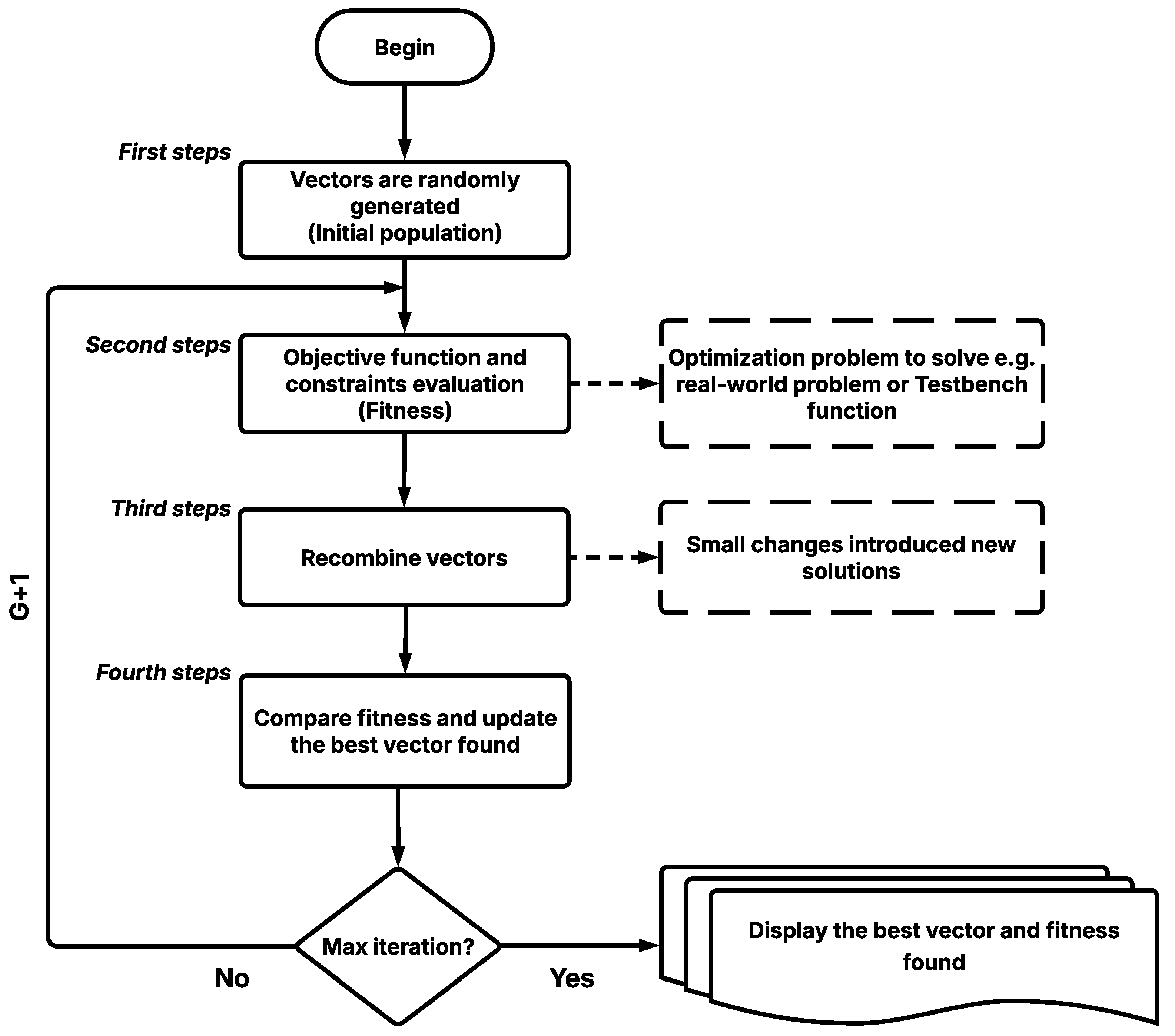
Since no unique method can universally and effectively solve all optimization problems [74], the scientific community continues to propose new algorithms to address increasingly complex optimization scenarios. A general metaheuristic algorithm framework consists of four steps, as depicted in Figure 2, and is outlined as follows:
First step: A set of possible solutions (vectors) is randomly generated. They evolve in each iteration.
Second step: The entire population is evaluated by the objective function, and the value computed is named fitness. For minimization, the goal is to find the lowest fitness.
Third step: Bio-inspired functions based on modeling biological behavior, chemical processes, or physical phenomena are used to recombine vectors.
Fourth step: The fitness of each vector, in the current iteration, is compared with the best vector in the evolutionary process. The lowest fitness is updated as the best vector.
Finally, this evolutionary process is repeated until a stop condition is met, and then the best values found are reported. Note that the number of iterations and the population size influence the algorithm’s performance in this evolutionary process. Therefore, the algorithm’s efficiency implies setting these parameters to the lowest value. Moreover, the effectiveness is related to a balance between exploitation (local search) and exploration (global search) to find feasible solutions in the search space.
The contributions of this work are the following:
  • This paper proposes the Tetragonula carbonaria Optimization Algorithm (TGCOA), a novel swarm-based metaheuristic inspired by the temperature regulation behaviors during hive construction. The TGCOA models three key strategies: slight fluttering motion to warm the hive, strong fluttering motion for hive cooling, and building the spiral hive at moderate temperatures. Note that there are no works in the literature that carry out the modeling presented.
  • The novel approach achieves a balance between local and global search through honeybee-inspired strategies: slight fluttering motion to warm the hive modeling local exploitation, while building the spiral hive at moderate temperatures simulates global exploration.
  • The TGCOA operates without additional parameters, using only a fixed population size of 30 and 200 iterations. Note that a low number of iterations contributes to the algorithm’s efficiency compared to several approaches reported in the literature that use more iterations.
  • To evaluate the efficiency and efficacy of the proposed approach, twenty benchmark functions, twenty-eight IEEE CEC 2017 constrained issues, and seven real-world engineering design challenges are used.
  • The Average Convergence Rate (ACR) metric is used to quantify the average speed at which the algorithm approaches an optimal (near-optimal) solution throughout the iterative process.
  • Statistical analysis is conducted through Wilcoxon signed-rank and Friedman tests to benchmark the TGCOA against ten bio-inspired metaheuristic algorithms taken from the literature.
  • The TGCOA’s MATLAB code is available to support this study’s findings.
The remainder of this paper’s sections are arranged as follows: Section 2 introduces the bio-inspiration behind the TGCOA, its mathematical formulation, pseudocode, and time complexity analysis. Section 3 compares the proposed approach with ten biologically inspired algorithms and evaluates its effectiveness using a variety of testbed functions by contrasting the results with Wilcoxon and Friedman statistical tests. In Section 4, the results and discussion are presented. The constraint-handling technique employed, as well as the application of the TGCOA to real-world optimization problems, are detailed in Section 5. Finally, the conclusions and recommendations for future research are summarized.

2. Tetragonula carbonaria Optimization Algorithm (TGCOA)

2.1. Biological Fundamentals

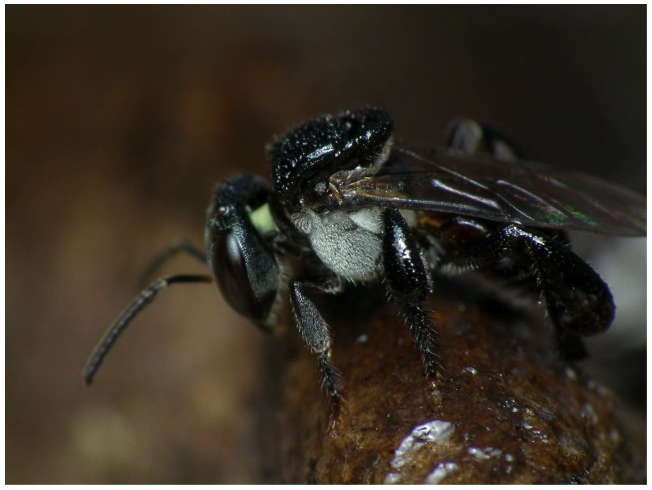
Tetragonula carbonaria, often referred to as the sugar sac bee or bush bee, is a group of eusocial insects found predominantly in Southeast Asia and Australia [75,76,77,78,79,80]. These bees are well known for their excellent honey production capacity and their ability to pollinate a wide range of crops. Tetragonula carbonaria worker bees are tiny, measuring between 3.9 and 4.3 mm in body length (see Figure 3), and they can generate approximately 2 kg of honey per year [81].
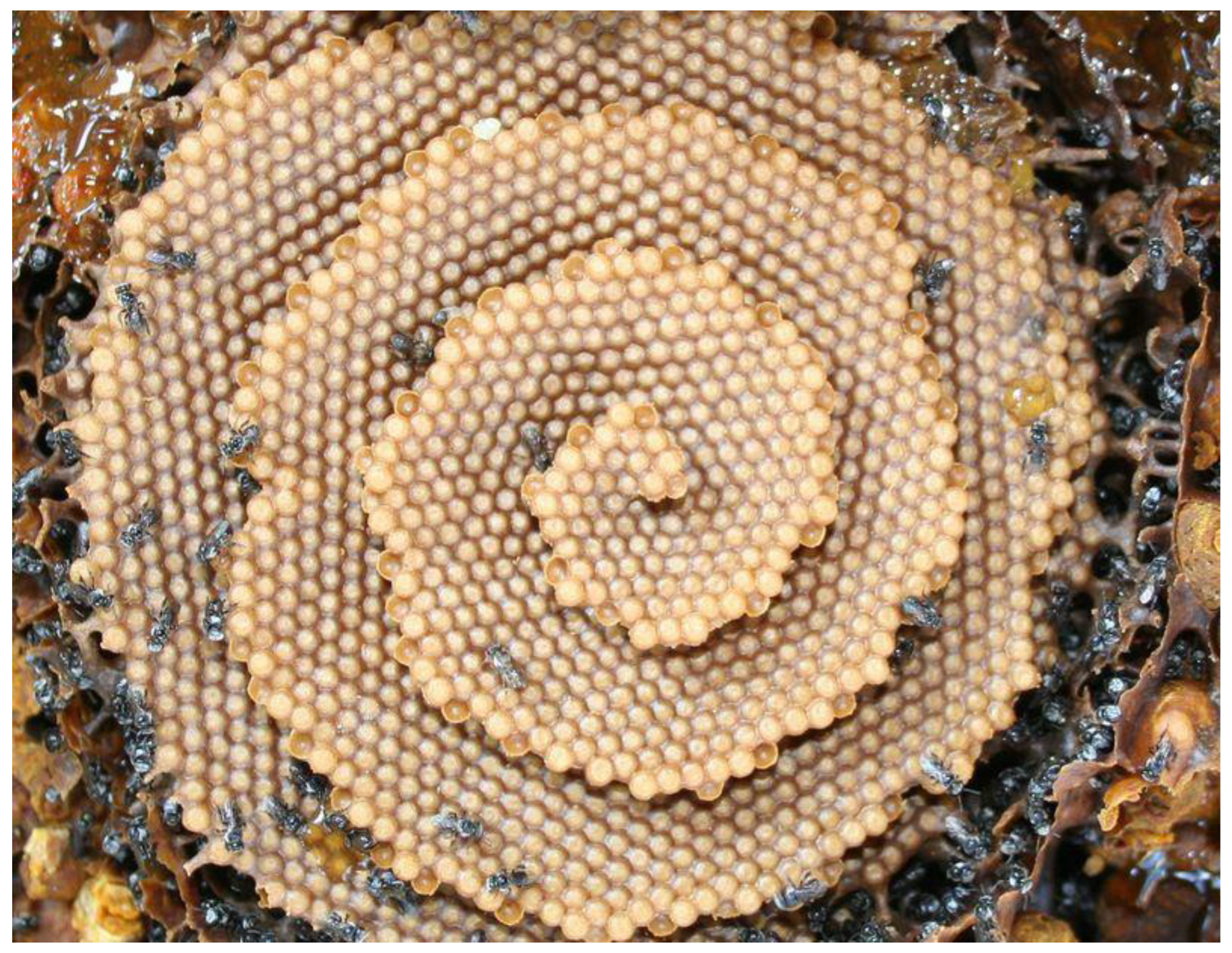
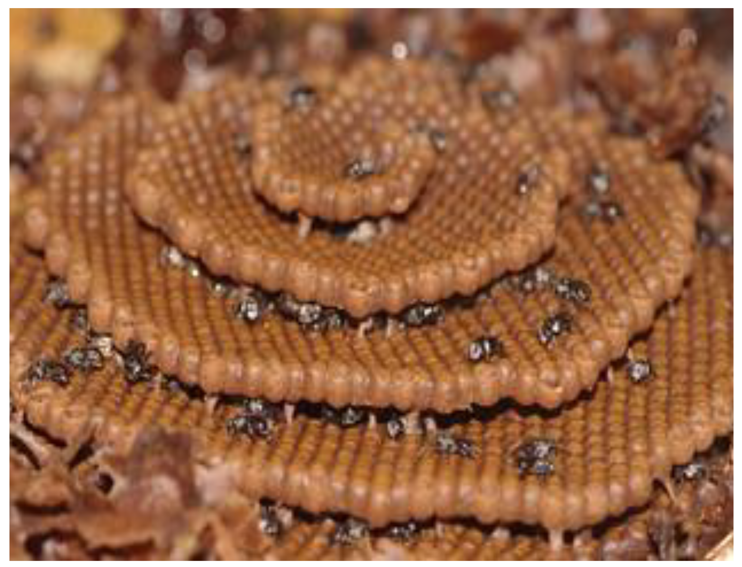
One of its outstanding characteristics is the design and construction of the hive. Tetragonula carbonaria, unlike other bees, builds a hive with a three-dimensional spiral arrangement composed of terraces placed on top of each other, as shown in Figure 4.
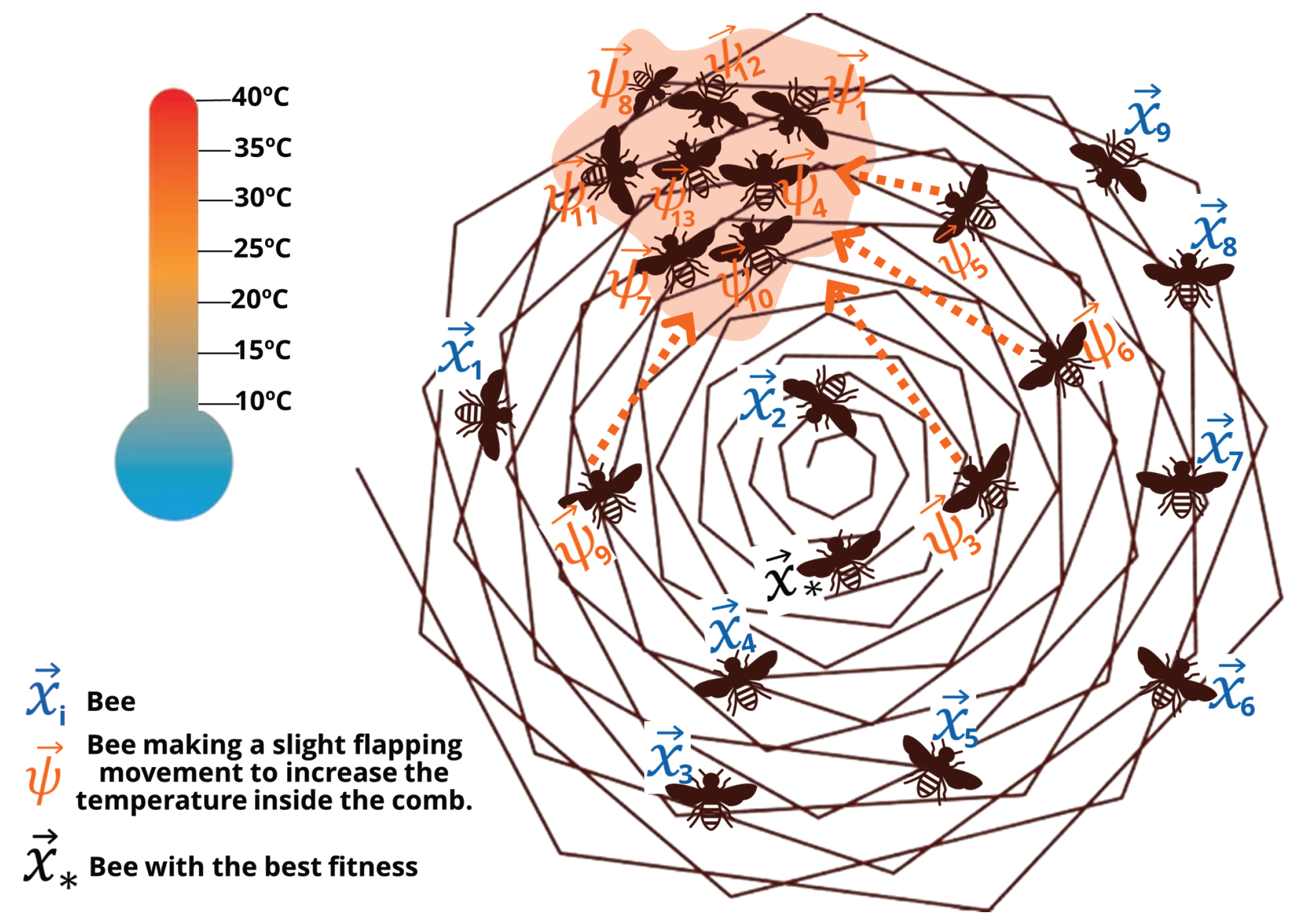
The architecture of the Tetragonula carbonaria hive is profoundly influenced by environmental temperature, which determines whether the bees prioritize heat generation, efficient expansion, or ventilation of the nest. At low temperatures, between 10 and 17 °C, some worker bees cluster together and perform a slight fluttering motion to warm the hive and safeguard the brood. Meanwhile, for high temperatures, ranging from 30 to 40 °C, the fluttering motion increases as a cooling regulation mechanism. Finally, when temperatures range between 18 and 29 °C, there is no fluttering movement, and bees focus on building the spiral comb [82,83]. The construction dynamic is staggered, where the bees build new cells at the edges, fill those cells with eggs, and seal them before moving on to the next level [84]. The hexagonal geometry of the cells allows an efficient distribution of space and favors air circulation, key for comb development [85]. Each bee collaborates indirectly within a decentralized system; the task to be performed is communicated through changes in the hive’s temperature-driven environment; this mechanism is known as stigmergy [86,87].

2.2. Mathematical Model and Optimization Algorithm

The research focuses on modeling the collective construction and thermoregulatory behavior of Tetragonula carbonaria. Inspired by the way bees work together in their hive, responding to temperature changes, a new algorithm is created that mimics how bees change their behavior based on their surroundings. The model reproduces the dynamic strategies used by the colony to conserve thermal stability and expand the spiral structure of the comb.

2.2.1. Slight Fluttering Motion and Cluster to Warm the Hive

Slight fluttering motion consists of subtle vibrations of the bees’ wings without actually flying. This mechanism activates thermogenesis at temperatures between 10 and 17 °C, causing the worker bees to cluster near the brood to generate heat and maintain a stable temperature inside the comb [88,89]. This mechanism is depicted in Figure 5, and, mathematically, based on Fourier’s Law [90], it is represented by the following equation:
Q = d T d x · A · k
where Q is the heat flux (in watts, W), d T d x represents the temperature gradient (temperature variation per unit length), A is the cross-sectional area through which heat flows, and k is the thermal conductivity of the material (in W/m·C). Equation (2) can be represented as follows:
d T d x = Δ T ( t ) = r = 1 n b ψ r ( t ) x i ( t ) n b
where ψ r ( t ) x i ( t ) represents the temperature variation. ψ r ( t ) denotes the r-th randomly generated subset of bees at generation t, which clusters to increase the hive temperature by a slight fluttering motion, ψ X , where X is the population of bees. x i ( t ) is the current i-th worker bee in the generation t. n b is a randomly generated integer that indicates the number of bees that will be clustered to warm the hive. Equation (3) can be rewritten as
x i ( t + 1 ) = 1 2 x ( t ) + Δ T ( t ) · A 2 · k
In this model, x i ( t + 1 ) represents the position of the i-th worker bee (search agent) in the solution search space at iteration t + 1 . x ( t ) represents the best search agent found in the current generation t. Δ T ( t ) represents the temperature variation shown in Equation (3). A is the flutter amplitude randomly generated between 0.2 and 0.3 mm. Finally, k represents thermal conductivity set to 0.03 W/m·C (Watts per meter-Celsius). The pseudocode for this method is presented in Algorithm 1.
Algorithm 1 Slight Fluttering Motion and Cluster of Bees
1:
  Input: Population size S i z e P o p
2:
  Output: Updated bee positions
3:
  procedure SlightFlapping
4:
     Generate a random integer n b [ 1 , S i z e P o p ]
5:
     Generate a vector of n b random integer indices r [ 1 , S i z e P o p ]
6:
     Generate the subset ψ r P o p u l a t i o n         ▹ Bees that flutter to increase temperature
7:
     Generate a random flutter amplitude A [ 0.2 , 0.3 ]
8:
     Update the bee position using Equation (4)
9:
     return Updated bee positions
10:
 end procedure

2.2.2. Strong Fluttering Motion and Clustering for Hive Cooling

The intensified fluttering movement occurs at high ambient temperatures, between 30 and 40 °C, and serves as a cooling mechanism to regulate the internal temperature of the hive [76]. This mechanism is depicted in Figure 6 and mathematically represented by the following equation:
x i ( t + 1 ) = x ( t ) 1 2 x ( t ) + Δ T ( t ) · c f ( t ) · A 2 · k
In this model, x i ( t + 1 ) represents the position of the i-th worker bee (search agent) in the solution search space at iteration t + 1 . x ( t ) represents the best search agent found in the current generation t. Δ T ( t ) represents the temperature variation shown in Equation (3). A is the flutter amplitude randomly generated between 0.2 and 0.3 mm. Finally, k represents thermal conductivity, set to 0.03 W/m·C (Watts per meter-Celsius).
c f ( t ) = ( α 1 ) t Max iter α α
c f ( t ) is a cooling factor that dynamically modulates the step size as the algorithm progresses.   α represents the number of wing flutterings per second performed by a bee, set to 50. M a x iter represents the maximum number of iterations. The pseudocode of this strategy is shown in Algorithm 2.
Algorithm 2 Strong Fluttering Motion and Cluster of Bees
1:
 Input: Population size S i z e P o p
2:
 Output: Updated bee positions
3:
 procedure  StrongFlapping
4:
    Generate a random integer n b [ 1 , S i z e P o p ]
5:
    Generate a vector of n b random integer indices r [ 1 , S i z e P o p ]
6:
    Generate the subset ψ r P o p u l a t i o n         ▹ Bees that flutter to dissipate heat
7:
    Generate a random flutter amplitude A [ 0.2 , 0.3 ]
8:
    Update the bee position using Equation (5)
9:
    return Updated bee positions
10:
end procedure

2.2.3. Building the Spiral Hive

Bees focus on optimizing comb construction when the temperature ranges between 18 °C and 29 °C, thereby minimizing their metabolic and thermoregulatory demands [91,92,93]. In these favorable thermal conditions, bees build a geometric spiral pattern through stigmergy. The movement of the bee to build the next cell is mathematically represented as follows:
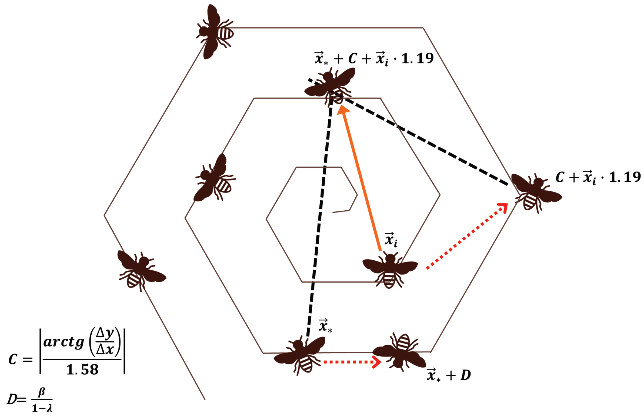
x i ( t + 1 ) = x ( t ) + β 1 λ
where x i ( t + 1 ) represents the position of the i-th worker bee (search agent) in the solution search space at iteration t + 1 . x ( t ) represents the best search agent found in the current generation t. β is a random uniform distribution value in the range ( 0 , 1 ) , introducing slight variation in the movement. λ is a random number generated from a standard Cauchy distribution with median set to 0 and the scale parameter set to 1. This model simulates the bees’ short-range displacements around their position, enabling them to perform local searches and fine-tune the placement of new comb cells for construction.
Hive spiral geometry is based on the Archimedean spiral and is represented using polar angles in the polar coordinate system, as shown in the following equation:
Δ x = a + b · θ · cos ( θ ) , Δ y = a + b · θ · sin ( θ ) ,
Thereby, Equation (8) can be re-defined as follows:
x i ( t + 1 ) = x ( t ) + arctg Δ y Δ x 1.58 · x i ( t ) · 1.19
In this model, x i ( t + 1 ) represents the position of the i-th worker bee (search agent) in the solution search space at iteration t + 1 . x ( t ) represents the best search agent found in the current generation ta represents the distance from the origin to the starting point of the spiral, set to 0, and b defines how far the spiral expands from the origin for each unit of angular increase, set to 10. The value 1.58 corresponds to a normalization factor that regulates the influence of the spiral angle.   x i ( t ) is the current i-th worker bee in the generation t. The average distance between cells in the comb structure is reflected by the adjustment coefficient, which stands at 1.19 mm.
The angular parameter θ controls the spiral tightening and is computed as follows:
θ = 90 90 · t Max iter · π 180
where t denotes the current iteration, Max iter is the maximum number of iterations, and   π 180 converts the angle from degrees to radians.
Note that the hive construction phase is based on Equations (7) and (10), which are randomly selected as shown in Algorithm 3. Equation (7) represents the construction of cell around the bee, while Equation (10) corresponds to the spiral construction. The whole strategy of building the spiral hive is depicted in Figure 7. Additionally, the pseudocode is presented in Algorithm 3.
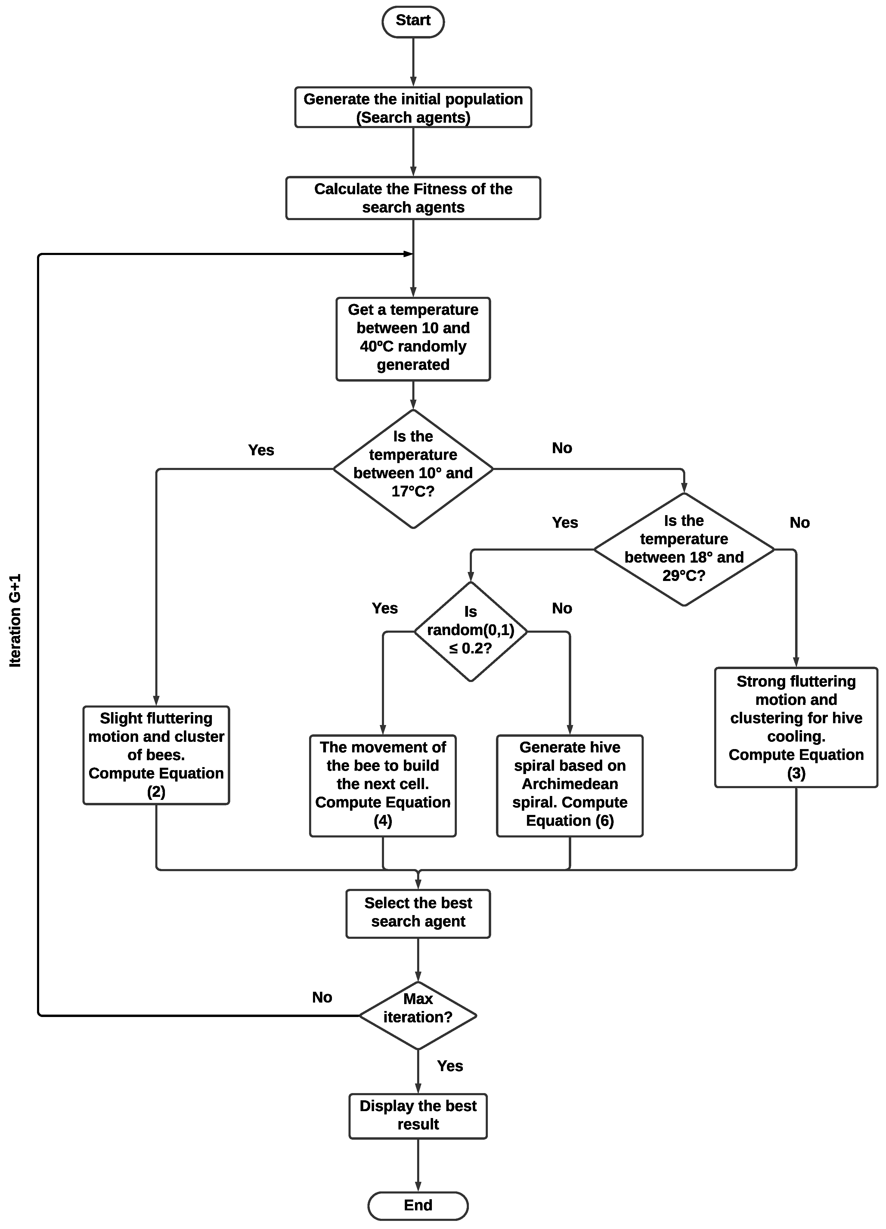
All strategies are summarized in a flowchart, as shown in Figure 8, as well as in Algorithm 4.
Algorithm 3 Building the Spiral Hive
1:
  Input: Current population of bees
2:
  Output: Updated bee positions
3:
  procedure  SpiralHive
4:
    Identify the best solution vector x ( t ) from the current population
5:
    Generate a random value β ( 0 , 1 ) from a uniform distribution
6:
    Generate λ Cauchy ( 0 , 1 )
7:
    if  r a n d 0.2  then
8:
        Construct the cell around the bee using Equation (7)
9:
    else
10:
        Construct hive spiral based on Archimedean spiral using Equation (9)
11:
    end if
12:
    return Updated bee positions
13:
end procedure

2.3. Pseudocode for TGCOA

Algorithm 4 outlines the pseudocode for the TGCOA.
Algorithm 4Tetragonula carbonaria Optimization Algorithm (TGCOA)
1:
  Input: Search agents, maximum number of iterations, population size
2:
  Output: Best solution x
3:
  procedure  TGCOA
4:
    Initialize parameters: define search agents, max iterations, and population size
5:
    Generate the initial population randomly
6:
    while iteration < MaxIterations do
7:
        Generate a random temperature in the range [10, 40] °C
8:
        if Temperature between 10 °C and 17 °C then
9:
           Slight fluttering motion and cluster of bees Equation (4)
10:
      else if Temperature between 18 °C and 29 °C then         ▹ Building the spiral hive
11:
         if random 0.2  then
12:
             Construct the cell around the bee Equation (7)
13:
         else
14:
             Construct hive spiral based on Archimedean spiral Equation (9)
15:
         end if
16:
      else
17:
         Strong fluttering motion and clustering for hive cooling Eq.5
18:
      end if
19:
      Calculate x new , the fitness value of the new search agents
20:
      if  x new < x  then
21:
          x x new
22:
      end if
23:
      iteration ← iteration + 1
24:
  end while
25:
  Display x , the best optimal solution
26:
end procedure

2.4. The TGCOA’s Time Complexity

Computational complexity is defined by a function that correlates the execution time of the method with the magnitude of the problem input, and Big-O notation is used to represent it. The time complexity of the TGCOA depends on the number of iterations ( M a x I t e r a t i o n ), the population size of bees (nBee), the problem’s dimensionality (D), and the cost of the objective function f. Based on the pseudocode shown in Algorithm 4, a detailed analysis is presented in Table 1.
The overall time complexity of the TGCOA can be computed as follows:
O ( TGCOA ) = O ( n B e e . D ) + O ( 1 ) + O ( n B e e . D ) + O ( n B e e . f ) + O ( 1 ) + O ( M a x I t e r a t i o n n B e e ( D + f ) ) + O ( 1 )
In O notation, when we add several terms, the fastest-growing one dominates. Hence, the time complexity of the TGCOA can be expressed as follows:
O ( TGCOA ) = O ( M a x I t e r a t i o n n B e e ( D + f ) )

3. Experimental Setup

To evaluate the effectiveness and stability of the proposed TGCOA in solving numerical optimization problems, a set of 20 well-known test functions was used. The set has 10 unimodal functions and 10 multimodal functions. Single-mode functions are associated with local searches (exploitation), whereas multimodal functions relate to global searches (exploration) in the solution search space. Appendix A provides an overview of these functions. Their classification is presented in Table A1, and their description is shown in Table A2, where D i m indicates the dimension, I n t e r v a l is the boundary of the search space, and f m i n is the best-known optimal value. The TGCOA algorithm was compared against ten bio-inspired algorithms taken from the literature, which are described as follows:
  • Black Widow Optimization Algorithm (BWOA): The algorithm, inspired by Latrodectus spider reproductive strategies, balances exploration and exploitation through natural phenomena like mate selection, pheromone rate, and cannibalism after mating [15].
  • Jumping Spider Optimization Algorithm (JSOA): This algorithm resembles the natural behavior of Salticidade spiders, mathematically modeling their hunting strategies, such as searching, jumping, and pursuing [16].
  • Liver Cancer Algorithm (LCA): It is based on tumor growth dynamics, consisting of three stages: tumor clonal expansion, vascular recruitment, and metastatic leap, using adaptive mutation, neighborhood sampling, and opposition-based learning [10].
  • Evolutionary Mating Algorithm (EMA): The Hardy–Weinberg equilibrium, a fundamental concept in population genetics, is the basis for modeling genetic diversity and selection in natural populations [11].
  • Bonobo Optimizer (BO): The algorithm, inspired by the social and reproductive strategies of bonobos, balances exploration and exploitation through behaviors such as fission–fusion grouping, diverse mating patterns, and selective mate interaction [23].
  • Salp Swarm Algorithm (SSA): Based on the swarming dynamics of salps in marine ecosystems, this algorithm mimics their coordinated movement during navigation and foraging [24].
  • Ant Lion Optimizer (ALO): The algorithm simulates the hunting strategy of antlions by modeling five key stages: random wandering, trap construction, prey capture, and subsequent trap rebuilding [25].
  • Mexican Axolotl Optimization Algorithm (MAO): The algorithm mimics the life cycle and adaptive traits of axolotls; the algorithm emulates key processes such as regenerative healing, reproductive strategies, and tissue restoration [26].
  • Particle Swarm Optimization (PSO): Inspired by the collective behavior of flocks of birds and schools of fish, optimizing through the collaborative movement of particles in the search space, balancing exploration and exploitation [13].
  • Differential Evolution (DE): The algorithm optimizes solutions through mutation, crossover, and selection, combining weighted differences between vectors in the population and replacing the worst with the best in each generation [9].
Each algorithm’s testbench function was independently executed 30 times, with a population size and number of iterations of 30 and 200, respectively. Moreover, the Wilcoxon signed-rank test was used to compare statistically significant differences in performance, while the Friedman test was used to rank all algorithms. It is important to highlight that a non-parametric Wilcoxon signed-rank test was performed to compare two related algorithms, with a significance level of 5%. The null hypothesis assumes no significant difference between the paired algorithms, while the alternative hypothesis suggests a difference; a p-value less than 0.05 leads to rejection of the null hypothesis. Additionally, the Friedman test was applied to rank all algorithms within each test instance. Note that a lower value indicates better performance and a higher ranking position.
The four algorithms with the highest ranks were then selected for additional evaluation on the IEEE CEC 2017 “Constrained Real-Parameter Optimization” benchmark suite [94]. This set includes 28 constrained optimization functions and was tested for dimensions of 10, 30, 50, and 100. The description of the functions is provided in Appendix A in Table A3. Additionally, seven constrained real-world design engineering problems were solved.
The parameter configurations corresponding to each optimization method are detailed in Table 2. All experiments were computed on a desktop with the following specifications: Intel Core i9-13900K processor @ 5.8 GHz, 192 GB RAM, MATLAB R2024a compiler, and Linux Ubuntu 24.04 LTS operating system.

Average Convergence Rate Analysis

The Average Convergence Rate (ACR) is a quantitative metric used to evaluate the average rate at which an optimization algorithm approaches the optimal solution during its iterative process [95,96]. It measures convergence speed in a normalized manner, making it suitable for comparing different algorithms and configurations. The ACR for a single run is defined as
ACR = 1 T 1 t = 1 T 1 f t + 1 f t f 0 f ,
where T is the total number of iterations. The numerator f t + 1 f t represents the improvement between consecutive iterations. The denominator f 0 f normalizes the improvement relative to the total possible improvement in that run. f t denotes the best objective function value obtained at iteration t, f 0 the initial value, and f the best value found during the entire optimization process. Moreover, for R independent runs, the average ACR is given by the following equation:
ACR ¯ = 1 R r = 1 R ACR r ,
where ACR r denotes the convergence rate for run r. A rapid convergence toward the optimum (near optimum) occurs when ACR 1 . Meanwhile, stagnation occurs for ACR 0 . A complete interpretation of the ACR value is shown in Table 3. This metric was used for each algorithm’s testbench function. It was independently executed 30 times, with a population size of 30 and a number of iterations of 200.

4. Results and Discussion

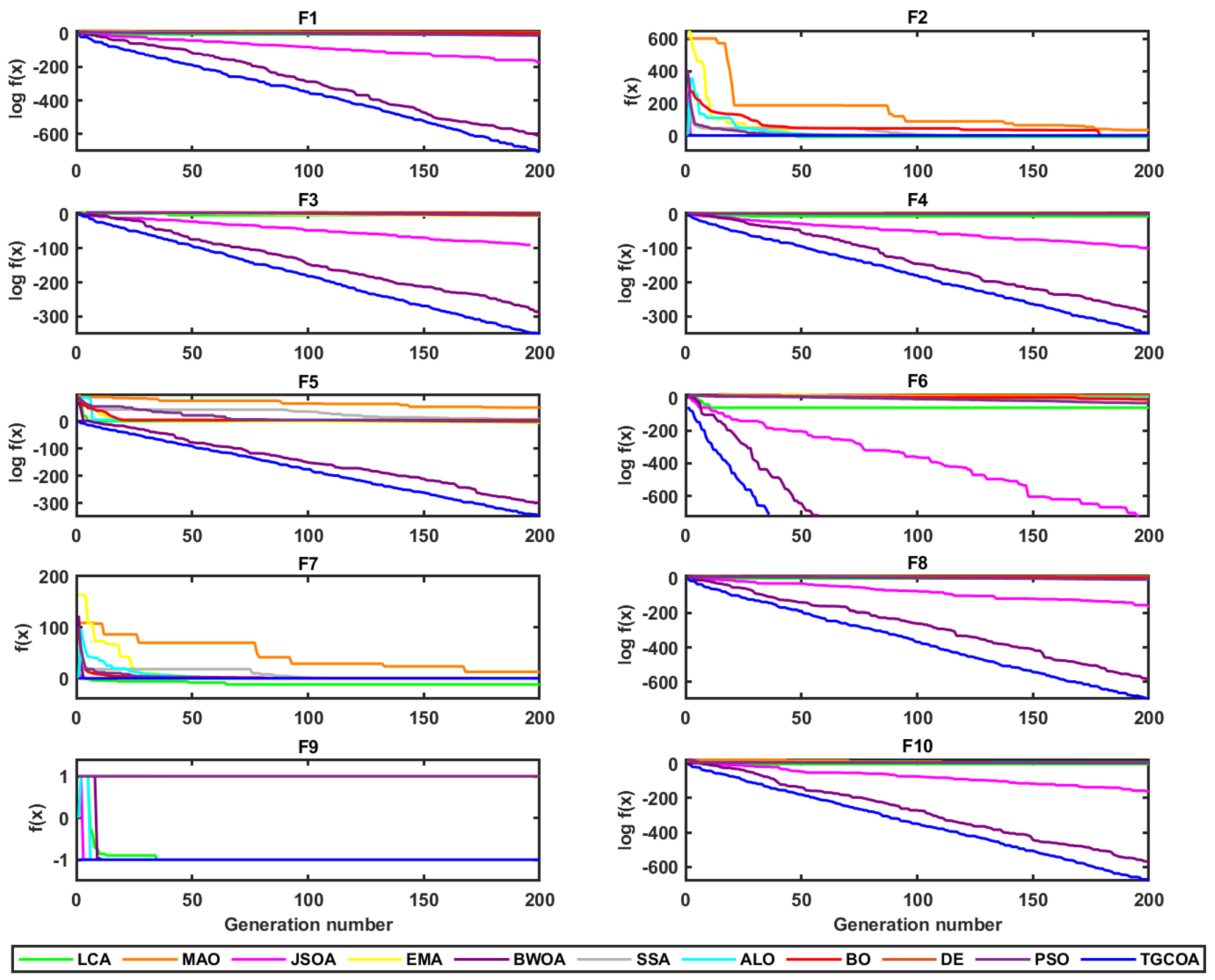
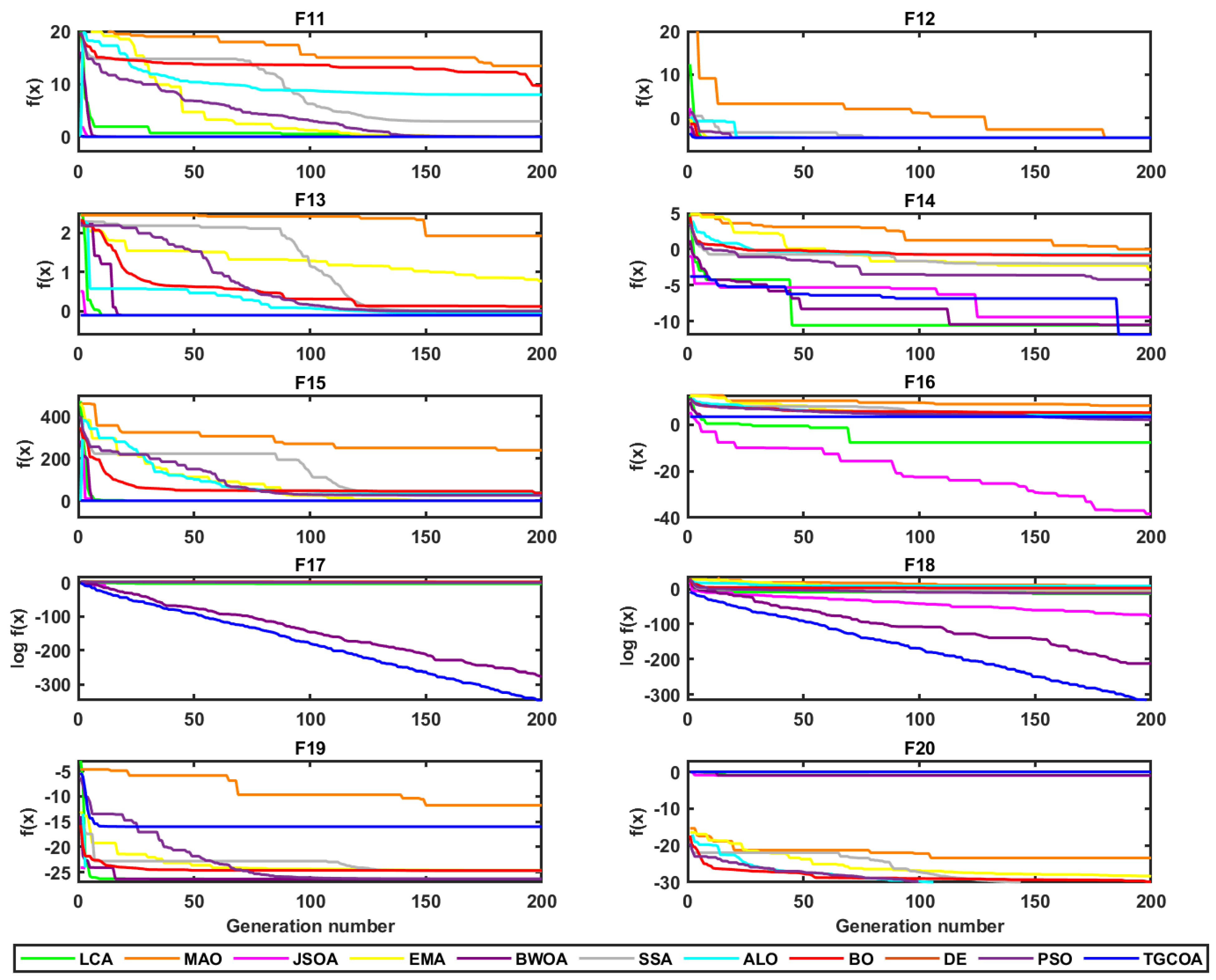
This section presents the computational outcomes of the TGCOA on testbench optimization problems. Table 4, Table 5, Table 6 and Table 7 present the comparative findings, including the optimal, average, and standard deviation values. Furthermore, Figure 9 and Figure 10 summarize the convergence graphs of all the functions compared to the other selected methods for this study. To evaluate the significant differences observed between the TGCOA and the other methods, a non-parametric statistical test, the Wilcoxon signed-rank test, was performed, establishing a significance level of 5%. The null hypothesis indicates that there is no significant difference between the two pairs of algorithms compared. Meanwhile, the alternative hypothesis suggests that there is. It is worth noting that, with a p-value less than 0.05, the null hypothesis is rejected. The results of the Wilcoxon rank-sum test, in Table 8, demonstrate that the TGCOA outperformed the following algorithms: the Evolutionary Mating Algorithm (EMA) had a p-value of 0.001 , Liver Cancer Algorithm (LCA) 0.009 , Bonobo Optimizer (BO) 0, Salp Swarm Algorithm (SSA) 0, Ant Lion Optimizer (ALO) 0, Mexican Axolotl Optimization Algorithm (MAO) 0, Particle Swarm Optimization (PSO) 0, and Differential Evolution (DE) 0. Meanwhile, no statistically significant differences were found when compared to the Black Widow Optimization Algorithm (BWOA) and Jumping Spider Optimization Algorithm (JSOA), with p-values of 0.116 and 0.363 , respectively. Moreover, the eleven algorithms were ranked by calculating the Friedman test for 20 testbench functions. Note that a lower value indicates better performance and a higher ranking position. The results of the algorithm rankings are shown in Table 9; observe that the TGCOA is ranked first, with a mean rank 2.45, whereas the JSOA, BWOA, and LCA are ranked second, third, and fourth, with mean ranks of 2.47, 2.71, and 4.68, respectively. Based on these results, for the remainder of the paper, these four best-ranked algorithms are only used in IEEE CEC 2017 ”Constrained Real Parameter Optimization” and real-world applications.
The results derived from the computational study of the TGCOA on benchmark functions from the IEEE CEC 2017 “Constrained Real-Parameter Optimization” problems for dimensions 10, 30, 50, and 100 are presented in Table 10, Table 11, Table 12, and Table 13, respectively. These tables exhibit the maximum, average, and standard deviation calculated. A Wilcoxon signed-rank test was employed to analyze the differences among the algorithms at a significance level of 5%. Moreover, the Friedman test established the ranking of the TGCOA, BWOA, JSOA, and LCA. For 10-dimensional problems, the Wilcoxon rank-sum test in Table 14 shows that the TGCOA outperformed the BWOA and LCA, with p-values of 0 for both. Meanwhile, there are no significant differences, with the JSOA having a p-value 0.97 . In Table 15, the Friedman test ranked the TGCOA third. For 30-dimensional problems, the Wilcoxon rank-sum test in Table 16 shows that the TGCOA outperformed the LCA, with a p-value of 0.003. However, there were no significant differences for BWOA and JSOA, with p-values of 0.112 and 0.096, respectively. In addition, the Friedman test ranked the TGCOA first, as shown in Table 17. The results in Table 18 indicate that, for 50-dimensional problems, the TGCOA outperformed the BWOA and LCA, with p-values of 0.032, and 0.002. Meanwhile, no significant differences were observed for JSOA, with a p-value of 0.061. According to Table 19, the Friedman test ranked the TGCOA first. Finally, for 100-dimensional problems, the Wilcoxon rank-sum test in Table 20 shows that the TGCOA outperformed all the algorithms, BWOA, LCA, and BO, with p-values of 0.021, 0.043, and 0.003, respectively. Furthermore, the Friedman test ranked the TGCOA first, as shown in Table 21.

Average Convergence Rate Results

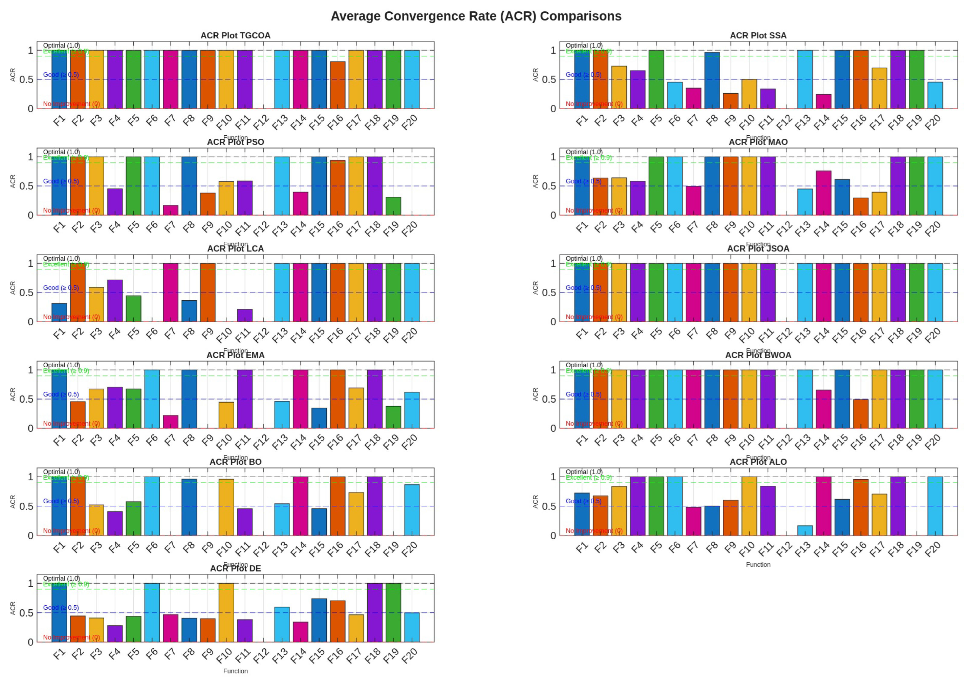
This section presents the results of the Average Convergence Rate (ACR) analysis. In Appendix A, Table A4,Table A5,Table A6,Table A7,Table A8,Table A9,Table A10,Table A11,Table A12,Table A13,A14 summarize the results obtained for the eleven algorithms on the 20 testbench functions, and the corresponding ACR plots are shown in Figure A1. Additionally, Table 22 reveals the ACR mean values computed for all the algorithms. It is important to note that the TGCOA has an ACR value greater than or equal to 0.9, which qualifies it as excellent in terms of its ability to approach the optimal (near-optimal) solution during its iterative process.

5. Real-World Applications

The capability of the TGCOA to solve real-world problems with constraints was evaluated by solving seven problems, which are as follows: tension/compression spring design, pressure vessel design, three-bar truss design problem, design of gear train, tubular column design, welded beam design, and reinforced concrete beam design, taken from [97]. For all the engineering problems solved, the TGCOA was evaluated against the top three algorithms ranked according to the Friedman test; see Table 9.
Preparatory work for implementing the TGCOA to solve other engineering optimization problems is shown in Appendix A, Table A15.

5.1. Constraint Handling

The TGCOA algorithm uses a penalty-based constraint handling technique, where infeasible solutions are penalized in their fitness value proportional to their average constraint violation. This directs the search toward feasible areas of the solution space during optimization. The mathematical formulation of this technique is described in Equation (15) and taken from [1].
F ( x ) = f ( x ) , i f M C V ( x ) 0 f max + M C V ( x ) , o t h e r w i s e .
where f ( x ) is the value of the fitness function for a feasible solution, whereas f m a x is the fitness function value of the worst solution in the population, and M C V ( x ) is the Mean Constraint Violation [1,21] represented in Equation (16).
M C V ( x ) = i = 1 p G i ( x ) + j = 1 m H j ( x ) p + m
where G i ( x ) and H j ( x ) are the inequality and equality constraints, depicted by Equations (17) and (18), respectively. Note that these functions incur a penalty when they violate the constraints.
G i ( x ) = 0 , i f g i ( x ) 0 g i ( x ) , o t h e r w i s e .
H j ( x ) = 0 , i f | h j ( x ) | δ 0 | h j ( x ) | , o t h e r w i s e
It is important to mention that no penalty coefficient is used. Instead, the Mean Constraint Violation (MCV) method is applied, where, if a solution violates a constraint, its objective function is penalized based on the fitness value of the worst solution ( f m a x ) in the population, as shown in Equations (15) and (16).

5.2. Tension/Compression Spring Design

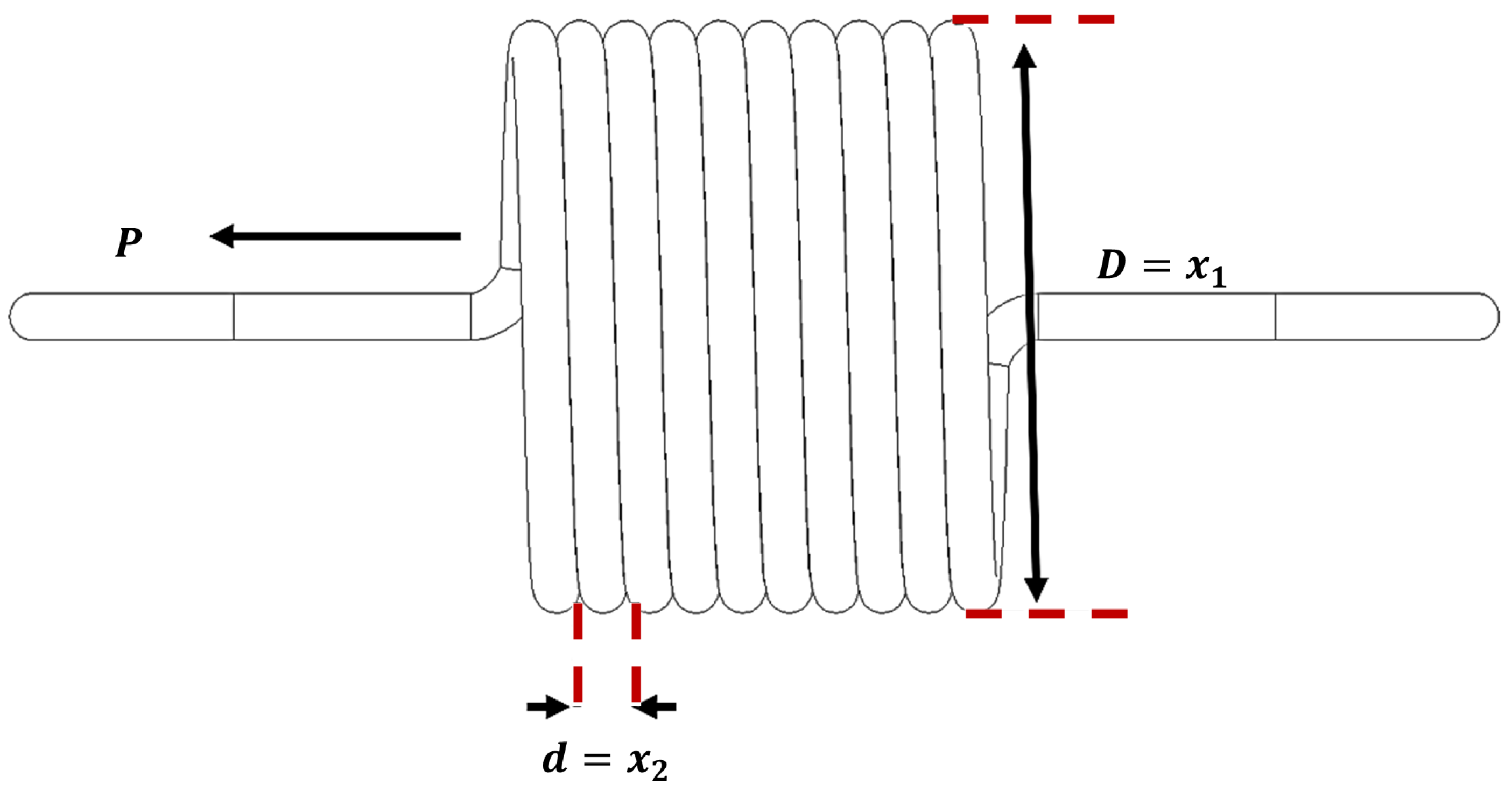
The tension/compression spring design problem, as described in [97,98] and illustrated in Figure 11, focuses on minimizing the weight of a spring under several constraints, including limits on deflection, shear stress, surge frequency, and outer diameter, as well as bounds on the design variables. These variables are the average coil diameter D = x 1 , the wire diameter d = x 2 , and the number of active coils N = x 3 . The mathematical formulation is given below:
Minimize : f ( X ) = x 3 + 2 x 2 x 1 2 Subject to g 1 ( X ) = 1 x 2 3 x 3 71785 x 1 4 0 g 2 ( X ) = 4 x 2 2 x 1 x 2 12566 x 2 x 1 3 x 1 4 + 1 5108 x 1 2 1 0 g 3 ( X ) = 1 140.45 x 1 x 2 2 x 3 0 g 4 ( X ) = x 1 + x 2 1.5 1 0 Variable range : 0.05 x 1 2 0.25 x 2 1.3 2 x 3 15
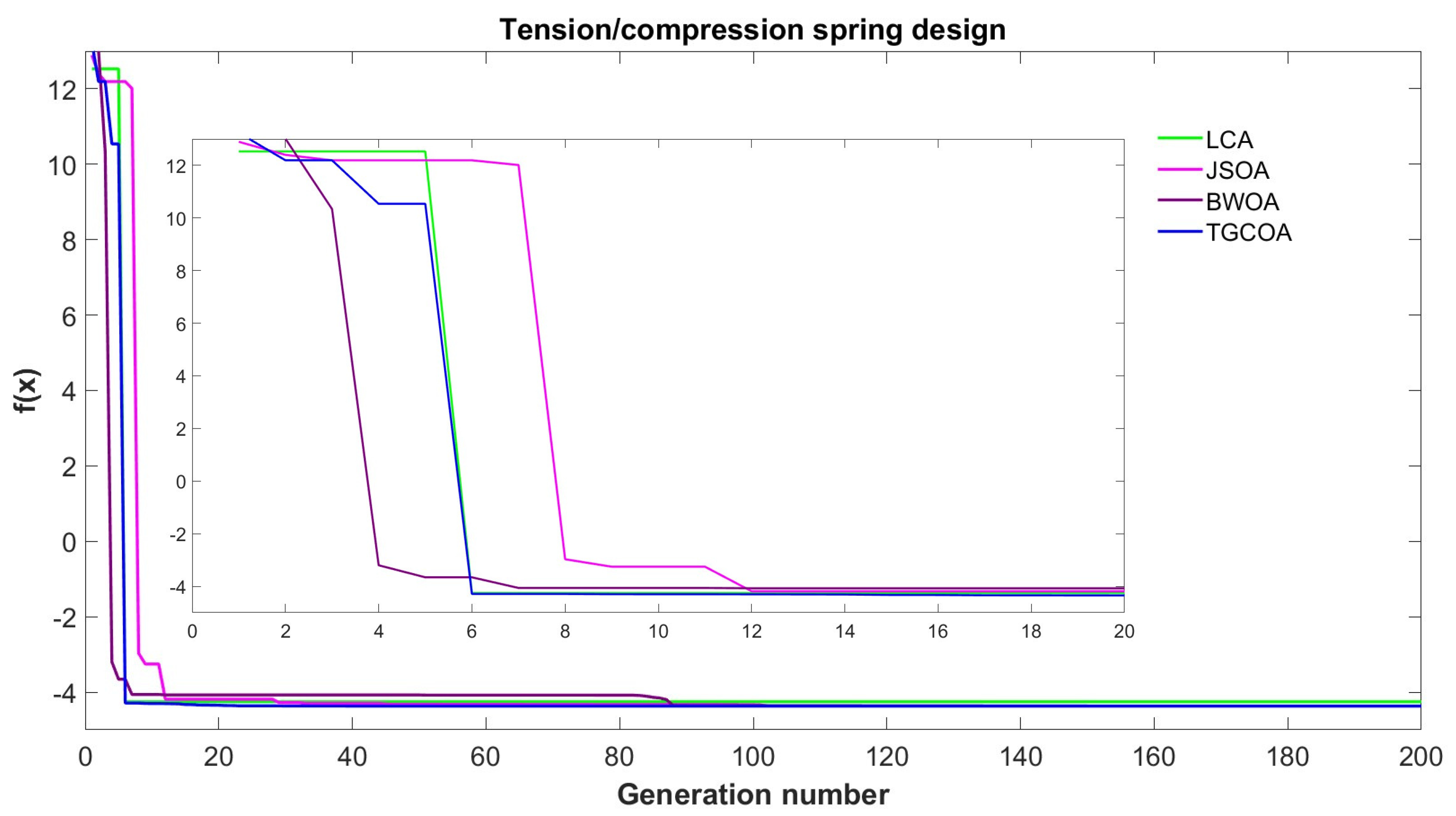
The statistical results of this test, presented in Table 23, show that all algorithms reported feasible solutions, highlighting that the TGCOA outperforms the algorithms with which it was compared, obtaining a value of 0.012665. The convergence graph is shown in Figure 12.

5.3. Pressure Vessel Design

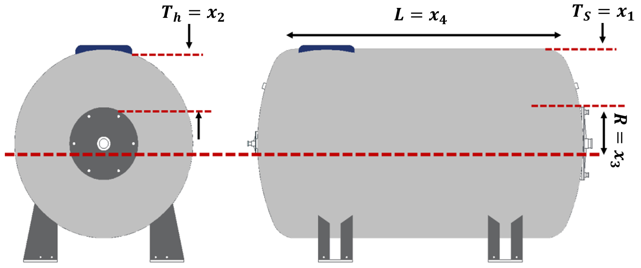
The optimization problem addresses a cylindrical pressure vessel with hemispherical caps at both ends, as shown in Figure 13. The goal is to minimize the total manufacturing cost, considering material, forming, and welding expenses. The design depends on four decision variables: x 1 , the thickness of the cylindrical body ( T 3 ); x 2 , the thickness of the hemispherical caps ( T h ); x 3 , the inner radius (R); and x 4 , the length of the cylindrical section excluding the caps (L) [97]. The variables x 1 and x 2 must be integer multiples of 0.0625 inches, while x 3 and x 4 are continuous.
Minimize : f ( X ) = 0.6224 x 1 x 3 x 4 + 1.7781 x 2 x 3 2 + 3.1661 x 1 2 x 4 + 19.84 x 1 2 x 3 , Subject to g 1 ( X ) = x 1 + 0.0193 x 3 0 g 2 ( X ) = x 2 + 0.00954 x 3 0 g 3 ( X ) = π x 3 2 x 4 4 3 π x 3 3 + 1 , 296 , 000 0 g 4 ( X ) = x 4 240 0 Variable range : x 1 , x 2 { n × 0.0625 n = 1 , 2 , , 1600 } x 3 10 , x 4 200 .
As shown in Table 24, all algorithms reported feasible solutions. Note that the TGCOA outperforms the algorithms with which it was compared, obtaining a value of 6065.4263 when minimizing the objective function. Figure 14 displays the corresponding convergence graph.

5.4. Three-Bar Truss Design Problem

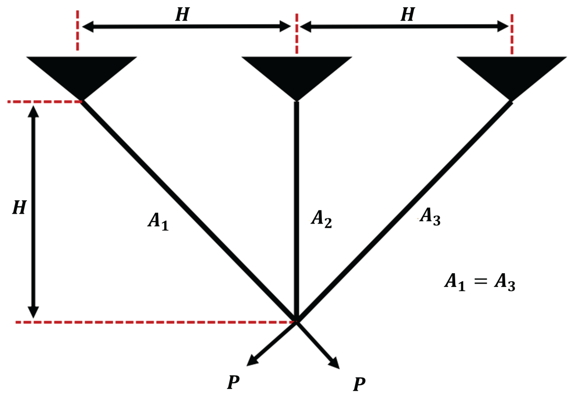
The objective is to minimize the total volume of the structure subjected to static loads while respecting the stress constraints ( σ ) in each of its elements; see Figure 15. The design variables are the cross-sectional areas A 1 = x 1 and A 2 = x 2 , whose optimum configuration is sought by means of the corresponding mathematical formulation [97].
Minimize : f ( X ) = 2 2 x 1 + x 2 · l , Subject to g 1 ( X ) = 2 x 1 + x 2 2 x 1 2 + 2 x 1 x 2 · P σ 0 , g 2 ( X ) = x 2 2 x 1 2 + 2 x 1 x 2 · P σ 0 , g 3 ( X ) = 1 2 x 2 + x 1 · P σ 0 , l = 100 cm , P = 2 kN / cm 3 , σ = 2 kN / cm 3 , Variable range : 0 x 1 , x 2 1 .
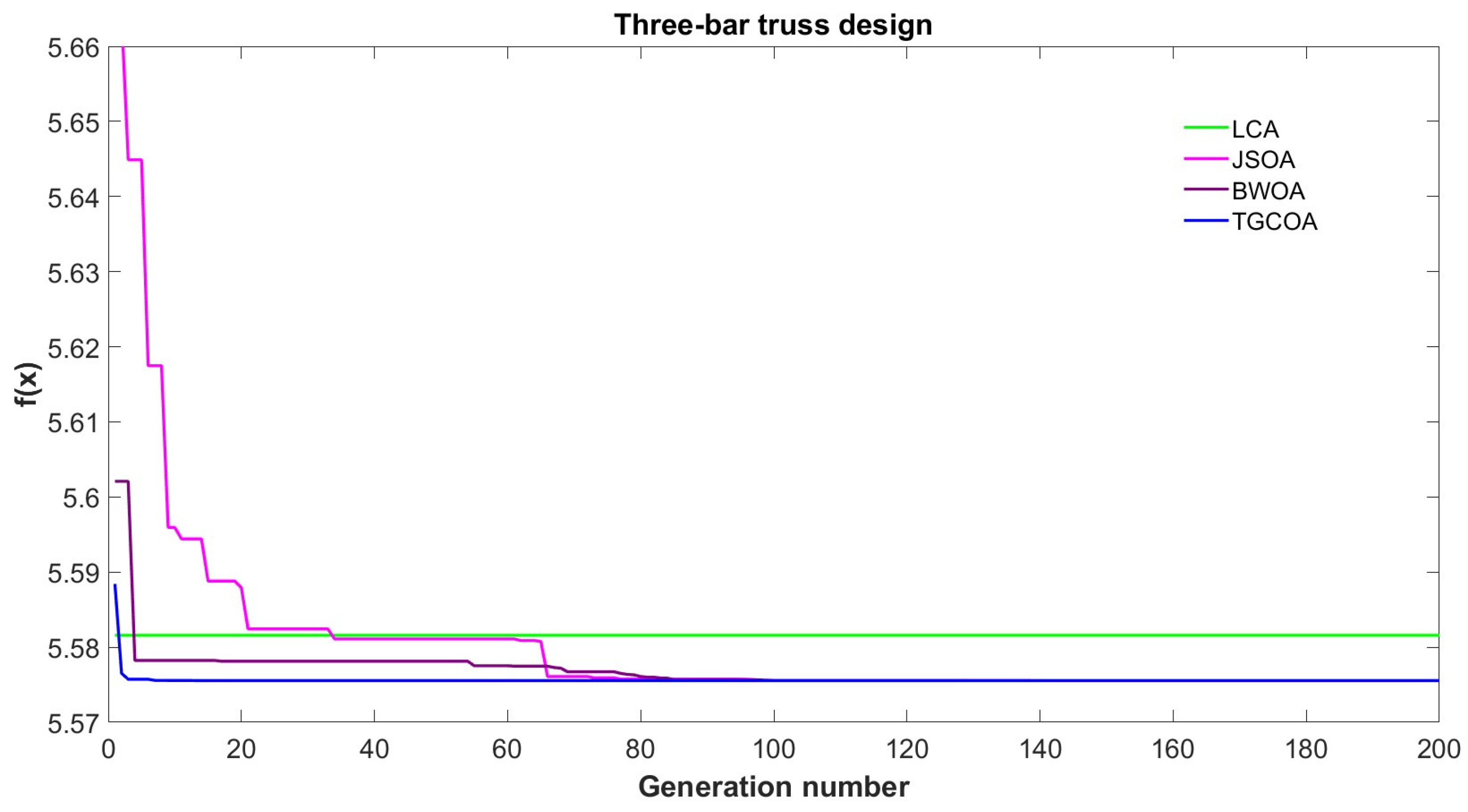
Table 25 compares the TGCOA, BWOA, JSOA, and LCA, showing that all algorithms reported feasible solutions. The TGCOA demonstrated competitive performance to BWOA and JSOA. Meanwhile, it outperformed LCA by achieving a value of 263.8958. The convergence graph is shown in Figure 16.

5.5. Design of Gear Train

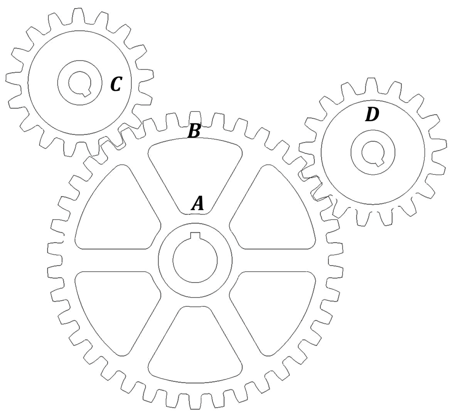
The gear train design problem taken from [97,99] is a classic case of discrete optimization in mechanical engineering. The objective is to minimize the gear ratio, defined as the ratio of the angular velocity of the output shaft to that of the input shaft. The design variables are the numbers of gear teeth n A = x 1 , n B = x 2 , n C = x 3 , and n D = x 4 . Figure 17 shows the two-dimensional model associated with this problem. The mathematical formulation is presented below.
Minimize : f ( X ) = 1 6.931 x 3 x 2 x 1 x 4 2 , Variable range : x 1 , x 2 , x 3 , x 4 { 12 , 13 , 14 , , 60 } .
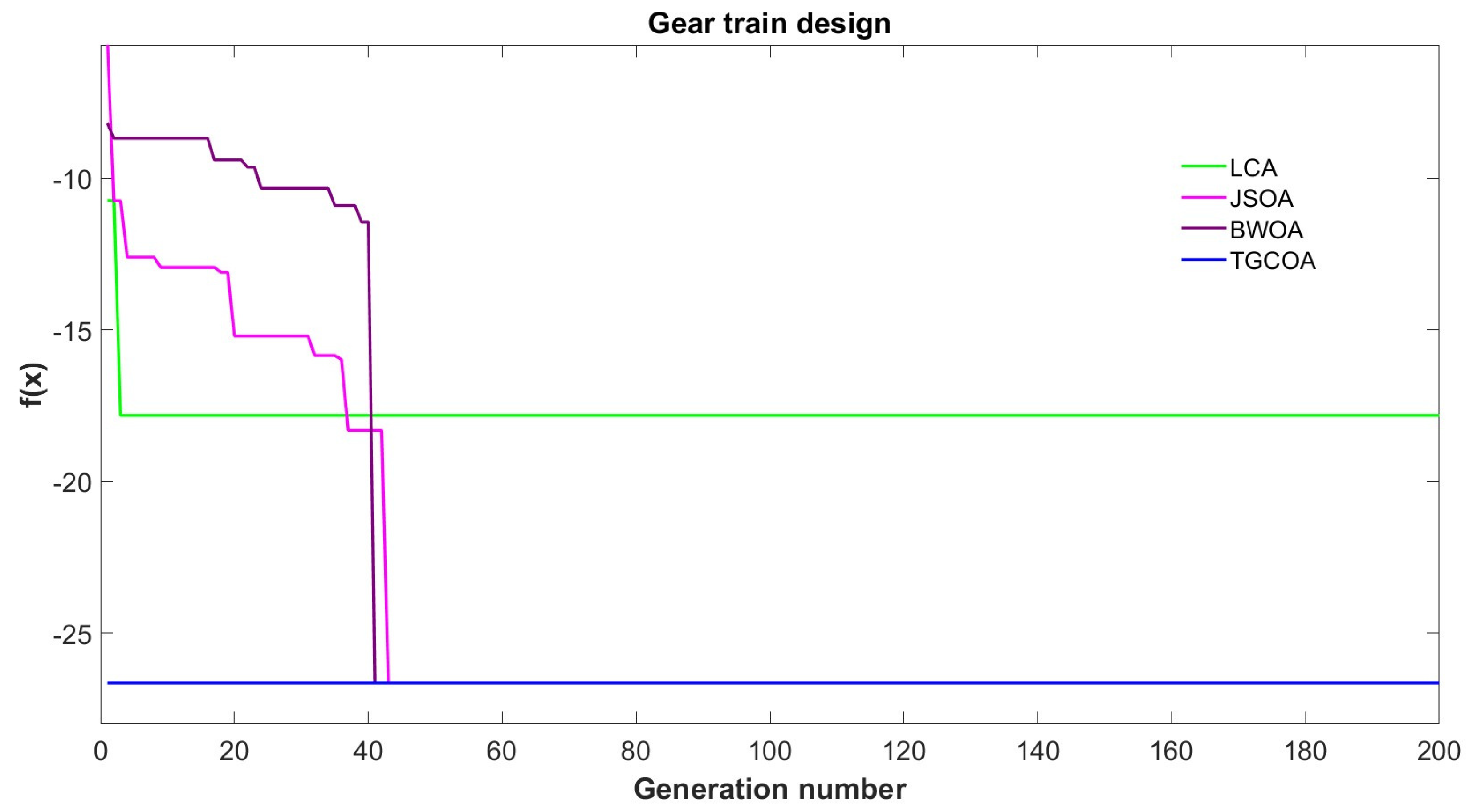
The statistical results of this test, presented in Table 26, show that all algorithms reported feasible solutions. Although the TGCOA outperformed LCA by attaining a value of 2.70 × 10 12 , it also demonstrated competitive performance compared to BWOA and JSOA. Figure 18 shows the convergence graph.

5.6. Tubular Column Design

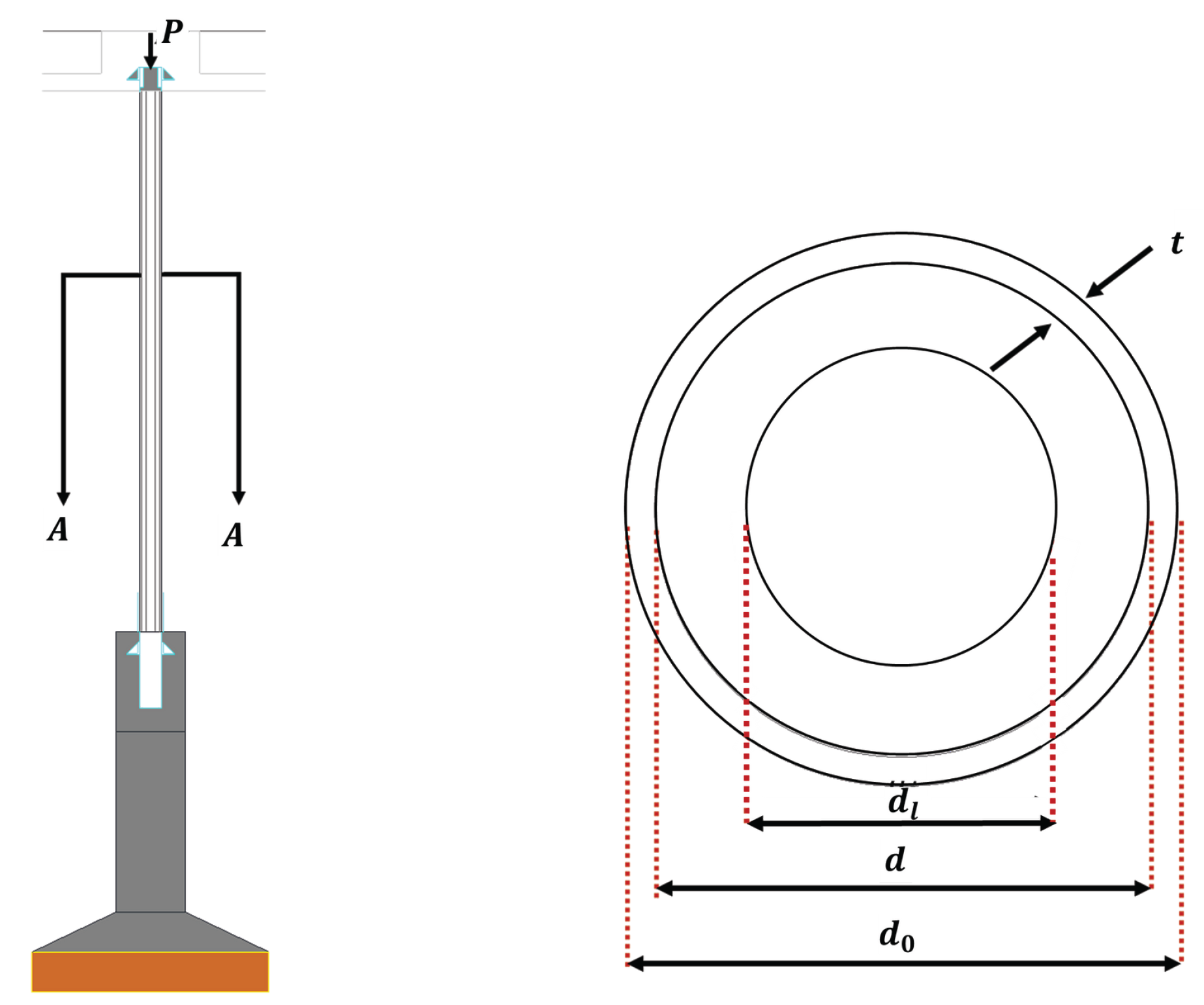
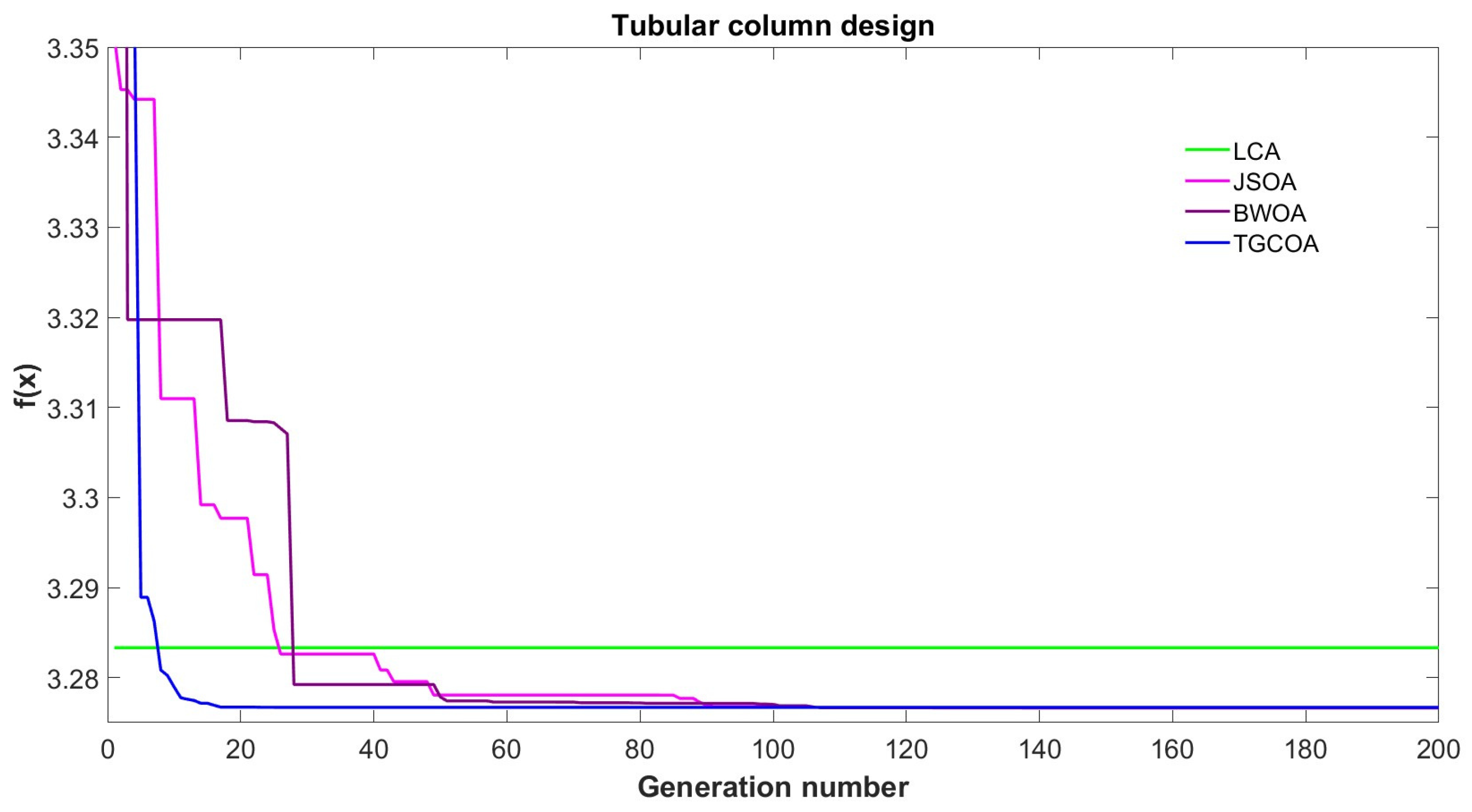
This optimization issue focuses on designing a uniform tubular column under axial compressive pressure to minimize overall material cost while maintaining structural integrity [97]. Figure 19 depicts the design variables: mean diameter d = x 1 and pipe thickness t = x 2 . The column material has a yield stress of σ y = 500 kgf / cm 2 and a modulus of elasticity E = 0.85 × 10 6 kgf / cm 2 . The mathematical formulation of the problem includes constraints that ensure that the applied stress does not exceed the buckling and creep limits ( g 1 and g 2 ), while additional constraints ( g 3 to g 6 ) limit the design variables to feasible ranges. As shown below,
Minimize : f ( X ) = 9.8 x 1 x 2 + 2 x 1 , Subject to g 1 ( X ) = P π x 1 x 2 σ y 1 0 , g 2 ( X ) = 8 P L 2 π 3 E x 1 x 2 ( x 1 2 + x 2 2 ) 1 0 , g 3 ( X ) = 2.0 x 1 1 0 , g 4 ( X ) = x 1 14 1 0 , g 5 ( X ) = 0.2 x 2 1 0 , g 6 ( X ) = x 2 8 1 0 , Variable range : 2 x 1 14 , 0.2 x 2 0.8 .
Table 27 shows that all algorithms reported feasible solutions. By attaining a value of 26.4864, the TGCOA outperformed LCA and demonstrated competitive performance for BWOA and JSOA. The convergence graph is shown in Figure 20.

5.7. Welded Beam Design

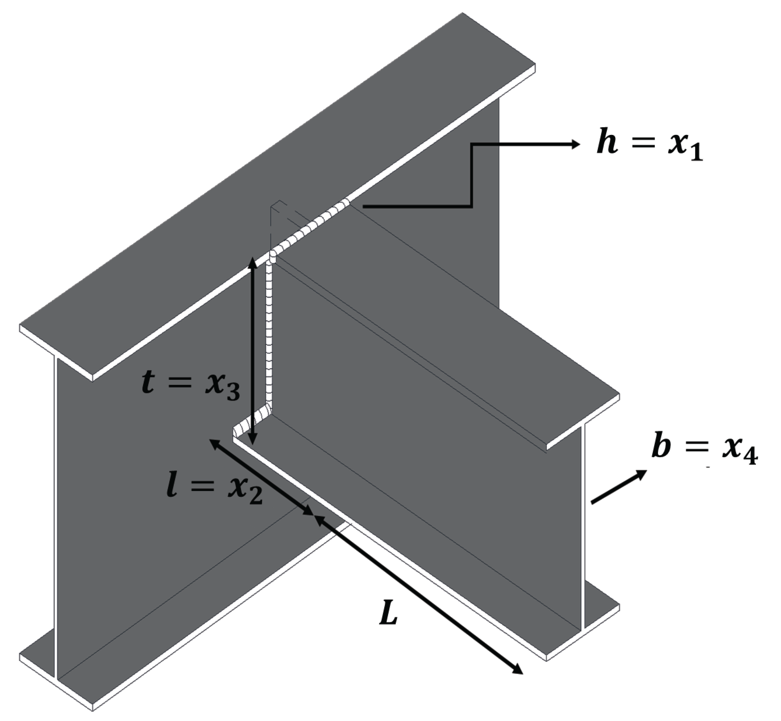
The design problem of a welded beam is a reference case initially taken from [97,100] and widely addressed in the optimization literature. As illustrated in Figure 21, the beam is subjected to a vertical load, and the main objective is to minimize the total fabrication cost. This cost considers both materials and welding processes. The model is subject to seven constraints related to stress, deflection, welding design criteria, and geometric constraints. The design variables involved are weld thickness x 1 , beam height x 2 , plate length x 3 , and cross bar thickness x 4 .
Minimize : f ( X ) = 1.10471 x 1 2 x 2 + 0.04811 x 3 x 4 14.0 + x 2 , Subject to g 1 ( X ) = τ ( X ) τ max 0 , g 2 ( X ) = σ ( X ) σ max 0 , g 3 ( X ) = δ ( X ) δ max 0 , g 4 ( X ) = x 1 x 4 0 , g 5 ( X ) = P P c ( X ) 0 , g 6 ( X ) = 0.125 x 1 0 , g 7 ( X ) = 1.10471 x 1 2 + 0.04811 x 3 x 4 ( 14.0 + x 2 ) 5.0 0 .
where
τ ( X ) = τ 2 + 2 τ τ x 2 2 R + τ 2 τ = P 2 x 1 x 2 , τ = M R J , M = P L + x 2 2 R = x 2 2 4 + x 1 + x 3 2 2 J = 2 2 x 1 x 2 x 2 2 4 + x 1 + x 3 2 2 σ ( X ) = 6 P L x 4 x 3 2 , δ ( X ) = 6 P L 3 E x 3 2 x 4 P c ( X ) = 4.013 E x 3 2 x 4 6 36 L 2 1 x 3 2 L E 4 G
Constants:
P = 6000 lb , L = 14 in , δ max = 0.25 in E = 30 × 10 6 psi , G = 12 × 10 6 psi τ max = 13 , 600 psi , σ max = 30 , 000 psi
Variable bounds: 0.1 x 1 , x 4 2 , 0.1 x 2 , x 3 10 .
Figure 21. Welded beam construction showing design variations.
Mathematics 13 02721 g021
The statistical results of this test, presented in Table 28, show that all algorithms reported feasible solutions, highlighting that the TGCOA outperforms the algorithms with which it was compared, obtaining a value of 1.7367. Figure 22 displays the corresponding convergence graph.

5.8. Reinforced Concrete Beam Design

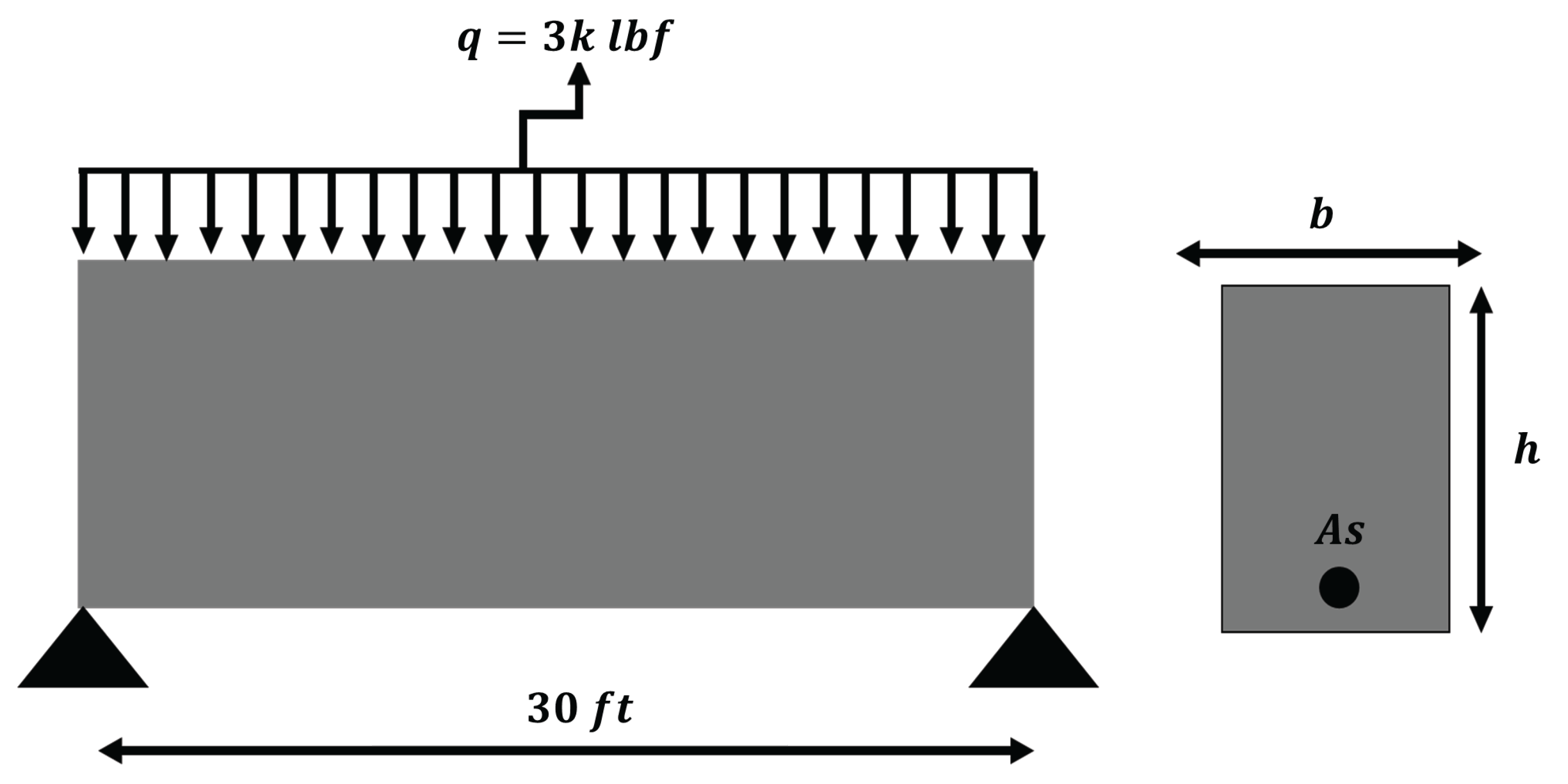
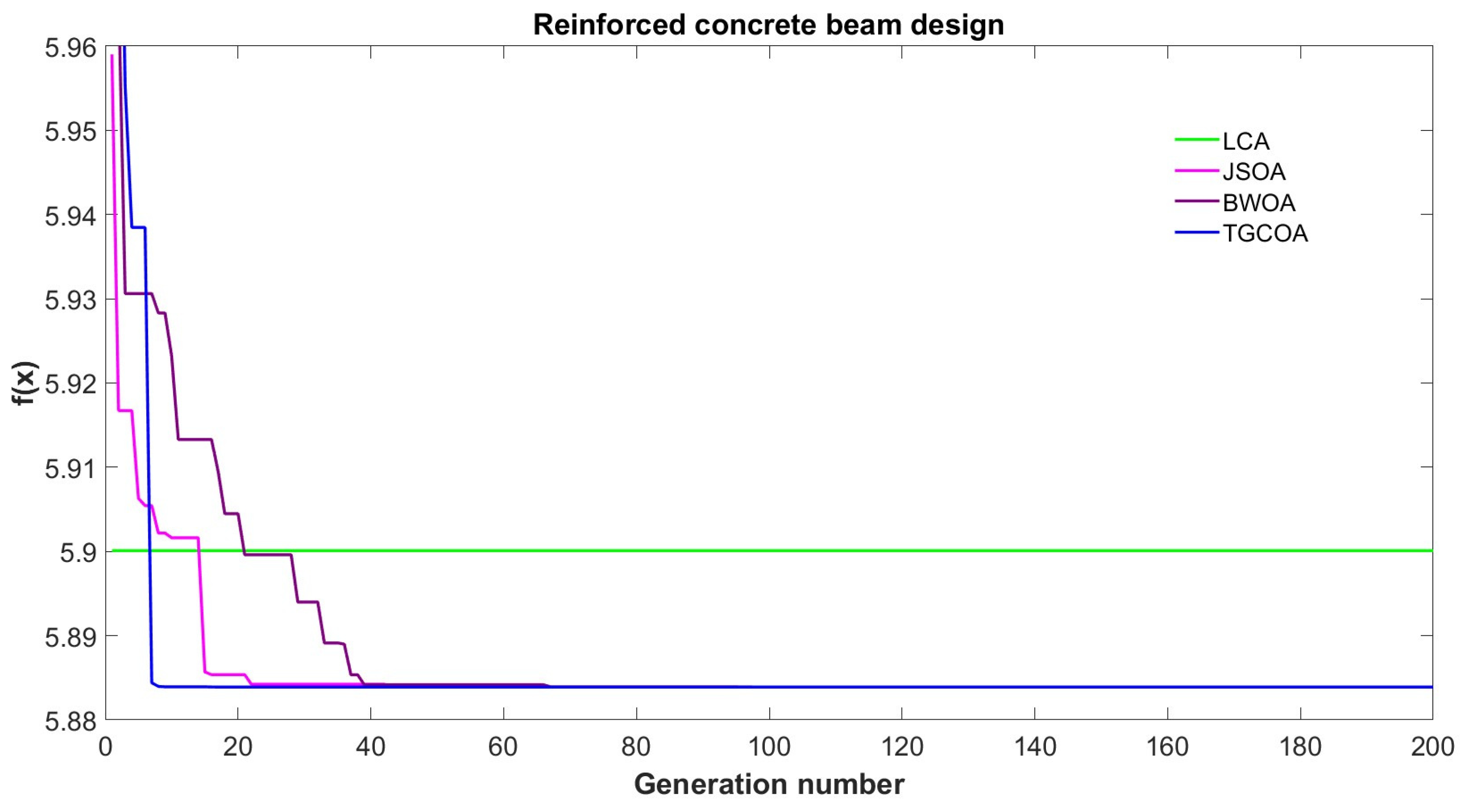
The optimization problem for the design of a reinforced concrete beam, taken from [97], is illustrated in Figure 23. A simply supported beam with a span of 9 m is considered, subjected to a live load of 900 kgf and a dead load of 450 kgf, including the self-weight of the beam. The compressive strength of the concrete is 5 ksi, while the yield strength of the reinforcing steel is 50 ksi. The cost of the concrete is estimated at USD 0.02/in2/linear ft, and that of the steel at USD 1.00/in 2/linear ft.
The objective is to minimize the total cost of the structure by determining the reinforcement area A s ( = x 1 ) , beam width b ( = x 2 ) , and beam depth h ( = x 3 ) . The design must comply with ACI 318-77 code specifications as follows: M u = 0.9 A s σ y ( 0.8 h ) 1.0 0.59 A s σ y 0.8 b h σ c 1.4 M d + 1.7 M l
In this context, M u , M a , and M 1 represent the bending resistance, the moment due to dead load, and the moment due to live load, respectively, with values of M a = 1350 in-kip and M 1 = 2700 in-kip. In addition, it is imposed that the ratio between the edge and the width of the beam does not exceed the value of 4, h b 4 . The mathematical formulation of this optimization problem is presented below.
Minimize : f ( X ) = 2.9 x 1 + 0.6 x 2 x 3 , Subject to g 1 ( X ) = x 2 x 3 4 0 , g 2 ( X ) = 180 + 7.375 x 1 2 x 3 x 1 x 2 0 , Variable range : x 1 { 6 , 6.16 , 6.32 , 6.6 , 7 , 7.11 , 7.2 , 7.8 , 7.9 , 8 , 8.4 } , x 2 { 28 , 29 , 30 , , 40 } , 5 x 3 10 .
As shown in Table 29, all algorithms reported feasible solutions. The TGCOA demonstrated competitive performance to BWOA and JSOA. Moreover, it surpassed LCA by attaining a value of 359.208. The convergence graph is shown in Figure 24.

6. Conclusions

This paper introduces a novel metaheuristic named the Tetragonula carbonaria Optimization Algorithm (TGCOA), inspired by the thermoregulatory and building behaviors of the stingless bee. The proposed approach models three behavior patterns based on hive temperature: The strategies involve strengthening the structure’s hive when it is cold, building combs in a spiral pattern at medium temperatures, and stabilizing the hive when it is hot. These temperature-dependent strategies are mathematically integrated into the algorithm to balance global exploration and local exploitation in the solution space. The algorithm’s performance was evaluated using twenty standard testbench functions, comprising ten unimodal and ten multimodal benchmarks. Additionally, twenty-eight constrained problems taken from the IEEE CEC 2017 “Constrained Real-Parameter Optimization" were used in four dimensions, 10, 30, 50, and 100, as well as seven real-world engineering design problems. The algorithm’s performance was compared against ten state-of-the-art bio-inspired algorithms: the BWOA, JSOA, LCA, EMA, BO, SSA, ALO, MAO, PSO, and DE. The Wilcoxon signed-rank and Friedman statistical tests were used to compare performance over all the algorithms.
The outcomes and conclusions of this work are summarized below:
  • The TGCOA operates without additional parameters, using only a fixed population size of 30 and only 200 iterations. Note that a low number of iterations contributes to the algorithm’s efficiency compared to several approaches reported in the literature that use more iterations.
  • According to the Wilcoxon rank-sum test results on the 20 benchmark functions, the TGCOA significantly outperformed several algorithms, including the EMA, LCA, BO, SSA, ALO, MAO, PSO, and DE. Meanwhile, no significant differences were observed compared to the BWOA and JSOA. Furthermore, the Friedman test results showed that the TGCOA was ranked first.
  • For 10-dimensional problems, the Wilcoxon rank-sum test shows that the TGCOA outperformed the BWOA and LCA, with no significant differences found when compared to the JSOA. Additionally, the Friedman test ranked the TGCOA in third place. In 30-dimensional scenarios, the Wilcoxon test indicates that the TGCOA outperformed the LCA, while no statistical differences were observed regarding the BWOA and JSOA. Nevertheless, the Friedman test positioned the TGCOA as the top-performing algorithm. When analyzing 50-dimensional problems, the Wilcoxon rank-sum test indicates that the TGCOA outperformed the BWOA and LCA, while no significant difference was found compared to the JSOA. Additionally, the Friedman test ranked the TGCOA first. At 100 dimensions, the TGCOA showed statistically superior results compared to all the other algorithms according to the Wilcoxon test. According to the Friedman test ranking, the TGCOA was placed at the top. Overall, this n-dimensional analysis demonstrates the TGCOA’s superior performance, particularly in higher-dimensional cases such as 30, 50, and 100 dimensions.
  • The Average Convergence Rate (ACR) results show that the TGCOA was categorized as excellent in the average speed at which it approaches an optimal solution (near-optimal) during its iterative process.
  • The TGCOA demonstrated competitive performance regarding engineering design problems, including gear train design, tubular column design, and reinforced concrete beam design. Meanwhile, it outperformed problems in tension/compression spring design, pressure vessel design, three-bar truss design, and welded beam design.
  • The TGCOA demonstrates the ability to effectively address constrained real-world optimization problems characterized by unknown search spaces, delivering remarkable outcomes.
The proposed algorithm demonstrated competitive performance; however, certain limitations remain, revealing opportunities for future work, such as the ability to solve multi-objective optimization problems, including a higher number of variables, optimization problems in dynamic environments, and hybrid development with other techniques, such as hyper-heuristic-based environments for designing generic methods that produce solutions of acceptable quality, incorporating low-level heuristics that improve both exploration and exploitation in the search space. Furthermore, it is necessary to analyze how population size and number of iterations affect the performance of the algorithm for Large-Scale Global Optimization Problems (LSGOs). Currently, the TGCOA is being improved for hyperparameter optimization of convolutional neural networks in medical applications.

Author Contributions

Conceptualization, M.G.M.G. and H.P.V.; methodology, M.G.M.G. and H.P.V.; software, M.G.M.G. and H.P.V.; validation, H.P.V.; formal analysis, M.G.M.G. and H.P.V.; investigation, M.G.M.G.; resources, H.P.V.; writing—original draft preparation, M.G.M.G.; writing—review and editing, H.P.V.; visualization, M.G.M.G.; supervision, H.P.V.; project administration, H.P.V.; funding acquisition, H.P.V. All authors have read and agreed to the published version of this manuscript.

Funding

This project was supported by the Instituto Politécnico Nacional (IPN) through grant SIP no. 20250569.

Data Availability Statement

The source code used to support the findings of this study has been deposited for the scientific community in the MathWorks repository at https://www.mathworks.com/matlabcentral/fileexchange/181842-algorithm-based-on-hive-construction-by-tetragonula-c-bee (accessed on 19 August 2025).

Acknowledgments

The first author acknowledges support from SECIHTI to pursue his PhD studies in advanced technology at the Instituto Politécnico Nacional (IPN)–CICATA Altamira.

Conflicts of Interest

The authors declare no potential conflicts of interest with respect to the research, authorship, funding, and/or publication of this article.

Appendix A

Table A1. Classification of 20 testbench functions.
IDFunction NameUnimodalMultimodaln-DimensionalNon-SeparableConvexDifferentiableContinuousNonconvexNon-DifferentiableSeparableRandom
F1BrownX XXXX
F2GriewankX XX XX
F3Schwefel 2.20X XX XXX
F4Schwefel 2.21X X X X XX
F5Schwefel 2.22X X X X XX
F6Schwefel 2.23X X XXX X
F7SphereX X XXX X
F8Sum SquaresX X XXX X
F9Xin-She Yang N. 3X XX X X
F10ZakharovX X X X
F11Ackley XX XXX
F12Ackley N. 4 XXX X X
F13Periodic XX XXXX
F14Quartic XX XX XX
F15Rastrigin XX XXX X
F16Rosenbrock XXX XXX
F17Salomon XXX XXX
F18Xin-She Yang XX XXX
F19Xin-She Yang N. 2 XXX XX
F20Xin-She Yang N. 4 XXX XX
Table A2. Description of the 20 testbench functions.
IDFunctionDimInterval f min
F1 f ( x ) = f x 1 , , x n = i = 1 n 1 x i 2 x i + 1 2 + 1 + x i + 1 2 x i 2 + 1 30 [ 1 , 4 ] 0
F2 f ( x ) = f x 1 , , x n = 1 + i = 1 n x i 2 4000 i = 1 n cos x i i 30 [ 600 , 600 ] 0
F3 f ( x ) = f x 1 , , x n = i = 1 n x i 30 [ 100 , 100 ] 0
F4 f ( x ) = f x 1 , , x n = max i = 1 , , n x i 30 [ 100 , 100 ] 0
F5 f ( x ) = f x 1 , , x n = i = 1 n x i + i = 1 n x i 30 [ 100 , 100 ] 0
F6 f ( x ) = f x 1 , , x n = i = 1 n x i 10 30 [ 10 , 10 ] 0
F7 f ( x ) = f x 1 , x 2 , , x n = i = 1 n x i 2 30 [ 5.12 , 5.12 ] 0
F8 f ( x ) = f x 1 , , x n = i = 1 n i x i 2 30 [ 10 , 10 ] 0
F9 f ( x ) = f x 1 , , x n = exp i = 1 n x i / β 2 m 2 exp i = 1 n x i 2 i = 1 n cos 2 x i 30 [ 2 π , 2 π ] , m = 5 ,
β = 15
-1
F10 f ( x ) = f x 1 , . . , x n = i = 1 n x i 2 + i = 1 n 0.5 i x i 2 + i = 1 n 0.5 i x i 4 30 [ 5 , 10 ] 0
F11 f ( x ) = f x 1 , , x n = a · exp b 1 n i = 1 n x i 2 exp 1 d i = 1 n cos c x i + a + exp ( 1 ) 30 [ 32 , 32 ] , a = 20
b = 0.3 , c = 2 π
0
F12 f ( x ) = f x 1 , , x n = i = 1 n 1 e 0.2 x i 2 + x i + 1 2 + 3 cos 2 x i + sin 2 x i + 1 2 [ 35 , 35 ] 5.901 × 10 14
F13 f ( x ) = f x 1 , , x n = 1 + i = 1 n sin 2 x i 0.1 e i = 1 n x i 2 30 [ 10 , 10 ] 0.9
F14 f ( x ) = f x 1 , , x n = i = 1 n i x i 4 + random [ 0 , 1 ) 30 [ 1.28 , 1.28 ] 0 + random noise
F15 f ( x , y ) = 10 n + i = 1 n x i 2 10 cos 2 π x i 30 [ 5.12 , 5.12 ] 0
F16 f x 1 x n = i = 1 n 1 100 x i 2 x i + 1 2 + 1 x i 2 30 [ 5 , 10 ] 0
F17 f ( x ) = f x 1 , , x n = 1 cos 2 π i = 1 D x i 2 + 0.1 i = 1 D x i 2 30 [ 100 , 100 ] 0
F18 f ( x ) = f x 1 , , x n = i = 1 n ϵ i x i i 30 [ 5 , 5 ] , ε random0
F19 f ( x ) = f x 1 , , x n = i = 1 n x i exp i = 1 n sin x i 2 30 [ 2 π , 2 π ] 0
F20 f ( x ) = f x 1 , , x n = i = 1 n sin 2 x i e i = 1 n x i 2 e i = 1 n sin 2 x i 30 [ 10 , 10 ] -1
Table A3. CEC 2017 Constrained Real-Parameter Optimization.
Problem/Search RangeType of ObjectiveNumber of Constraints
EI
C01Non Separable01
[ 100 , 100 ] D Separable
C02Non Separable01
[ 100 , 100 ] D Non Separable, Rotated
C03Non Separable11
[ 100 , 100 ] D SeparableSeparable
C04Separable02
[ 10 , 10 ] D Separable
C05Non Separable02
[ 10 , 10 ] D Non Separable, Rotated
C06Separable60
[ 20 , 20 ] D
C07Separable20
[ 50 , 50 ] D
C08Separable20
[ 100 , 100 ] D
C09Separable20
[ 10 , 10 ] D
C10Separable20
[ 100 , 100 ] D
C11Separable11
[ 100 , 100 ] D Non SeparableNon Separable
C12Separable02
[ 100 , 100 ] D Separable
C13Non Separable03
[ 100 , 100 ] D Separable
C14Non Separable11
[ 100 , 100 ] D SeparableSeparable
C15Separable11
[ 100 , 100 ] D
C16Separable11
[ 100 , 100 ] D Non SeparableSeparable
C17Non Separable11
[ 100 , 100 ] D Non SeparableSeparable
C18Separable12
[ 100 , 100 ] D Non Separable
C19Separable02
[ 50 , 50 ] D Non Separable
C20Non Separable02
[ 100 , 100 ] D
C21Rotated02
[ 100 , 100 ] D Rotated
C22Rotated03
[ 100 , 100 ] D Rotated
C23Rotated11
[ 100 , 100 ] D RotatedRotated
C24Rotated11
[ 100 , 100 ] D RotatedRotated
C25Rotated11
[ 100 , 100 ] D RotatedRotated
C26Rotated11
[ 100 , 100 ] D RotatedRotated
C27Rotated12
[ 100 , 100 ] D RotatedRotated
C28Rotated02
[ 50 , 50 ] D Rotated
There are 28 test cases provided, with D indicating the decision factors, I indicating inequality constraints, and E indicating equality constraints.
Table A4. ACR results for TGCOA.
FunctionACRCategory
F11Optimal
F21Optimal
F31Optimal
F41Optimal
F51Optimal
F61Optimal
F71Optimal
F81Optimal
F91Optimal
F101Optimal
F111Optimal
F12 6.08 × 10 1 Good
F131Optimal
F141Optimal
F151Optimal
F16 8.05 × 10 1 Good
F171Optimal
F181Optimal
F191Optimal
F201Optimal
The category is assigned based on the ACR value: Optimal (ACR = 1), Excellent (ACR ≥ 0.9), Good ( 0.5 ACR < 0.9 ), Slow ( 0 < ACR < 0.5 ), or No Improvement (ACR = 0).
Table A5. ACR results for JSOA.
FunctionACRCategory
F11Optimal
F21Optimal
F31Optimal
F41Optimal
F51Optimal
F61Optimal
F71Optimal
F81Optimal
F91Optimal
F101Optimal
F111Optimal
F121Optimal
F131Optimal
F141Optimal
F151Optimal
F161Optimal
F171Optimal
F181Optimal
F191Optimal
The category is assigned based on the ACR value: Optimal (ACR = 1), Excellent (ACR ≥ 0.9), Good ( 0.5 ACR < 0.9 ), Slow ( 0 < ACR < 0.5 ), or No Improvement (ACR = 0).
Table A6. ACR results for BWOA.
FunctionACRCategory
F11Optimal
F21Optimal
F31Optimal
F41Optimal
F51Optimal
F61Optimal
F71Optimal
F81Optimal
F91Optimal
F101Optimal
F111Optimal
F12 3.99 × 10 1 Slow
F131Optimal
F14 6.56 × 10 1 Good
F151Optimal
F16 4.92 × 10 1 Slow
F171Optimal
F181Optimal
F191Optimal
F201Optimal
The category is assigned based on the ACR value: Optimal (ACR = 1), Excellent (ACR ≥ 0.9), Good ( 0.5 ACR < 0.9 ), Slow ( 0 < ACR < 0.5 ), or No Improvement (ACR = 0).
Table A7. ACR results for LCA.
FunctionACRCategory
F1 3.15 × 10 1 Slow
F21Optimal
F3 5.87 × 10 1 Good
F4 7.15 × 10 1 Good
F5 4.44 × 10 1 Slow
F60No Improvement
F71Optimal
F8 3.64 × 10 1 Slow
F91Optimal
F100No Improvement
F11 2.13 × 10 1 Slow
F12 7.60 × 10 1 Good
F131Optimal
F141Optimal
F151Optimal
F161Optimal
F171Optimal
F181Optimal
F191Optimal
F201Optimal
The category is assigned based on the ACR value: Optimal (ACR = 1), Excellent (ACR ≥ 0.9), Good ( 0.5 ACR < 0.9 ), Slow ( 0 < ACR < 0.5 ), or No Improvement (ACR = 0).
Table A8. ACR results for PSO.
FunctionACRCategory
F11Optimal
F21Optimal
F31Optimal
F4 4.52 × 10 1 Slow
F51Optimal
F61Optimal
F7 1.66 × 10 1 Slow
F81Optimal
F9 3.79 × 10 1 Slow
F10 5.75 × 10 1 Good
F11 5.86 × 10 1 Good
F120No Improvement
F131Optimal
F14 3.94 × 10 1 Slow
F151Optimal
F16 9.38 × 10 1 Excellent
F171Optimal
F181Optimal
F19 3.08 × 10 1 Slow
F200No Improvement
The category is assigned based on the ACR value: Optimal (ACR = 1), Excellent (ACR ≥ 0.9), Good ( 0.5 ACR < 0.9 ), Slow ( 0 < ACR < 0.5 ), or No Improvement (ACR = 0).
Table A9. ACR results for EMA.
FunctionACRCategory
F11Optimal
F2 4.57 × 10 1 Slow
F3 6.73 × 10 1 Good
F4 7.06 × 10 1 Good
F5 6.73 × 10 1 Good
F61Optimal
F7 2.18 × 10 1 Slow
F81Optimal
F90No Improvement
F10 4.46 × 10 1 Slow
F111Optimal
F12 1.72 × 10 1 Slow
F13 4.61 × 10 1 Slow
F141Optimal
F15 3.45 × 10 1 Slow
F161Optimal
F17 6.92 × 10 1 Good
F181Optimal
F19 3.75 × 10 1 Slow
F20 6.18 × 10 1 Good
The category is assigned based on the ACR value: Optimal (ACR = 1), Excellent (ACR ≥ 0.9), Good ( 0.5 ACR < 0.9 ), Slow ( 0 < ACR < 0.5 ), or No Improvement (ACR = 0).
Table A10. ACR results for SSA.
FunctionACRCategory
F11Optimal
F21Optimal
F3 7.28 × 10 1 Good
F4 6.50 × 10 1 Good
F51Optimal
F6 4.53 × 10 1 Slow
F7 3.52 × 10 1 Slow
F8 9.66 × 10 1 Excellent
F9 2.60 × 10 1 Slow
F10 5.02 × 10 1 Good
F11 3.38 × 10 1 Slow
F121Optimal
F131Optimal
F14 2.45 × 10 1 Slow
F151Optimal
F161Optimal
F17 6.97 × 10 1 Good
F181Optimal
F191Optimal
F20 4.54 × 10 1 Slow
The category is assigned based on the ACR value: Optimal (ACR = 1), Excellent (ACR ≥ 0.9), Good ( 0.5 ACR < 0.9 ), Slow ( 0 < ACR < 0.5 ), or No Improvement (ACR = 0).
Table A11. ACR results for ALO.
FunctionACRCategory
F1 7.23 × 10 1 Good
F2 6.75 × 10 1 Good
F3 8.35 × 10 1 Good
F41Optimal
F51Optimal
F61Optimal
F7 4.83 × 10 1 Slow
F8 5.02 × 10 1 Good
F9 6.02 × 10 1 Good
F101Optimal
F11 8.38 × 10 1 Good
F121Optimal
F13 1.67 × 10 1 Slow
F141Optimal
F15 6.16 × 10 1 Good
F16 9.54 × 10 1 Excellent
F17 7.06 × 10 1 Good
F181Optimal
F190No Improvement
F201Optimal
The category is assigned based on the ACR value: Optimal (ACR = 1), Excellent (ACR ≥ 0.9), Good ( 0.5 ACR < 0.9 ), Slow ( 0 < ACR < 0.5 ), or No Improvement (ACR = 0).
Table A12. ACR results for BO.
FunctionACRCategory
F11Optimal
F21Optimal
F3 5.22 × 10 1 Good
F4 4.08 × 10 1 Slow
F5 5.76 × 10 1 Good
F61Optimal
F70No Improvement
F8 9.59 × 10 1 Excellent
F90No Improvement
F10 9.57 × 10 1 Excellent
F11 4.57 × 10 1 Slow
F120No Improvement
F13 5.41 × 10 1 Good
F141Optimal
F15 4.58 × 10 1 Slow
F161Optimal
F17 7.32 × 10 1 Good
F181Optimal
F190No Improvement
F20 8.65 × 10 1 Good
The category is assigned based on the ACR value: Optimal (ACR = 1), Excellent (ACR ≥ 0.9), Good ( 0.5 ACR < 0.9 ), Slow ( 0 < ACR < 0.5 ), or No Improvement (ACR = 0).
Table A13. ACR results for MAO.
FunctionACRCategory
F11Optimal
F2 6.37 × 10 1 Good
F3 6.40 × 10 1 Good
F4 5.83 × 10 1 Good
F51Optimal
F61Optimal
F7 4.95 × 10 1 Slow
F81Optimal
F91Optimal
F101Optimal
F111Optimal
F121Optimal
F13 4.48 × 10 1 Slow
F14 7.61 × 10 1 Good
F15 6.13 × 10 1 Good
F16 2.95 × 10 1 Slow
F17 3.93 × 10 1 Slow
F181Optimal
F191Optimal
F201Optimal
The category is assigned based on the ACR value: Optimal (ACR = 1), Excellent (ACR ≥ 0.9), Good ( 0.5 ACR < 0.9 ), Slow ( 0 < ACR < 0.5 ), or No Improvement (ACR = 0).
Table A14. ACR results for DE.
FunctionACRCategory
F11Optimal
F2 4.44 × 10 1 Slow
F3 4.09 × 10 1 Slow
F4 2.81 × 10 1 Slow
F5 4.39 × 10 1 Slow
F61Optimal
F7 4.67 × 10 1 Slow
F8 4.06 × 10 1 Slow
F9 3.98 × 10 1 Slow
F101Optimal
F11 3.83 × 10 1 Slow
F12 8.17 × 10 1 Good
F13 5.94 × 10 1 Good
F14 3.41 × 10 1 Slow
F15 7.38 × 10 1 Good
F16 7.03 × 10 1 Good
F17 4.64 × 10 1 Slow
F181Optimal
F191Optimal
F20 4.97 × 10 1 Slow
The category is assigned based on the ACR value: Optimal (ACR = 1), Excellent (ACR ≥ 0.9), Good ( 0.5 ACR < 0.9 ), Slow ( 0 < ACR < 0.5 ), or No Improvement (ACR = 0).
Table A15. Preparatory work for implementing TGCOA.
StepDescription
1.Parameter definition: population size, number of iterations, and the upper and lower bounds for each variable.
2.Provide objective function to minimize/maximize, as well as equality and inequality constraints of the problem.
3.Define the handling constraint method to be applied.
4.The algorithm starts by executing the script named main. The TGCOA’s MATLAB code is available to support this study’s findings.
5.To obtain reliable results, it is recommended to run the algorithm at least 30 times using benchmark functions with known optimal values. Calculate the best value found, the mean, and the standard deviation to determine how close or far the achieved result is compared to the known optimal value. Additionally, apply non-parametric statistical tests to validate the results.
Figure A1. The ACR plots for the algorithms.
Mathematics 13 02721 g0a1

References

  1. Peraza-Vázquez, H.; Peña-Delgado, A.; Merino-Treviño, M.; Morales-Cepeda, A.B.; Sinha, N. A novel metaheuristic inspired by horned lizard defense tactics. Artif. Intell. Rev. 2024, 57, 59. [Google Scholar] [CrossRef]
  2. Holland, J.H. Genetic Algorithms and the Optimal Allocation of Trials. SIAM J. Comput. 1973, 2, 88–105. [Google Scholar] [CrossRef]
  3. Alhijawi, B.; Awajan, A. Genetic algorithms: Theory, genetic operators, solutions, and applications. Evol. Intell. 2024, 17, 1245–1256. [Google Scholar] [CrossRef]
  4. Maheri, A.; Jalili, S.; Hosseinzadeh, Y.; Khani, R.; Miryahyavi, M. A comprehensive survey on cultural algorithms. Swarm Evol. Comput. 2021, 62, 100846. [Google Scholar] [CrossRef]
  5. Ahrari, A.; Essam, D. An Introduction to Evolutionary and Memetic Algorithms for Parameter Optimization. In Evolutionary and Memetic Computing for Project Portfolio Selection and Scheduling; Harrison, K.R., Elsayed, S., Garanovich, I.L., Weir, T., Boswell, S.G., Sarker, R.A., Eds.; Springer International Publishing: Cham, Switzerland, 2022; pp. 37–63. [Google Scholar] [CrossRef]
  6. Zhong, J.; Feng, L.; Ong, Y.S. Gene Expression Programming: A Survey [Review Article]. IEEE Comput. Intell. Mag. 2017, 12, 54–72. [Google Scholar] [CrossRef]
  7. Beyer, H.G.; Schwefel, H.P. Evolution strategies—A comprehensive introduction. Nat. Comput. 2002, 1, 3–52. [Google Scholar] [CrossRef]
  8. Kim, C.; Lee, B. TORCWA: GPU-accelerated Fourier modal method and gradient-based optimization for metasurface design. Comput. Phys. Commun. 2023, 282, 108552. [Google Scholar] [CrossRef]
  9. Storn, R.; Price, K. Differential Evolution—A Simple and Efficient Heuristic for global Optimization over Continuous Spaces. J. Glob. Optim. 1997, 11, 341–359. [Google Scholar] [CrossRef]
  10. Houssein, E.H.; Oliva, D.; Samee, N.A.; Mahmoud, N.F.; Emam, M.M. Liver Cancer Algorithm: A novel bio-inspired optimizer. Comput. Biol. Med. 2023, 165, 107389. [Google Scholar] [CrossRef]
  11. Sulaiman, M.H.; Mustaffa, Z.; Saari, M.M.; Daniyal, H.; Mirjalili, S. Evolutionary mating algorithm. Neural Comput. Appl. 2022, 35, 487–516. [Google Scholar] [CrossRef]
  12. Chaipornkaew, P.; Banditwattanawong, T. A Novel Method for News Recommendation on Websites Using the Clustered-Vectors Optimization Algorithm. IEEE Access 2025, 13, 6685–6703. [Google Scholar] [CrossRef]
  13. Kennedy, J.; Eberhart, R. Particle swarm optimization. In Proceedings of the ICNN’95—International Conference on Neural Networks, Perth, WA, Australia, 27 November–1 December 1995; Volume 4, pp. 1942–1948. [Google Scholar] [CrossRef]
  14. Chopra, N.; Ansari, M.M. Golden jackal optimization: A novel nature-inspired optimizer for engineering applications. Expert Syst. Appl. 2022, 198, 116924. [Google Scholar] [CrossRef]
  15. Peraza-Vázquez, H.; Peña-Delgado, A.; Ranjan, P.; Barde, C.; Choubey, A.; Morales-Cepeda, A.B. A Bio-Inspired Method for Mathematical Optimization Inspired by Arachnida Salticidade. Mathematics 2021, 10, 102. [Google Scholar] [CrossRef]
  16. Peña-Delgado, A.F.; Peraza-Vázquez, H.; Almazán-Covarrubias, J.H.; Torres-Cruz, N.; García-Vite, P.M.; Morales-Cepeda, A.B.; Ramirez-Arredondo, J.M. Corrigendum to “A Novel Bio-Inspired Algorithm Applied to Selective Harmonic Elimination in a Three-Phase Eleven-Level Inverter”. Math. Probl. Eng. 2022, 2022, 9808273. [Google Scholar] [CrossRef]
  17. Trojovska, E.; Dehghani, M.; Trojovsky, P. Fennec Fox Optimization: A New Nature-Inspired Optimization Algorithm. IEEE Access 2022, 10, 84417–84443. [Google Scholar] [CrossRef]
  18. Peraza-Vázquez, H.; Peña-Delgado, A.F.; Echavarría-Castillo, G.; Morales-Cepeda, A.B.; Velasco-Álvarez, J.; Ruiz-Perez, F. A Bio-Inspired Method for Engineering Design Optimization Inspired by Dingoes Hunting Strategies. Math. Probl. Eng. 2021, 2021, 1–19. [Google Scholar] [CrossRef]
  19. Wang, L.; Cao, Q.; Zhang, Z.; Mirjalili, S.; Zhao, W. Artificial rabbits optimization: A new bio-inspired meta-heuristic algorithm for solving engineering optimization problems. Eng. Appl. Artif. Intell. 2022, 114, 105082. [Google Scholar] [CrossRef]
  20. Kaur, S.; Awasthi, L.K.; Sangal, A.; Dhiman, G. Tunicate Swarm Algorithm: A new bio-inspired based metaheuristic paradigm for global optimization. Eng. Appl. Artif. Intell. 2020, 90, 103541. [Google Scholar] [CrossRef]
  21. Rodríguez, A.; Cortez, J.A.S.; Vázquez, H.P.; Fermin, A.; Delgado, P.; Mx, A.F.P.D. A Novel Bio-Inspired Optimization Algorithm Based on Mantis Shrimp Survival Tactics. Mathematics 2025, 13, 1500. [Google Scholar] [CrossRef]
  22. Yang, T.; Fang, J.; Jia, C.; Liu, Z.; Liu, Y. An improved harris hawks optimization algorithm based on chaotic sequence and opposite elite learning mechanism. PLoS ONE 2023, 18, e0281636. [Google Scholar] [CrossRef]
  23. Das, A.K.; Pratihar, D.K. A New Bonobo optimizer (BO) for Real-Parameter optimization. In Proceedings of the 2019 IEEE Region 10 Symposium (TENSYMP), Kolkata, India, 7–9 June 2019; pp. 108–113. [Google Scholar] [CrossRef]
  24. Mirjalili, S.; Gandomi, A.H.; Mirjalili, S.Z.; Saremi, S.; Faris, H.; Mirjalili, S.M. Salp Swarm Algorithm: A bio-inspired optimizer for engineering design problems. Adv. Eng. Softw. 2017, 114, 163–191. [Google Scholar] [CrossRef]
  25. Mirjalili, S. The Ant Lion Optimizer. Adv. Eng. Softw. 2015, 83, 80–98. [Google Scholar] [CrossRef]
  26. Villuendas-Rey, Y.; Velázquez-Rodríguez, J.L.; Alanis-Tamez, M.D.; Moreno-Ibarra, M.A.; Yáñez-Márquez, C. Mexican Axolotl Optimization: A Novel Bioinspired Heuristic. Mathematics 2021, 9, 781. [Google Scholar] [CrossRef]
  27. Abdollahzadeh, B.; Gharehchopogh, F.S.; Khodadadi, N.; Mirjalili, S. Mountain Gazelle Optimizer: A new Nature-inspired Metaheuristic Algorithm for Global Optimization Problems. Adv. Eng. Softw. 2022, 174, 103282. [Google Scholar] [CrossRef]
  28. Harifi, S.; Mohammadzadeh, J.; Khalilian, M.; Ebrahimnejad, S. Giza Pyramids Construction: An ancient-inspired metaheuristic algorithm for optimization. Evol. Intell. 2021, 14, 1743–1761. [Google Scholar] [CrossRef]
  29. Wang, L.; Du, H.; Zhang, Z.; Hu, G.; Mirjalili, S.; Khodadadi, N.; Hussien, A.G.; Liao, Y.; Zhao, W. Tianji’s horse racing optimization (THRO): A new metaheuristic inspired by ancient wisdom and its engineering optimization applications. Artif. Intell. Rev. 2025, 58, 282. [Google Scholar] [CrossRef]
  30. El-kenawy, E.S.M.; Abdelhamid, A.A.; Ibrahim, A.; Mirjalili, S.; Khodadad, N.; AI duailij, M.A.; Alhussan, A.A.; Khafaga, D.S. Al-Biruni Earth Radius (BER) Metaheuristic Search Optimization Algorithm. Comput. Syst. Sci. Eng. 2023, 45, 1917–1934. [Google Scholar] [CrossRef]
  31. Guan, Z.; Ren, C.; Niu, J.; Wang, P.; Shang, Y. Great Wall Construction Algorithm: A novel meta-heuristic algorithm for engineer problems. Expert Syst. Appl. 2023, 233, 120905. [Google Scholar] [CrossRef]
  32. Niu, J.T.; Ren, C.; Guan, Z.; Cao, Z. Dujiangyan irrigation system optimization (DISO): A novel metaheuristic algorithm for dam safety monitoring. Structures 2023, 54, 399–419. [Google Scholar] [CrossRef]
  33. Duan, X.; Hou, P. Research on Teaching Quality Evaluation Model of Physical Education Based on Simulated Annealing Algorithm. Mob. Inf. Syst. 2021, 2021, 1–8. [Google Scholar] [CrossRef]
  34. Mittal, H.; Tripathi, A.; Pandey, A.C.; Pal, R. Gravitational search algorithm: A comprehensive analysis of recent variants. Multimed. Tools Appl. 2021, 80, 7581–7608. [Google Scholar] [CrossRef]
  35. Kaveh, A.; Dadras, A. A novel meta-heuristic optimization algorithm: Thermal exchange optimization. Adv. Eng. Softw. 2017, 110, 69–84. [Google Scholar] [CrossRef]
  36. Dehghani, M.; Samet, H. Momentum search algorithm: A new meta-heuristic optimization algorithm inspired by momentum conservation law. SN Appl. Sci. 2020, 2, 1720. [Google Scholar] [CrossRef]
  37. Abdel-Basset, M.; Mohamed, R.; Sallam, K.M.; Chakrabortty, R.K. Light Spectrum Optimizer: A Novel Physics-Inspired Metaheuristic Optimization Algorithm. Mathematics 2022, 10, 3466. [Google Scholar] [CrossRef]
  38. Abdel-Basset, M.; Mohamed, R.; Azeem, S.A.A.; Jameel, M.; Abouhawwash, M. Kepler optimization algorithm: A new metaheuristic algorithm inspired by Kepler’s laws of planetary motion. Knowl.-Based Syst. 2023, 268, 110454. [Google Scholar] [CrossRef]
  39. Cheng, M.Y.; Sholeh, M.N. Artificial satellite search: A new metaheuristic algorithm for optimizing truss structure design and project scheduling. Appl. Math. Model. 2025, 143, 116008. [Google Scholar] [CrossRef]
  40. Almufti, S. Vibrating Particles System Algorithm: Overview, Modifications and Applications. ICONTECH Int. J. 2022, 6, 1–11. [Google Scholar] [CrossRef]
  41. Lam, A.Y.S.; Li, V.O.K. Chemical Reaction Optimization: A tutorial. Memetic Comput. 2012, 4, 3–17. [Google Scholar] [CrossRef]
  42. Rodan, A.; Al-Tamimi, A.K.; Al-Alnemer, L.; Mirjalili, S.; Tiňo, P. Enzyme action optimizer: A novel bio-inspired optimization algorithm. J. Supercomput. 2025, 81, 1–94. [Google Scholar] [CrossRef]
  43. Talatahari, S.; Azizi, M. Chaos Game Optimization: A novel metaheuristic algorithm. Artif. Intell. Rev. 2021, 54, 917–1004. [Google Scholar] [CrossRef]
  44. Mousavi, S.T.; Gulpen, J.G.M.; Graef, W.A.A.D.; Koelman, P.M.J.; Carbone, E.A.D.; van Dijk, J. Assessment of the suitability of the chemical reaction pathway algorithm as a reduction method for plasma chemistry. J. Phys. D Appl. Phys. 2022, 55, 505201. [Google Scholar] [CrossRef]
  45. Dehghani, M.; Trojovská, E.; Zuščák, T. A new human-inspired metaheuristic algorithm for solving optimization problems based on mimicking sewing training. Sci. Rep. 2022, 12, 17387. [Google Scholar] [CrossRef] [PubMed]
  46. Yuan, Y.; Shen, Q.; Wang, S.; Ren, J.; Yang, D.; Yang, Q.; Fan, J.; Mu, X. Coronavirus Mask Protection Algorithm: A New Bio-inspired Optimization Algorithm and Its Applications. J. Bionic Eng. 2023, 20, 1747–1765. [Google Scholar] [CrossRef] [PubMed]
  47. Emami, H. Stock exchange trading optimization algorithm: A human-inspired method for global optimization. J. Supercomput. 2022, 78, 2125–2174. [Google Scholar] [CrossRef]
  48. Hamadneh, T.; Batiha, B.; Gharib, G.M.; Montazeri, Z.; Dehghani, M.; Aribowo, W.; Noori, H.M.; Jawad, R.K.; Ibraheem, I.K. Revolution Optimization Algorithm: A New Human-based Metaheuristic Algorithm for Solving Optimization Problems. Int. J. Intell. Eng. Syst. 2025, 18, 520–531. [Google Scholar] [CrossRef]
  49. Dehghani, M.; Trojovský, P. Osprey optimization algorithm: A new bio-inspired metaheuristic algorithm for solving engineering optimization problems. Front. Mech. Eng. 2023, 8, 1126450. [Google Scholar] [CrossRef]
  50. Abdelhamid, A.A.; Towfek, S.K.; Khodadadi, N.; Alhussan, A.A.; Khafaga, D.S.; Eid, M.M.; Ibrahim, A. Waterwheel Plant Algorithm: A Novel Metaheuristic Optimization Method. Processes 2023, 11, 1502. [Google Scholar] [CrossRef]
  51. Pan, J.S.; Zhang, S.Q.; Chu, S.C.; Yang, H.M.; Yan, B. Willow Catkin Optimization Algorithm Applied in the TDOA-FDOA Joint Location Problem. Entropy 2023, 25, 171. [Google Scholar] [CrossRef]
  52. Khan, M.S.; Anwar ul Hassan, C.H.; Sadiq, H.A.; Ali, I.; Rauf, A.; Javaid, N. A New Meta-heuristic Optimization Algorithm Inspired from Strawberry Plant for Demand Side Management in Smart Grid. In Advances in Intelligent Networking and Collaborative Systems, Proceedings of the 9th International Conference on Intelligent Networking and Collaborative Systems (INCoS-2017), Toronto, ON, Canada, 24–26 August 2017; Barolli, L., Woungang, I., Hussain, O.K., Eds.; Springer: Cham, Switzerland, 2018; pp. 143–154. [Google Scholar]
  53. Kaveh, A.; Talatahari, S.; Khodadadi, N. Stochastic paint optimizer: Theory and application in civil engineering. Eng. Comput. 2022, 38, 1921–1952. [Google Scholar] [CrossRef]
  54. Zaeimi, M.; Ghoddosian, A. Color harmony algorithm: An art-inspired metaheuristic for mathematical function optimization. Soft Comput. 2020, 24, 12027–12066. [Google Scholar] [CrossRef]
  55. Patil, S.; S, S.H.; N, B.; N, D. Puzzle Optimization Algorithm based Weighted Feature Selection for Identification of Rice Leaf Disease Through Thermal Images. In Proceedings of the 2022 Smart Technologies, Communication and Robotics (STCR), Sathyamangalam, India, 10–11 December 2022; pp. 1–5. [Google Scholar] [CrossRef]
  56. Ma, B.; Hu, Y.; Lu, P.; Liu, Y. Running city game optimizer: A game-based metaheuristic optimization algorithm for global optimization. J. Comput. Des. Eng. 2023, 10, 65–107. [Google Scholar] [CrossRef]
  57. Yuan, Y.; Ren, J.; Wang, S.; Wang, Z.; Mu, X.; Zhao, W. Alpine skiing optimization: A new bio-inspired optimization algorithm. Adv. Eng. Softw. 2022, 170, 103158. [Google Scholar] [CrossRef]
  58. Chen, Y.; Wang, G.; Yin, B.; Ma, C.; Wu, Z.; Gao, M. Basketball team optimization algorithm (BTOA): A novel sport-inspired meta-heuristic optimizer for engineering applications. Sci. Rep. 2025, 15, 21629. [Google Scholar] [CrossRef] [PubMed]
  59. Kashan, A.H.; Karimiyan, S.; Kulkarni, A.J. The Golf Sport Inspired Search metaheuristic algorithm and the game theoretic analysis of its operators’ effectiveness. Soft Comput. 2024, 28, 1073–1125. [Google Scholar] [CrossRef]
  60. Abualigah, L.; Diabat, A.; Mirjalili, S.; Elaziz, M.A.; Gandomi, A.H. The Arithmetic Optimization Algorithm. Comput. Methods Appl. Mech. Eng. 2021, 376, 113609. [Google Scholar] [CrossRef]
  61. Xiao, W.; Ouyang, K.; Lian, J.J.; Gu, S.; Liu, Y.; Wei, D.; Sha, X.; Wang, J.; Fu, S.; Qiu, M.; et al. Newton Downhill Optimizer for Global Optimization. Res. Sq. 2025. [Google Scholar] [CrossRef]
  62. Kalita, K.; Ramesh, J.V.N.; Cepova, L.; Pandya, S.B.; Jangir, P.; Abualigah, L. Multi-objective exponential distribution optimizer (MOEDO): A novel math-inspired multi-objective algorithm for global optimization and real-world engineering design problems. Sci. Rep. 2024, 14, 1816. [Google Scholar] [CrossRef]
  63. Yu, C.; Lahrichi, N.; Matta, A. Optimal budget allocation policy for tabu search in stochastic simulation optimization. Comput. Oper. Res. 2023, 150, 106046. [Google Scholar] [CrossRef]
  64. Shami, T.M.; Grace, D.; Burr, A.; Mitchell, P.D. Single candidate optimizer: A novel optimization algorithm. Evol. Intell. 2024, 17, 863–887. [Google Scholar] [CrossRef]
  65. Dellaert, N.; Jeunet, J. A variable neighborhood search algorithm for the surgery tactical planning problem. Comput. Oper. Res. 2017, 84, 216–225. [Google Scholar] [CrossRef]
  66. Xu, H.; Lu, Y.; Guo, Q. Application of Improved Butterfly Optimization Algorithm Combined with Black Widow Optimization in Feature Selection of Network Intrusion Detection. Electronics 2022, 11, 3531. [Google Scholar] [CrossRef]
  67. Tan, W.H.; Mohamad-Saleh, J. A hybrid whale optimization algorithm based on equilibrium concept. Alex. Eng. J. 2023, 68, 763–786. [Google Scholar] [CrossRef]
  68. Ikram, R.M.A.; Dehrashid, A.A.; Zhang, B.; Chen, Z.; Le, B.N.; Moayedi, H. A novel swarm intelligence: Cuckoo optimization algorithm (COA) and SailFish optimizer (SFO) in landslide susceptibility assessment. Stoch. Environ. Res. Risk Assess. 2023, 37, 1717–1743. [Google Scholar] [CrossRef]
  69. Almazán-Covarrubias, J.H.; Peraza-Vázquez, H.; Peña-Delgado, A.F.; García-Vite, P.M. An Improved Dingo Optimization Algorithm Applied to SHE-PWM Modulation Strategy. Appl. Sci. 2022, 12, 992. [Google Scholar] [CrossRef]
  70. Khodadadi, N.; Harati, E.; Caso, F.D.; Nanni, A. Optimizing Truss Structures Using Composite Materials under Natural Frequency Constraints with a New Hybrid Algorithm Based on Cuckoo Search and Stochastic Paint Optimizer (CSSPO). Buildings 2023, 13, 1551. [Google Scholar] [CrossRef]
  71. Yuan, Y.; Mu, X.; Shao, X.; Ren, J.; Zhao, Y.; Wang, Z. Optimization of an auto drum fashioned brake using the elite opposition-based learning and chaotic k-best gravitational search strategy based grey wolf optimizer algorithm. Appl. Soft Comput. 2022, 123, 108947. [Google Scholar] [CrossRef]
  72. Pratha, S.J.; Asanambigai, V.; Mugunthan, S.R. Hybrid Mutualism Mechanism-Inspired Butterfly and Flower Pollination Optimization Algorithm for Lifetime Improving Energy-Efficient Cluster Head Selection in WSNs. Wirel. Pers. Commun. 2023, 128, 1567–1601. [Google Scholar] [CrossRef]
  73. Kusuma, P.D.; Dinimaharawati, A. Hybrid Pelican Komodo Algorithm. Int. J. Adv. Comput. Sci. Appl. 2022, 13, 46–55. [Google Scholar] [CrossRef]
  74. Joyce, T.; Herrmann, J.M. A Review of No Free Lunch Theorems, and Their Implications for Metaheuristic Optimisation. In Nature-Inspired Algorithms and Applied Optimization; Yang, X.S., Ed.; Springer International Publishing: Cham, Switzerland, 2018; pp. 27–51. [Google Scholar] [CrossRef]
  75. Heard, T.A. The role of stingless bees in crop pollination. Annu. Rev. Entomol. 1999, 44, 183–206. [Google Scholar] [CrossRef]
  76. Franck, P.; Cameron, E.; Good, G.; Rasplus, J.; Oldroyd, B.P. Nest architecture and genetic differentiation in a species complex of Australian stingless bees. Mol. Ecol. 2004, 13, 2317–2331. [Google Scholar] [CrossRef]
  77. Rasmussen, C. Catalog of the Indo-Malayan/Australasian stingless bees (Hymenoptera: Apidae: Meliponini). Zootaxa 2008, 1935, 1–80. [Google Scholar] [CrossRef]
  78. Brito, R.M.; Schaerf, T.M.; Myerscough, M.R.; Heard, T.A.; Oldroyd, B.P. Brood comb construction by the stingless bees Tetragonula hockingsi and Tetragonula carbonaria. Swarm Intell. 2012, 6, 151–176. [Google Scholar] [CrossRef]
  79. Halcroft, M.; Spooner-Hart, R.; Dollin, L.A. Australian Stingless Bees. In Pot-Honey; Gill, R.J., Milne, J.R.S., Eds.; Springer: New York, NY, USA, 2013; pp. 35–72. [Google Scholar] [CrossRef]
  80. Dollin, A.E.; Dollin, L.J.; Sakagami, S.F. Australian stingless bees of the genus Trigona (Hymenoptera: Apidae). Invertebr. Syst. 1997, 11, 861. [Google Scholar] [CrossRef]
  81. Smith, J.P.; Heard, T.A.; Beekman, M.; Gloag, R. Flight range of the Australian stingless bee Tetragonula carbonaria (Hymenoptera: Apidae). Austral Entomol. 2017, 56, 50–53. [Google Scholar] [CrossRef]
  82. Godeau, U.; Pioz, M.; Martin, O.; Rüger, C.; Crauser, D.; Conte, Y.L.; Henry, M.; Alaux, C. Brood thermoregulation effectiveness is positively linked to the amount of brood but not to the number of bees in honeybee colonies. Peer Community J. 2023, 3, e42. [Google Scholar] [CrossRef]
  83. Withaningsih, S.; Diaz, F.; Rozi, F.; Parikesit, P. Distribution and Characteristics of Two Species of Stingless Bee Hives (Tetragonula spp.) in the Rural Landscape of Sumedang Regency (Indonesia). Diversity 2023, 15, 1018. [Google Scholar] [CrossRef]
  84. Cardoso, S.S.S.; Cartwright, J.H.E.; Checa, A.G.; Escribano, B.; Osuna-Mascaró, A.J.; Sainz-Díaz, C.I. The bee Tetragonula builds its comb like a crystal. J. R. Soc. Interface 2020, 17, 20200187. [Google Scholar] [CrossRef]
  85. Ball, P. Pattern Formation in Nature: Physical Constraints and Self-Organising Characteristics. Archit. Des. 2012, 82, 22–27. [Google Scholar] [CrossRef]
  86. Avarguès-Weber, A.; Dyer, A.G.; Combe, M.; Giurfa, M. Simultaneous mastering of two abstract concepts by the miniature brain of bees. Proc. Natl. Acad. Sci. USA 2012, 109, 7481–7486. [Google Scholar] [CrossRef]
  87. Barron, A.B.; Klein, C. What insects can tell us about the origins of consciousness. Proc. Natl. Acad. Sci. USA 2016, 113, 4900–4908. [Google Scholar] [CrossRef]
  88. Starks, P.T.; Johnson, R.N.; Siegel, A.J.; Decelle, M.M. Heat shielding: A task for youngsters. Behav. Ecol. 2004, 16, 128–132. [Google Scholar] [CrossRef]
  89. da Silva, C.R.B.; Macnaughtan, L.D.; Griffith, O.W.; Narendra, A. Before the brink: Sublethal impacts of climate change on stingless bee flight performance. bioRxiv 2024. [Google Scholar] [CrossRef]
  90. Zemansky, M. Heat and Thermodynamics: An Intermediate Textbook, International student ed; McGraw-Hill: Boston, MA, USA, 1968. [Google Scholar]
  91. Heard, T.; Hendrikz, J. Factors Influencing Flight Activity of Colonies of the Stingless Bee Trigona-Carbonaria (Hymenoptera, Apidae). Aust. J. Zool. 1993, 41, 343. [Google Scholar] [CrossRef]
  92. Norgate, M.; Boyd-Gerny, S.; Simonov, V.; Rosa, M.G.P.; Heard, T.A.; Dyer, A.G. Ambient Temperature Influences Australian Native Stingless Bee (Trigona carbonaria) Preference for Warm Nectar. PLoS ONE 2010, 5, e12000. [Google Scholar] [CrossRef] [PubMed]
  93. Nacko, S.; Hall, M.; Duncan, M.; Cook, J.; Riegler, M.; Spooner-Hart, R. Scientific note on small hive beetle infestation of stingless bee (Tetragonula carbonaria) colony following a heat wave. Apidologie 2020, 51, 1199–1201. [Google Scholar] [CrossRef]
  94. Wu, G.; Mallipeddi, R.; Suganthan, P.N. Problem Definitions and Evaluation Criteria for the CEC 2017 Competition on Constrained Real-Parameter Optimization; Technical Report; National University of Defense Technology: Changsha, China; Kyungpook National University: Daegu, Republic of Korea; Nanyang Technological University: Singapore, 2017; Volume 9, p. 2017. [Google Scholar]
  95. He, J.; Lin, G. Average Convergence Rate of Evolutionary Algorithms. IEEE Trans. Evol. Comput. 2016, 20, 316–321. [Google Scholar] [CrossRef]
  96. Chen, Y.; He, J. Average convergence rate of evolutionary algorithms in continuous optimization. Inf. Sci. 2021, 562, 200–219. [Google Scholar] [CrossRef]
  97. Bayzidi, H.; Talatahari, S.; Saraee, M.; Lamarche, C.P. Social Network Search for Solving Engineering Optimization Problems. Comput. Intell. Neurosci. 2021, 2021, 1–32. [Google Scholar] [CrossRef]
  98. Arora, J.S. Introduction to Optimum Design; Elsevier: Amsterdam, The Netherlands, 2004. [Google Scholar]
  99. Sandgren, E. Nonlinear Integer and Discrete Programming in Mechanical Design Optimization. J. Mech. Des. 1990, 112, 223–229. [Google Scholar] [CrossRef]
  100. Coelho, R.F.; Bouillard, P.H.; Bersini, H. PAMUC: A New Method to Handle With Constraints and Multiobjectivity in Evolutionary Algorithms. In IUTAM Symposium on Evolutionary Methods in Mechanics, Proceedings of the IUTAM Symposium, Cracow, Poland, 24–27 September 2002; Burczyński, T., Osyczka, A., Eds.; Springer: Dordrecht, The Netherlands, 2004; pp. 91–100. [Google Scholar]
Figure 1. Metaheuristic classification.
Mathematics 13 02721 g001
Figure 2. A metaheuristic algorithm’s general framework.
Mathematics 13 02721 g002
Figure 3. The Tetragonula carbonaria bee. Photo by an unknown author, licensed under CC BY 2.0.
Mathematics 13 02721 g003
Figure 4. Three-dimensional spiral architecture of Tetragonula carbonaria. Photo by an unknown author, licensed under CC BY.
Mathematics 13 02721 g004
Figure 5. Slight fluttering motion and cluster to warm the hive.
Mathematics 13 02721 g005
Figure 6. Hive cooling by cooperative clustering. Licensed under CC BY-NC-ND.
Mathematics 13 02721 g006
Figure 7. Building the spiral hive.
Mathematics 13 02721 g007
Figure 8. TGCOA flowchart.
Mathematics 13 02721 g008
Figure 9. Convergence curves of unimodal functions.
Mathematics 13 02721 g009
Figure 10. Convergence curves of multimodal functions.
Mathematics 13 02721 g010
Figure 11. Tension/compression spring design.
Mathematics 13 02721 g011
Figure 12. Convergence graph of the tension/compression spring design.
Mathematics 13 02721 g012
Figure 13. An illustration of the design of a pressure vessel.
Mathematics 13 02721 g013
Figure 14. Convergence graph of the pressure vessel design.
Mathematics 13 02721 g014
Figure 15. A schematic model of three-bar truss.
Mathematics 13 02721 g015
Figure 16. Convergence graph of three-bar truss design problem.
Mathematics 13 02721 g016
Figure 17. Two-dimensional design of gear train.
Mathematics 13 02721 g017
Figure 18. Convergencegraph of design of gear train.
Mathematics 13 02721 g018
Figure 19. Two-dimensional model of tubular column.
Mathematics 13 02721 g019
Figure 20. A convergence graph for the design of tubular columns.
Mathematics 13 02721 g020
Figure 22. Convergence graph of welded beam design.
Mathematics 13 02721 g022
Figure 23. Reinforced concrete beam design.
Mathematics 13 02721 g023
Figure 24. Convergence graph for reinforced concrete beam design.
Mathematics 13 02721 g024
Table 1. Time complexity analysis of TGCOA.
Line in Algorithm 4Big-ODescription
3 O ( n B e e · D ) Initialization: Generate n B e e random solutions in D dimensions.
5 O ( 1 ) Random temperature generation (constant-time operation).
6–14 O ( n B e e · D ) Temperature-based behavior: Update all n B e e agents’ positions in D dimensions (applies to Equations (2)–(4) or (6)).
15 O ( n B e e · f ) Fitness evaluation: Compute fitness for n B e e agents, where f is the cost of one evaluation.
16–18 O ( 1 ) Update best solution: Single comparison and assignment.
4–20 O ( M a x Iteration · n B e e · ( D + f ) ) Main loop: Repeat lines 5–19 for T max iterations. Dominated by agent updates and fitness evaluations.
21 O ( 1 ) Output the best solution (constant-time).
Table 2. Initial settings for algorithm control parameters.
AlgorithmParametersValues
Population size30
AllMax. Iterations200
Executions30
TGCOANo additional parameters
BWOANo additional parameters
EMACr[0, 1]
r[0, 0.2]
JSOANo additional parameters
LCAf1
BOScab1.5
r[0, 1]
Scsb1.6
SSAv0.0
ALO I r a t i o 10
w2.0–0.6
MAO d p 0.5
r p 0.1
k3
λ 0.5
PSOw0.8
C 1 and C 2 0.5
DEF0.5
C r 0.9
Table 3. Interpretation of the Average Convergence Rate (ACR) values.
ACR ValueInterpretation
A C R 1 Optimal
A C R 0.9 Excellent
0.5 ACR < 0.9 Good
0 < ACR < 0.5 Slow
A C R 0 No Improvement
Table 4. Comparison of optimization results obtained for 20 benchmark functions.
FFminTGCOABWOAEMA
BestAveStdBestAveStdBestAveStd
F10 9.21 × 10 307 1.83 × 10 284 0.00 × 10 0 1.63 × 10 264 2.60 × 10 203 0.00 × 10 0 8.47 × 10 5 1.35 × 10 3 1.54 × 10 3
F20 0.00 × 10 0 0.00 × 10 0 0.00 × 10 0 0.00 × 10 0 0.00 × 10 0 0.00 × 10 0 2.69 × 10 2 5.00 × 10 1 3.15 × 10 1
F30 2.64 × 10 153 2.74 × 10 139 1.49 × 10 138 9.74 × 10 127 1.52 × 10 97 8.34 × 10 97 1.00 × 10 2 2.01 × 10 1 1.17 × 10 1
F40 2.03 × 10 153 4.37 × 10 142 1.44 × 10 141 1.50 × 10 125 2.22 × 10 92 1.21 × 10 91 2.27 × 10 1 5.92 × 10 1 1.87 × 10 1
F50 2.83 × 10 152 9.78 × 10 138 5.35 × 10 137 1.96 × 10 131 1.29 × 10 100 6.96 × 10 100 9.46 × 10 3 2.23 × 10 1 1.49 × 10 1
F60 0.00 × 10 0 0.00 × 10 0 0.00 × 10 0 0.00 × 10 0 0.00 × 10 0 0.00 × 10 0 1.29 × 10 5 6.21 × 10 1 2.54 × 10 2
F70 7.44 × 10 304 1.63 × 10 280 0.00 × 10 0 4.59 × 10 268 2.67 × 10 200 0.00 × 10 0 2.94 × 10 4 2.94 × 10 3 2.99 × 10 3
F80 2.66 × 10 303 1.62 × 10 284 0.00 × 10 0 2.71 × 10 254 9.55 × 10 201 0.00 × 10 0 1.26 × 10 2 1.46 × 10 1 1.44 × 10 1
F9−1 1.00 × 10 0 1.00 × 10 0 0.00 × 10 0 1.00 × 10 0 1.00 × 10 0 0.00 × 10 0 9.95 × 10 1 9.95 × 10 1 3.06 × 10 16
F100 1.46 × 10 295 4.79 × 10 282 0.00 × 10 0 3.04 × 10 248 1.21 × 10 187 0.00 × 10 0 2.66 × 10 2 4.48 × 10 2 9.11 × 10 1
F110 4.44 × 10 16 4.44 × 10 16 0.00 × 10 0 4.44 × 10 16 4.44 × 10 16 0.00 × 10 0 3.08 × 10 2 1.42 × 10 1 1.02 × 10 1
F12−4.59 4.59 × 10 0 3.21 × 10 0 1.50 × 10 0 4.59 × 10 0 4.35 × 10 0 4.90 × 10 1 4.59 × 10 0 4.50 × 10 0 2.69 × 10 1
F130.9 9.00 × 10 1 9.00 × 10 1 4.52 × 10 16 9.00 × 10 1 9.00 × 10 1 4.52 × 10 16 2.16 × 10 0 3.13 × 10 0 5.27 × 10 1
F140 7.40 × 10 6 2.79 × 10 4 2.46 × 10 4 2.76 × 10 5 4.31 × 10 4 2.94 × 10 4 5.84 × 10 2 1.52 × 10 1 7.39 × 10 2
F150 0.00 × 10 0 0.00 × 10 0 0.00 × 10 0 0.00 × 10 0 0.00 × 10 0 0.00 × 10 0 1.69 × 10 1 1.75 × 10 1 1.50 × 10 1
F160 2.89 × 10 1 2.89 × 10 1 3.02 × 10 2 2.89 × 10 1 2.90 × 10 1 2.46 × 10 2 2.86 × 10 1 3.26 × 10 1 4.20 × 10 0
F170 5.44 × 10 151 7.17 × 10 139 3.90 × 10 138 8.97 × 10 121 1.46 × 10 84 7.99 × 10 84 6.03 × 10 1 1.08 × 10 0 2.56 × 10 1
F180 1.92 × 10 139 7.03 × 10 122 3.85 × 10 121 4.95 × 10 93 4.41 × 10 24 2.08 × 10 23 2.77 × 10 5 3.16 × 10 2 6.08 × 10 2
F190 1.09 × 10 7 3.23 × 10 5 9.02 × 10 5 3.51 × 10 12 1.69 × 10 7 6.64 × 10 7 1.97 × 10 11 2.48 × 10 11 1.88 × 10 12
F20−1 1.00 × 10 0 1.00 × 10 0 0.00 × 10 0 1.00 × 10 0 1.00 × 10 0 0.00 × 10 0 4.37 × 10 13 9.66 × 10 13 4.60 × 10 13
Table 5. Comparison of optimization results obtained for 20 benchmark functions.
FFminJSOALCABO
Best Ave StdBestAveStdBestAveStd
F10 2.32 × 10 76 4.12 × 10 67 1.17 × 10 66 3.04 × 10 5 8.32 × 10 4 1.06 × 10 3 1.35 × 10 0 1.19 × 10 1 1.39 × 10 1
F20 0.00 × 10 0 0.00 × 10 0 0.00 × 10 0 8.52 × 10 4 3.00 × 10 1 2.44 × 10 1 1.72 × 10 0 8.93 × 10 0 7.28 × 10 0
F30 0.00 × 10 0 1.91 × 10 39 2.98 × 10 39 1.04 × 10 1 2.54 × 10 0 1.65 × 10 0 3.98 × 10 1 1.10 × 10 2 4.33 × 10 1
F40 3.87 × 10 44 1.48 × 10 40 3.86 × 10 40 4.36 × 10 3 9.29 × 10 2 6.19 × 10 2 2.31 × 10 1 3.29 × 10 1 5.18 × 10 0
F50 0.00 × 10 0 7.29 × 10 39 2.12 × 10 38 4.54 × 10 1 2.43 × 10 0 1.63 × 10 0 1.25 × 10 2 2.52 × 10 2 7.95 × 10 1
F60 0.00 × 10 0 1.12 × 10 300 0.00 × 10 0 5.07 × 10 27 6.55 × 10 17 2.26 × 10 16 4.24 × 10 5 3.01 × 10 3 8.70 × 10 3
F70 1.76 × 10 75 1.07 × 10 66 5.65 × 10 66 5.52 × 10 6 8.11 × 10 4 1.16 × 10 3 2.56 × 10 1 2.82 × 10 0 2.37 × 10 0
F80 4.03 × 10 74 1.45 × 10 64 7.47 × 10 64 1.53 × 10 3 4.31 × 10 2 9.57 × 10 2 9.73 × 10 0 1.30 × 10 2 1.43 × 10 2
F9−1 1.00 × 10 0 1.00 × 10 0 0.00 × 10 0 1.00 × 10 0 9.97 × 10 1 3.72 × 10 3 9.95 × 10 1 9.95 × 10 1 3.39 × 10 16
F100 6.33 × 10 71 3.04 × 10 64 1.27 × 10 63 1.97 × 10 2 1.08 × 10 1 1.66 × 10 1 3.86 × 10 1 1.90 × 10 2 1.08 × 10 2
F110 4.44 × 10 16 4.44 × 10 16 0.00 × 10 0 1.49 × 10 2 1.45 × 10 1 1.39 × 10 1 9.67 × 10 0 1.32 × 10 1 1.45 × 10 0
F12−4.59 4.59 × 10 0 4.53 × 10 0 2.23 × 10 1 4.56 × 10 0 3.46 × 10 0 8.73 × 10 1 4.59 × 10 0 4.34 × 10 0 5.69 × 10 1
F130.9 9.00 × 10 1 9.00 × 10 1 4.52 × 10 16 9.00 × 10 1 3.46 × 10 0 4.27 × 10 0 1.13 × 10 0 2.33 × 10 0 9.63 × 10 1
F140 8.24 × 10 5 4.23 × 10 4 3.65 × 10 4 2.63 × 10 5 1.65 × 10 3 1.51 × 10 3 4.25 × 10 1 1.22 × 10 0 9.38 × 10 1
F150 0.00 × 10 0 0.00 × 10 0 0.00 × 10 0 4.96 × 10 4 7.52 × 10 0 4.01 × 10 1 3.73 × 10 1 7.95 × 10 1 1.76 × 10 1
F160 2.15 × 10 17 2.12 × 10 1 8.62 × 10 1 4.42 × 10 4 1.38 × 10 1 1.68 × 10 1 1.65 × 10 2 5.83 × 10 2 4.37 × 10 2
F170 0.00 × 10 0 6.21 × 10 38 1.99 × 10 37 2.72 × 10 2 2.26 × 10 1 1.12 × 10 1 4.60 × 10 0 7.82 × 10 0 1.68 × 10 0
F180 6.14 × 10 34 9.08 × 10 28 4.58 × 10 27 1.78 × 10 6 1.61 × 10 4 2.69 × 10 4 2.22 × 10 1 3.87 × 10 6 1.50 × 10 7
F190 0.00 × 10 0 2.34 × 10 13 8.91 × 10 13 3.51 × 10 12 3.53 × 10 12 4.88 × 10 14 1.89 × 10 11 2.37 × 10 11 2.04 × 10 12
F20−1 1.00 × 10 0 1.00 × 10 0 0.00 × 10 0 9.70 × 10 1 8.30 × 10 1 1.15 × 10 1 1.03 × 10 13 8.28 × 10 13 5.73 × 10 13
Table 6. Comparison of optimization results obtained for 20 benchmark functions.
FFminSSAALOMAO
BestAveStdBestAveStdBestAveStd
F10 3.82 × 10 2 2.85 × 10 0 4.62 × 10 0 1.21 × 10 5 2.72 × 10 2 5.38 × 10 2 9.33 × 10 1 2.68 × 10 2 1.47 × 10 2
F20 1.08 × 10 0 1.45 × 10 0 4.03 × 10 1 1.17 × 10 0 9.93 × 10 0 6.33 × 10 0 3.40 × 10 1 6.16 × 10 1 1.45 × 10 1
F30 2.75 × 10 1 8.03 × 10 1 2.92 × 10 1 1.73 × 10 2 2.19 × 10 2 3.65 × 10 1 2.78 × 10 2 3.57 × 10 2 4.38 × 10 1
F40 1.00 × 10 1 1.70 × 10 1 4.35 × 10 0 1.47 × 10 1 2.30 × 10 1 5.59 × 10 0 2.59 × 10 1 3.59 × 10 1 4.45 × 10 0
F50 4.20 × 10 3 1.17 × 10 19 4.18 × 10 19 4.80 × 10 2 3.42 × 10 24 1.54 × 10 25 4.35 × 10 20 8.75 × 10 25 2.39 × 10 26
F60 1.01 × 10 3 1.67 × 10 1 2.80 × 10 1 8.06 × 10 1 3.01 × 10 3 1.12 × 10 4 1.26 × 10 5 7.67 × 10 5 6.73 × 10 5
F70 2.29 × 10 2 1.32 × 10 1 8.38 × 10 2 1.06 × 10 1 2.52 × 10 0 1.76 × 10 0 1.27 × 10 1 1.86 × 10 1 3.71 × 10 0
F80 7.19 × 10 0 3.18 × 10 1 2.17 × 10 1 1.34 × 10 1 1.11 × 10 2 5.17 × 10 1 5.66 × 10 2 9.44 × 10 2 2.35 × 10 2
F9−1 9.96 × 10 1 9.96 × 10 1 1.61 × 10 4 1.00 × 10 0 9.83 × 10 1 2.85 × 10 2 9.99 × 10 1 9.99 × 10 1 1.01 × 10 4
F100 1.34 × 10 2 2.39 × 10 2 7.25 × 10 1 1.74 × 10 2 3.85 × 10 2 9.94 × 10 1 1.36 × 10 2 7.07 × 10 5 2.25 × 10 6
F110 2.90 × 10 0 5.38 × 10 0 1.41 × 10 0 7.97 × 10 0 1.24 × 10 1 2.09 × 10 0 1.29 × 10 1 1.44 × 10 1 8.01 × 10 1
F12−4.59 4.59 × 10 0 4.59 × 10 0 7.94 × 10 12 4.59 × 10 0 4.59 × 10 0 2.61 × 10 11 4.59 × 10 0 3.96 × 10 0 5.87 × 10 1
F130.9 1.01 × 10 0 1.16 × 10 0 1.51 × 10 1 9.40 × 10 1 1.07 × 10 0 5.54 × 10 2 6.83 × 10 0 8.54 × 10 0 8.00 × 10 1
F140 1.38 × 10 1 3.52 × 10 1 1.58 × 10 1 4.80 × 10 1 1.04 × 10 0 5.72 × 10 1 1.00 × 10 0 2.31 × 10 0 7.98 × 10 1
F150 2.43 × 10 1 5.58 × 10 1 2.03 × 10 1 3.81 × 10 1 8.90 × 10 1 2.55 × 10 1 2.00 × 10 2 2.38 × 10 2 1.49 × 10 1
F160 4.63 × 10 1 1.18 × 10 2 4.82 × 10 1 8.56 × 10 1 3.69 × 10 2 2.39 × 10 2 2.18 × 10 3 3.90 × 10 3 1.23 × 10 3
F170 2.90 × 10 0 4.59 × 10 0 7.56 × 10 1 5.30 × 10 0 7.89 × 10 0 1.49 × 10 0 6.91 × 10 0 8.86 × 10 0 9.47 × 10 1
F180 8.17 × 10 2 8.98 × 10 1 2.71 × 10 2 6.14 × 10 3 3.37 × 10 9 7.40 × 10 9 2.75 × 10 1 2.25 × 10 5 1.09 × 10 6
F190 1.70 × 10 11 1.40 × 10 10 1.87 × 10 10 0.00 × 10 0 3.27 × 10 12 6.66 × 10 12 2.06 × 10 7 3.66 × 10 6 4.38 × 10 6
F20−1 8.25 × 10 14 4.88 × 10 13 2.67 × 10 13 1.02 × 10 14 6.56 × 10 13 2.72 × 10 12 1.65 × 10 11 8.97 × 10 11 7.30 × 10 11
Table 7. Comparison of optimization results obtained for 20 benchmark functions.
FFminPSODE
Best Ave Std Best Ave Std
F10 9.89 × 10 7 6.52 × 10 5 1.21 × 10 4 2.44 × 10 2 2.52 × 10 5 1.05 × 10 6
F20 8.62 × 10 4 5.64 × 10 2 7.70 × 10 2 4.25 × 10 2 5.50 × 10 2 5.92 × 10 1
F30 1.54 × 10 1 1.68 × 10 0 2.26 × 10 0 7.63 × 10 2 1.07 × 10 3 8.55 × 10 1
F40 2.53 × 10 0 4.77 × 10 0 1.25 × 10 0 7.93 × 10 1 8.74 × 10 1 3.36 × 10 0
F50 8.48 × 10 1 1.16 × 10 2 2.03 × 10 2 6.87 × 10 36 1.59 × 10 40 3.98 × 10 40
F60 8.70 × 10 15 1.11 × 10 9 3.84 × 10 9 2.62 × 10 9 7.68 × 10 9 3.15 × 10 9
F70 5.29 × 10 6 1.01 × 10 4 1.50 × 10 4 1.22 × 10 2 1.63 × 10 2 2.04 × 10 1
F80 6.07 × 10 5 7.24 × 10 3 1.88 × 10 2 5.14 × 10 3 8.14 × 10 3 1.42 × 10 3
F9−1 9.96 × 10 1 9.96 × 10 1 3.61 × 10 4 9.97 × 10 1 9.98 × 10 1 2.20 × 10 4
F100 8.64 × 10 0 3.50 × 10 1 2.01 × 10 1 3.66 × 10 2 2.02 × 10 7 9.52 × 10 7
F110 5.66 × 10 3 1.45 × 10 0 6.73 × 10 1 1.99 × 10 1 2.04 × 10 1 1.77 × 10 1
F12−4.59 4.59 × 10 0 4.59 × 10 0 1.81 × 10 15 4.02 × 10 0 1.25 × 10 0 1.74 × 10 0
F130.9 1.00 × 10 0 1.00 × 10 0 3.73 × 10 4 7.33 × 10 0 9.32 × 10 0 7.49 × 10 1
F140 1.51 × 10 2 4.74 × 10 2 1.62 × 10 2 6.24 × 10 1 1.05 × 10 2 1.77 × 10 1
F150 2.69 × 10 1 5.01 × 10 1 1.11 × 10 1 3.10 × 10 2 4.09 × 10 2 2.94 × 10 1
F160 7.95 × 10 0 3.31 × 10 1 1.90 × 10 1 1.48 × 10 5 1.96 × 10 5 2.83 × 10 4
F170 7.00 × 10 1 1.08 × 10 0 2.26 × 10 1 2.16 × 10 1 2.56 × 10 1 1.34 × 10 0
F180 7.21 × 10 6 4.43 × 10 1 1.26 × 10 0 1.16 × 10 8 4.85 × 10 12 1.15 × 10 13
F190 3.66 × 10 12 5.06 × 10 12 9.36 × 10 13 2.74 × 10 7 2.33 × 10 6 2.06 × 10 6
F20−1 6.50 × 10 18 9.84 × 10 17 1.27 × 10 16 4.01 × 10 9 4.15 × 10 8 2.91 × 10 8
Table 8. Statistical results of the Wilcoxon signed-rank test for the TGCOA versus other algorithms (20 functions, α = 5 % ).
TGCOA–BWOATGCOA–EMATGCOA–JSOATGCOA–LCA
( + / = / ) p-value ( + / = / ) p-value ( + / = / ) p-value ( + / = / ) p-value
2/7/11 1.16 × 10 1 2/0/18 1 × 10 3 3/6/11 3.63 × 10 1 3/0/17 9 × 10 3
TGCOA–BOTGCOA–SSATGCOA–ALOTGCOA–MAO
( + / = / ) p-value ( + / = / ) p-value ( + / = / ) p-value ( + / = / ) p-value
2/0/18 0 × 10 0 2/0/18 0 × 10 0 2/0/18 0 × 10 0 2/0/18 0 × 10 0
TGCOA–PSOTGCOA–DE
( + / = / ) p-value ( + / = / ) p-value
2/0/18 1 × 10 3 1/0/18 0 × 10 0
Significant results (p < 0.05) are highlighted in bold.
Table 9. All comparison algorithms of the Friedman test for function 20.
AlgorithmsMean RankOverall Rank
TGCOA2.451
JSOA2.472
BWOA2.713
LCA4.684
PSO4.955
EMA6.266
SSA6.667
ALO7.248
BO7.959
MAO9.7910
DE10.8411
The bold numbers in the table indicate the order of the top-ranked algorithms by the Friedman test.
Table 10. Results of dimension 10 for the IEEE CEC 2017 comparative tests for “Constrained Real-Parameter Optimization”.
FunctionTGCOABWOAJSOALCA
BestAveStdBestAveStdBestAveStdBestAveStd
C01 1.159 × 10 3 4.820 × 10 3 2.466 × 10 3 4.577 × 10 2 3.599 × 10 3 2.455 × 10 3 1.204 × 10 3 4.605 × 10 3 2.230 × 10 3 1.627 × 10 3 1.110 × 10 4 4.297 × 10 3
C02 1.337 × 10 3 9.914 × 10 3 1.011 × 10 4 1.989 × 10 2 4.048 × 10 3 3.257 × 10 3 7.945 × 10 2 5.040 × 10 3 4.177 × 10 3 2.887 × 10 3 9.170 × 10 3 4.675 × 10 3
C03 4.848 × 10 3 2.797 × 10 4 1.683 × 10 4 2.106 × 10 3 8.105 × 10 3 4.669 × 10 3 1.997 × 10 3 6.525 × 10 3 3.529 × 10 3 2.680 × 10 3 9.408 × 10 3 8.435 × 10 3
C04 9.973 × 10 1 1.343 × 10 2 1.767 × 10 1 6.369 × 10 1 1.188 × 10 2 2.670 × 10 1 8.276 × 10 1 1.138 × 10 2 1.639 × 10 1 1.083 × 10 2 1.557 × 10 2 2.535 × 10 1
C05 9.878 × 10 3 8.907 × 10 7 1.684 × 10 8 7.457 × 10 2 3.440 × 10 6 1.470 × 10 7 1.598 × 10 3 8.898 × 10 6 3.327 × 10 7 4.769 × 10 3 1.480 × 10 8 2.020 × 10 8
C06 1.822 × 10 3 7.581 × 10 4 6.919 × 10 4 6.477 × 10 2 2.242 × 10 4 2.362 × 10 4 1.954 × 10 3 6.171 × 10 4 7.203 × 10 4 8.682 × 10 4 2.316 × 10 5 9.964 × 10 4
C07 7.919 × 10 1 3.859 × 10 7 5.491 × 10 7 1.009 × 10 0 3.847 × 10 7 5.207 × 10 7 1.340 × 10 2 1.194 × 10 8 1.065 × 10 8 9.730 × 10 4 1.060 × 10 8 1.160 × 10 8
C08 5.047 × 10 5 2.928 × 10 7 2.736 × 10 7 3.470 × 10 6 3.729 × 10 7 3.123 × 10 7 7.608 × 10 6 2.209 × 10 7 1.419 × 10 7 6.290 × 10 7 1.670 × 10 8 5.691 × 10 7
C09 1.370 × 10 1 1.523 × 10 5 4.276 × 10 5 1.075 × 10 1 2.235 × 10 6 6.987 × 10 6 8.438 × 10 1 5.110 × 10 5 1.313 × 10 6 7.649 × 10 5 5.660 × 10 8 1.080 × 10 9
C10 1.099 × 10 10 1.718 × 10 11 1.644 × 10 11 4.695 × 10 8 1.119 × 10 11 1.088 × 10 11 7.511 × 10 9 1.445 × 10 11 1.052 × 10 11 3.290 × 10 10 2.890 × 10 11 1.270 × 10 11
C11 1.992 × 10 8 9.143 × 10 9 6.400 × 10 9 7.978 × 10 5 4.151 × 10 7 3.250 × 10 7 4.223 × 10 6 7.712 × 10 7 4.340 × 10 7 3.729 × 10 7 1.600 × 10 8 4.307 × 10 7
C12 2.659 × 10 8 8.511 × 10 9 7.557 × 10 9 1.630 × 10 8 3.592 × 10 9 3.684 × 10 9 5.480 × 10 8 5.506 × 10 9 5.029 × 10 9 4.040 × 10 9 1.630 × 10 10 8.130 × 10 9
C13 2.473 × 10 8 6.560 × 10 9 6.567 × 10 9 4.053 × 10 8 4.956 × 10 9 5.027 × 10 9 5.196 × 10 8 8.101 × 10 9 5.750 × 10 9 4.040 × 10 9 1.750 × 10 10 7.390 × 10 9
C14 2.114 × 10 9 1.305 × 10 10 8.615 × 10 9 9.555 × 10 7 7.977 × 10 9 6.572 × 10 9 7.728 × 10 8 1.052 × 10 10 1.025 × 10 10 1.050 × 10 10 3.030 × 10 10 1.330 × 10 10
C15 1.492 × 10 1 2.346 × 10 9 2.929 × 10 9 1.492 × 10 1 2.114 × 10 9 2.311 × 10 9 1.492 × 10 1 2.407 × 10 9 2.516 × 10 9 1.540 × 10 8 8.730 × 10 9 5.480 × 10 9
C16 7.540 × 10 1 3.843 × 10 9 4.709 × 10 9 6.440 × 10 1 1.867 × 10 9 3.092 × 10 9 1.096 × 10 6 3.152 × 10 9 3.132 × 10 9 1.830 × 10 8 9.290 × 10 9 5.480 × 10 9
C17 7.480 × 10 9 2.965 × 10 10 1.356 × 10 10 3.819 × 10 10 3.819 × 10 10 2.328 × 10 5 2.475 × 10 10 3.759 × 10 10 2.568 × 10 9 3.820 × 10 10 3.820 × 10 10 2.330 × 10 5
C18 5.922 × 10 14 1.927 × 10 19 3.736 × 10 19 2.348 × 10 15 1.123 × 10 19 2.505 × 10 19 7.607 × 10 15 2.605 × 10 19 3.467 × 10 19 5.480 × 10 18 1.250 × 10 20 8.080 × 10 19
C19 1.777 × 10 11 1.780 × 10 11 1.257 × 10 8 1.774 × 10 11 1.778 × 10 11 1.994 × 10 8 1.774 × 10 11 1.779 × 10 11 1.769 × 10 8 1.780 × 10 11 1.780 × 10 11 8.186 × 10 7
C20 1.216 × 10 0 2.155 × 10 0 4.589 × 10 1 1.169 × 10 0 1.809 × 10 0 3.217 × 10 1 9.451 × 10 1 1.777 × 10 0 4.665 × 10 1 1.610 × 10 0 2.390 × 10 0 3.547 × 10 1
C21 2.237 × 10 9 5.457 × 10 10 4.812 × 10 10 7.449 × 10 8 4.222 × 10 10 3.957 × 10 10 2.731 × 10 9 5.878 × 10 10 3.518 × 10 10 3.010 × 10 10 1.660 × 10 11 7.570 × 10 10
C22 1.943 × 10 9 5.099 × 10 10 4.007 × 10 10 5.541 × 10 9 4.689 × 10 10 5.138 × 10 10 3.046 × 10 9 6.481 × 10 10 5.216 × 10 10 1.870 × 10 10 1.730 × 10 11 7.670 × 10 10
C23 1.060 × 10 10 9.076 × 10 10 6.644 × 10 10 3.871 × 10 8 7.301 × 10 10 7.039 × 10 10 3.735 × 10 9 1.035 × 10 11 9.417 × 10 10 7.070 × 10 10 2.620 × 10 11 1.020 × 10 11
C24 3.146 × 10 9 4.588 × 10 10 4.014 × 10 10 2.692 × 10 8 3.420 × 10 10 3.189 × 10 10 2.121 × 10 1 4.723 × 10 10 3.876 × 10 10 2.900 × 10 10 1.430 × 10 11 6.820 × 10 10
C25 7.069 × 10 1 4.246 × 10 10 3.952 × 10 10 1.922 × 10 8 4.211 × 10 10 4.298 × 10 10 1.105 × 10 8 3.570 × 10 10 4.226 × 10 10 1.450 × 10 10 1.260 × 10 11 5.760 × 10 10
C26 2.561 × 10 9 6.022 × 10 10 5.261 × 10 10 2.412 × 10 9 3.876 × 10 10 3.465 × 10 10 5.496 × 10 9 6.228 × 10 10 5.386 × 10 10 4.370 × 10 10 1.500 × 10 11 7.110 × 10 10
C27 6.720 × 10 17 2.659 × 10 21 5.812 × 10 21 6.118 × 10 17 9.469 × 10 20 1.256 × 10 21 4.273 × 10 17 2.631 × 10 21 4.285 × 10 21 6.920 × 10 19 1.600 × 10 22 1.480 × 10 22
C28 1.776 × 10 11 1.780 × 10 11 1.637 × 10 8 1.774 × 10 11 1.779 × 10 11 2.203 × 10 8 1.775 × 10 11 1.779 × 10 11 1.867 × 10 8 1.780 × 10 11 1.780 × 10 11 8.969 × 10 7
Table 11. Results for dimension 30 of the IEEE CEC 2017 comparative tests for “Constrained Real-Parameter Optimization”.
FunctionTGCOABWOAJSOALCA
BestAveStdBestAveStdBestAveStdBestAveStd
C01 1.606 × 10 4 4.183 × 10 4 1.385 × 10 4 1.408 × 10 4 2.850 × 10 4 1.035 × 10 4 1.119 × 10 4 2.170 × 10 4 6.904 × 10 3 1.980 × 10 4 5.318 × 10 4 1.049 × 10 4
C02 1.256 × 10 4 5.100 × 10 4 3.343 × 10 4 1.427 × 10 4 5.064 × 10 4 4.586 × 10 4 8.366 × 10 3 2.670 × 10 4 1.128 × 10 4 1.953 × 10 4 5.292 × 10 4 1.353 × 10 4
C03 7.452 × 10 4 2.681 × 10 5 1.885 × 10 5 8.972 × 10 4 2.166 × 10 5 1.102 × 10 5 4.384 × 10 4 2.456 × 10 5 1.335 × 10 5 6.179 × 10 4 3.298 × 10 5 7.611 × 10 4
C04 4.026 × 10 2 4.599 × 10 2 2.882 × 10 1 3.732 × 10 2 4.314 × 10 2 3.053 × 10 1 4.034 × 10 2 4.447 × 10 2 2.024 × 10 1 4.469 × 10 2 4.983 × 10 2 1.899 × 10 1
C05 2.955 × 10 5 5.477 × 10 7 1.030 × 10 8 9.992 × 10 4 9.441 × 10 6 2.585 × 10 7 2.668 × 10 5 3.480 × 10 6 8.611 × 10 6 2.979 × 10 5 7.444 × 10 7 7.339 × 10 7
C06 9.015 × 10 3 2.573 × 10 5 2.142 × 10 5 2.452 × 10 3 7.872 × 10 4 9.285 × 10 4 3.067 × 10 3 1.240 × 10 5 1.038 × 10 5 1.727 × 10 5 8.536 × 10 5 5.028 × 10 5
C07 1.570 × 10 9 3.750 × 10 9 1.330 × 10 9 1.963 × 10 9 4.423 × 10 9 1.206 × 10 9 2.572 × 10 8 4.135 × 10 9 1.787 × 10 9 7.900 × 10 8 2.680 × 10 9 7.570 × 10 8
C08 5.020 × 10 8 1.740 × 10 9 9.210 × 10 8 6.213 × 10 8 6.860 × 10 9 8.426 × 10 9 3.117 × 10 8 1.662 × 10 9 1.979 × 10 9 1.280 × 10 9 1.220 × 10 10 4.900 × 10 9
C09 1.230 × 10 9 9.280 × 10 10 1.640 × 10 11 8.105 × 10 8 4.017 × 10 10 5.340 × 10 10 4.171 × 10 9 9.171 × 10 10 6.152 × 10 10 5.160 × 10 10 2.500 × 10 11 1.160 × 10 11
C10 3.430 × 10 12 1.590 × 10 13 8.500 × 10 12 2.924 × 10 12 2.170 × 10 13 1.213 × 10 13 3.084 × 10 12 6.503 × 10 12 4.852 × 10 12 3.690 × 10 12 4.480 × 10 12 2.330 × 10 11
C11 5.290 × 10 10 6.900 × 10 11 7.090 × 10 11 1.001 × 10 9 2.356 × 10 9 8.472 × 10 8 1.115 × 10 9 2.834 × 10 9 8.349 × 10 8 2.280 × 10 9 3.820 × 10 9 5.360 × 10 8
C12 6.850 × 10 10 1.940 × 10 11 5.420 × 10 10 9.005 × 10 10 2.102 × 10 11 5.657 × 10 10 8.398 × 10 10 1.984 × 10 11 4.901 × 10 10 1.710 × 10 11 2.740 × 10 11 5.200 × 10 10
C13 1.110 × 10 11 2.150 × 10 11 4.610 × 10 10 9.151 × 10 10 2.187 × 10 11 5.869 × 10 10 9.374 × 10 10 2.196 × 10 11 5.148 × 10 10 1.500 × 10 11 2.940 × 10 11 4.700 × 10 10
C14 9.150 × 10 10 3.450 × 10 11 1.200 × 10 11 1.904 × 10 11 4.242 × 10 11 1.041 × 10 11 1.878 × 10 11 3.678 × 10 11 1.060 × 10 11 3.200 × 10 11 5.370 × 10 11 7.120 × 10 10
C15 3.670 × 10 10 1.120 × 10 11 4.080 × 10 10 1.342 × 10 10 1.238 × 10 11 5.001 × 10 10 2.950 × 10 10 1.297 × 10 11 4.728 × 10 10 8.590 × 10 10 1.830 × 10 11 3.850 × 10 10
C16 4.870 × 10 10 1.190 × 10 11 4.410 × 10 10 6.172 × 10 10 1.402 × 10 11 4.341 × 10 10 6.658 × 10 10 1.320 × 10 11 3.705 × 10 10 1.090 × 10 11 1.780 × 10 11 3.310 × 10 10
C17 1.090 × 10 12 2.310 × 10 12 4.380 × 10 11 3.535 × 10 11 3.535 × 10 11 0 × 10 0 3.535 × 10 11 3.535 × 10 11 0 × 10 0 3.540 × 10 11 3.540 × 10 11 0 × 10 0
C18 3.020 × 10 20 1.150 × 10 21 5.930 × 10 20 5.653 × 10 20 1.459 × 10 21 5.593 × 10 20 5.511 × 10 20 1.593 × 10 21 6.200 × 10 20 1.400 × 10 21 2.360 × 10 21 4.110 × 10 20
C19 1.850 × 10 12 1.850 × 10 12 5.720 × 10 8 1.848 × 10 12 1.850 × 10 12 7.970 × 10 8 1.849 × 10 12 1.850 × 10 12 6.375 × 10 8 1.850 × 10 12 1.850 × 10 12 3.950 × 10 8
C20 8.336 × 10 0 9.831 × 10 0 7.622 × 10 1 7.264 × 10 0 8.833 × 10 0 8.058 × 10 1 7.195 × 10 0 9.440 × 10 0 7.264 × 10 1 8.435 × 10 0 1.031 × 10 1 9.668 × 10 1
C21 8.440 × 10 11 3.380 × 10 12 1.370 × 10 12 1.990 × 10 12 3.687 × 10 12 1.295 × 10 12 9.857 × 10 11 4.314 × 10 12 1.539 × 10 12 3.280 × 10 12 7.210 × 10 12 1.960 × 10 12
C22 9.770 × 10 11 3.910 × 10 12 1.510 × 10 12 9.452 × 10 11 4.030 × 10 12 1.953 × 10 12 1.395 × 10 12 4.733 × 10 12 1.684 × 10 12 3.730 × 10 12 7.480 × 10 12 1.710 × 10 12
C23 2.730 × 10 12 6.550 × 10 12 2.220 × 10 12 2.779 × 10 12 6.696 × 10 12 2.635 × 10 12 4.252 × 10 12 8.038 × 10 12 2.764 × 10 12 8.280 × 10 12 1.420 × 10 13 2.880 × 10 12
C24 1.020 × 10 12 3.180 × 10 12 1.600 × 10 12 1.213 × 10 12 3.801 × 10 12 1.375 × 10 12 7.777 × 10 11 3.593 × 10 12 1.537 × 10 12 3.310 × 10 12 6.860 × 10 12 1.440 × 10 12
C25 7.600 × 10 11 3.010 × 10 12 1.460 × 10 12 1.302 × 10 12 3.230 × 10 12 1.309 × 10 12 1.268 × 10 12 4.734 × 10 12 1.843 × 10 12 4.430 × 10 12 6.860 × 10 12 1.480 × 10 12
C26 1.070 × 10 12 3.840 × 10 12 1.410 × 10 12 1.759 × 10 12 4.112 × 10 12 1.576 × 10 12 2.914 × 10 12 5.017 × 10 12 1.313 × 10 12 3.770 × 10 12 7.420 × 10 12 1.570 × 10 12
C27 1.830 × 10 23 1.320 × 10 24 9.440 × 10 23 6.834 × 10 22 9.301 × 10 23 8.046 × 10 23 1.508 × 10 23 1.517 × 10 24 8.942 × 10 23 1.280 × 10 24 3.580 × 10 24 1.610 × 10 24
C28 1.850 × 10 12 1.850 × 10 12 4.160 × 10 8 1.848 × 10 12 1.850 × 10 12 7.187 × 10 8 1.849 × 10 12 1.851 × 10 12 5.298 × 10 8 1.850 × 10 12 1.850 × 10 12 2.850 × 10 8
Table 12. Results for dimension 50 of the IEEE CEC 2017 comparative tests for “Constrained Real-Parameter Optimization”.
FunctionTGCOABWOAJSOALCA
BestAveStdBestAveStdBestAveStdBestAveStd
C01 4.982 × 10 4 1.312 × 10 5 4.760 × 10 4 3.644 × 10 4 1.141 × 10 5 6.505 × 10 4 4.818 × 10 4 1.114 × 10 5 4.175 × 10 4 1.239 × 10 5 2.983 × 10 5 1.137 × 10 5
C02 4.262 × 10 4 1.468 × 10 5 8.130 × 10 4 4.015 × 10 4 1.266 × 10 5 8.426 × 10 4 3.460 × 10 4 1.488 × 10 5 6.933 × 10 4 1.407 × 10 5 3.977 × 10 5 1.050 × 10 5
C03 2.401 × 10 5 1.212 × 10 6 1.280 × 10 6 1.688 × 10 5 6.875 × 10 5 4.385 × 10 5 1.535 × 10 5 6.576 × 10 5 3.546 × 10 5 2.525 × 10 5 7.672 × 10 5 3.027 × 10 5
C04 7.125 × 10 2 7.901 × 10 2 4.255 × 10 1 7.089 × 10 2 7.847 × 10 2 3.759 × 10 1 7.206 × 10 2 7.834 × 10 2 2.876 × 10 1 8.224 × 10 2 8.575 × 10 2 1.932 × 10 1
C05 6.031 × 10 5 1.140 × 10 8 1.340 × 10 8 3.266 × 10 5 5.364 × 10 7 8.839 × 10 7 5.232 × 10 5 4.942 × 10 7 8.274 × 10 7 2.901 × 10 6 3.260 × 10 8 1.820 × 10 8
C06 2.662 × 10 4 3.781 × 10 5 3.619 × 10 5 3.199 × 10 3 1.123 × 10 5 1.277 × 10 5 3.318 × 10 3 2.011 × 10 5 1.752 × 10 5 6.471 × 10 4 1.184 × 10 6 6.344 × 10 5
C07 9.300 × 10 9 1.540 × 10 10 3.560 × 10 9 9.450 × 10 9 1.710 × 10 10 3.770 × 10 9 5.100 × 10 9 1.170 × 10 10 5.830 × 10 9 2.460 × 10 9 8.280 × 10 9 1.700 × 10 9
C08 3.160 × 10 9 1.790 × 10 10 1.420 × 10 10 1.740 × 10 9 3.140 × 10 10 3.680 × 10 10 1.140 × 10 9 4.650 × 10 9 2.980 × 10 9 1.370 × 10 10 3.910 × 10 10 1.100 × 10 10
C09 1.360 × 10 11 9.870 × 10 11 4.480 × 10 11 1.450 × 10 11 8.180 × 10 11 4.610 × 10 11 1.880 × 10 11 9.250 × 10 11 4.380 × 10 11 6.500 × 10 11 1.420 × 10 12 3.750 × 10 11
C10 3.700 × 10 13 7.170 × 10 13 3.810 × 10 13 1.640 × 10 13 8.190 × 10 13 5.330 × 10 13 2.580 × 10 13 7.890 × 10 13 7.850 × 10 13 3.990 × 10 13 9.850 × 10 13 3.390 × 10 13
C11 8.110 × 10 11 3.030 × 10 12 1.970 × 10 12 4.670 × 10 9 7.960 × 10 9 1.680 × 10 9 5.190 × 10 9 8.730 × 10 9 1.330 × 10 9 8.840 × 10 9 1.050 × 10 10 7.470 × 10 8
C12 4.930 × 10 11 7.120 × 10 11 1.200 × 10 11 5.110 × 10 11 7.700 × 10 11 1.100 × 10 11 4.910 × 10 11 7.910 × 10 11 1.150 × 10 11 8.180 × 10 11 9.690 × 10 11 7.260 × 10 10
C13 5.760 × 10 11 7.550 × 10 11 1.190 × 10 11 4.520 × 10 11 7.880 × 10 11 1.470 × 10 11 4.570 × 10 11 8.290 × 10 11 1.220 × 10 11 6.970 × 10 11 9.960 × 10 11 8.990 × 10 10
C14 8.060 × 10 11 1.400 × 10 12 2.600 × 10 11 9.220 × 10 11 1.530 × 10 12 2.620 × 10 11 1.010 × 10 12 1.490 × 10 12 2.260 × 10 11 1.350 × 10 12 1.840 × 10 12 1.840 × 10 11
C15 1.630 × 10 11 4.270 × 10 11 1.150 × 10 11 2.720 × 10 11 5.160 × 10 11 1.090 × 10 11 3.500 × 10 11 5.520 × 10 11 8.480 × 10 10 3.760 × 10 11 6.480 × 10 11 8.290 × 10 10
C16 1.990 × 10 11 4.750 × 10 11 9.890 × 10 10 3.340 × 10 11 5.330 × 10 11 9.960 × 10 10 4.080 × 10 11 5.600 × 10 11 6.660 × 10 10 5.330 × 10 11 6.610 × 10 11 6.910 × 10 10
C17 6.730 × 10 12 9.890 × 10 12 1.320 × 10 12 1.040 × 10 12 1.040 × 10 12 7.450 × 10 4 1.040 × 10 12 1.040 × 10 12 7.450 × 10 4 1.040 × 10 12 1.040 × 10 12 7.450 × 10 4
C18 1.800 × 10 21 5.790 × 10 21 1.870 × 10 21 3.600 × 10 21 6.470 × 10 21 1.610 × 10 21 2.230 × 10 21 6.890 × 10 21 1.920 × 10 21 2.410 × 10 21 9.180 × 10 21 1.680 × 10 21
C19 5.280 × 10 12 5.290 × 10 12 7.820 × 10 8 5.280 × 10 12 5.280 × 10 12 1.280 × 10 9 5.280 × 10 12 5.280 × 10 12 1.290 × 10 9 5.280 × 10 12 5.290 × 10 12 6.330 × 10 8
C20 1.607 × 10 1 1.837 × 10 1 9.595 × 10 1 1.498 × 10 1 1.727 × 10 1 1.083 × 10 0 1.532 × 10 1 1.764 × 10 1 1.002 × 10 0 1.738 × 10 1 1.926 × 10 1 7.810 × 10 1
C21 5.570 × 10 12 9.500 × 10 12 2.020 × 10 12 5.030 × 10 12 9.950 × 10 12 1.880 × 10 12 6.000 × 10 12 1.030 × 10 13 1.940 × 10 12 9.490 × 10 12 1.250 × 10 13 1.270 × 10 12
C22 5.880 × 10 12 9.480 × 10 12 2.120 × 10 12 6.110 × 10 12 9.880 × 10 12 1.750 × 10 12 4.190 × 10 12 1.070 × 10 13 2.150 × 10 12 8.460 × 10 12 1.270 × 10 13 1.540 × 10 12
C23 1.100 × 10 13 1.900 × 10 13 3.660 × 10 12 1.270 × 10 13 2.060 × 10 13 3.420 × 10 12 1.280 × 10 13 1.940 × 10 13 2.990 × 10 12 1.920 × 10 13 2.440 × 10 13 2.730 × 10 12
C24 2.730 × 10 12 7.990 × 10 12 2.210 × 10 12 4.930 × 10 12 8.890 × 10 12 2.240 × 10 12 5.390 × 10 12 9.670 × 10 12 1.750 × 10 12 8.700 × 10 12 1.160 × 10 13 1.240 × 10 12
C25 4.700 × 10 12 8.290 × 10 12 1.780 × 10 12 5.360 × 10 12 8.830 × 10 12 2.020 × 10 12 6.530 × 10 12 9.600 × 10 12 1.500 × 10 12 7.270 × 10 12 1.160 × 10 13 1.370 × 10 12
C26 5.860 × 10 12 9.300 × 10 12 1.800 × 10 12 5.930 × 10 12 1.010 × 10 13 1.960 × 10 12 7.990 × 10 12 1.010 × 10 13 1.510 × 10 12 6.120 × 10 12 1.260 × 10 13 1.840 × 10 12
C27 3.880 × 10 23 2.720 × 10 24 1.330 × 10 24 1.300 × 10 24 3.530 × 10 24 1.570 × 10 24 1.900 × 10 24 3.450 × 10 24 1.140 × 10 24 2.360 × 10 24 6.310 × 10 24 1.710 × 10 24
C28 5.280 × 10 12 5.280 × 10 12 7.450 × 10 8 5.280 × 10 12 5.280 × 10 12 9.140 × 10 8 5.280 × 10 12 5.280 × 10 12 8.440 × 10 8 5.290 × 10 12 5.290 × 10 12 3.950 × 10 8
Table 13. Results for dimension 100 of the IEEE CEC 2017 comparative tests for “Constrained Real-Parameter Optimization”.
FunctionTGCOABWOAJSOALCA
BestAveStdBestAveStdBestAveStdBestAveStd
C01 2.049 × 10 5 4.421 × 10 5 1.508 × 10 5 1.780 × 10 5 4.314 × 10 5 1.796 × 10 5 1.934 × 10 5 4.697 × 10 5 1.489 × 10 5 4.251 × 10 5 8.209 × 10 5 1.714 × 10 5
C02 2.408 × 10 5 4.639 × 10 5 1.563 × 10 5 2.137 × 10 5 4.752 × 10 5 2.005 × 10 5 2.115 × 10 5 5.569 × 10 5 1.690 × 10 5 7.124 × 10 5 9.385 × 10 5 8.130 × 10 4
C03 8.554 × 10 5 2.233 × 10 6 1.121 × 10 6 7.725 × 10 5 1.520 × 10 6 5.547 × 10 5 6.248 × 10 5 2.028 × 10 6 9.764 × 10 5 1.506 × 10 6 3.219 × 10 6 1.589 × 10 6
C04 1.541 × 10 3 1.707 × 10 3 6.048 × 10 1 1.545 × 10 3 1.676 × 10 3 5.845 × 10 1 1.557 × 10 3 1.651 × 10 3 4.912 × 10 1 1.688 × 10 3 1.762 × 10 3 3.087 × 10 1
C05 1.283 × 10 6 6.273 × 10 7 1.130 × 10 8 1.155 × 10 6 1.319 × 10 7 3.386 × 10 7 1.266 × 10 6 7.036 × 10 6 1.937 × 10 7 1.377 × 10 6 3.590 × 10 8 2.500 × 10 8
C06 3.546 × 10 4 5.595 × 10 5 4.092 × 10 5 1.266 × 10 4 1.724 × 10 5 2.003 × 10 5 9.119 × 10 3 3.647 × 10 5 2.352 × 10 5 1.689 × 10 5 3.130 × 10 6 2.105 × 10 6
C07 7.160 × 10 10 9.340 × 10 10 1.230 × 10 10 7.840 × 10 10 9.600 × 10 10 1.160 × 10 10 2.200 × 10 10 3.890 × 10 10 1.760 × 10 10 2.440 × 10 10 3.120 × 10 10 7.230 × 10 9
C08 4.970 × 10 10 2.280 × 10 11 1.870 × 10 11 4.660 × 10 10 4.900 × 10 11 6.580 × 10 11 1.630 × 10 10 7.680 × 10 10 6.900 × 10 10 1.800 × 10 11 4.610 × 10 11 1.280 × 10 11
C09 3.600 × 10 12 5.490 × 10 12 1.060 × 10 12 2.560 × 10 12 4.800 × 10 12 1.420 × 10 12 2.660 × 10 12 4.910 × 10 12 1.130 × 10 12 3.360 × 10 12 6.020 × 10 12 9.220 × 10 11
C10 1.470 × 10 14 3.970 × 10 14 1.640 × 10 14 1.270 × 10 14 5.280 × 10 14 2.880 × 10 14 1.270 × 10 14 5.330 × 10 14 5.850 × 10 14 2.840 × 10 14 9.040 × 10 14 3.820 × 10 14
C11 4.000 × 10 10 1.250 × 10 13 9.750 × 10 12 3.260 × 10 10 4.280 × 10 10 3.830 × 10 9 3.670 × 10 10 4.550 × 10 10 3.950 × 10 9 4.300 × 10 10 4.840 × 10 10 2.050 × 10 9
C12 4.310 × 10 12 5.310 × 10 12 4.790 × 10 11 4.490 × 10 12 5.670 × 10 12 4.660 × 10 11 4.860 × 10 12 5.730 × 10 12 3.660 × 10 11 5.210 × 10 12 6.100 × 10 12 3.310 × 10 11
C13 4.090 × 10 12 5.620 × 10 12 5.140 × 10 11 4.660 × 10 12 5.690 × 10 12 4.630 × 10 11 5.210 × 10 12 5.950 × 10 12 3.130 × 10 11 5.570 × 10 12 6.300 × 10 12 3.120 × 10 11
C14 7.490 × 10 12 1.060 × 10 13 1.190 × 10 12 8.560 × 10 12 1.080 × 10 13 1.010 × 10 12 9.590 × 10 12 1.130 × 10 13 7.210 × 10 11 1.050 × 10 13 1.220 × 10 13 5.220 × 10 11
C15 3.100 × 10 12 3.990 × 10 12 4.900 × 10 11 3.420 × 10 12 4.130 × 10 12 3.740 × 10 11 3.350 × 10 12 4.240 × 10 12 4.150 × 10 11 3.630 × 10 12 4.640 × 10 12 3.180 × 10 11
C16 2.410 × 10 12 4.050 × 10 12 4.890 × 10 11 3.550 × 10 12 4.140 × 10 12 3.190 × 10 11 3.460 × 10 12 4.370 × 10 12 3.330 × 10 11 3.950 × 10 12 4.660 × 10 12 2.570 × 10 11
C17 5.010 × 10 13 6.650 × 10 13 7.390 × 10 12 6.470 × 10 12 6.470 × 10 12 4.966 × 10 3 6.470 × 10 12 6.470 × 10 12 4.966 × 10 3 6.470 × 10 12 6.470 × 10 12 4.966 × 10 3
C18 5.440 × 10 22 9.690 × 10 22 1.640 × 10 22 8.880 × 10 22 1.080 × 10 23 1.130 × 10 22 9.070 × 10 22 1.130 × 10 23 9.260 × 10 21 9.610 × 10 22 1.220 × 10 23 8.340 × 10 21
C19 2.160 × 10 13 2.160 × 10 13 2.610 × 10 9 2.160 × 10 13 2.160 × 10 13 2.420 × 10 9 2.160 × 10 13 2.160 × 10 13 2.710 × 10 9 2.160 × 10 13 2.160 × 10 13 1.850 × 10 9
C20 3.782 × 10 1 4.064 × 10 1 1.339 × 10 0 3.740 × 10 1 3.958 × 10 1 1.070 × 10 0 3.589 × 10 1 3.956 × 10 1 1.659 × 10 0 3.731 × 10 1 4.179 × 10 1 1.695 × 10 0
C21 4.500 × 10 13 5.840 × 10 13 6.210 × 10 12 4.110 × 10 13 6.390 × 10 13 7.060 × 10 12 5.080 × 10 13 6.530 × 10 13 6.330 × 10 12 6.200 × 10 13 7.290 × 10 13 4.180 × 10 12
C22 3.690 × 10 13 5.910 × 10 13 8.040 × 10 12 4.260 × 10 13 6.330 × 10 13 8.440 × 10 12 4.480 × 10 13 6.360 × 10 13 8.990 × 10 12 6.070 × 10 13 7.400 × 10 13 4.870 × 10 12
C23 7.610 × 10 13 1.150 × 10 14 1.580 × 10 13 9.810 × 10 13 1.270 × 10 14 1.280 × 10 13 9.850 × 10 13 1.290 × 10 14 1.270 × 10 13 1.190 × 10 14 1.440 × 10 14 9.590 × 10 12
C24 3.500 × 10 13 5.390 × 10 13 8.550 × 10 12 4.080 × 10 13 6.000 × 10 13 6.360 × 10 12 3.940 × 10 13 5.910 × 10 13 7.270 × 10 12 4.960 × 10 13 6.710 × 10 13 5.020 × 10 12
C25 3.650 × 10 13 5.530 × 10 13 7.390 × 10 12 4.560 × 10 13 5.790 × 10 13 5.590 × 10 12 4.170 × 10 13 5.790 × 10 13 6.560 × 10 12 5.480 × 10 13 6.690 × 10 13 4.620 × 10 12
C26 4.230 × 10 13 5.950 × 10 13 7.840 × 10 12 4.600 × 10 13 6.340 × 10 13 7.360 × 10 12 4.670 × 10 13 6.310 × 10 13 6.590 × 10 12 6.120 × 10 13 7.220 × 10 13 4.200 × 10 12
C27 1.270 × 10 25 2.370 × 10 25 6.500 × 10 24 8.250 × 10 24 2.490 × 10 25 6.630 × 10 24 1.660 × 10 25 3.050 × 10 25 5.200 × 10 24 2.260 × 10 25 3.720 × 10 25 5.890 × 10 24
C28 2.160 × 10 13 2.160 × 10 13 1.650 × 10 9 2.160 × 10 13 2.160 × 10 13 2.420 × 10 9 2.160 × 10 13 2.160 × 10 13 2.100 × 10 9 2.160 × 10 13 2.160 × 10 13 1.150 × 10 9
Table 14. Wilcoxon signed-rank test results for CEC 2017 functions, dimension 10, α = 5 % .
TGCOA–BWOATGCOA–JSOATGCOA–LCA
( + / = / ) p-value ( + / = / ) p-value ( + / = / ) p-value
23/2/3 0 × 10 0 15/2/11 9.7 × 10 1 3/0/25 0 × 10 0
Significant differences (p < 0.05) are in bold.
Table 15. IEEE CEC 2017 benchmark functions for dimension 10, Friedman test.
AlgorithmsMean RankOverall Rank
BWOA1.461
JSOA2.182
TGCOA2.543
LCA3.824
Table 16. Wilcoxon signed-rank test results for CEC 2017 functions, dimension 30, α = 5 % .
TGCOA–BWOATGCOA–JSOATGCOA–LCA
( + / = / ) p-value ( + / = / ) p-value ( + / = / ) p-value
11/2/15 1.12 × 10 1 12/2/14 9.6 × 10 2 4/0/24 3 × 10 3
Significant differences (p < 0.05) are in bold.
Table 17. IEEE CEC 2017 benchmark functions for dimension 30, Friedman test.
AlgorithmsMean RankOverall Rank
TGCOA2.041
BWOA2.092
JSOA2.233
LCA3.644
Table 18. Wilcoxon signed-rank test results for CEC 2017 functions, dimension 50, α = 5 % .
TGCOA–BWOATGCOA–JSOATGCOA–LCA
( + / = / ) p-value ( + / = / ) p-value ( + / = / ) p-value
11/1/16 3 . 2 × 10 2 12/1/15 6.1 × 10 2 5/0/23 2 × 10 3
Significant differences (p < 0.05) are in bold.
Table 19. IEEE CEC 2017 benchmark functions for dimension 50, Friedman test.
AlgorithmsMean RankOverall Rank
TGCOA2.041
BWOA2.092
JSOA2.203
LCA3.684
Table 20. Wilcoxon signed-rank test statistical findings for IEEE CEC 2017 benchmark functions for dimension 100 at α = 5 % .
TGCOA–BWOATGCOA–JSOATGCOA–LCA
( + / = / ) p-value ( + / = / ) p-value ( + / = / ) p-value
9/2/17 2 . 1 × 10 2 10/2/16 4 . 3 × 10 2 5/0/23 3 × 10 3
Significant differences (p < 0.05) are in bold.
Table 21. IEEE CEC 2017 benchmark functions for dimension 100, Friedman test.
AlgorithmsMean RankOverall Rank
TGCOA1.931
BWOA2.092
JSOA2.413
LCA3.574
Table 22. Average ACR values obtained by each algorithm.
AlgorithmAverage ACR ValueCategory
TGCOA 9.71 × 10 1 Excellent
JSOA1Optimal
BWOA 9.27 × 10 1 Excellent
LCA 7.20 × 10 1 Good
PSO 6.90 × 10 1 Good
EMA 6.42 × 10 1 Good
SSA 7.32 × 10 1 Good
ALO 7.55 × 10 1 Good
BO 6.24 × 10 1 Good
MAO 7.93 × 10 1 Good
DE 6.19 × 10 1 Good
The category is assigned based on the ACR value: Optimal (ACR = 1), Excellent (ACR ≥ 0.9), Good ( 0.5 ACR < 0.9 ), Slow ( 0 < ACR < 0.5 ), or No Improvement (ACR = 0).
Table 23. Best results of tension/compression spring design.
VariablesTGCOABWOAJSOALCA
x 1 5.17 × 10 2 5.17 × 10 2 5.16 × 10 2 6.13 × 10 2
x 2 3.57 × 10 1 3.57 × 10 1 3.54 × 10 1 5.50 × 10 1
x 3 1.12 × 10 1 1.13 × 10 1 1.15 × 10 1 8.16 × 10 0
g 1 ( X ) 2.1 × 10 5 5 × 10 6 9 × 10 6 3.39 × 10 1
g 2 ( X ) 0 1.5 × 10 5 3 × 10 6 1.17 × 10 1
g 3 ( X ) 4.06 × 10 0 4.05 × 10 0 4.05 × 10 0 2.48 × 10 0
g 4 ( X ) 7.27 × 10 1 7.27 × 10 1 7.30 × 10 1 5.92 × 10 1
f ( X ) 1.27 × 10 2 1.27 × 10 2 1.27 × 10 2 2.10 × 10 2
Table 24. Best results of pressure vessel design.
VariablesTGCOABWOAJSOALCA
x 1 1.28 × 10 1 1.25 × 10 1 1.43 × 10 1 2.61 × 10 1
x 2 7.25 × 10 0 6.50 × 10 0 6.99 × 10 0 2.45 × 10 1
x 3 4.21 × 10 1 4.20 × 10 1 4.53 × 10 1 5.71 × 10 1
x 4 1.77 × 10 2 1.77 × 10 2 1.40 × 10 2 5.25 × 10 1
g 1 1.20 × 10 1 1.17 × 10 1 1.34 × 10 1 2.50 × 10 1
g 2 6.85 × 10 0 6.10 × 10 0 6.56 × 10 0 2.39 × 10 1
g 3 1.36 × 10 3 4.06 × 10 0 7.71 × 10 1 1.96 × 10 4
g 4 6.31 × 10 1 6.27 × 10 1 9.97 × 10 1 1.87 × 10 2
f ( X ) 6.07 × 10 3 6.07 × 10 3 6.09 × 10 3 1.51 × 10 4
Table 25. Best results of three-bar truss design.
VariablesTGCOABWOAJSOALCA
x 1 7.89 × 10 1 7.89 × 10 1 7.89 × 10 1 7.66 × 10 1
x 2 4.08 × 10 1 4.08 × 10 1 4.08 × 10 1 4.81 × 10 1
g 1 000 3.38 × 10 3
g 2 1.46 × 10 0 1.46 × 10 0 1.46 × 10 0 1.39 × 10 0
g 3 5.36 × 10 1 5.36 × 10 1 5.36 × 10 1 6.17 × 10 1
f ( X ) 2.64 × 10 2 2.64 × 10 2 2.64 × 10 2 2.65 × 10 2
Table 26. Best results of the gear train design.
VariablesTGCOABWOAJSOALCA
x 1 4.26 × 10 1 4.34 × 10 1 4.28 × 10 1 4.48 × 10 1
x 2 1.64 × 10 1 1.58 × 10 1 1.61 × 10 1 1.57 × 10 1
x 3 1.93 × 10 1 1.94 × 10 1 1.90 × 10 1 1.99 × 10 1
x 4 4.90 × 10 1 4.91 × 10 1 4.88 × 10 1 4.87 × 10 1
f ( X ) 2.70 × 10 12 2.70 × 10 12 2.70 × 10 12 1.00 × 10 6
Table 27. Best results of the tubular design problem.
VariablesTGCOABWOAJSOALCA
x 1 5.45 × 10 0 5.45 × 10 0 5.45 × 10 0 5.42 × 10 0
x 2 2.92 × 10 1 2.92 × 10 1 2.92 × 10 1 2.97 × 10 1
g 1 0 2.00 × 10 6 0 1.98 × 10 2
g 2 2.60 × 10 5 9.50 × 10 5 7.00 × 10 6 2.94 × 10 2
g 3 6.33 × 10 1 6.33 × 10 1 6.33 × 10 1 6.31 × 10 1
g 4 6.11 × 10 1 6.11 × 10 1 6.11 × 10 1 6.13 × 10 1
g 5 6.33 × 10 1 6.33 × 10 1 6.33 × 10 1 6.31 × 10 1
g 6 3.18 × 10 1 3.18 × 10 1 3.18 × 10 1 3.23 × 10 1
f ( x ) 2.65 × 10 1 2.65 × 10 1 2.65 × 10 1 2.66 × 10 1
Table 28. Results obtained from welded beam design.
VariablesTGCOABWOAJSOALCA
x 1 2.02 × 10 1 1.99 × 10 1 1.93 × 10 1 2.16 × 10 1
x 2 3.60 × 10 0 3.60 × 10 0 3.77 × 10 0 4.71 × 10 0
x 3 9.04 × 10 0 9.09 × 10 0 9.04 × 10 0 9.24 × 10 0
x 4 2.06 × 10 1 2.06 × 10 1 2.06 × 10 1 3.28 × 10 1
g 1 1.48 × 10 2 2.71 × 10 0 4.26 × 10 0 3.59 × 10 1
g 2 0 3.00 × 10 2 6.94 × 10 1 1.20 × 10 0
g 3 3.57 × 10 3 6.60 × 10 3 1.27 × 10 2 1.12 × 10 5
g 4 3.38 × 10 0 3.37 × 10 0 3.37 × 10 0 2.22 × 10 4
g 5 7.72 × 10 2 7.39 × 10 2 6.80 × 10 2 9.12 × 10 6
g 6 2.36 × 10 1 2.36 × 10 1 2.36 × 10 1 2.42 × 10 5
g 7 4.16 × 10 0 2.55 × 10 0 9.88 × 10 2 1.87 × 10 0
f ( x ) 1.74 × 10 0 1.74 × 10 0 1.74 × 10 0 2.97 × 10 0
Table 29. Results obtained from reinforced concrete beam design.
VariablesTGCOABWOAJSOALCA
x 1 1.89 × 10 1 2.56 × 10 1 2.27 × 10 1 2.06 × 10 1
x 2 4.74 × 10 1 4.84 × 10 1 4.72 × 10 1 4.74 × 10 1
x 3 8.50 × 10 0 8.50 × 10 0 8.50 × 10 0 8.58 × 10 0
g 1 000 3.71 × 10 2
g 2 2.24 × 10 1 2.24 × 10 1 2.24 × 10 1 5.45 × 10 1
f ( x ) 3.59 × 10 2 3.59 × 10 2 3.59 × 10 2 3.61 × 10 2
Disclaimer/Publisher’s Note: The statements, opinions and data contained in all publications are solely those of the individual author(s) and contributor(s) and not of MDPI and/or the editor(s). MDPI and/or the editor(s) disclaim responsibility for any injury to people or property resulting from any ideas, methods, instructions or products referred to in the content.