Article

Model-Free Adaptive Control Based on Pattern Class Variables for a Class of Unknown Non-Affine Nonlinear Discrete-Time Systems

School of Science, Liaoning University of Technology, Jinzhou 121001, China
*
Author to whom correspondence should be addressed.
Mathematics 2025, 13(17), 2717; https://doi.org/10.3390/math13172717
Submission received: 6 July 2025 / Revised: 13 August 2025 / Accepted: 20 August 2025 / Published: 23 August 2025

Abstract

This paper is concerned with the problem of a full formal dynamic linearized model-free adaptive control scheme based on pattern class variable (P-FFDL-MFAC) for a class of unknown non-affine nonlinear discrete-time systems. The concept of pattern class variable is defined as dynamic operating variables rather than state variables or output variables. The pattern classes is utilized as the system output conditions, and the purpose of the control is to ensure that the system output belongs to a certain pattern class or some desired pattern classes. The scheme of P-FFDL-MFAC mainly consists of an improved tracking control law, a bias estimation algorithm, and a pseudo-gradient vector estimation algorithm. Furthermore, based on the contraction mapping theorem, the bounded convergence of tracking error has been proved. Finally, numerical examples and the actual sintering process data are used, respectively, to verify the effectiveness of the proposed design techniques and are compared with the traditional MFAC method. The results are better than the traditional method.

1. Introduction

With the growth of modern industrial processes, complex control systems have become crucial for optimizing production processes. These systems perform essential functions that include regulating operational parameters, compensating for external disturbances, ensuring process stability, and improving efficiency. The complexity of large-scale, nonlinear industrial systems, coupled with environmental uncertainties, makes system modeling and control especially difficult, presenting significant challenges to conventional control methods. At the same time, advances in information technology have significantly enhanced the acquisition and processing of industrial process data, which provides valuable insights into process and equipment conditions. In industrial production, key equipment, including sintering machines, blast furnaces, and rotary kilns, plays a vital role in manufacturing processes [1]. The operating laws of this equipment are to some extent more in accordance with the laws of statistics than with the traditional laws of Newtonian mechanics. Under similar operating conditions, a group of systems can produce products with similar quality indicators and parameters [2]. In these systems, especially when mechanistic models are difficult or impossible to establish, how to effectively use the data for control has become an important issue in the field of control research. In this context, the concept of ‘non-Newtonian mechanical system’ proposed by Professor Qu [3,4] provides an important theoretical basis for expressing the dynamic properties of such production systems. Since the concept was proposed, after more than two decades of in-depth research, a large number of theoretical and practical results have been achieved, and the following research path has been formed: based on the principle of statistics, combined with the data-driven concept and pattern recognition technology, and applying the basic methods of control theory, the framework of modeling and control of pattern based systems has been constructed.
A practical approach to system modeling and control is the use of pattern recognition techniques [5,6,7] to analyze operational data from production processes. Many scholars have designed models and controllers based on the pattern class variables of the system under different operating conditions [6]. However, Xu [8] proposed an innovative approach to describe system dynamics based on moving patterns, which has unique advantages over traditional methods. The core idea is to extract features from data and divide pattern classes, “pattern moving space” is constructed by the pattern class as the space scale. And in the “space”, the pattern class variable was defined to present the moving trajectory of the process. Moreover, because there was no computational method in the “pattern moving space”, the pattern class variables have mapped to a computable space and measured by using pattern class centers [8], intervals numbers [9], and cell centers [10]. This robust, dynamics-based method effectively handles parameter disturbances and noise. In the field of robust control, sliding mode control (SMC) has made significant progress due to its excellent performance in handling system uncertainties and external disturbances. Several sliding mode control variants, such as global sliding mode control [11] and terminal sliding mode control [12,13,14], have been widely used. Unlike sliding mode control, pattern class variable-based system dynamics description methods can effectively eliminate disturbances during the pattern classification process and ensure that external disturbances do not affect the outputs of specific pattern class variables. For the measurement of pattern classes, models such as ARX or IARX [15,16,17] are commonly used, and minimum variance controllers, optimal controllers, and predictive controllers have been designed. However, although mathematical prediction models based on moving patterns have been proposed, it is still challenging to achieve accurate and efficient results.
Data-driven control, as an emerging control methodology, has gained widespread attention in recent years and has made significant progress in several areas [18,19,20,21,22]. Unlike traditional model-based control methods, data-driven control designs controllers by directly analyzing input and output data [21], thus avoiding the reliance on accurate models. Iterative learning control [22,23], as an important application of data-driven control, has been widely used in modern industrial processes with repetitive characteristics. In the literature [24], some studies on how to select the learning gain to satisfy the system convergence conditions are presented. Model-free adaptive control [25,26], as another typical data-driven approach, has been applied to the control of several dynamic systems and enhanced the robustness and adaptability of the system by transforming the discrete-time nonlinear system [27], into a dynamic linear system [28] by utilizing the concept of pseudo-partial derivatives. In the literature [29,30] three equivalent dynamic linearized data models have been proposed, which describe the evolution of the system using different time-length input and output correlation variables, thus providing various ways of describing the dynamics. Data-driven control methods [31], especially model-free adaptive control, have been rapidly developed and shown to be more robust and adaptive than traditional control methods. In recent years, MFAC has attracted a lot of attention from experts due to its versatility and effectiveness. This data-driven control technique has been successfully implemented in a variety of systems in different industries, such as in an air vehicle pitch channel [32], a combined spacecraft [33], a cyber-physical system [34], a quadcopter [35], wheeled mobile robots [36,37,38], and so on [39,40].
Although MFAC has been applied in many aspects of industry, it has not been applied in the metallurgical production process. In this paper, a P-FFDL-MFAC scheme based on pattern class variables is considered that can be used in the sintering production process. The approach assumes that the difference between the output of the current moment and the next moment is mainly determined by the difference between the input of the current moment and a particular previous moment, and the core idea is that the dynamic linearized of a control system not only depends on the current input and output, but is also affected by the historical input differences, which vary with the length of the time window. To this end, the number of elements in a pseudo-gradient vector is employed as a measure of the time window length, called the pseudo-order of the equivalent data model. Subsequently, a control law algorithm based on pattern class variables is designed, which obtains pattern class variables through a neural network and dynamically describes the traditional approach to achieve the control objective, to ensure that a specific pattern class variable is associated with a system input. Furthermore, the contraction mapping theorem is applied to rigorously demonstrate the bounded convergence of the tracking error in the designed closed-loop control system. Simulation results indicate that accurate control of complex nonlinear systems is achieved by the proposed control method, while the stability and convergence of the system are ensured.
The main contributions are as follows: (1) We put forward a P-FFDL-MFAC derived from the pattern class variable dynamical description method. Compared with the familiar state-space models [25], the proposed method is described by using statistical attributes of the process data, not real variables. (2) Different from [30], the K-means algorithm and RBF neural network are applied to classify the data into different working condition patterns. The pattern classes are updated in real time from the input and output data, and the control strategy is adjusted based on the current pattern class variable and the metric relationship between the classes. (3) Bounded convergence of the tracking error dynamics of the closed-loop control system is proved by using the contraction mapping theorem and compared with the traditional MFAC method [31].
The organization of this paper is as follows. The preliminaries are presented in Section 2. The problem formulation is provided in Section 3, along with the design of a pattern class variable-based scheme. Section 4 demonstrates the bounded convergence of the tracking error in a closed-loop system. Simulation examples that validate the correctness and efficiency of the proposed algorithm are presented in Section 5. A conclusion is provided in Section 6.

2. Preliminaries

This paper investigates a model-free adaptive control algorithm that relies on pattern class variables. The algorithm aims to control the production process by tracking and adjusting the system’s trajectory within the “pattern moving space.” The algorithm considers a SIMO nonlinear discrete system with unknown structure, order, and parameters. It assumed that the input and output data of the system have been collected experimentally and represented as a time series: the input and output of the system at the k moment are denoted by u ( k ) and { y ( k ) } , respectively. The order of the system is represented by two unknown positive integers m , n and the dynamics of the system is characterized through f ( . ) , an unknown nonlinear discrete-time function.
y ( k + 1 ) = f ( y ( k ) , , y ( k n + 1 ) , u ( k ) , u ( k m + 1 ) )
Assumption 1.
The input of this system (1) is bounded, implying the existence of a constant N 1 that satisfies u ( k ) N 1 .
In the following steps, a system dynamics description based on pattern class variables, which corresponds to the pattern of system (1) is proposed.
(1)
Pattern moving space. A substantial amount of input and output data are gathered offline. The output data are then standardized, and the features of the output data are extracted using the principal component analysis method, and the appropriate number of principal components is selected for re-dimensioning to create the principal component information set. The K-means algorithm and supervised neural networks are then employed for pattern classes. These pattern classes are subsequently used as scales to construct a pattern moving space.
(2)
Define pattern class variable. The pattern variables obtained through feature extraction and classification are defined as pattern class variables. Within this pattern class space, the literature [8] defines variables that describe pattern moving space.
(3)
Dynamics description by pattern class variable. Based on the output pattern class variable and the system input time series to establish a model-free adaptive dynamic change relationship, the output time series becomes a time series of metric values of the pattern class variables expressed as { d x ¯ ( k ) } . The system model based on the pattern class variable method is as follows:
d x ( k + 1 ) = f ( d x ( k ) , , d x ( k n + 1 ) , u ( k ) , u ( k m + 1 ) )
d x ( k + 1 ) = F p ( ϕ ( k ) ) d x ¯ ( k + 1 ) = S ( d x ( k + 1 ) )
where F p serves as a classifier for the system pattern samples. Since a pattern class is a collection of pattern samples with the same or similar attributes, it is measured using the class center, S is a metric mapping whose ϕ k is used to characterize the model of the system dynamics, ϕ k = ϕ ( d x ( k ) , , d x ( k n + 1 ) , u ( k ) , , u ( k m + 1 ) ) . d x ( k + 1 ) is used as a metric in the pattern moving space for the samples of the system model, such that samples with the same output pattern class variable constitute a class of the system model.
Remark 1.
The pattern-class variable-based description of system dynamics was initially proposed in [3,4,5,6,7,8,9,10], with the fundamental idea being to treat a pattern as a moving variable. Since the property of arithmetic operations is not possessed by this pattern moving space, it becomes necessary to map its metric into the computable space and construct the corresponding dynamic equations within this space. Clearly, the dynamic description methods introduced in this section are also applicable to handling other nonlinear or linear time-varying systems.
Remark 2.
These pattern classes indicate the state of the system and will be used to guide the control law, and the center of the desired class is usually chosen as the desired trajectory. The specific selection is d x ¯ * ( k + 1 ) = C ( i , j ) , where C ( i , j ) is the clustering center, and d x ¯ * ( k + 1 ) is the desired trajectory at the current moment. For particular points in time, the choice of expectations is also smoothed by a smooth transition through an exponentially weighted average, which ensures smooth changes in expectations to avoid instability caused by sudden changes. For example d x ¯ * ( k + 1 ) = α · d x ¯ * ( k ) + ( 1 α ) · C ( i , j ) , where α is the smoothing factor.

3. Problem Formulation and Control Program

3.1. Problem Formulation

By using the method described above for system dynamics, the first step is to establish a classification neural network. This network has a three-layer structure, including an input layer, an implicit layer, and an output layer. The input layer is configured to receive the pattern class from the system model outputs; the implicit layer is constructed using a series of clusters obtained by K-means clustering algorithm, and the number of nodes in the implicit layer is the number of the resulting coverage; and the output layer, in which the number of nodes in the output layer is the number of output pattern class of the system. The hidden layer is built based on the coverage results using this methodology.
h ( i , j ) = exp ( x i c j 2 2 σ j 2 )
where x i is the input sample, c i is the center of i the first neuron in the implicit layer, σ i is the width parameter of this neuron, which determines the range of the neural network. h ( i , j ) is the activation value of the i input sample in the j neuron. This function evaluates the similarity between the input sample and the neuron center in the implicit layer. Typically, the output layer is a linear layer where the input is the implicit layer’s output (the response of each neuron), and the weights are learned during the training process.
The formula for the output layer is
o i = i = 1 N h ( i , j ) w j
where w j is the connection weight of the j implicit layer neuron to the output layer, and o i is the final output. In order to make the output of this R B F neural network approximate the desired output of the system, the error used to train the weights is e ( k ) = o i * o i , o i * is the desired output of the system and o i is the actual output of the system. Then, the performance index function is E ( k ) = 1 2 e 2 ( k ) .
In the output calculation formula (5) of the RBF neural network, the control input itself has no explicit constraints. However, under the P-FFDL-MFAC framework, the control input u ( k ) must satisfy two implicit constraints: (1) the time-varying boundedness of the pseudo-gradient ensures the physical realizability of the control quantity; (2) where the selection of the weighting factor λ > 0 directly affects the smoothness of the input signal, the implicit constraint on the rate of change in the control input is achieved through the λ u ( k ) u ( k 1 ) 2 term in (8).
Remark 3.
The parameters to be learned in this neural network are the expansion variables and the connection matrix of the hidden layer to the output layer, which is learned using the improved gradient descent method. The neural network is trained to adjust the weights until the specified error target is met. For the calculation of classification accuracy, the data are split into training and test sets. The classification accuracy of the test set is calculated by comparing the labels predicted by the neural network with the true labels.
By applying the aforementioned system dynamics description method based on pattern class variables, the model-free adaptive tracking control problem for system (1) is transformed into the corresponding control problems for systems (2) and (3). To proceed with the subsequent analysis, the following assumptions and lemmas are established based on the previous problems.
Assumption 2.
Continuous partial derivatives of the nonlinear system function f i ( . ) with respect to each variable of system (2) exist.
Assumption 3.
The system meets the generalized Lipschitzcondition, meaning that for any values of k 1 k 2 , k 1 , k 2 0 and H L y , L u ( k 1 ) H L y , L u ( k 2 ) the condition holds.
d x ( k 1 + 1 ) d x ( k 2 + 1 ) B H L y , L u ( k 1 ) H L y , L u ( k 2 )
where Δ H L y , L u ( k ) = [ Δ d x ( k ) , , Δ d x ( k L y + 1 ) , Δ u ( k ) , , Δ u ( k L u + 1 ) ] T , L y , L u denotes the input pseudo number and B > 0 is a constant. The constant B > 0 is typically unknown but assumed to exist and be bounded.
Lemma 1
([30]). For a nonlinear system satisfying Assumptions (2) and (3), a time-varying parameter matrix Φ f , L y , L u ( k ) , known as the pseudo-gradient ( P G ) vector, must exist. If Δ H L y , L u ( k ) 0 , the system can be transformed into the following P F F D L M F A C data model
Δ d x ( k + 1 ) = Φ f , L y , L u ( k ) Δ H L y , L u ( k )
for any time k, Φ f , L y , L u ( k ) = [ Φ 1 ( k ) Φ L y + L u ( b ) ] is bounded, and Φ f , L y , L u ( k ) B satisfies Φ i ( k ) R m × m , i = 1 , , L y + L u while also satisfying Δ d x ( k + 1 ) = d x ( k + 1 ) d x ( k ) ; Δ H L y , L u ( k ) = H L y , L u ( k ) H L y , L u ( k 1 ) .
Since the traditional P-FFDL-MFAC method cannot be directly applied to such a system, the main work of this paper focuses on the design of a new control scheme that relies only on offline data { d x ( k ) } , { u ( k ) } and utilizes R B F neural networks to process the data and analyze the performance of the closed-loop control system using a model-free adaptive approach.

3.2. P-FFDL-MFAC Program

The controller is based on the pseudo-derivative estimation algorithm and adaptive tracking control law from adaptive control theory. This method combines the dynamic characteristics of the system and the desired output, which is adjusted online by means of pseudo-bias updating. In this approach, the system error e ( k + 1 ) = d x ¯ * ( k + 1 ) d x ( k + 1 ) . The basic idea is to optimize the response of the system by smaller input variations in the face of large fluctuating deviations, thus achieving better tracking performance.
J ( u ( k ) ) = d x ¯ * ( k + 1 ) d x ( k + 1 ) 2 + λ u ( k ) u ( k 1 ) 2
where λ > 0 is the weighting factor. Deriving u ( k ) and making it equal to zero yields the control law as follows:
u ( k ) = u ( k 1 ) + ρ L y + 1 Φ L y + 1 ( k ) ( d x ¯ * ( k + 1 ) d x ( k + 1 ) ) λ + Φ L y + 1 ( k ) 2 Φ L y + 1 ( k ) { i = 1 L y ρ i Φ i ( k ) ( Δ d x ( k i + 1 ) ) + i = L y + 2 L y + L u ρ i Φ i ( k ) ( Δ u ( k + L y i + 1 ) ) } λ + Φ L y + 1 ( k ) 2
where ρ i is the step factor, satisfying ρ i ( 0 , 1 ] makes the control algorithm more general i = 1 , 2 , , L y + L u ; λ > 0 is the weight factor. Due to the presence of unknown parameters, the following estimation criterion function on P G is proposed.
The parameter estimation for the time-varying PG vector is derived from the following optimization criterion.Proposed gradient vector criterion function
J Φ f , L y , L u ( k ) = d x ¯ ( k ) d x ¯ ( k 1 ) Φ L y , L u T ( k ) Δ H L y , L u ( k 1 ) 2 + μ Φ L y , L u ( k ) Φ L y , L u ( k 1 ) 2
where μ is a weighting factor that satisfies μ > 0 .
To minimize Φ f , L y , L u ( k ) , we apply the first-order optimality condition setting the gradient to zero
J ( Φ f , L y , L u ( k ) ) Φ f , L y , L u ( k ) = 0
By applying the optimality condition and taking the extremes of the above equation with respect to Φ f , L y , L u ( k ) , also using the matrix inverse, the following estimation algorithm for P G can be derived:
Φ ^ f , L y , L u ( k ) = Φ ^ f , L y , L u ( k 1 ) + η Δ H L y , L u ( k 1 ) ( Δ d x ( k ) Φ ^ f , L y , L u ( k 1 ) Δ H L y , L u ( k 1 ) ) μ + Δ H L y , L u ( k 1 ) 2
where μ > 0 , 0 < η 2 are the step factors, and μ are the weight factors. Combining (8) to (12) algorithms, the P G estimation algorithm and the control algorithm are given to obtain the P F F D L M F A C scheme as follows:
Φ ^ f , L y , L u ( k ) = Φ ^ f , L y , L u ( k 1 ) + η Δ H L y , L u ( k 1 ) ( Δ d x ( k ) Φ ^ f , L y , L u ( k 1 ) Δ H L y , L u ( k 1 ) ) μ + Δ H L y , L u ( k 1 ) 2
To enhance the parameter estimation algorithm’s ability to track time-varying parameters, the following parameter reset algorithm is given
Δ H L y , L u ( k 1 ) = H L y , L u ( k 1 ) H L y , L u ( k 2 ) , Φ ^ L y , L u ( k ) = Φ ^ L y , L u ( 1 ) if   present Φ ^ L y , L u ( k ) ε o r Δ H L y , L u ( k 1 ) ε   or   s i g n ( Φ ^ L y + 1 ( k ) ) s i g n ( Φ ^ L y + L u ( 1 ) )
u ( k ) = u ( k 1 ) + ρ L y + 1 Φ L y + 1 ( k ) ( d x ¯ * ( k + 1 ) d x ( k + 1 ) ) λ + Φ L y + 1 ( k ) 2 Φ L y + 1 ( k ) { i = 1 L y ρ i Φ i ( k ) ( Δ d x ( k i + 1 ) ) + i = L y + 2 L y + L u ρ i Φ i ( k ) ( Δ u ( k + L y i + 1 ) ) } λ + Φ L y + 1 ( k ) 2
where λ > 0 , μ > 0 , 0 < η 2 are the step factors; μ are the weight factors; Φ ^ L y , L u ( 1 ) are the initial values of Φ ^ L y , L u ( k ) ; i = 1 , 2 , , L y + L u ; and ε are given a small positive number.

4. Performance of Closed-Loop Systems

This paper focuses on analyzing the performance of the tracking system and subsequently proving the bounded stability of the tracking error in the closed-loop control system.
Assumption 4.
Consider a nonlinear system where for any bounded desired output ρ, a bounded input u * ( k ) always exists and it can make the system output equal to d x ¯ * ( k + 1 ) .
Assumption 5.
For any k and Δ H L y , L u ( k ) , the sign of the first element in system vector Φ f , L y , L u ( k ) remains constant, satisfying Φ 1 ( k ) ε > 0 (or Φ 1 ( k ) < ε < 0 ). To simplify the derivation of conclusions without loss of generality, the general assumption Φ 1 ( k ) ε > 0 .
Lemma 2
([29]).
A = a 1 a 2 a L y , L u 1 0 0 1 0
If i = 1 L a i < 1 , then s ( A ) < 1 , where s ( . ) is the spectral radius.
Lemma 3
((Contraction Mapping Theorem) [41]). Let S be a closed subset of a Banach space χ and let T be a mapping that maps S into S. Suppose that
T ( x ) T ( y ) ρ x y , x , y S , 0 ρ < 1
then, there exists a unique vector x * S satisfying x * = T ( x * ) .
The proof of uniqueness and existence can be found in [31].
It is well known that Assumption 4 is necessary for designing and solving control problems. It is demonstrated that the system’s output is controllable.
Theorem 1.
For a nonlinear system, under the assumption of satisfaction, when d x * ( k + 1 ) = d x * ( k ) = c o n s t , using the P-FFDL-MFAC scheme, there exists a positive number λ min , such that when λ > λ min .
(1) 
The system’s tracking error converges asymptotically, and lim k d x * ( k ) d x ( k + 1 ) = 0 .
(2) 
If the closed-loop system is B I B O stable, the output sequence { d x ( k ) } and the input sequence { u ( k ) } will be bounded.
Proof. 
In the first step, if the conditions Φ ^ f , L y , L u ( k ) ε or Δ H L y , L u ( k 1 ) ε or s i g n ( Φ ^ 1 ( k ) ) s i g n ( Φ ^ 1 ( 1 ) ) are satisfied, it is evident that Φ ^ f , L y , L u ( k ) is bounded.
When Δ H L y , L u ( k 1 ) > ε , define Φ ˜ f , L y , L u ( k ) = Φ ^ f , L y , L u ( k ) Φ f , L y , L u ( k ) as the estimation error, subtracting Φ f , L y , L u ( k ) on both sides of the equation simultaneously, we have
Φ ˜ f , L y , L u ( k ) = I η Δ H L y , L u ( k 1 ) Δ H T L y , L u ( k 1 ) μ + Δ H L y , L u ( k 1 ) 2 Φ ˜ f , L y , L u ( k ) Φ f , L y , L u ( k ) + Φ f , L y , L u ( k )
where 0 < η 2 and μ > 0 , I is the unit array corresponding to the given dimension.
Φ f , L y , L u ( k ) is bounded, and assuming that its upper bound is b ¯ , taking paradigms on both sides of Equation (18). Using Lemma 1, one obtains
Φ ˜ f , L y , L u ( k ) I η Δ H L y , L u ( k 1 ) Δ H T L y , L u ( k 1 ) μ + Δ H L y , L u ( k 1 ) 2 Φ ˜ f , L y , L u ( k ) + 2 b ¯
By squaring the first term of the right-hand side in Equation (19), we derive
I η Δ H L y , L u ( k 1 ) Δ H T L y , L u ( k 1 ) μ + Δ H L y , L u ( k 1 ) 2 Φ ˜ f , L y , L u ( k ) 2 Φ ˜ f , L y , L u ( k ) 2 + 2 + η Δ H L y , L u ( k 1 ) 2 μ + Δ H L y , L u ( k 1 ) 2 η Φ ˜ T f , L y , L u ( k ) Δ H L y , L u ( k 1 ) 2 μ + Δ H L y , L u ( k 1 ) 2
where μ > 0 , 0 < η 2 ensures convergence by bounding the parameter update magnitude, while μ > 0 guarantees the denominator remains positive, preventing division by zero and maintaining numerical stability in the gradient estimation process. Combining Equation (15), the inequality (21) is satisfied.
2 + η Δ H L y , L u ( k 1 ) 2 μ + Δ H L y , L u ( k 1 ) 2 < 0
Combining Equations (20) and (21), we obtain
η Φ ˜ T f , L y , L u ( k ) Δ H L y , L u ( k 1 ) 2 μ + Δ H L y , L u ( k 1 ) 2 > 0
There exists a constant 0 < d 1 < 1 making (23) valid,
I η Δ H L y , L u ( k 1 ) Δ H T L y , L u ( k 1 ) μ + Δ H L y , L u ( k 1 ) 2 Φ ˜ f , L y , L u ( k ) d 1 Φ ˜ f , L y , L u ( k )
By substituting Equation (23) into Equation (19), we derive
Φ ˜ f , L y , L u ( k ) d 1 Φ ˜ f , L y , L u ( k 1 ) + 2 b ¯ d 1 2 Φ ˜ f , L y , L u ( k 2 ) + 2 d 1 k ¯ + 2 b ¯ d 1 k 1 Φ ˜ f , L y , L u ( 1 ) + 2 b ¯ ( 1 d 1 k 1 ) 1 d 1
This implies that the formula Φ ˜ f , L y , L u ( k ) is bounded, thus proving the boundedness of Φ f , L y , L u ( k ) . Therefore Φ ^ f , L y , L u ( k ) is also bounded.
Since λ > 0 , and ρ 1 ( 0 , 1 ] , thus λ > 0 . It is known from the inequalities (24)–(26) that Φ ^ T f , L y , L u ( k ) is bounded and noted that Φ ^ f , L y , L u ( k ) b ¯ 1 ; here, b 1 is a positive constant. Given Φ f , L y , L u ( k ) b ¯ 1 , Φ ^ f , L y , L u ( k ) b ¯ 1 , λ > 0 , ρ i ( 0 , 1 ] , there exist bounded constants M i , i { 1 , 2 , 3 , 4 , 5 } , such that the following inequalities (25)–(29) hold when λ > λ min ,
Let λ > λ min > b ¯ 2 and using inequality x 2 + y 2 2 x y , one obtains
Φ ^ 1 ( k ) λ + Φ ^ 1 ( k ) 2 Φ ^ 1 ( k ) 2 λ Φ ^ 1 ( k ) < 1 2 λ min M 1 < 0.5 b ¯
while Φ ^ 1 ( k ) Φ ^ i ( k ) λ + Φ ^ 1 ( k ) 2 > 0 , there must exist M 2 , we have
0 M 2 Φ ^ 1 ( k ) Φ ^ i ( k ) λ + Φ ^ 1 ( k ) 2 b ¯ Φ ^ 1 ( k ) 2 λ Φ ^ 1 ( k ) < b ¯ 2 λ min < 1 2
Let M 3 = M 1 Φ f , L y , L u ( k ) , then
M 3 = M 1 Φ f , L y , L u ( k ) < M 1 b ¯ < 0.5 b ¯ * b ¯ = 0.5
M 2 + M 3 < 1
Let i = 2 L y , L u Φ ^ 1 ( k ) Φ ^ i ( k ) λ + Φ ^ 1 ( k ) 2 1 L y , L u 1 M 4 and choose ρ ¯ max = max i = 1 , , L y , L u ρ ¯ i , then
i = 2 L y , L u ρ i Φ ^ 1 ( k ) Φ ^ i ( k ) λ + Φ ^ 1 ( k ) 2 ρ ¯ max i = 2 L y , L u Φ ^ 1 ( k ) Φ ^ i ( k ) λ + Φ ^ 1 ( k ) 2 ρ ¯ max M 4 L y , L u 1 = M 5 < 1
Define the tracking error as e ( k ) = d x ¯ * ( k ) d x ( k ) .
Let
A ( k ) = ρ 2 Φ ^ 1 ( k ) Φ ^ 2 ( k ) λ + Φ ^ 1 ( k ) 2 ρ 3 Φ ^ 1 ( k ) Φ ^ 2 ( k ) λ + Φ ^ 1 ( k ) 2 ρ L y , L u Φ ^ 1 ( k ) Φ ^ 2 ( k ) λ + Φ ^ 1 ( k ) 2 0 1 0 0 0 0 1 0 0 0 0 1 0
The control algorithm may be written as
Δ H L y , L u ( k ) = Δ d x ( k ) , , Δ d x ( k L y + 1 ) , Δ u ( k ) , , Δ u ( k L u + 1 ) T = A ( k ) Δ H L y , L u ( k 1 ) + ρ 1 Φ ^ 1 ( k ) λ + Φ ^ 1 ( k ) 2 C e ( k )
where C = [ 1 , 0 , , 0 ] T R L y , L u , the characteristic equation of A ( k ) is
z L y , L u + ρ 2 Φ ^ 1 ( k ) Φ ^ 2 ( k ) λ + Φ ^ 1 ( k ) 2 z L y , L u 1 + + ρ L y , L u Φ ^ 1 ( k ) Φ ^ 2 ( k ) λ + Φ ^ 1 ( k ) 2 z = 0
Combining Equation (28) with Lemma 2 yields z < 1 , leading to the inequality
z L y , L u 1 i = 2 L y , L u ρ i Φ ^ 1 ( k ) Φ ^ i ( k ) λ + Φ ^ 1 ( k ) 2 ρ ¯ max M 4 L y , L u 1 < 1
It can be shown that z ρ ¯ max 1 L y , L u 1 M 4 , in which there always exists an arbitrarily small number ε , satisfies
A ( k ) v s ( A ( k ) ) + ε ρ ¯ max 1 L y , L u 1 M 4 < 1
Based on the definition of H L y , L u ( k ) , k < 0 , there is Δ H L y , L u ( k ) v = 0 , then taking paradigms on both sides of the Equation (31), we have
Δ H L y , L u ( k ) v A ( k ) v Δ H L y , L u ( k 1 ) v + ρ 1 Φ ^ 1 ( k ) λ + Φ ^ 1 ( k ) 2 e ( k ) d 2 Δ H L y , L u ( k 1 ) v + ρ 1 M 1 e ( k ) = ρ 1 M 1 i = 1 k d 2 k i e ( i )
Bringing in the P-FFDL-MFAC data model (7) and the control algorithm (29), we have
e ( k + 1 ) = d x ¯ * ( k ) d x ( k + 1 ) = d x ¯ * ( k ) d x ( k ) Φ T f , L y , L u ( k ) Δ H L y , L u ( k ) = e ( k ) Δ e ( k + 1 ) Φ T f , L y , L u ( k ) Δ H L y , L u ( k ) a 11 a 1 n a m 1 a m n = 1 ρ 1 Φ ^ 1 ( k ) Φ 1 ( k ) λ + Φ ^ 1 ( k ) 2 e ( k ) Φ T f , L y , L u ( k ) A ( k ) Δ H L y , L u ( k )
The total number of options available is 0 < ρ 1 1 , making
1 ρ 1 Φ ^ 1 ( k ) Φ 1 ( k ) λ + Φ ^ 1 ( k ) 2 = 1 ρ 1 Φ ^ 1 ( k ) Φ 1 ( k ) λ + Φ ^ 1 ( k ) 2 1 ρ 1 M 2 = d 3 < 1
By applying paradigms to both sides of the Equation (34), one obtains
e ( k + 1 < d 3 e ( k ) + d 2 Φ f , L y , L u ( k ) v Δ H L y , L u ( k ) v < < d 3 k e ( 1 ) + d 2 i = 1 k 1 d 3 k 1 i Φ f , L y , L u ( k ) v Δ H L y , L u ( k ) v < d 3 k e ( 1 ) + d 2 i = 1 k 1 d 3 k 1 i Φ f , L y , L u ( k ) v ρ 1 M 1 j = 1 i d 2 i j e ( j )
Let d 4 = ρ 1 M 3 , d 4 < 1 , then the inequality
e ( k + 1 < d 3 k e ( 1 ) + d 2 d 4 i = 1 k 1 d 3 k 1 i j = 1 i d 2 i j e ( j )
Mark g ( k + 1 ) = d 3 k e ( 1 ) + d 2 d 4 i = 1 k 1 d 3 k 1 i j = 1 i d 2 i j e ( j ) . Observing that g ( 2 ) = d 3 e ( 1 ) , we demonstrate that the boundedness of g ( k + 1 ) ensures the boundedness of e ( k + 1 ) , thus verifying the boundedness property of g ( k + 1 ) .
g ( k + 2 ) = d 3 b e ( 1 ) + d 2 d 4 i = 1 k 1 d 3 k i j = 1 i d 2 i j e ( j ) = d 3 g ( k + 1 ) + d 4 d 2 k e ( 1 ) + + d 4 d 2 2 e ( k 1 ) + d 4 d 2 e ( k ) < d 3 g ( k + 1 ) + d 4 d 2 k e ( 1 ) + + d 4 d 2 2 e ( b 1 ) + d 4 d 2 g ( k ) = d 3 g ( k + 1 ) + h ¯ ( k )
where h ¯ ( k ) = d 4 d 2 k e ( 1 ) + + d 4 d 2 2 e ( k 1 ) + d 4 d 2 e ( k ) , it can be shown that d 3 = 1 ρ 1 M 2 > ρ 1 ( M 2 + M 3 ) ρ 1 M 2 = ρ 1 M 3 = d 4 , so h ¯ ( k ) should satisfy
h ¯ ( k ) < d 4 d 2 k e ( 1 ) + + d 4 d 2 2 e ( k 1 ) + d 4 d 2 e ( k ) < d 4 d 2 k e ( 1 ) + + d 4 d 2 2 e ( k 1 ) + d 3 d 2 d 3 k 1 e ( 1 ) + d 2 d 4 i = 1 k 2 d 3 k 2 i j = 1 i d 2 i j e ( j ) = d 2 g ( k + 1 )
Importing the inequality, we have
g ( k + 2 ) d 3 g ( k + 1 ) + h ( k ) ¯ ( d 2 + d 3 ) g ( k + 1 )
Because
d 2 + d 3 = 1 ρ 1 M 2 + ρ ¯ max 1 L y , L u 1 M 4
From (38) to (39), we have
lim k g ( k + 2 ) < lim k ( d 2 + d 3 ) g ( k + 1 ) < < lim k ( d 2 + d 3 ) k g ( 2 ) = 0 .
From (35) to (38), by drawing on the existence proof in Lemma 3, a compressed sequence recurrence relation g ( k + 2 ) ( d 2 + d 3 ) g ( k + 1 ) (where d 2 + d 3 < 1 ), is constructed, then Conclusion (1) of Theorem 1 holds.
It is evident that g ( k ) is boundedly convergent, which implies that the tracking error e(k) is also boundedly convergent. Consequently, it is proved that the output tracking error of the system is convergent asymptotically.
Given that d x ¯ * ( k ) and e(k) are bounded, it follows that d x ( k ) is also bounded, so it follows that
H L y , L u ( k ) v i = 1 k Δ H L y , L u ( i ) v < ρ 1 M 1 i = 1 k j = 1 i d 2 i j e ( j ) < ρ 1 M 1 1 d 2 ( e ( 1 ) + + e ( k ) ) < ρ 1 M 1 1 d 2 ( e ( 1 ) + g ( 2 ) + g ( k ) ) < ρ 1 M 1 1 d 2 e ( 1 ) + g ( 2 ) 1 d 2 d 3
The conclusion is valid, proving that both the output sequence and the input sequence are bounded, which leads to BIBO stability of the closed-loop system. □
Remark 4.
The contraction mapping principle is employed to prove the bounded convergence of the system, and several inequalities are utilized to handle the mapping relations in Lemma 1 and Theorem 1. The key is to allow reasonable values for λ , γ , and ρ i to exist and to ensure that there exist reasonable values for the existence of the constant M 1 , M 2 , M 3 , M 4 , M 5 in order for the inequalities applied in the above derivation to be valid.
Remark 5.
In the closed-loop control system based on pattern class variable, the output time series data are classified by clustering method. The K-means algorithm and RBF neural network is applied to classify the data into different working condition patterns and form a ‘pattern moving space’. The pattern classes are updated in real time from the input and output data, and the control strategy is adjusted based on the current pattern class variable and the metric relationship between the classes. When using the desired trajectory, choosing the appropriate classes as the desired trajectory can make the system more stable.

5. Simulation Example

5.1. Numerical Example

This section presents two examples to showcase the feasibility and effectiveness of the implemented algorithms. Example 1 presents a SIMO onlinear discrete-time numerical case, where the discrete secular press system serves as the controlled object, and the designed P-FFDL-MFAC scheme is applied. In this simulation case, a comparison is made between the designed control scheme and different controller parameters.
A nonlinear discrete system is shown below
y ( k + 1 ) = 2.5 y ( k ) y ( k 1 ) 1 + y ( k ) 2 + y ( k 1 ) 2 + 0.7 sin ( 0.5 ( y ( k ) + y ( k 1 ) ) ) + 1.2 u ( k ) + 1.4 u ( k 1 ) 0 < k 500 0.1 y ( k ) 0.2 y ( k 1 ) 0.3 y ( k 2 ) + 0.1 500 < k 1000 u ( k 2 ) + 0.02 u ( k 3 ) + 0.03 u ( k 4 )
where the system output is denoted as y ( k + 1 ) and the system input as u ( k ) ; the system is used solely to generate data with an unknown structure, order, and parameters.
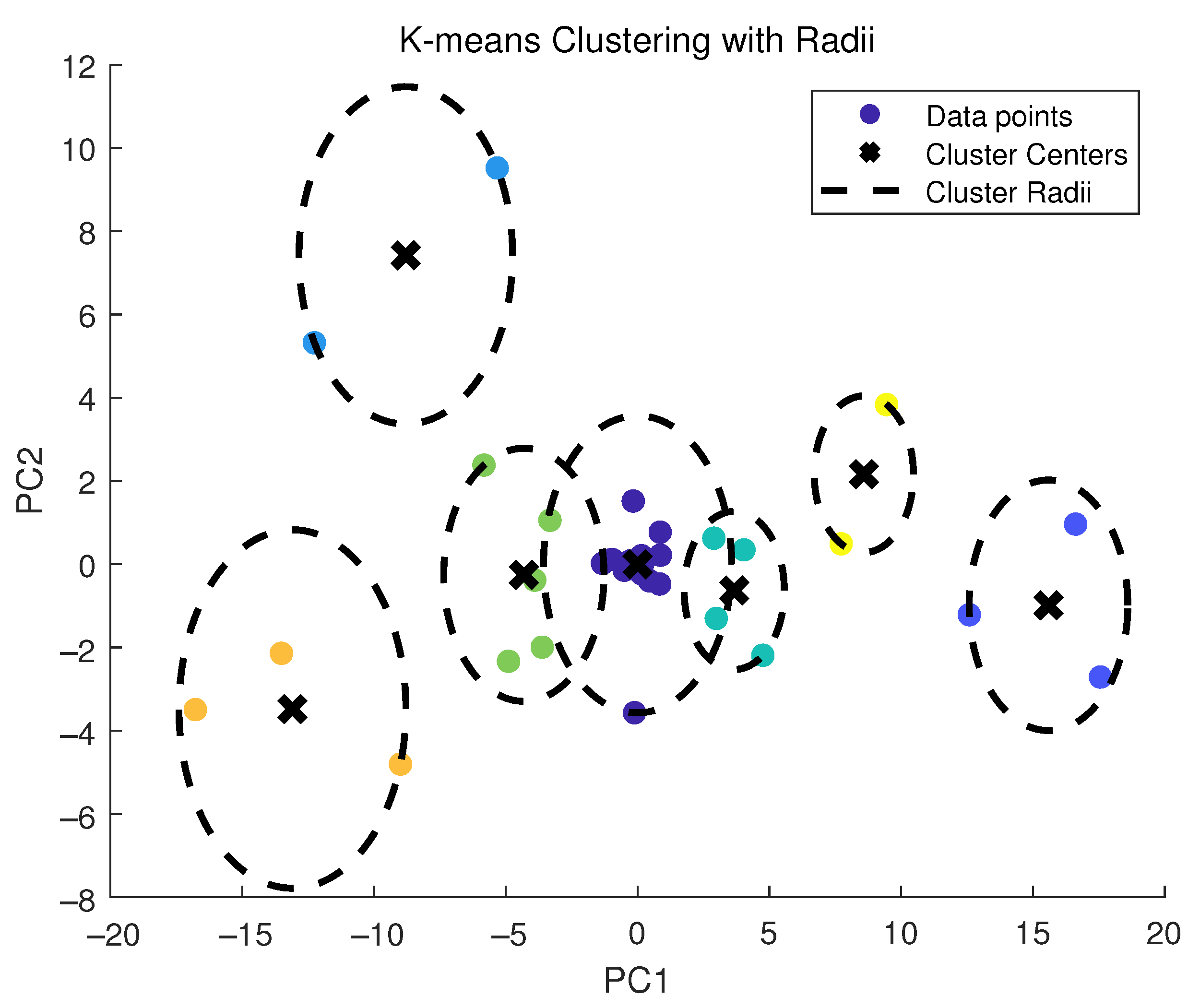
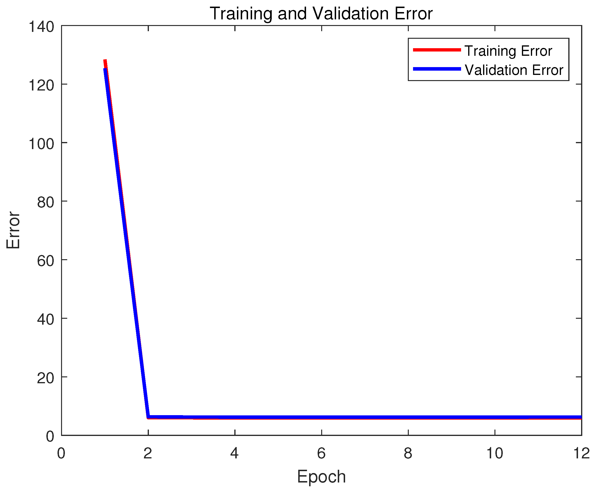
The control objective of the designed scheme is to ensure that the output belongs to one or more specific pattern classes, which distinguishes it from the previous model-free adaptive control. Initially, clustering and R B F neural networks classify a large number of outputs, obtained with valid control inputs, into several pattern classes. Then, one or more desired pattern classes are selected as the target for system control. In this case, 1000 uniformly distributed inputs are selected, and the corresponding outputs are obtained. The output is then normalized and then processed using PCA techniques to extract the principal component information set (the contribution rate: 88.8317% > 85%). The principal component information set is classified into pattern classes through clustering and neural networks. The classification method’s parameter settings are h = 7 , α = 0.1 , p = 0.01 (Figure 1: The I / O data curves of numerical example; Figure 2: The clustering results of numerical example. Different colors dots represent different classes; Figure 3: Tand validation error of numerical example; Table 1: The property values of pattern classes).
Remark 6.
As is well known, statistical pattern recognition includes various clustering and classification methods, such as ISODATA, K-means, and others. In this work, a combination of classification techniques of K-means and RBF neural network is used to classify the pattern class variable while training the neural network under the supervision of class results, trained with 700 datasets. It is then tested with 300 test sets to verify the accuracy of its pattern class variables classification. The classification accuracy of its model is 95%.
The dynamics of the system, based on pattern class variables, can be described as (47).
d x ( k + 1 ) = F p ( Φ ( k ) ) d x ¯ ( k + 1 ) = S ( d x ( k + 1 ) )
Seven pattern classes were derived, and the program designed was employed to track the following objectives:
d x ¯ * ( k + 1 ) = C ( 1 , 1 ) 0 < k 500 C ( 2 , 1 ) 500 < k 800 C ( mod ( k , h ) + 1 , 1 ) 800 < k 1000
where the first two tracked targets are represented as pattern classes 1 and 2, in which periodic updates are used to select the third tracked target, with the expectation d x ¯ * ( k + 1 ) takes this form.
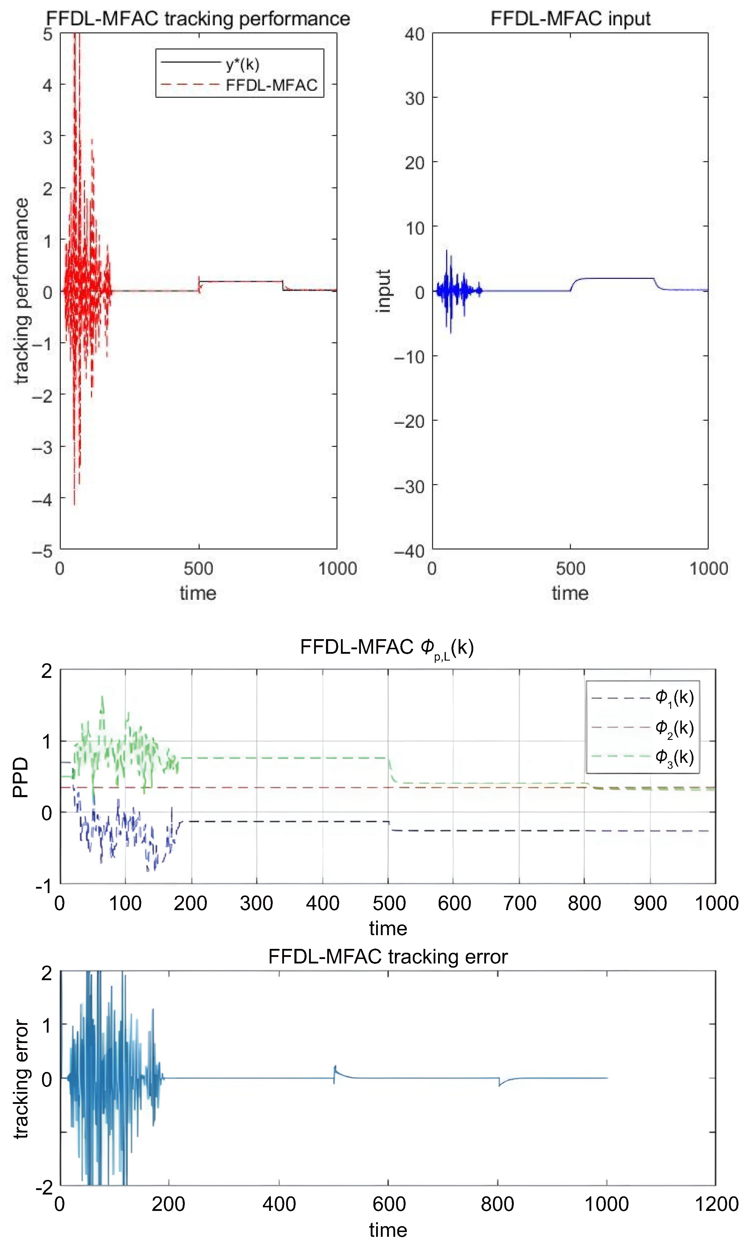
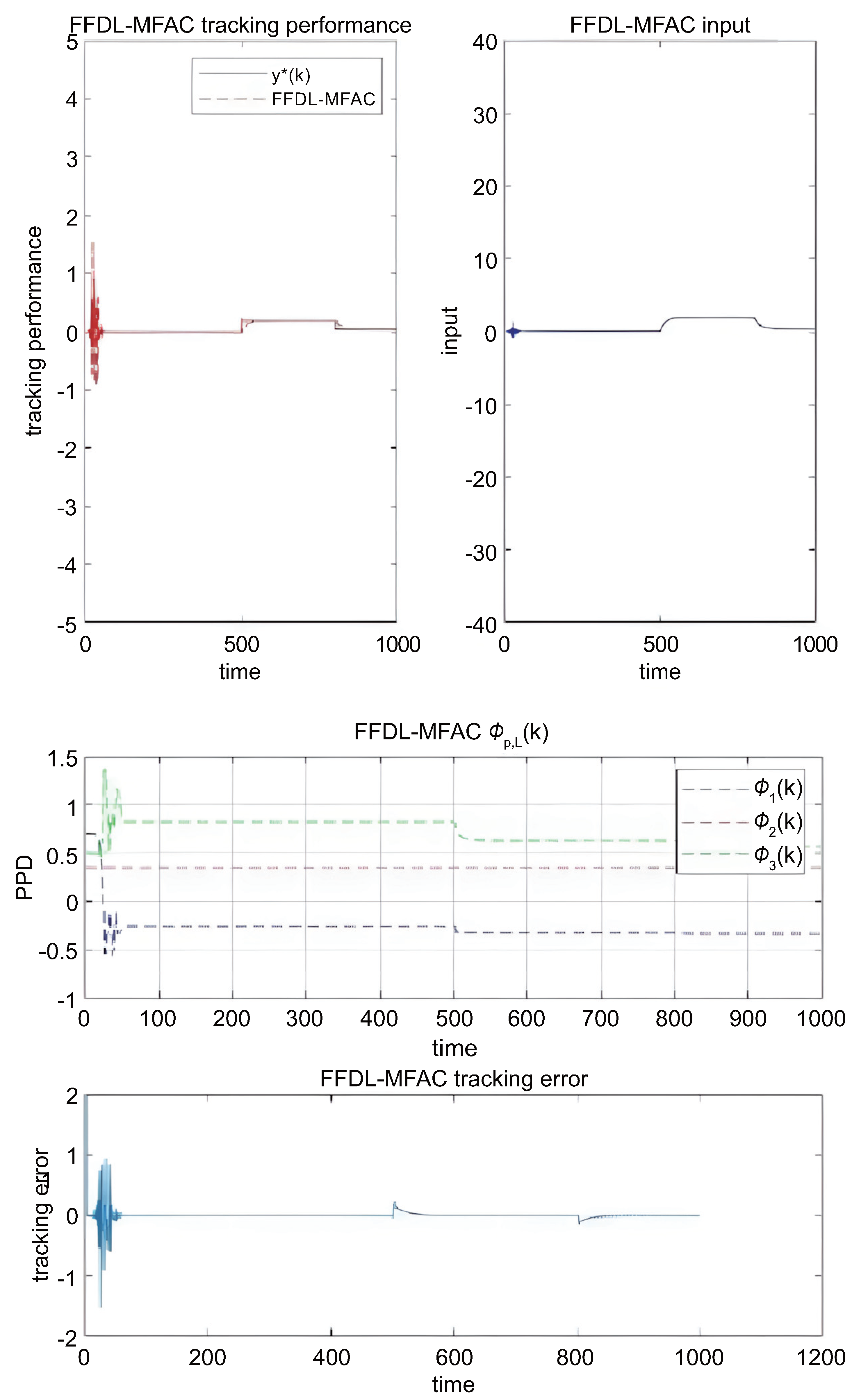
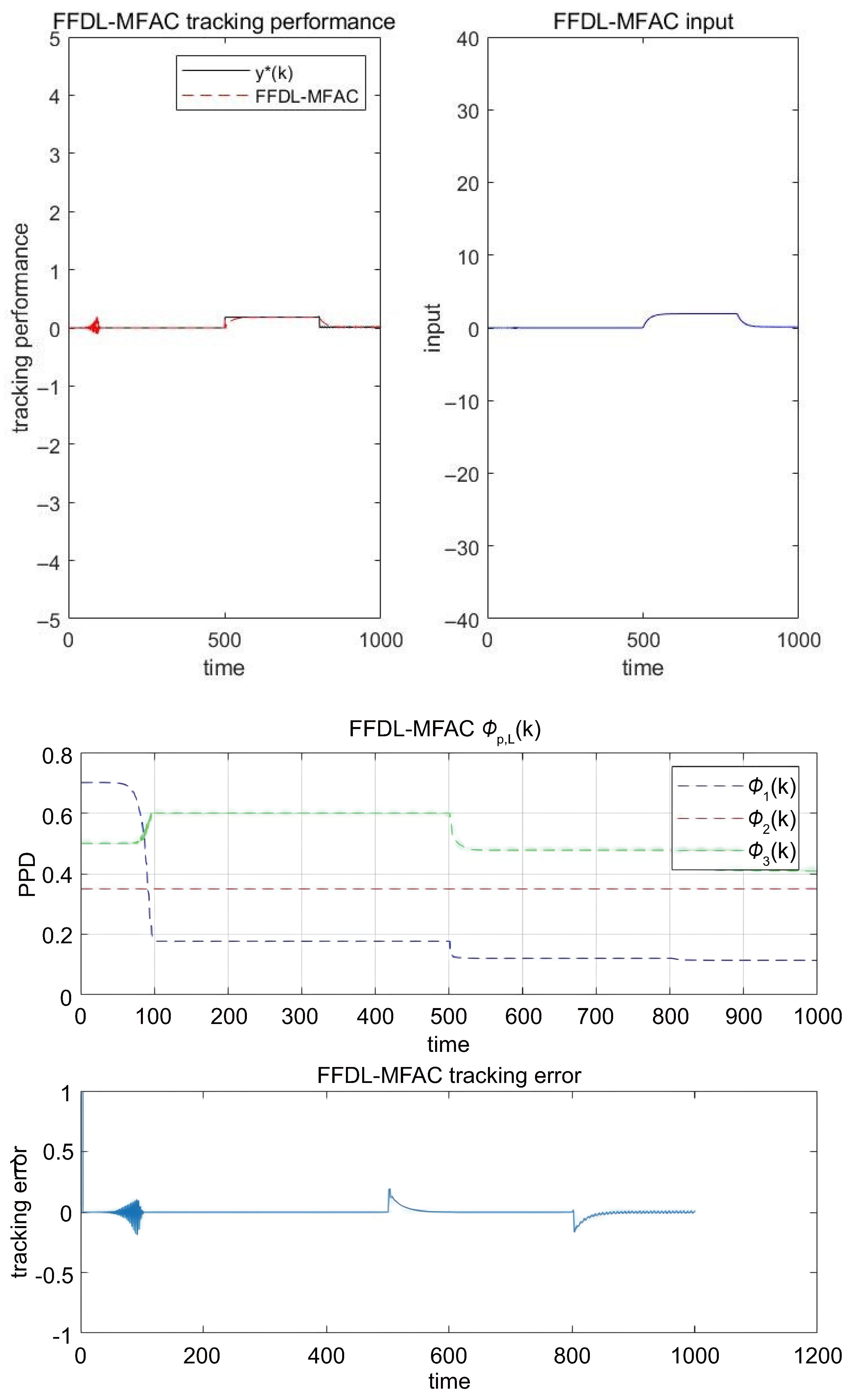
The initial condition is set to y ( 1 : 3 ) = 0 ; y ( 4 ) = 1 ; y ( 5 ) = 0 . 2 ; y ( 6 ) = 0 ;   u ( 1 : 6 ) = 0 ; u ( 5 ) = 0.5 ; the controller parameters are set to L u = 2 ; L y = 1 ; η = 1 ; μ = 1 ; λ = 0.01 ;   N = 1000 ;   Φ ^ L y , L u ( 1 ) = [ 0.7 , 0.35 , 0.5 ] T , Figure 4, Figure 5 and Figure 6 gives the P G estimation value, control input, estimated value, and tracking error, respectively, with ρ = 0.5 ,   ρ = 0.4 ,   ρ = 0.3 step factors, respectively. In Figure 4, Figure 5 and Figure 6, y * denotes the reference value. However, from these three figures, it can be seen that the tracking performance of ρ = 0.5 is poor and the tracking effect is poor, the tracking effect of ρ = 0.4 is slightly better, and the target trajectory of ρ = 0.3 is tracked well, and the tracking performance of the target trajectory has a better effect. The simulation results validate that the step factor value should align with the system’s complexity, and demonstrate that an appropriate step factor can enhance the system’s control performance. The numerical example illustrates that the proposed scheme is a highly practical method for a type of nonlinear discrete-time system. The simulation results show that for discrete-time nonlinear systems with unknown time-varying parameters, the scheme guarantees excellent output tracking performance of the closed-loop system.

5.2. Actual Example

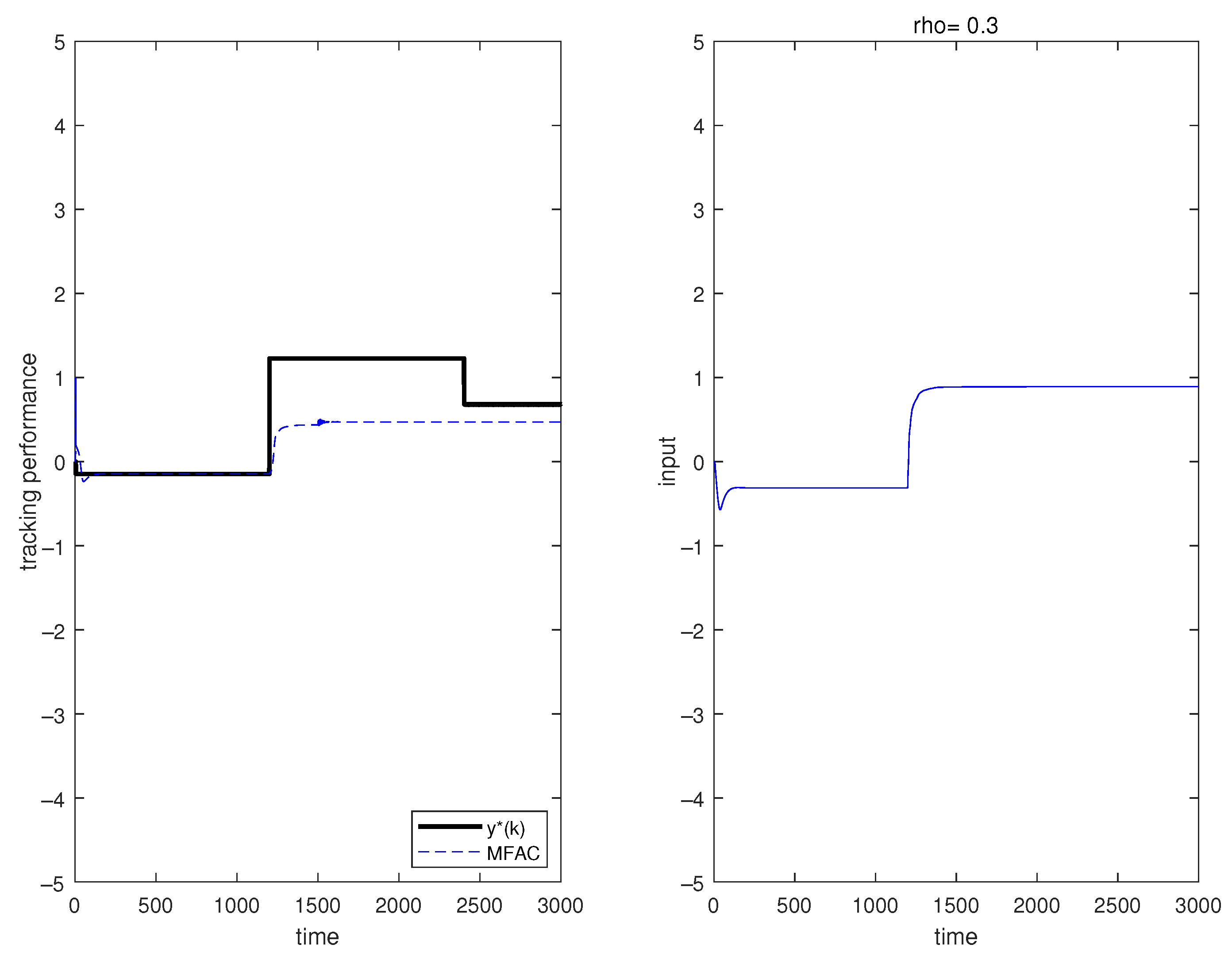
The proposed model-based model-free adaptive control system dynamics description method is simulated and verified using measured data collected from 400 sintering machine of Anyang Iron and Steel Co., Ltd (located in Anyang City, Henan Province, China). Many working conditions and operating data can be collected in the production process, such as temperature and pressure. However, since the end point of the sintering process is controlled at the penultimate bellows, the temperature of the three bellows at the end point is used as the output of the system, and the ignition temperature is used as the input of the system. There are 3000 sets of input and output data, the collected input and output data are normalized, and the output data are processed bytechnology, which changes the multidimensional output data into two-dimensional output data to obtain the principal component information set (principal component contribution rate: 86.5906% > 85%), and then the principal component information set is classified into different classes by this technology. In this study, the same classification technique approach was used as in Example 1, supervised by the clustering results and RBF, trained using 2100 datasets. It was then tested using 900 test sets (Figure 7: The clustering results of actual example; Figure 8: The clustering results of actual example. Different colors dots represent different classes; Figure 9: Training and validation error of actual example; Table 2: The property values of pattern classes).
The dynamics of the system, based on pattern class variables, can be described as (49).
d x ( k + 1 ) = F p ( Φ ( k ) ) d x ¯ ( k + 1 ) = S ( d x ( k + 1 ) )
Nine pattern classes were derived, and the program designed was employed to track the following objectives.
d x ¯ * ( k + 1 ) = C ( 4 , 1 ) 0 < k 1200 C ( 8 , 1 ) 1200 < k 2400 C ( mod ( k , h ) + 1 , 1 ) 2400 < k 3000
where the first two tracked targets are represented as pattern classes 4 and 8, and the selection of the third tracked target, expectation takes the form of periodic updates.
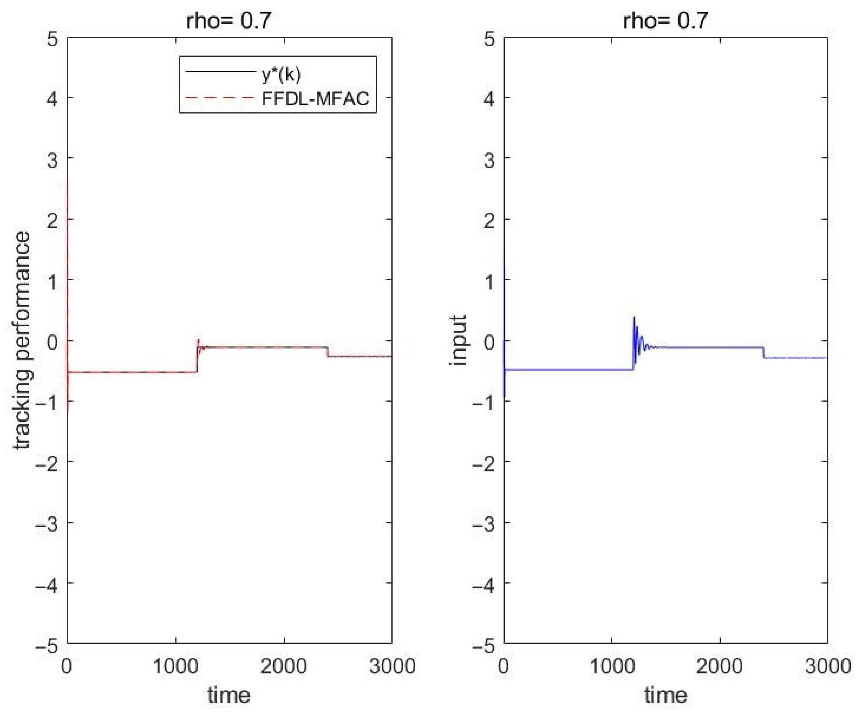
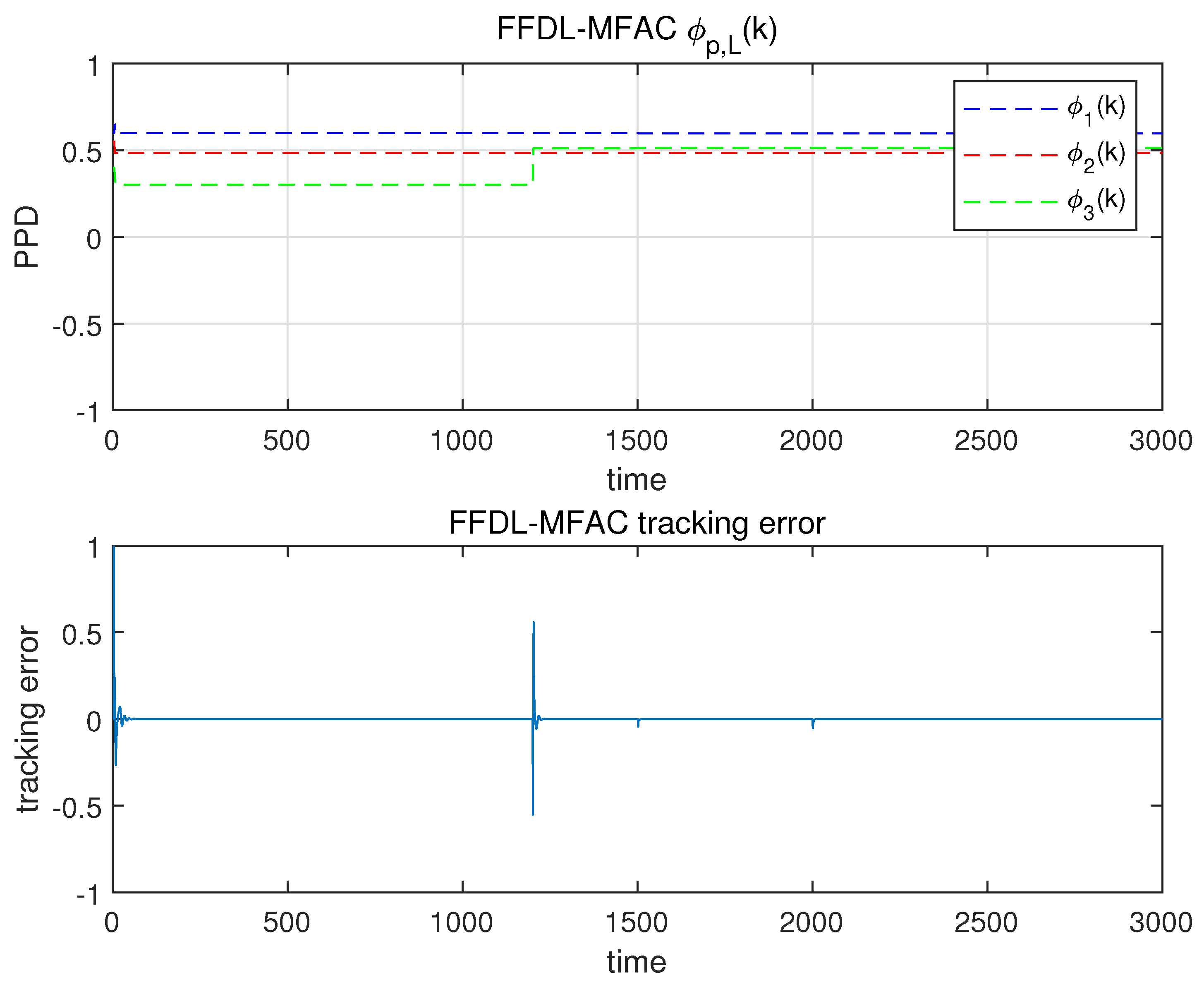
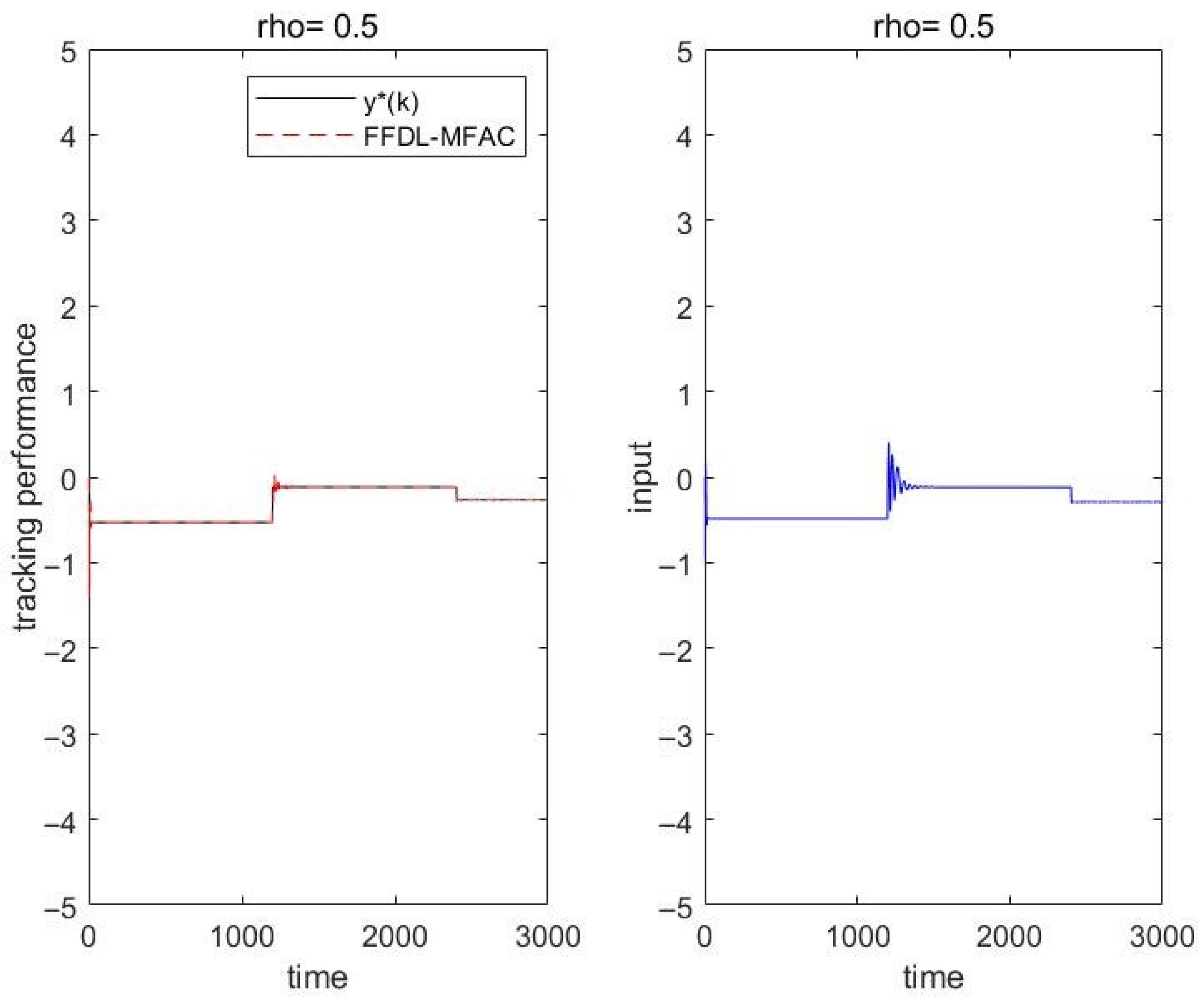
The initial condition is set to y ( 1 : 3 ) = 0 ; y ( 4 ) = 1 ; y ( 5 ) = 0 . 2 ; y ( 6 ) = 0 ;   u ( 1 : 6 ) = 0 ; u ( 5 ) = 0.5 ; the controller parameters are set to L u = 1 ; L y = 2 ; η = 1 ; μ = 1 ; λ = 0.001 ;   N = 3000 ;   Φ ^ L y , L u ( 1 ) = [ 0.6 , 0.55 , 0.4 ] T , Figure 10, Figure 11 and Figure 12 give the P G estimation value, control input, estimated value, and tracking error, respectively, with ρ = 0 . 5 ,   ρ = 0.4 ,   ρ = 0.3 step factors, respectively. In Figure 4, Figure 5 and Figure 6, y * denotes the reference value. The parameter settings of the adopted classification method are h = 9 ,   α = 0.001 ,   p = 0.05 . However, from these three figures, it can be seen that the tracking performance of ρ = 0.7 is poor and the tracking effect is poor, the tracking effect of ρ = 0.5 is slightly better, and the target trajectory of ρ = 0.3 is tracked well, and the tracking performance of the target trajectory has a better effect. The simulation results demonstrate that the tuning of the control parameters must be aligned with the system’s dynamics and show that proper tuning significantly enhances system performance.
The numerical example illustrates that the proposed approach is highly effective for a particular class variable of nonlinear continuous-time systems, where the goal is to control the output to specific desired states or ranges. The system’s output is dynamically adjusted without the need for an explicit model, comparisons with the target output, ensuring the desired performance even in the absence of a known system model. From the simulation outcomes, it is evident that for continuous-time nonlinear systems with unknown time-varying parameters, the proposed scheme guarantees robust tracking performance of system variables under various operational conditions.
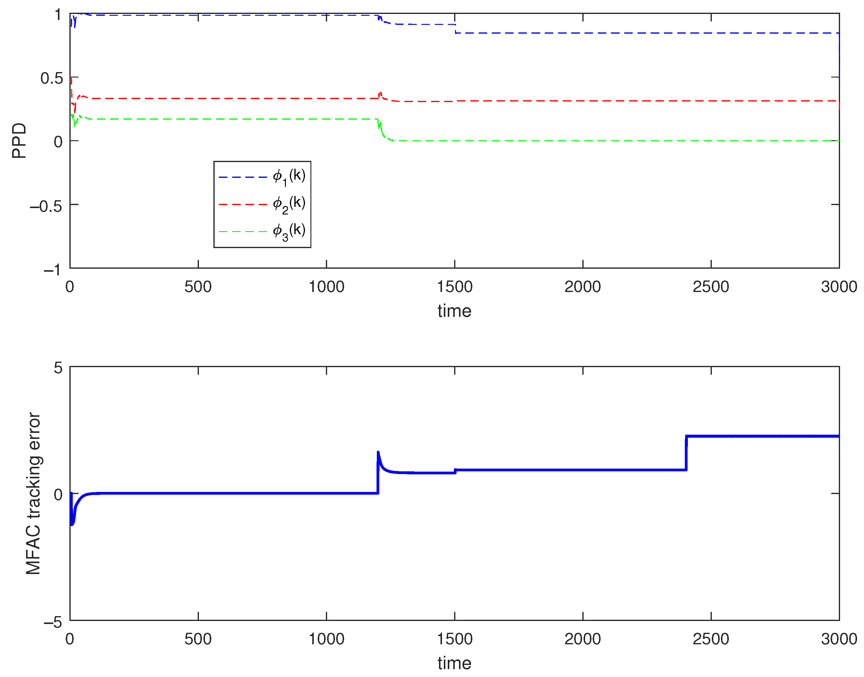
In order to verify the effectiveness of the proposed method, it is compared with the traditional MFAC method. The comparison results are shown in Figure 13. The P-FFDL-MFAC tracking error is 0.068, and the MFAC tracking error is 1.178. The results show that the proposed method is superior to the traditional MFAC method.

6. Conclusions

This study addresses the problem of model-free adaptive control for systems with nonlinear time-varying dynamic properties. In the design process, the input-output relationship, pattern class variables, and the robustness of the system are considered. Based on a combination of principal component analysis (PCA) dimensionality reduction, K-means clustering, and neural network training, a model-free adaptive control strategy is used to achieve the desired output pattern class. The method aims to minimize the tracking error while ensuring robust performance under output perturbations and system uncertainties. In order to verify the effectiveness of the proposed control scheme, its performance is evaluated through a series of experiments for different values of system parameters. The simulation results clearly show that the designed model-free adaptive control strategy performs well in handling output perturbations and ensures the robustness of the control system. However, it can be seen from the simulation results that the control method proposed in this paper has good performance. But it should also include the ability to deal with data dropout, which may be caused by sensor faults, transmission network failures, or actuator damage. Therefore, the next topic that needs to be focused on is the robustness of pattern moving-based model-free adaptive control on faults.

Author Contributions

Conceptualization, J.W. and M.H.; methodology, J.W.; software, M.H.; validation, J.W. and M.H.; formal analysis, M.H.; investigation, M.H.; resources, J.W.; data curation, M.H.; writing—original draft preparation, M.H.; writing—review and editing, M.H.; visualization, J.W.; supervision, J.W.; project administration, J.W.; funding acquisition, J.W. All authors have read and agreed to the published version of the manuscript.

Funding

This research was funded by the Natural Science Project of Liaoning Provincial Department of Science and Technology (No. 2024-MS-190), General Project of Liaoning Provincial Department of Education of China (No. JYTMS20230868), and the National Natural Science Foundation of China (No. 61903167).

Data Availability Statement

The data that support the findings of this study are available on request from the corresponding author. The data are not publicly available due to privacy or ethical restrictions.

Conflicts of Interest

The authors declare no conflicts of interest.

References

  1. Sklansky, J. Learning systems for automatic control. IEEE Trans. Autom. Control 1996, 11, 6–19. [Google Scholar] [CrossRef]
  2. Yin, S.; Gao, H.; Kaynak, O. Data-driven control and process monitoring for industrial applications—Part I. IEEE Trans. Ind. Electron. 2014, 61, 6356–6359. [Google Scholar] [CrossRef]
  3. Xu, Z. A pattern recognition approach to model a class of complex systems. J. Comput. Inf. Syst. 2011, 7, 4636–4643. [Google Scholar]
  4. Qu, S.D. Pattern recognition approach to intelligent automation for complex industrial processes. J. Univ. Sci. Technol. Beijing 1998, 20, 385–389. [Google Scholar] [CrossRef]
  5. Saridis, G.N. Application of pattern recognition method to control systems. IEEE Trans. Autom. Control 1981, 26, 638–645. [Google Scholar] [CrossRef]
  6. Zhu, Q.; Onori, S.; Prucka, R. Pattern recognition technique based active set QP strategy applied to MPC for a driving cycle test. IEEE Am. Control Conf. 2015, 7, 4935–4940. [Google Scholar] [CrossRef]
  7. Yu, B.; Zhang, X.; Wu, L.; Chen, X. A novel postprocessing method for robust myoelectric pattern-recognition control through movement pattern transition detection. IEEE Trans. Hum.-Mach. Syst. 2020, 50, 32–41. [Google Scholar] [CrossRef]
  8. Xu, Z. Pattern Recognition Method of Intelligent Automation and Its Implementation in Engineering. Doctoral Dissertation, University of Science and Technology Beijing, Beijing, China, 2001. [Google Scholar]
  9. Wang, M.; Xu, Z.; Guo, L. Stability and stabilization for a class of complex production processes via LMIs. Optim. Control Appl. Methods 2019, 40, 460–478. [Google Scholar] [CrossRef]
  10. Sun, C.; Xu, Z.; Guo, L. Multi-dimensional moving pattern prediction based on multi-dimensional interval T-S fuzzy model. J. Control Decis. 2016, 31, 1569–1576. [Google Scholar]
  11. Hai, P.P.; Xia, C. Global robust optimal sliding mode control for uncertain affine nonlinear systems. J. Syst. Eng. Electron. 2009, 20, 838–843. [Google Scholar]
  12. Yu, S.; Guo, G.; Ma, Z. Global fast terminal sliding mode control for robotic manipulators. Int. J. Model. Identif. Control 2006, 1, 72–79. [Google Scholar] [CrossRef]
  13. Skruch, P. A terminal sliding mode control of disturbed nonlinear second-order dynamical systems. J. Comput. Nonlinear Dyn. 2016, 11, 054501. [Google Scholar] [CrossRef]
  14. Tayebi-Haghighi, S.; Piltan, F.; Kim, J.M. Robust composite high-order super-twisting sliding mode control of robot manipulators. Robotics 2018, 7, 13. [Google Scholar] [CrossRef]
  15. Guo, L.; Xu, Z.; Wang, Y. Dynamic modeling and optimal control for complex systems with statistical trajectory. Discret. Dyn. Nat. Soc. 2015, 2015, 245685. [Google Scholar] [CrossRef]
  16. Piltan, F.; TayebiHaghighi, S.; Sulaiman, N.B. Comparative study between ARX and ARMAX system identification. J. Int. J. Intell. Syst. Appl. 2017, 9, 25–34. [Google Scholar] [CrossRef]
  17. Kon, J.; Yamashita, Y.; Tanaka, T.; Tashiro, A.; Daiguji, M. Practical application of model identification based on ARX models with transfer functions. Control Eng. Pract. 2013, 21, 195–203. [Google Scholar] [CrossRef]
  18. Mobayen, S.; Tchier, F. A novel robust adaptive second-order sliding mode tracking control technique for uncertain dynamical systems with matched and unmatched disturbances. Int. Control Autom. Sust. 2017, 15, 1097–1106. [Google Scholar] [CrossRef]
  19. Yeh, Y.L. A Robust Noise-Free Linear Control Design for Robot Manipulator with Uncertain System Parameters. J. Actuators 2021, 10, 121. [Google Scholar] [CrossRef]
  20. Lee, J.H.; Lee, K.S. Iterative learning control applied to batch processes: An overview. J. Control Eng. Pract. 2007, 15, 1306–1318. [Google Scholar] [CrossRef]
  21. Jiang, H.; Zhang, H.; Liu, Y. Neural-network-based control scheme for a class of nonlinear systems with actuator faults via data-driven reinforcement learning method. J. Neurocomput. 2017, 239, 1–8. [Google Scholar] [CrossRef]
  22. Ahn, H.; Chen, Y.; Moore, K. Iterative learning control: Brief survey and categorization. IEEE Trans. Syst. Man. Cybern. Part C Appl. Rev. 2007, 37, 1099–1121. [Google Scholar] [CrossRef]
  23. Pierallini, M.; Angelini, F.; Mengacci, R. Iterative learning control for compliant underactuated arms. IEEE Trans. Syst. Man Cybern. Syst. 2023, 53, 3810–3822. [Google Scholar] [CrossRef]
  24. Zhou, M.; Li, T.; Zhang, C. Sliding mode iterative learning control with iteration-dependent parameter learning mechanism for nonlinear systems and its application. IEEE Trans. Autom. Sci. Eng. 2023, 21, 7052–7063. [Google Scholar] [CrossRef]
  25. Xu, Z.; Wu, J.; Guo, L. Modeling and optimal control based on moving pattern. In Proceedings of the 32nd Chinese Control Conference, Xi’an, China, 26–28 July 2013; pp. 7894–7899. Available online: https://ieeexplore.ieee.org/document/6640830 (accessed on 1 March 2024).
  26. Bu, X.H.; Hou, Z.S.; Zhang, H.W. Data driven multiagent systems consensus tracking using model free adaptive control. IEEE Trans. Neural Netw. Learn. Syst. 2018, 29, 1514–1524. [Google Scholar] [CrossRef]
  27. Li, X.Q.; Xu, Z.G.; Lu, Y.L.; Cui, J.R.; Zhang, L.X. Modified Model Free Adaptive Control for a Class of Nonlinear Systems with Multi-threshold Quantized Observations. Int. J. Control. Autom. Syst. 2021, 19, 3285–3296. [Google Scholar] [CrossRef]
  28. Xu, Z.; Wu, J. Data-driven pattern moving and generalized predictive control. In Proceedings of the 2012 lEEE Interational Conference on Systems, Man and Cybernetics, Seoul, Republic of Korea, 14–17 October 2012. [Google Scholar] [CrossRef]
  29. Hou, Z.S.; Xiong, S.S. On model-free adaptive control and its stability analysis. IEEE Trans. Autom. Control 2019, 11, 4555–4569. [Google Scholar] [CrossRef]
  30. Hou, Z.S.; Jin, S.T. Model Free Adaptive Control: Theory and Applications; CRC Press: Boca Raton, FL, USA, 2013. [Google Scholar] [CrossRef]
  31. Li, X.Q.; Xu, Z. Pattern-Moving-Based Partial Form Dynamic Linearization Model Free Adaptive Control for a Class of Nonlinear Systems. J. Actuators 2021, 10, 223. [Google Scholar] [CrossRef]
  32. Basohbat Novinzadeh, A.; Heydari, M.; Yaseri, M. Model-Free Adaptive Controller Design for Nonlinear system of an Air Vehicle pitch channel. Modares Mech. Eng. 2018, 17, 161–171. [Google Scholar]
  33. Gao, H.; Ma, G.; Lv, Y. Forecasting-based data-driven model-free adaptive sliding mode attitude control of combined spacecraft. J. Aerosp. Sci. Technol. 2019, 86, 364–374. [Google Scholar] [CrossRef]
  34. Qiu, X.; Wang, Y.; Xie, X.; Zhang, H. Resilient model-free adaptive control for cyber-physical systems against jamming attack. J. Neurocomput. 2020, 413, 422–430. [Google Scholar] [CrossRef]
  35. Yongjun, D.; Jianhong, W.; Jinlong, Z.; Xi, L. Design of quadcopter attitude controller based on data-driven model-free adaptive sliding mode control. Int. J. Dyn. Control 2024, 12, 1404–1414. [Google Scholar] [CrossRef]
  36. Ren, C.; Jiang, H.; Li, C.; Sun, W.; Ma, S. Koopman-operator-based robust data-driven control for wheeled mobile robots. IEEE/ASME Trans. Mech. 2022, 28, 461–472. [Google Scholar] [CrossRef]
  37. Bu, X.; Dai, X.; Hou, R. Data-driven iterative learning trajectory-tracking control for wheeled mobile robot under constraint of velocity saturation. IET Cyber-Syst. Robot. 2023, 5, e12091. [Google Scholar] [CrossRef]
  38. Hou, R.; Cui, L.; Bu, X.; Yang, J. Distributed formation control for multiple non-holonomic wheeled mobile robots with velocity constraint by using improved data-driven iterative learning. Appl. Math. Comput. 2021, 395, 125829. [Google Scholar] [CrossRef]
  39. Huang, J.; Chen, H.; Shen, C. Event-Triggered Model-Free Adaptive Control for Wheeled Mobile Robot with Time Delay and External Disturbance Based On Discrete-Time Extended State Observer. J. Dyn. Syst. Meas. Control 2024, 146, 021005. [Google Scholar] [CrossRef]
  40. Tutsoy, O.; Barkana, D.E. Model free adaptive control of the under-actuated robot manipulator with the chaotic dynamics. J. ISA Trans. 2021, 118, 106–115. [Google Scholar] [CrossRef] [PubMed]
  41. Earl, R.; Nicholson, J. The Concise Oxford Dictionary of Mathematics, 6th ed.; Oxford University Press: Oxford, UK, 2021. [Google Scholar] [CrossRef]
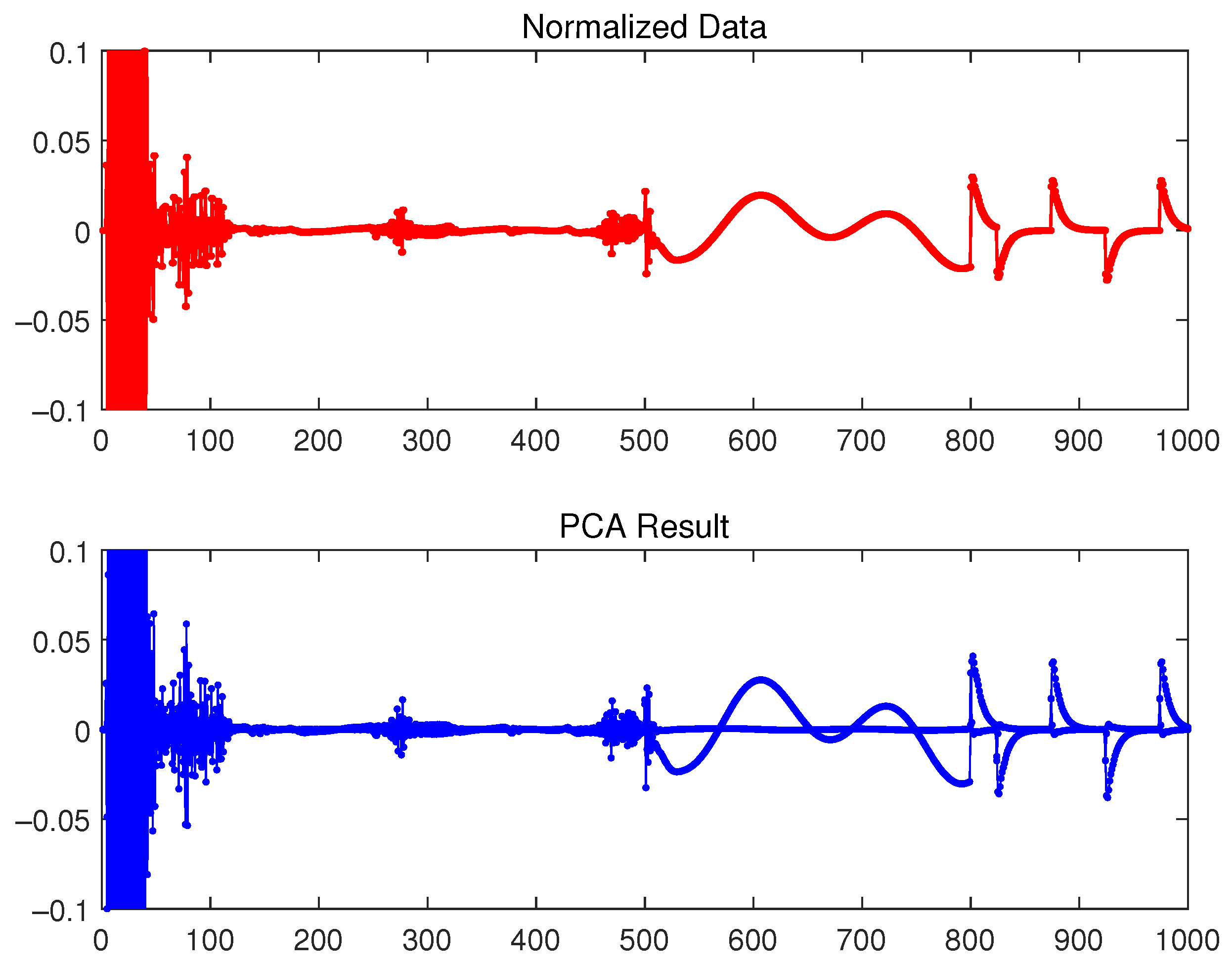
Figure 1. The I / O data curves of numerical example.
Mathematics 13 02717 g001
Figure 2. The clustering results of numerical example.
Mathematics 13 02717 g002
Figure 3. Trainingand validation error of numerical example.
Mathematics 13 02717 g003
Figure 4. The PG estimation value, control input, error, and tracking performance curves with ρ = 0.5 .
Mathematics 13 02717 g004
Figure 5. The PG estimation value, control input, error, and tracking performance curves with ρ = 0.4 .
Mathematics 13 02717 g005
Figure 6. The PG estimation value, control input, error, and tracking performance curves with ρ = 0.3 .
Mathematics 13 02717 g006
Figure 7. The clustering results of actual example.
Mathematics 13 02717 g007
Figure 8. The class centers of actual example.
Mathematics 13 02717 g008
Figure 9. Training and validation error of actual example.
Mathematics 13 02717 g009
Figure 10. The PG estimation value, control input, error, and tracking performance curves with ρ = 0.7 .
Mathematics 13 02717 g010aMathematics 13 02717 g010b
Figure 11. The PG estimation value, control input, error, and tracking performance curves with ρ = 0.5 .
Mathematics 13 02717 g011aMathematics 13 02717 g011b
Figure 12. The PG estimation value, control input, error, and tracking performance curves with ρ = 0.3 .
Mathematics 13 02717 g012aMathematics 13 02717 g012b
Figure 13. The MFAC PG estimation value, control input, error, and tracking performance curves with ρ = 0.3 .
Mathematics 13 02717 g013aMathematics 13 02717 g013b
Table 1. The property values of pattern classes.
Class No.Class CenterClass Radius
1(−0.0180, −0.0073)2.9853
2(7.3567, 6.2062)5.5453
3(−13.0390, −0.8266)1.5866
4(0.1367, 1.2690)1.1211
5(10.9540, −2.9166)2.4866
6(−7.1804, 1.8080)2.8153
7(3.6094, −0.2141)2.5436
Table 2. The property values of pattern class variables.
Class No.Class CenterClass Radius
1(−0.5017, −0.5580)0.4961
2(0.1857, 0.6282)0.4600
3(1.8278, −0.4929)0.4331
4(−2.9019, −0.7778)0.6773
5(−1.7517, 0.1289)0.4487
6( 0.6954, −0.4751)0.4388
7(1.4996, 0.5842)0.5166
8(−0.8493, 0.4924)0.3953
9(3.0346, 0.2092)0.6028
Disclaimer/Publisher’s Note: The statements, opinions and data contained in all publications are solely those of the individual author(s) and contributor(s) and not of MDPI and/or the editor(s). MDPI and/or the editor(s) disclaim responsibility for any injury to people or property resulting from any ideas, methods, instructions or products referred to in the content.