Article

A Novel Consistency Index CI-G: Recruiting Compatibility Index G for Consistency Analysis

1
Fulcrum Ingeniería Ltd., Santiago 0180, Chile
2
Department of Business Management, Accounting and Ethics, Carlow University, Pittsburgh, PA 15213, USA
*
Author to whom correspondence should be addressed.
Mathematics 2025, 13(16), 2666; https://doi.org/10.3390/math13162666
Submission received: 26 May 2025 / Revised: 4 August 2025 / Accepted: 15 August 2025 / Published: 19 August 2025

Abstract

Consistency indices quantify the degree of transitivity and proportionality violations in a pairwise comparison matrix (PCM), forming a cornerstone of the Analytic Hierarchy Process (AHP) and Analytic Network Process (ANP). Several methods have been proposed to compute consistency, including those based on the maximum eigenvalue, dot product, Jaccard index, and the Bose index. However, these methods often overlook two critical aspects: (i) vector projection or directional alignment, and (ii) the weight or importance of individual elements within a pointwise evaluative structure. The first limitation is particularly impactful. Adjustments made during the consistency improvement process affect the final priority vector disproportionately when heavily weighted elements are involved. Although consistency may improve numerically through such adjustments, the resulting priority vector can deviate significantly, especially when the true vector is known. This indicates that approaches neglecting projection and weighting considerations may yield internally consistent yet externally incompatible vectors, thereby compromising the validity of the analysis. This study builds on the idea that consistency and compatibility are intrinsically related; they are two sides of the same coin and should be considered complementary. To address these limitations, it introduces a novel metric, the Consistency Index G (CI-G) based on the compatibility index G. This measure evaluates how well the columns of a PCM align with its principal eigenvector, using CI-G as a diagnostic component. The proposed approach not only refines consistency measurement but also enhances the accuracy and reliability of derived priorities.

1. Introduction

The Analytic Hierarchy Process (AHP) and its generalization, the Analytic Network Process (ANP), are well-known and widely disseminated methodologies worldwide due to a combination of mathematical rigor and simplicity of use [1]. AHP/ANP methodology requires that the decision-maker(s) perform a pairwise comparison of elements in the pairwise comparison matrix (PCM) (e.g., criteria, alternatives) to obtain their relative priorities (e.g., importance, preference), also called the priority vector [2]. Two concepts directly related to AHP/ANP methodology are PCM consistency and compatibility between two priority vectors.
Consistency refers to the degree to which each direct comparison aik in a PCM is fully supported by the corresponding set of indirect comparisons aij × ajk  j . A matrix is deemed consistent when this condition of multiplicative transitivity is satisfied across all entries. In essence, a decision-maker who provides fully consistent judgments ensures that no internal contradictions exist among the stated preferences [3]. Saaty [4] introduced a consistency index (CI) that was later re-scaled as a consistency ratio, CR = CI/RI, where RI corresponds to the consistency index of a random matrix of the same order as the PCM being evaluated. While this consistency index CR has traditionally been used by AHP/ANP practitioners, other consistency indices have been introduced such as the geometric index GCI introduced by Crawford [5] and further developed [6]. A generalization of the GCI approach has been recently proposed [7]. More inconsistency indices and approaches have been proposed such as the consistency index CI* [8,9], the linearization technique to obtain the nearest consistent matrix corresponding to a given inconsistent matrix [10,11], and a new definition of consistency [12,13]. Others have been developed and are discussed in the extant literature, such as Pant, et al. [14].
Compatibility, within the context of the AHP/ANP, refers to the degree of closeness or similarity between two vectors, indicating the extent to which they can be considered compatible [15]. Compatibility analysis is frequently applied in group decision-making scenarios, where individual participants construct their own pairwise comparison matrices (PCMs) and corresponding priority vectors, necessitating comparison to evaluate the degree of alignment [16,17]. It is also commonly employed in predictive modeling, where the predicted priority vector is assessed against a known or “true” priority vector to evaluate its accuracy [18,19]. The first formal metric for compatibility was Saaty’s compatibility index S, which is based on the Hadamard product and has been extensively utilized in the literature. An alternative measure, the consistency index G, was later introduced by Garuti [20] and has proven particularly effective for evaluating compatibility with respect to a known priority vector [21].
The present study posits that consistency and compatibility represent two sides of the same coin. In the context of a PCM, consistency is conceptualized as an internal or reflexive property, as it is assessed solely with reference to the matrix itself, particularly its principal eigenvector. By contrast, compatibility is treated as an external property, as it involves comparing the priority vector derived from a given PCM to an external priority vector obtained from a different PCM [22]. This distinction builds upon Saaty’s discussion of consistency and compatibility, wherein consistency is defined as the “compatibility of a matrix of the ratios constructed from a principal right eigenvector with the matrix of judgments from which it is derived” [23].
Given this distinction, it follows that consistency can be interpreted as a compatibility issue. That is, consistency can be assessed by leveraging compatibility. To this end, this study introduces CI-G (Consistency Index G) as a novel approach to measuring consistency through compatibility and demonstrates the advantages of this method. Thus, this research proposes a paradigm shift in consistency measurement, redefining it in terms of compatibility, as will be further elaborated in the following sections. This study aims to demonstrate that the proposed CI-G provides enhanced reliability and interpretive clarity relative to existing consistency measures. The advantages of CI-G are discussed in the following.
The CI-G threshold is defined as an absolute value, independent of external factors such as matrix size or input data. This enables broader applicability across a wide range of decision-making contexts. Also, and more importantly, it accounts for the weights and projections of the priority vector, thereby refining the consistency measurement and enhancing both the accuracy and reliability of the derived priorities. Additionally, it provides clearer indications of where to intervene to improve the consistency of the PCM.
In summary, as elaborated in this study, the proposed method is grounded in the compatibility G index, which itself is based on order topology. This index captures the intensity of preferences through point-to-point vector alignment (vector projection), which is mathematically rooted in the weighted cosine similarity function. This cardinal index introduces a novel and distinctive approach by simultaneously incorporating both weight and vector projection for every coordinate (point) of the priority vector, thereby offering a unique measure of consistency.

2. Theoretical Framework

Next, we will perform a brief review of the theoretical concepts related to the discussion of the proposed consistency index.

2.1. The Compatibility Index G

The compatibility index G, introduced by Garuti [22], has been widely employed to compare priority vectors in multi-criteria decision-making (MCDM) analysis, as well as in other domains when the need arises to quantitatively compare the congruence of two multidimensional constructs [24,25]. The popularity of the compatibility index G stems from its geometric interpretability and computational simplicity. However, it’s most significant advantage lies in its precision in measuring compatibility, as it accounts for the projection and, at the same time, the relevance of elements that constitute both priority vectors. In this framework, the numerical values in each vector are not merely figures but represent the importance of the criteria as weighted components.
A key distinguishing feature of the compatibility index G is its point-to-point weighting of the angular difference between vectors across the entire priority vector, which can also be interpreted as a behavioral profile. This methodology is based on the premise that compatibility in a heavily weighted PCM element carries more significance than in a lightly weighted one. In its calculation, the compatibility index G simultaneously considers both the weight and angular projection of each coordinate when measuring compatibility between vectors. Similarly, when comparing behavioral profiles, it integrates the weight and projection of each profile point. Notably, the compatibility index G can be regarded as a mathematical generalization of the Jaccard index (J) [26].
Given these properties, investigating the derivation of a consistency measure based on the compatibility index G formulation is a critical research question. This study, therefore, proposes the CI-G as a novel approach to measuring consistency through compatibility in the AHP/ANP, thereby advancing the evaluation quality of pairwise comparison matrices (PCMs).

2.1.1. Overview

Compatibility index G is a transformation function that operates on positive real numbers within the range [0, 1], derived from normalized vectors A and B. It outputs a positive real number within the same range [0, 1], representing the degree of compatibility between A and B, where 0 indicates no compatibility and 1 indicates full compatibility (i.e., 0% to 100%). The demonstration given in Equation (1) is based on the original development of the compatibility index G; a brief explanation of this equation is provided in Appendix B for the reader’s convenience [20,22].
The function G is defined as follows:
G = 1 2 i = 1 , n a ( i ) + b ( i )   M i n a ( i ) , b ( i ) M a x a ( i ) , b ( i )
where a(i) and b(i) denotes elements of the priority vectors A and B, respectively.
If the AHP/ANP model is a rating model (i.e., in absolute measurement mode), the preceding equation is reduced to:
G = i = 1 , n w ( i ) M i n a ( i ) , b ( i ) M a x a ( i ) , b ( i )
where w(i) denotes the vector of weights derived from the set of global weights associated with the terminal criteria; a, b represents the ratings assigned across the scales of each terminal criterion for the performance profiles of alternatives A and B, respectively.

2.1.2. Properties

Compatibility index G is a transformation that adheres to the three metric properties of a distance function, which are reflexivity, identity of indiscernible (zero property) and triangle inequality [27]. The compatibility index G ranges from 0 to 1, thereby avoiding any divergence issues. Values exceeding 1 are difficult to interpret, as it is unclear what it would mean to be more than 100% compatible. Additionally, G possesses a fourth property: non-transitivity of compatibilities. Specifically, if vector A is compatible with vector B, and B is compatible with vector C, it does not necessarily follow that A is compatible with C; compatibility may or may not hold in this case. This non-transitive property can, in certain contexts, be particularly useful. For example, consider two identical eigenvectors derived from two distinct PCMs: an initial PCM and a perturbed version. If the initial PCM is fully compatible with its eigenvector—meaning all of its columns are proportional to the eigenvector, thereby rendering the matrix fully consistent—and this eigenvector is also fully compatible with that of the perturbed PCM (i.e., both matrices share the same eigenvector), it does not necessarily follow that the columns of the perturbed PCM must be compatible with those of the initial PCM. Consequently, the perturbed PCM may or may not be consistent. In other words, the mere fact that the initial and perturbed PCMs have the same eigenvector, and that the initial PCM is consistent, does not imply that the perturbed PCM must also be consistent. This point is revisited in a subsequent section.

2.2. Scales, Homogeneity and Consistency

Consistency is closely related to the principles of proportionality and transitivity in PCMs. Specifically, the condition of proportionality is as follows:
a(i,k) × a(k,j) = a(i,j)
If Equation (3) holds for all i, j, and k, the PCM is fully consistent. However, if it deviates, such as the following:
a(i,k) × a(k,j) > a(i,j)
then proportionality is lost, though transitivity may still hold. If Equation (4) is iteratively raised to increasing powers (e.g., 2, 3, 4, …), consistency will deteriorate significantly. This principle underlies newly proposed Axiom 3—monotonicity under reciprocity-preserving mapping [28]—which requires that comparison scales be extendable as needed. Consequently, the matrix dimension (n) becomes a key factor in defining the consistency threshold, regardless of the scale (e.g., 1–9, 1–100, exponential scales). Notably, Saaty [29] emphasized that his consistency ratio index (CR) remains unaffected regardless of the scale employed in a PCM.
In principle, CI-G fails to meet Axiom 3. If a PCM is exponentiated sufficiently, CI-G approaches zero, giving a wrong result for consistency. However, this raises a critical question; is it more important to allow arbitrary scale extension or to ensure good consistency within cognitively feasible human scales? To address this, recall that Saaty’s fundamental scale (1–9) reflects human limitations. Humans struggle to compare elements differing by more than one order of magnitude, compromising both proportionality and transitivity. In fact, Saaty’s fundamental scale is based on Miller [30]’s findings on human information processing constraints. This limitation justifies Saaty’s [29] AHP/ANP Axiom 2, which asserts that elements of vastly different magnitudes should not be directly compared; for example, comparing an elephant to an ant would violate this principle.
This article argues that strict adherence to Axiom 2, including the use of Saaty’s 1–9 scale, renders Axiom 3 [28,31] largely redundant in the AHP/ANP framework. Beyond supporting consistency, Axiom 2 prevents poorly structured models. Ensuring logical model structure is a prerequisite for meaningful consistency. Consider elements A, B, and C with A = 6B and B = 6C. Full consistency would require A = 36C, which is well beyond Saaty’s scale. This is not a scale problem, but a modeling error. AHP/ANP models should instead introduce additional levels or sub-criteria to allow more granular and meaningful comparisons.
Modeling oversights like these are often overlooked, resulting in inconsistency due to structural flaws. Some critiques of the AHP/ANP have inadvertently committed this error. If such flaws persist across multiple PCMs, they can severely compromise consistency and lead to misguided decisions.
In summary, when the AHP/ANP is applied using Saaty [29] 1–9 scale, Saaty’s Axiom 2 takes precedence over Axiom 3 (Monotonicity under reciprocity-preserving mapping) [28]. Axiom 2’s requirement for homogeneity among compared elements naturally mitigates or eliminates the need for post hoc consistency adjustments addressed by Axiom 3. In this context, CI-G’s failure to satisfy newly proposed Axiom 3 becomes irrelevant within the AHP/ANP framework.

2.3. Input Data and the Absolute Consistency Threshold

If the consistency threshold fluctuates based on the input data, i.e., the comparisons within a PCM, the threshold itself becomes intrinsically variable. However, such behavior is undesirable for any threshold definition. To illustrate, consider a student whose grade depends not only on their individual performance but also on that of their peers. Some universities apply a Gaussian distribution to determine passing grades, thereby making a student’s success or failure relative to the class’s overall performance. In such cases, the threshold becomes data-dependent, leading to arbitrary and inconsistent outcomes. A student with identical performance might fail one year and succeed (even with honors) the next, solely due to variations in the dataset. This occurs because the threshold is constructed using statistical rather than topological criteria.
Other examples of arbitrary thresholds arise in decision-making models where irrelevant variables are included. If the threshold is data-dependent, its absolute value may be influenced by the weight of these irrelevant factors. In certain cases, the arithmetic mean of a large dataset is employed as a threshold; however, the resulting value is entirely contingent upon the dataset selected, rendering the measure highly susceptible to external manipulation [32].
Such approaches to threshold definition suffer from the same fundamental flaw, the threshold value shifts based on input data, leading to results that are both arbitrary and potentially able to be manipulated. More critically, these thresholds can be exploited to distort model outputs; for instance, by falsely qualifying inconsistent results as acceptable. Accordingly, it is imperative to establish an absolute consistency threshold—one that is invariant and independent of external data or subjective biases.
A notable reference to data-dependent consistency thresholds appears in [31], with the observation that consistency thresholds are influenced not only by matrix size but also by the absolute differences in the values of the priority vector—a concept termed “eigenspread.” Bose writes, “The consistency evaluation is more nuanced than Saaty’s consistency ratio (CR) index in that it considers not only the order but also the eigenspread of the PCM, which indicates the preference differentiation among the available alternatives.” This statement implies that the values in the priority vector are not simply numerical quantities but represent meaningful preference weights. Consequently, Bose argues that consistency thresholds should be informed by these weights, resulting in a threshold that is highly data-dependent.
While we agree with Bose’s recognition that priority vector values are more than mere numbers, we contend that it is not the consistency threshold that should depend on these values, but rather the consistency itself. Because the elements of the priority vector represent the relative importance of criteria (i.e., their weights), consistency should be assessed in relation to these weights. This becomes particularly evident when recognizing that consistency among highly weighted (critical) elements is more important than among those with lower weights. Thus, it is the consistency measure—not the threshold—that should reflect the influence of the priority vector.

2.4. Consistency Indices in the Literature

Consistency is one of the nine fundamental methodological components of the AHP/ANP, as highlighted by Ishizaka and Labib [33] in their seminal review of key AHP/ANP developments. Notably, several enhancements have been proposed, including the consistency index CI+, which is considered more intuitive, operates within a [0, 1] range, and introduces a critical threshold for determining the acceptability of pairwise comparison matrices [34]. More recently, an extensive review of the literature on AHP/ANP consistency indices was conducted by Pant, Kumar, Ram, Klochkov and Sharma [14]. By examining the various indices proposed in that review, our study has identified that no existing consistency index simultaneously accounts for both weight and angle in the manner that the proposed CI-G does. Some consistency indices are statistical in nature, formulated as perturbations over the PCM, with a strong dependence on “n” (the matrix dimension). For instance, Saaty [4]’s consistency ratio (CR) index is derived as the average of the eigenvalues (λi) other than the principal eigenvalue (λmax), as follows.
From the first matrix invariant:
i = 1 n λ i = n
Separating λmax from the rest:
i = 1 n λ i   +   λ m a x = n
and dividing by (n − 1):
( λ m a x     n ) ( n 1 )   =   i = 1 n 1 λ i ( n 1 )
Moreover, a recent study on improving the traditional CR index was based on the classical statistical average and standard deviation, yet it overlooked the issue of weight Salomon and Gomes [35]. Additionally, some argue that the largest numerical value in an inconsistent matrix should be primarily responsible for the inconsistency; however, this is not always the case. In our proposed approach, the true “culprit” can instead be identified in the column with the smallest Gi index comparison value, as this represents the least compatible column relative to the final vector (eigenvector) of a perfectly consistent matrix.
Many consistency indices have been proposed and their characteristics and properties have been widely discussed in the literature. Indeed, there are different ways to assess consistency, e.g., universal measures such as the total Euclidean distance, or other consistency, conformity, or coherency metrics also used in the field, and many different alternatives have been proposed, including some fuzzy techniques [36,37]. A comprehensive review of all of these indices is not necessary for or the purpose of the present study since none of them provide the advantages of the proposed CI-G. These advantages include being a threshold that is independent of the matrix size or input data and that takes into account the weights and projections of the priority vector, both qualities that improve the accuracy and reliability of the derived priorities.
Other consistency indices discussed in the literature are based on topological calculations, such as the inner or dot product index. The normalized dot product measures the cosine of the angle between two vectors without directly accounting for the importance or weight of each element (criterion) that constitutes the priority vector. However, as previously stated, weight in a weighted environment is a critical factor. A consistency “error” in a pairwise comparison cell involving a heavily weighted criterion is not equivalent to an error in a lightly weighted one. The impact on the priority vector increases as the weight of the criterion increases.
Next, the proposed analytical approach to CI-G is explained and illustrated with several cases.

3. Analytical Approach for Proposed CI-G Index: Cases and Results

Our analytical approach for computing the CI-G index follows the eight-step algorithm outlined below:
1.
Normalize each column of the initial PCM by dividing each element by the sum of all elements in that column;
2.
Compute the priority vector from the normalized matrix using the eigenvector method;
3.
Calculate the compatibility index Gi for each normalized column relative to the priority vector, take the average of Gi and calculate the complement (1 minus average Gi) that constitutes the CI-G index; that is:
CI - G = 1   G ( i ) n
CI-G = Consistency Index applying compatibility index G;
4.
The CI-G represents the degree of incompatibility (1 − G) or the weighted deviation with respect to the matrix eigenvector.
5.
If the CI-G value is less than or equal to 10%, the matrix is considered consistent. In some contexts, a threshold of up to 15% may be deemed acceptable; however, values exceeding this level are not recommended due to the increased risk of inconsistency [38]. Table 1 shows the different possible thresholds and their interpretations.
6.
If the matrix does not meet the consistency threshold, identify the smallest Gi index. The “i” index indicates the column most responsible for the inconsistency.
7.
To determine the specific inconsistent cell within the identified column, compute the deviation matrix. The deviation matrix is obtained by taking the absolute difference between each element of the normalized matrix and the corresponding element in the priority vector, divided by the G index of the given column. (Note: Normalizing each column by Gi preserves the precedence order within the deviation matrix).
8.
Finally, from the deviation matrix, identify the highest value “j” in column “i”. This pair (i,j) corresponds to the cell that should be revised in the original PCM. If the identified cell is below the diagonal, its reciprocal value (above the diagonal) should be considered.
Table 1. CI-G range and its relation to the priority vector compatibility.
Intensity(CI-G)
Value Range
(CI-G)
Description
PCM Principal Eigenvector
Compatibility G
Value Range
PCM Principal
Eigenvector
Compatibility G
Description
Very high[0.0–0.1]Highly consistent matrix[0.90–1.00]Fully compatible vectors
High[0.11–0.15]Limited consistent matrix[0.85–0.89]Almost compatible vectors
Moderate[0.16–0.25]Inconsistent matrix[0.75–0.84]Moderately compatible vectors (not cardinal compatibility)
Low[0.26–0.35]Inconsistent matrix[0.65–0.74]Low compatible vectors
Very low[0.36–0.40]Inconsistent matrix
(random values)
[0.60–0.64]Very low compatibility
(random values)
Null[0.41–1.00]Inconsistent matrix
(random values)
[0.00–0.59]Totally incompatible vectors (random values)
Source: Adapted from Garuti [26].
Table 1 shows a classification of the proposed consistency index CI-G in terms of its value range for a given PCM and its relation with the average compatibility of the matrix columns with the PCM principal eigenvector.
Notice that the first two levels (very high and high) can be considered acceptable threshold values to work with, 0.85 can be seen as a borderline threshold value for compatibility. Whether to use 0.10 (1 minus 0.90) or 0.15 (1 minus 0.85) as a consistency threshold in the PCM will depend on the degree of precision sought. The rationale for the 10% and 15% thresholds for incompatibility—and by extension, inconsistency—is presented in Garuti [22]. Three distinct approaches are used to support these thresholds.
First, in a sensitization experiment, a “flat” priority vector (i.e., equal values for all elements) was perturbed by ±10% for 2D, 3D, 4D, and 5D vectors. The resulting G values were consistently around 90%, reflecting approximately 10% incompatibility for each vector (90.5%, 91.8%, 90.5%, and 91.0%).
Second, in a geometric experiment using a well-known area-based example the PCM was filled with values perturbed by 10%, yielding a G value of 91.9%. The test was repeated with sorted random values (G_sorted = 78.4%), and then with completely random comparisons (G_random = 53.3%). This procedure was conducted 225 times.
Third, a pattern recognition experiment was performed using two methods. The first method involved music recognition, where participants listened to a 10-s excerpt from Vivaldi’s Four Seasons. The same excerpt was then presented with the amplitude perturbed by ±10%, ±20%, and ±40%. At ±10% perturbation, participants fully recognized the musical piece; at ±20%, recognition was still possible but with some uncertainty; and at ±40%, the composition became unrecognizable. The second method involved medical pattern recognition. A group of physicians was asked to identify a specific disease profile, which was progressively perturbed to produce compatibility scores of 90%, 85%, and 80% relative to the original pattern. At 90%, the disease profile was fully recognized; at 85%, it was generally recognized but with some doubts; and at 80%, recognition was uncertain. Below this threshold, reliable identification was no longer possible.
Condition of Use for G and CI-G:
Finally, there are two conditions to use compatibility index G and CI-G.
The condition for compatibility vector assessment is as follows:
  • CI-G can be applied only over normalized priority vectors, which is the case in AHP/ANP pairwise comparison matrices.
The condition for consistency matrix assessment is as follows:
  • CI-G can be applied in PCMs that follow Axiom 1 (reciprocal PCM) and Axiom 2 (elements’ homogeneity in the PCM) of AHP/ANP.
Next, several case studies are presented to illustrate the proposed CI-G index approach.

3.1. Case 1: A 3 × 3 Consistent PCM

Figure 1 shows a 3 × 3 fully consistent PCM and its associated priority vector:
As previously indicated (Equation (8)), CI-G is calculated as follows:
1       G ( i ) n
where G ( i ) n denotes the arithmetic mean of the compatibility indices G calculated for each column of the normalized PCM, denoted as matrix N, relative to the corresponding priority vector P. The results are presented in the “Output G” section in Figure 1. The calculation steps are explained in the following.
Calculating PCM Compatibility
Equation (9) is used to calculate the CI-G for each column of the normalized PCM (matrix N) against the corresponding priority vector, as depicted in Figure 1. This formula is based on the formal definition in Section 2.1.1, as follows:
For two vectors X and Y:
G   =   0.5 Σ X ( i ) + Y ( i )   M i n X ( i ) ,   Y ( i ) M a x X ( i ) , Y ( i )
where Σ X(i) = Σ Y(i) = 1.
This formula is used to compute the CI-G for each column in the normalized PCM (matrix N) as shown in Figure 1. For the first column of the normalized PCM (denoted C1), the CI-G (denoted G1) with respect to the corresponding priority vector is calculated as follows:
G 1 =   0.5 0.6 + 0.6 M i n 0.6 ; 0.6 M a x 0.6 ; 0.6 +   0.3 + 0.3 M i n 0.3 ; 0.3 M a x 0.3 ; 0.3 +   0.1 + 0.1 M i n 0.1 ; 0.1 M a x 0.1 ; 0.1             = 0.5 { 1.2 + 0.6 + 0.2 } = 1.0
Given that all columns in the normalized PCM are identical, the resulting values for the remaining columns will be the same: G1 = G2 = G3 = 1, as shown in the “Output G” section of Figure 1. These compatibility indices show the extent of compatibility, measured as CI-G, of each of the column vectors of the normalized PCM with respect to its priority vector.
Calculating Consistency Index CI-G
The arithmetic average of the compatibility Gi values (G1:G3) calculated yields the overall compatibility index, and its deviation from the unit (1 − G) defines the CI-G.
In this case, from the Output G list in Figure 1:
A v g G   =   G ( i ) n
where i = 1, …n and n = numbers of PCM columns.
In the present case:
A v g G   = G 1   +   G 2   +   G 3 3 = 1
Thus:
CI-G = 1 − AvgG = 1 − 1 = 0
That is, in the present case, CI-G = 0% (0% inconsistency) while the PCM has a perfect consistency (CI-G = 0%).
Interpretation of the results
In this scenario, the PCM exhibits perfect consistency because every column is identical to the priority vector. This implies that the PCM has converged, i.e., reached its equilibrium point in the first iteration. As a result, any normalized column of the matrix can serve as the priority vector, and there is no deviation between the priority vector and any of the matrix’s normalized columns. Accordingly, the deviation matrix is the null matrix. To illustrate the whole process, the computation of the deviation matrix is explained.
Deviation matrix calculation
The deviation matrix is computed as the matrix of absolute differences between the priority vector and each column, normalized by the respective column’s G value. Given the perfect consistency, the matrix is composed entirely of zeros. For illustrative purposes, the calculations for the first column (D1) of the deviation matrix D are provided as follows:
D 11 = / C e l l   C 11   i n   P C M   N       p 1   i n   p r i o r i t y   v e c t o r   p / G 1
D 21 = / C e l l   C 21   i n   P C M   N   p 2   i n   p r i o r i t y   v e c t o r   p / G 2
D 31 = / C e l l   C 31   i n   P C M   N   p 3   i n   p r i o r i t y   v e c t o r   p / G 3
where Dij represents the i row, j column for the respective deviation value.
Performing the calculations for the first element D11 yields the following:
D11 = |0.6 − 0.6|/1.0 = 0
D21 = |0.3 − 0.3|/1.0 = 0
D31 = |0.1 − 0.1|/1.0 = 0
Although such calculations are redundant in the case of perfect consistency (as they invariably yield zero), they are crucial in situations involving imperfect consistency, which are far more common.

3.2. Case 2: A 3 × 3 Inconsistent PCM

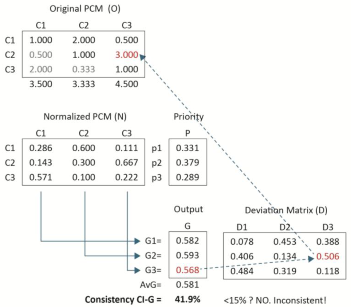
In this case, the cell (1,3) of the initial PCM (previous case, Figure 1) was changed from 6.000 to 0.500. To calculate the CI-G, a compatibility G analysis of the PCM’s columns with respect to its principal eigenvector or priority vector must be conducted, as shown in Figure 2.
The first and most important result, CI-G, is in bold and this time it shows an inconsistency value of 41.9%, much larger than 15% the ultimate lower limit (more confident if compared with 10% as the acceptable lower limit). This level significantly exceeds the maximum accepted threshold of 15%. So, the matrix is clearly inconsistent.
From Figure 2, it is evident that the smallest Gi (i.e., the least similar vector relative to the priority vector) in the Output column is G3, with a value of 0.568 (highlighted in red). This indicates that the third column is the source of the most important inconsistency, since G3 measures the degree of weighted similarity (compatibility) between the priority vector and the third column of the PCM in terms of weight and vector alignment.
To identify the specific component within the third column responsible for the greatest deviation, we identify the cell with the highest value. This cell represents the element contributing the largest weight and is, therefore, the most likely source of deviation (as indicated by the arrow in Figure 2). The subsequent blue arrow then points to the corresponding judgment in the original PCM, which should be carefully re-evaluated and, if necessary, revised.
By repeating this process iteratively, the PCM can be adjusted incrementally, improving its consistency. This iterative method is effective because it begins with the least compatible column, i.e., the one least aligned in terms of weight distribution and directional projection, and it refines the matrix toward an acceptable level of consistency.

3.3. Case 3: A 3 × 3 PCM with 3 Iterations of Consistency Adjustment

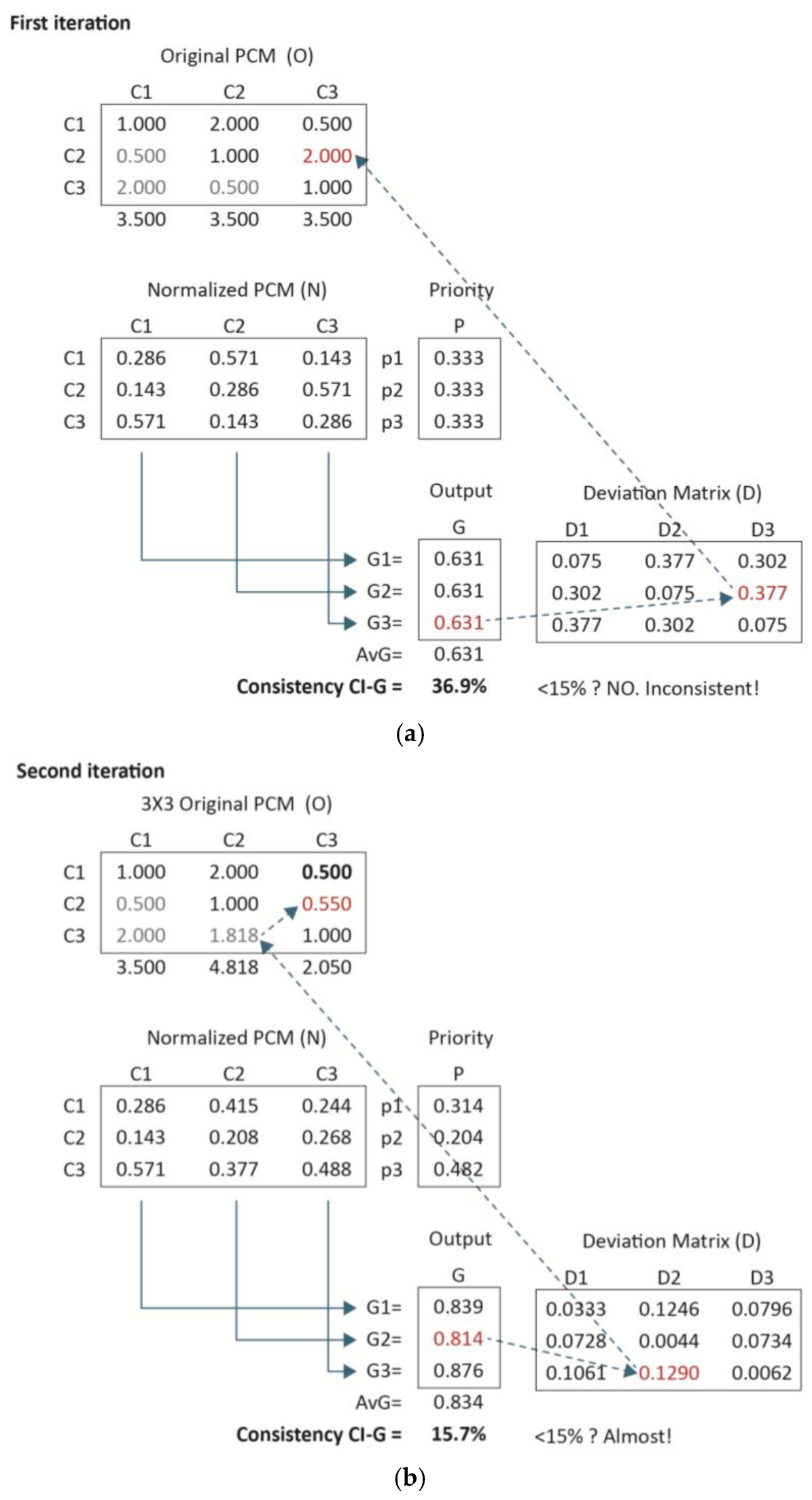
Next, an example of a 3 × 3 matrix evaluated across three iterations—aimed at achieving an acceptably consistent PCM—is presented in Figure 3a–c. The objective was to adjust the CI-G in order to reach a value below the accepted threshold, preferably under 15%, and ideally below 10%. This adjustment process required multiple iterations, as outlined below.
First iteration
This first iteration presents an interesting and noteworthy case, as all compatibility indices G are equal to 0.631. In this scenario, the strategy involves selecting the cell with the highest value in the deviation matrix. In this particular case, cell (2,3), which has a value of 0.377, is selected. It is worth noting that selecting cell (1,2)—which also has a value of 0.377—would yield the same process and outcome. Alternatively, choosing cell (3,1), with a value of 0.3772, would ultimately lead back to cell (2,3) in the original PCM, thereby producing the same adjustment result.
Second iteration
In the second iteration, the comparison judgment in PCM cell (2,3)—identified by the deviation matrix—was revised from 2.000 to 0.550. This adjustment effectively almost inverts the original value and was based on the presumption that a typographical error had occurred during the initial data entry into the PCM. The correction was implemented after consulting and reaching an agreement with the decision-maker regarding the suspected input error.
The second iteration reveals a matrix that is nearly consistent, with a CI-G value of 15.7%, which is marginally above the 15% threshold. The current sequence indicates that the inconsistency is now located in the second column. Specifically, G2 is the lowest compatibility index in the output set, with a value of 0.814. The highest deviation value within the second column is found in the third row (0.129), as indicated by the arrow.
Third iteration
Consequently, it is necessary to revise the original PCM value in cell (2,3). In this iteration, the value in PCM cell (2,3) is changed from 0.550 to 0.250. This adjustment also requires updating the reciprocal judgment in cell (3,2), as illustrated in Figure 3c.
Upon normalizing the matrix columns in the third iteration, all columns become identical to the priority vector, indicating that the convergence condition has been achieved. In this scenario, the matrix is fully consistent, with a CI-G value of 0%. This outcome is further validated by the deviation matrix, which is a null matrix, confirming the absence of deviations.
It may be noticed that transitivity improves with each iteration of the pairwise comparison matrix (PCM). This represents an interesting lateral effect of the CI-G procedure. Indeed, as compatibility increases, transitivity also tends to increase—though not necessarily at the same rate or pace. The CI-G consistency index links the initial and final priority vectors, thereby identifying the most effective path for enhancing consistency in the PCM (beyond transitivity) while taking the decision-making priorities into account.

3.4. Case 4: A 5 × 5 PCM with 3 Iterations of Consistency Adjustment

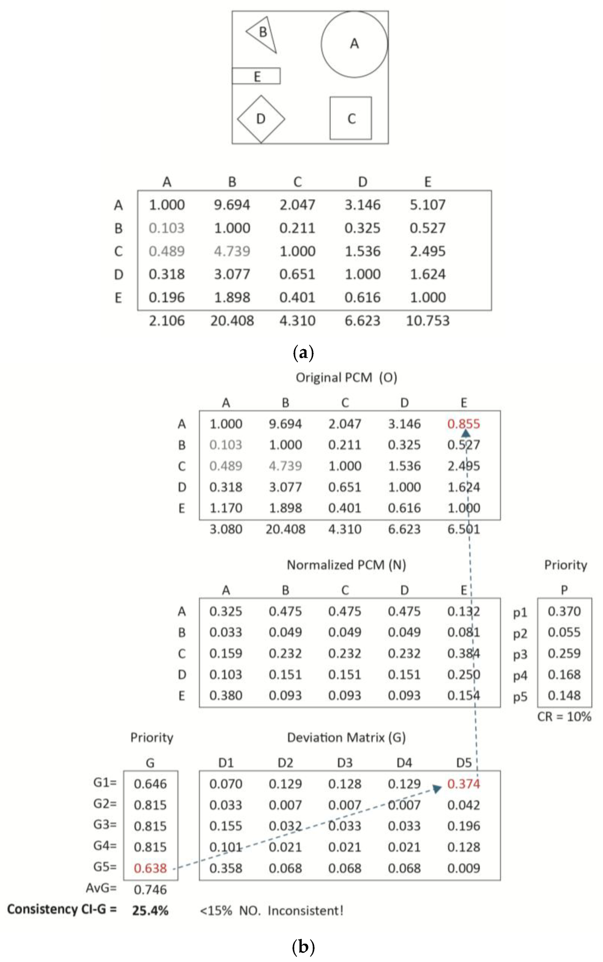
The following example features a 5 × 5 matrix, based on an “area validation example” as it is commonly referred to in the AHP/ANP literature [39]. In this scenario, five geometric figures are compared based on their respective areas, under the assumption that a larger area corresponds to greater priority as shown in Figure 4a. The approximate normalized area values for the geometric figures are as follows: Circle (A) = 0.475; Triangle (B) = 0.049; Square (C) = 0.232; Diamond (D) = 0.151; and Rectangle (E) = 0.093. Given that the pairwise comparisons reflect the actual relative areas of the figure, this PCM has perfect consistency; that is, CR = 0%.
Introducing an error in the circle-rectangle comparisons and analyzing consistency CR
Next, a small change will be introduced in this matrix as shown in Figure 4b. More specifically, all pairwise comparisons reflect the exact area ratios among the figures, with the exception of one: the comparison between Circle (A) and Rectangle (E). Here, an altered value of 0.855 is used, implying that Rectangle (E) is approximately 17% larger than Circle (A), which constitutes a significant comparison error, particularly because it involves the comparison of the largest element with the second smallest element in the set.
The CI-G is 25.4%, which substantially exceeds the minimum acceptable threshold of 15%. Consequently, it is necessary to revise the PCM in order to achieve an acceptable level of consistency. The smallest value in the Output G column is G5 = 0.638, and the largest deviation associated with this value in the deviation matrix occurs in cell (1,5). Accordingly, the next step is to examine the original PCM value corresponding to cell (1,5).
Some general observations can be made regarding this area-based example. CR calculated using the eigenvalue method yields a value of 10%, indicating acceptable consistency. However, cell (1,5) represents a comparison between the circle and the rectangle. A value of 0.855 implies that the rectangle is approximately 17% larger than the circle—despite the circle being more important and considerably larger. If these figures represented projects within an investment portfolio, such a comparison would lead to a significant misallocation of resources.
In general, the consistency index CR, based on the eigenvalue method, tends to be more lenient than the G index—sometimes excessively so. This occurs because the eigenvalue method does not account for the relative importance (weights) of the elements; it treats all comparisons as equally important. As shown previously (Equations (5)–(7)), CR = CI/RI is calculated as the deviation of the maximum eigenvalue from the matrix size (CI = λmax − n), divided by (n − 1), which corresponds to the average deviation of the eigenvalues excluding λmax. CI is divided by RI to adjust for the matrix size.
However, as with all arithmetic means, this average fails to consider the relative importance of the matrix elements. Dividing by (n − 1) implies that all deviations are equally significant, suggesting that an error involving the most important element is no more serious than one involving the least important. In this example, such averaging leads to a misleadingly acceptable CI of 10%. If we invert the comparison in cell (5,1), changing its value from 0.855 to 1.170, the CI-G still identifies the PCM as inconsistent (20.8% > 15%), while CR = 6% now indicates the matrix is highly consistent. A value of 2 (indicating the circle’s area is twice that of the rectangle’s) is required in the original PCM to reach the minimum acceptable consistency for CI-G (14.6% < 15%). To bring CI-G to around 10%, the input must reflect a value of 3 (indicating the circle is three times the size of the rectangle). The actual ratio between these two figures is approximately 5.
It is also worth noting that the compatibility index G between the true weight vector and the eigenvector derived from the altered PCM is 82.8%, slightly below the 85.0% threshold for acceptable compatibility. Statistically speaking, this suggests that the eigenvalue is not a grossly inaccurate approximation. However, if the goal is to ensure consistency aligned with the actual importance of the elements, that is, interpreting priority values as meaningful weights rather than just numerical entries, then, the CI-G index is the more appropriate consistency measure.
Introducing an error in the circle-triangle comparisons and analyzing consistency CR
To further illustrate the preceding point, the same area-based example was repeated, this time with a modified comparison between the circle and the triangle—the largest and smallest figures, respectively. In this scenario, not depicted as a figure, the circle was evaluated as only 1.5 times larger than the triangle, whereas in reality it is approximately 9.7 times larger. Despite this substantial error, the CR once again yielded an acceptable value of 10%. However, this discrepancy led to a 27.2% deviation in the largest figure, which would result in a significant misallocation of resources if the geometric areas were interpreted as project budget allocations. On the other hand, the CI-G yielded a 16.3% value, falling above the 15% accepted threshold for compatibility. This outcome reinforces the argument that in order to achieve a meaningful relationship between consistency and the actual weights, especially to avoid large deviations in high-priority elements, the CI-G provides a more reliable and informative measure of consistency than CR.
Another interesting feature observed in these examples is relative to the size of the matrix. It is well known that large matrices (>5) may produce inconsistency due to different factors such as the tediousness of the task for the decision maker and their lack of time. Using CI-G, the search for consistency errors is easy to accomplish and makes the pair comparison judgments easy to adjust. Still, the potential inconsistency challenges caused by matrix dimensions can be diluted by proper model structuring as discussed in Appendix C.
Consistency Ratio (CR) versus Consistency Index G (CI-G) behavior comparison
The following table illustrates how consistency indices CR and CI-G respond to variations in the comparisons between the circle and the rectangle, and the circle and the triangle, respectively. This comparison helps to assess the sensitivity and precision of each index.
Table 2 demonstrates that CR rapidly indicates consistency as the comparison ratios for a(1,5) (circle to rectangle) and a(1,2) (circle to triangle) approach their true values. In fact, CR suggests full consistency well before the actual ratios are reached, implying that inconsistencies may be “diluted” throughout the matrix. This dilution effect reduces the apparent impact of deviations in comparisons involving the most important (i.e., highly weighted) elements.
In contrast, the CI-G does not reach full consistency as quickly. CI-G continues to report high inconsistency until the comparison values closely align with the true ratios. Only when the input values nearly match the actual weights does CI-G indicate full consistency, thereby providing a more accurate and sensitive measure of deviation, particularly in comparisons involving the most influential elements.

3.5. Case 5: A 4 × 4 PCM with 3 Iterations of Consistency Adjustment

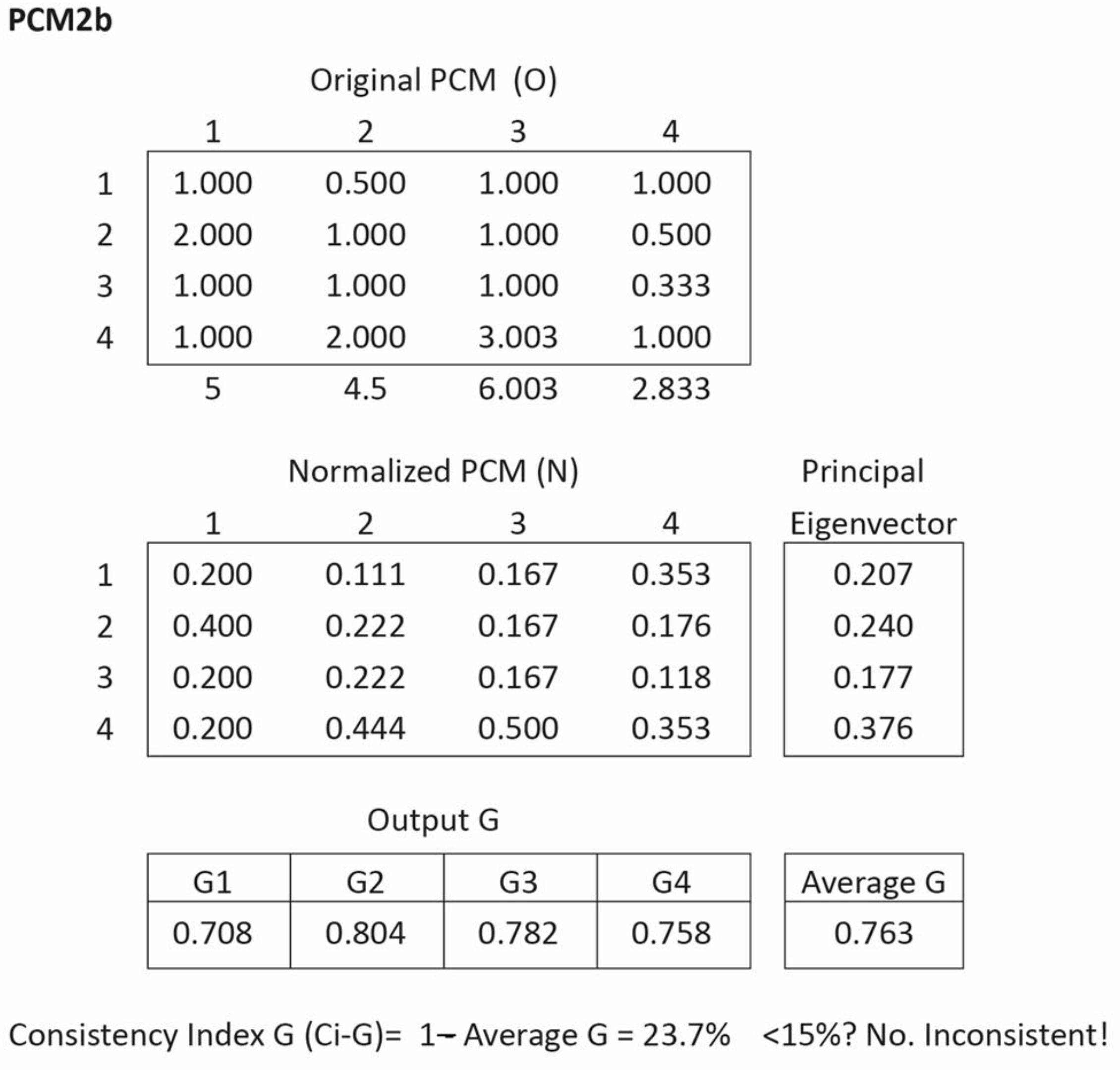
Next, Figure 5 illustrates an example of a 4 × 4 matrix, taken from [31], which shows a matrix that is 100% consistent, labeled PCM2a. Then, Figure 6 shows a perturbation in the PCM2b with the same principal eigenvector.
This is a matrix that is 100% consistent, as demonstrated by CI-G, CR, and Bose’s CI, as expected. Then, a perturbation is produced over the PCM, generating the next matrix, labeled PCM2b, with practically the same eigenvector (for all numerical purposes it is the same eigenvector).
The CI-G index indicates a highly inconsistent matrix, with a value of 23.7%, which exceeds the maximum acceptable threshold of 15%. In contrast, the CR and Bose’s consistency index both suggest that the matrix is consistent; the CR value is 9.0%, a borderline case for a 4 × 4 matrix according to CR’s inconsistency table. However, a critical question arises; how can a matrix be considered consistent when all of its column vectors are misaligned with the final eigenvector? As shown in Figure 6, none of the G values reach the minimum compatibility threshold of 0.85. It is also noteworthy that none of the four column vectors in the matrix approximate the two most significant entries in the eigenvector, i.e., cell 2 (0.2403) and cell 4 (0.3756), which correspond to the highest priorities in the priority vector. This misalignment is particularly problematic, as it occurs within the highest-weighted elements, precisely where inaccuracies have the most significant impact. Further elaboration on this issue is provided in Appendix A and Appendix B.
Remarkably, the same eigenvector can be derived from two vastly different PCMs—one fully consistent (regardless of the consistency index used), and the other highly inconsistent according to the CI-G, yet deemed consistent by both Saaty’s and Bose’s indices (albeit borderline in the former). This outcome is not surprising and is well-documented in graph theory; the eigenvector operator may converge on the same result (i.e., equilibrium point) from an infinite number of input configurations, not all of which are consistent or even close to consistency. This outcome also stems from the fourth property of the CI-G, namely, the lack of transitivity in compatibility. Specifically, it is possible for two individuals, A and B, to share the same priority vector C, with one exhibiting consistency and the other not.
To obtain an eigenvector associated with an acceptably consistent matrix, the CI-G guided improvement procedure can be applied. For instance, modifying the comparison in cell (1,2) from 0.50 to 1.0, and in cell (1,4) from 1.0 to 0.50, yields a new eigenvector (0.1948, 0.1948, 0.1768, 0.4336) with a CI-G value of 7.8%—below the 10% threshold. This revised matrix also shows near-perfect consistency under the consistency ratio index (CR = 0.1%). Although the new eigenvector differs from the original, the two remain compatible, with a compatibility index G of 90.0%—right at the threshold of acceptability.
This example demonstrates that two compatible (even identical) eigenvectors may originate from either consistent or inconsistent matrices. Therefore, eigenvector compatibility alone does not imply matrix consistency. Perturbations that leave the final eigenvector largely unchanged do not guarantee that the perturbed matrix is consistent. In fact, new comparison values may yield a PCM whose column vectors are entirely incompatible with the final eigenvector.
The above example highlights a fundamental insight. For a matrix to be acceptably consistent, the highest values in each column vector must align closely with the highest values in the final priority vector. It is important to note that CI-G is closely related to the compatibility index G; in fact, it represents the reverse side of the same coin. The G index is a metric that quantifies the proximity of two vectors based on both their weight and angular difference. This measurement approach has proven to be highly effective, thereby increasing confidence in the results produced by the CI-G consistency index. Given that the G index provides a robust metric for weighted spaces, the CI-G index inherits these desirable properties (see Appendix A).
This case also underscores a broader theoretical point—that the consistency threshold should be invariant with respect to the PCM. That is, it must be independent of the input data, matrix size, or even the eigenvector itself. This invariance ensures that different matrices can be assessed using a common consistency threshold, allowing for fair and meaningful comparisons. Ultimately, consistency should be measured by evaluating the closeness of vectors within their own weighted environments, as captured by the CI-G.
Table 3 presents a comparison of the most frequently cited consistency indices in the literature, based on a comprehensive review of AHP consistency indices from 1977 to 2021 [14]. In addition, other indices which are more recent or identified as relevant by the authors have been included in this table. The comparison is conducted using three key dimensions—weight, angle, and threshold—which, as previously discussed, are fundamental to any decision metric in a weighted environment (i.e., multicriteria decision making).
Table 3 demonstrates that the CI-G index is the only consistency measure that accounts for both weight and point-to-point projection explicitly; these two factors are essential when constructing the priority vector (i.e., the metric) in weighted environments. Moreover, it is the only index, with the inner dot product, that features a constant threshold value, independent of the PCM data or dimensionality.

4. Conclusions

This study introduces the CI-G as a novel and enhanced method for assessing the consistency of pairwise comparison matrices within the AHP/ANP. CI-G integrates weights, vector projection, and threshold analysis to identify the matrix element most suitable for targeted comparison improvement, thereby enhancing the reliability of decision outcomes.
A key conceptual contribution of this work is the interpretation of consistency as the compatibility of the PCM with itself, more specifically its principal eigenvector, offering a deeper perspective on consistency evaluation. Furthermore, the findings suggest that traditional consistency enforcement techniques may unintentionally impair the quality of the derived priority vector, underscoring the need for a judicious approach to consistency assessment.
A notable feature of CI-G is its definition of a consistency threshold as an absolute measure, independent of external parameters such as matrix size or input data. This property provides CI-G with robustness and broad applicability across diverse decision-making contexts.
Care must be taken to measure compatibility and consistency in a systematic manner. It is more important to align closely with the principal elements of the priority vector than with those of lesser importance. Not all indices are capable of accurately assessing compatibility or consistency in weighted environments.
Compatibility is more closely related to the intensity of preference rather than to the final ranking order. It is important to recognize that compatibility and rank order are not necessarily the same.

4.1. Limitations of the Study

Five case studies have been analyzed using the proposed CI-G, the relatively small number of consistency-focused applications represents a current limitation of this research. This constraint stems primarily from the innovative nature of the approach.
It is important to note, however, that the compatibility index G, on which CI-G is based, has already been widely applied in various fields—including artificial intelligence, pattern recognition, medical diagnostics, disaster risk management, environmental assessment, and resource allocation—with highly promising results. These outcomes provide a strong foundation for future research aimed at exploring the broader applicability of CI-G across decision-making frameworks and evaluating its influence on real-world AHP/ANP-based analyses.
In the context of the AHP, ordinal consistency (transitivity) is considered important for evaluating the rationality of PCMs. It serves as a criterion for determining the absence of self-contradiction in the decision maker’s preferences. Still, ordinal consistency may be considered as a necessary but insufficient condition to ensure consistency. Indeed, as stated by [50], the preferences may be logical and transitive, but the PCM can fail the consistency test. Furthermore, the opposite case is also possible and for this reason, techniques (e.g., linear optimization) have been proposed to assist decision-makers in satisfying both ordinal and cardinal consistency [50].
Given the above, ordinal consistency is not the focus of our analysis although the discussion of whether a satisfied CI-G meets the requirements of ordinal consistency is a valid research question to be explored in future studies. As previously explained, G is a cardinal value defined within the framework of order topology, making it a strong index that does not rely on ordinal relationships.

4.2. Future Research

Future research on the broader application of both the G and CI-G indices could explore their use along the Gini consensus index (GCI) or their potential as enhancements of the Jaccard distance measure, given that G constitutes a generalization of the Jaccard index for weighted environments [51].
Additionally, refining the threshold value by increasing the number of iterations in empirical testing could enhance the precision of the threshold, thereby improving both the accuracy and convergence behavior of the CI-G assessment.

Author Contributions

Conceptualization, C.G. and E.M.; Methodology, C.G. and E.M.; Formal analysis, C.G.; Investigation, E.M.; Writing—original draft, C.G.; Visualization, C.G.; Supervision, E.M. All authors have read and agreed to the published version of the manuscript.

Funding

This research received no external funding.

Data Availability Statement

The original contributions presented in this study are included in the article. Further inquiries can be directed to the corresponding author.

Conflicts of Interest

Author Claudio Garuti was employed by the Fulcrum Ingeniería Ltd. The remaining author declares that the research was conducted in the absence of any commercial or financial relationships that could be construed as a potential conflict of interest.

Abbreviations

The following abbreviations are used in this manuscript:
PCMPairwise comparison matrix
CI-GConsistency Index-G
AHPAnalytic hierarchy process
ANPAnalytic network process
CRConsistency ratio
RIRandom index

Appendix A. Compatibility and Consistency

Saaty’s idea of a correlation between compatibility and consistency that appears in his book “Principia Mathematica Discernendi” [23] (p. 128) is quite compelling and is the basis of our approach. However, the issue lies in the formula for computing compatibility, which, as previously mentioned, presents some problems. There are two main issues, described in descending order of severity [22].
First, let us review the procedure. A PCM is constructed from the resulting eigenvector (EV). This reconstruction invariably yields a matrix that is 100% consistent. The original PCM is then compared with this perfectly consistent matrix derived from the EV, using the Hadamard operator (element-wise matrix product) to compute the degree of compatibility as follows:
S = Hadamard(ABT) n−2 = (ΣiΣj aij (bij)−1) n−2
where the following apply:
S = Saaty’s compatibility index
A = the matrix produced by the eigenvector element ratios
BT = the original pair comparison reciprocal matrix transpose
n = matrix dimension
Problem 1:
Although this procedure may seem valid at first glance, the problem lies in the fact that the components of the eigenvector are arbitrary—they can be scaled in any way. Specifically, one can choose an eigenvector where the ratio between the largest and smallest components is arbitrarily large. This leads to a serious issue when applying the A1 equation for compatibility, as it produces a singularity (divergence) that results in arbitrarily large incompatibility values. If vector incompatibility is interpreted as the lack of projection of one vector (or matrix in Hadamard case) onto another, then such extreme values make no sense. Vectors cannot be more incompatible (or compatible) than 100% (i.e., it is not possible to be more perpendicular than 100% orthogonal with zero projection, or more parallel than 100% with full projection). Thus, values beyond the 0–1 range are conceptually meaningless. This singularity or divergence can also be demonstrated mathematically [22,51,52].
Problem 2:
A second issue in equation A1 arises from the division by n square (n2), which essentially averages the row and column means. However, this “average of averages” disregards (twice) the relative importance of the involved variables (i.e., it assumes all elements are equally weighted, which is unrealistic). While this technical issue might be addressed, for example by using a weighted average, as done in [52], the more fundamental problem described above will persist.
A final idea to present is that the compatibility (and consistency by extension) is a priority vector matter or an EV matter when using this systemic operator to obtain the priority vector. This is because the space of measurement in weighted environments is well defined by the eigenvector and not by the PCM where it came from, since it is the eigenvector that has all the comparison combined in order to have the actual preferences in the equilibrium point. Thus, it is the eigenvector that contains the actual information that must be used for measurement in weighted environments. The PCM is the precursor to the eigenvector not the metric of measurement itself, just like a blueprint is the precursor to the building not the building itself. Considering this, then compatibility and consistency must be calculated using the eigenvector data (where the metric of the PCM take place).
Compatibility Index Analysis: G Index vs. Others Approaches
There are several other compatibility indices in the extant literature. Table A1 lists some popular ones.
Table A1. Different compatibility indices in the literature.
Saaty’s compatibility index:C(A,B) = [ΣiΣj aij (bij)−1] n−2
Garuti’s compatibility index (G index):C(A,B) = ½ Σ((ai + bi)Min(ai,bi)/Max(ai,bi))
Hilbert’s compatibility index:C(A,B) = Log(Max(ai/bi)/Min(ai/bi)
Inner vector product inverted:C(A,B) = (Σaibi−1)/n
Weighted inner vector product inverted:C(A,B) = Σa(i)b(i)−1w(i))
Euclidean formula normalized: C(A,B) = SQRT(½Σ(ai − bi)2)
Source: [22].
A case-based sensitivity analysis for each of the previously listed compatibility indices is presented in Table A2.
Table A2. Comparison of different compatibility indices.
Vector
Coordinates
Hadamard Prod.(1-G)Hilbert’s1-IVP1-Euclidean
Saaty’s IndexGaruti’s IndexIndexDot Prod. Normal.
CaseParallel TrendDistance or Incompatibility
00.5000.5001.010%9.523%8.715%1.010%5.000%
0.4500.550
10.5330.4670.058%2.371%2.097%0.218%1.200%
0.5450.455
20.6330.3670.068%2.369%2.259%0.760%1.200%
0.6450.355
30.7330.2670.097%2.363%2.702%1.548%1.200%
0.7450.255
40.8330.1670.198%2.348%3.860%3.161%1.200%
0.8450.155
50.9330.0671.108%2.285%9.126%10.274%1.200%
0.9450.055
60.9870.013280.851%1.839%111.919%599.399%1.200%
0.9990.001
70.999000.001002452.727%0.149%200.043%4949.950%0.099%
0.999990.00001
CasePerpendicular TrendDistance or Incompatibility
00.5000.5000.28%9.523%8.72%5.56%5.00%
0.5500.450
10.5330.4672.76%14.471%13.58%64.40%7.80%
0.4550.545
20.6330.36736.32%43.504%49.61%17.61%27.80%
0.3550.645
30.7330.267153.63%64.680%90.42%61.65%47.80%
0.2550.745
40.8330.167630.74%80.808%143.45%178.56%67.80%
0.1550.845
50.9330.0675931.69%93.780%242.26%751.73%88.30%
0.0500.950
60.9870.0131,896,128.85%99.291%487.99%49,250.65%98.60%
0.0010.999
70.99990.0001249,994,999.976%99.999%999.999%4999.5%99.998%
0.00010.9999
Source: [22].
The conclusion from Table A2 is that the only compatibility index that consistently performs well across all cases is the G index. It maintains outcomes within the 0–100% range (similar to the normalized Euclidean formula), which is a critical condition, as values outside this range are difficult to interpret and may indicate potential divergence. It is also noteworthy that the G index results in Table A2 are closely aligned with those of the normalized Euclidean formula, yet they demonstrate greater accuracy and sensitivity to variation. This is because G is not based on absolute differences as distance metrics are, but rather on relative absolute ratio scales, as employed in AHP/ANP.
In contrast, the Euclidean distance formula reveals no variation in the distance of parallel trends from Case 1 to Case 6. In other words, the Euclidean-based index fails to capture differences in compatibility because the absolute differences between coordinates remain constant. Consequently, one might incorrectly conclude, based on the Euclidean-based index, that there is no variation in vector compatibility across Cases 1 to 6. This leads to the erroneous inference that Case 1 is as incompatible as Cases 2 through 6, which contradicts the expected outcome. This counterintuitive behavior arises from the fact that the Euclidean formula relies solely on absolute differences and does not account for the relative importance of the coordinates.
It is important to recognize that the values within the priority vector represent intensities of preference. In the context of proximity or similarity, it is more meaningful to be closer to a higher-preference value (i.e., a larger coordinate) than to a lower one. Additional tests conducted in higher-dimensional spaces (ranging from 3D to 10D) confirm this trend. Moreover, as the dimensionality of the space increases, the likelihood of divergence among compatibility indices also rises, except in the cases of the G and Euclidean indices, as demonstrated by Cases 6 and 7 in Table A2 for both parallel and perpendicular trends.
It is also noteworthy that the G function depends on two distinct dimensional factors: (1) the intensity of preference, associated with weight information and reflecting an order topology concept, and (2) the angular projection between vectors. This implies that G is a function of both preference intensity and the angular relationship between vectors, expressed as G = f(I, α). This formulation indicates that G is not merely a dot product (though it may appear so), but rather a more nuanced and complex function. Both preference intensity and angular distance are implicitly embedded within the coordinates of the priority vector and must be accurately extracted to construct a meaningful compatibility index. The same reasoning applies to consistency indices, as consistency and compatibility represent two sides of the same coin.
The Importance of a Cardinal Compatibility Index
We emphasize here the importance of having a cardinal rather than an ordinal compatibility index. In this regard, one can find diverse kind of consistency indices based on ordinal preferences, some relative to transitivity in the PCM, and others relative to the preservation of (ordinal) order preference (POP) of the decision-maker (DM). It is straightforward to demonstrate that the G index is not strictly dependent on the ordinal preferences of the DM, even though this may be assumed at first glance. Consider the following scenario. Two candidates, A and B, are running for election, and three individuals (P1, P2, and P3) must decide between them. P1 prefers A (A > B), while P2 and P3 prefer B (B > A). P1 and P2 are moderate, expressing preference intensities of 55% for A and 45% for B, and 45% for A and 55% for B, respectively. P3, however, is an extremist, with a 5% preference for A and 95% for B.
Is P2 really more compatible (more aligned) with P3 simply because they made the same choice? This example demonstrates that sharing the same ordinal preference is insufficient to define compatibility. This is a crucial insight, and aligns with the broader conclusion that Arrow’s Impossibility Theorem applies to ordinal preferences and can potentially be bypassed when working within a cardinal preference framework. A numerical example follows (Table A3).
Table A3. Numerical Example: Cardinal vs. Ordinal Preferences.
Decision-MakerCardinal PreferencesOrdinal Preferences
P1{0.364; 0.325; 0.311}1 2 3
P2{0.310; 0.325; 0.365}3 2 1
P3{0.501; 0.325; 0.174}1 2 3
Table A3 shows that no unique ordering is possible under ordinal preferences alone. However, using cardinal values and the G compatibility index, a meaningful ordering can be established, as follows:
  • G(P1, P2) = 0.90 (90%) → Compatible
  • G(P1, P3) = 0.77 (77%) → Not compatible
  • G(P2, P3) = 0.70 (70%) → Not compatible
Despite sharing the same ordinal preferences, P1 and P3 are not compatible. Conversely, although P1 and P2 have opposite ordinal rankings, they are compatible. This can be interpreted as evidence that individuals who vote for the same candidate do not necessarily share the same value system or reasoning process. True compatibility only becomes apparent when preference intensities are considered.
This conclusion reinforces the idea that value systems are better reflected by cardinal measures of preference rather than ordinal rankings. It also explains why the G compatibility index is rooted in order topology theory rather than metric topology. Furthermore, this insight is equally relevant for consistency analysis, since improving ordinal transitivity within the PCM does not necessarily reflect the real underlying value system embedded in the priority vectors—only the (weighted) cardinal structure does.
In summary, ordinal measure should not be used in compatibility or consistency measure.
Performance Comparison of the G Index with Others Compatibility Indices
Another comparison of the performance between the G index and other compatibility indices is worth recalling. Consider the following example involving the relative electricity consumption of household appliances [41].
Table A4. Relative electric consumption household appliances.
AlternativesABCDEFGW
(Eigenvector)
Actual
Electric range (A)12587990.3930.392
Refrigerator (B)1/21455790.02610.242
TV
(C)
1/51/4125680.1310.167
Dishwasher (D)1/81/51/214990.1100.120
Iron
(E)
1/71/51/51/41590.0610.047
Hair-dryer (F)1/91/71/61/91/5150.0280.028
Radio
(G)
1/91/91/81/91/91/510.0160.003
Source: [39].
Although the eigenvector (W) and the actual values may initially appear to be close, a deeper assessment is warranted. When evaluated using different compatibility indices—namely, Saaty’s compatibility index (S), the Hilbert compatibility index (H), the inverse vector product (IVP), and the G index—the following results are obtained:
S = 1.455 → 45.5% > 10% → Incompatible vectors
H = 1.832 → 83.2% > 10% → Incompatible vectors
IVP = 1.630 → 63.0% > 10% → Incompatible vectors
G = 0.920 → 92.0% > 90% → Compatible vectors
These results indicate that the W and actual vectors are incompatible according to the S, H, and IVP indices, but they are compatible according to the G index, as anticipated.
An intriguing observation emerges when the weight of the “radio” alternative decreases to a certain threshold: the compatibility indices—Saaty’s (S), Hilbert’s (H), and the inverse vector product (IVP)—may exceed 100%, signaling extreme incompatibility. This raises an important geometric question: can two vectors be “more perpendicular” than 100%? Geometrically, this notion is counterintuitive, as orthogonality is maximized at 90°. However, values exceeding 100% suggest that the vectors diverge in a manner that surpasses conventional perpendicularity under these metrics. Such results may indicate a form of directional opposition or structural misalignment that these indices amplify beyond standard geometric interpretation.
Next, we examine a few examples drawn from [53] which presents several instances that highlight the unnecessary and at times hazardous use of fuzzy set theory within the analytic hierarchy process (AHP) when constructing metrics for decision-making.
The objective of this exercise is to evaluate the quality of the constructed metrics by assessing their compatibility with actual values. Specifically, we aim to determine how closely the fuzzy set-based metrics align with actual values in comparison to those derived through conventional AHP. This leads us to pose the following questions: Which approach yields more accurate results? Does the use of fuzzy sets provide any advantage? Or conversely, does it result in greater deviation from actual values compared to traditional AHP outcomes?
Three examples are selected from [44], “Fuzzy Judgment and Fuzzy Sets”. The G index is applied to evaluate the quality (i.e., a quality test) of the metrics obtained from both conventional AHP and fuzzy AHP, by comparing them with the actual values.
Example A1.
Estimation of GNP for Different Countries.
Table A5. Estimation of GNP for different Countries.
AlternativesMetric by AHPActual GNP Values (1972) Metric by Fuzzy AHP
US0.4270.4130.469
USSR0.2300.2250.184
China0.0210.430.030
France0.0520.0690.063
UK0.0520.0550.060
Japan0.1230.1040.107
W.Germany0.0940.0910.087
Compatibility of the MetricG = 92.6% > 90%
→ Compatible
G = 88.2% < 90%
→ Incompatible
Source: [22].
As Table A5 shows, the metric obtained using the eigenvector method is closer to the actual metric than the one derived from fuzzy sets (92.6% vs. 88.2% of compatibility). Therefore, the use of fuzzy sets does not enhance metric quality; in fact, it slightly degrades it.
Example A2.
Estimation of Weight for Different Objects.
As can be seen in Table A6, there is non-relevant value added to the metric quality using fuzzy sets (94.2% vs. 95% of compatibility).
Table A6. Estimation of weight for different objects.
AlternativesMetric by AHPActual WeightsMetric by Fuzzy AHP
Radio0.090.100.081
Typewriter0.400.390.406
Large Attache Case0.200.200.193
Projector0.290.270.28
Small Attache Case0.040.040.04
Compatibility of the MetricG = 94.2% > 90%
→ Compatible
G = 95% > 90%
→ Compatible
Source: [53].
Example A3.
Estimation of most expensive car.
Table A7 demonstrates that the use of fuzzy sets does not add value to the metric quality—in fact, it slightly worsens it.
** Additionally, for the alternative 3 (Acura-TL), the fuzzy set metric produces a ranking error, placing it third instead of fifth. However, the overall compatibility of the fuzzy set metric remains within an acceptable range (though it constitutes a borderline case).
Table A7. Estimation of most expensive car.
AlternativesAHP MetricActual CostFuzzy AHP Metric
Mercedes0.23710.24530.247
BMW0.23030.22640.231
Acura-TL0.15160.14150.190 **
Lexus-ES0.18740.18870.063
Audi-AG0.19350.19810.168
Incompatibility of the MetricG = 97.2% > 90%
→ Compatible
G = 89.9% (Borderline case)
Source: [53].

Appendix B. Equation (1) Numerical Demonstration

The following demonstration is explained in detail in [22] and also discussed in [20,54], but a brief summary is provided here for the convenience of the reader.
Preposition A1.
Index G is a positive real number between 0 and 1.
Suppose we have two vectors A and B with coordinates as follows:
A: {0.1; 0.9} and B= {0.9; 0.1}. Hint: these are two very different vectors almost perpendicular vectors in the geometrical representation.
The value of G is:
G = 0.5 × (0.1 + 0.9) × (Min(0.1;0.9)/Max(0.1;0.9) + Min(0.9;0.1)/Max(0.9;0.1))
G = 0.5 × 1 × (0.1/0.9 + 0.1/0.9) = 0.1111 (11.1%). This is a compatibility value in the 0–1 interval and geometrically represents almost perpendicular vectors.
It is also interesting to note that the incompatibility (1 − G) of these two vectors is: 1 − 0.1111= 0.8888 (88.9%) which is close to the (traditional) distance calculation value in metric topology (D = 0.8) for this set of coordinates.

Appendix C. When the Inconsistency Source Is Not Located in the PCM

Consistency in the AHP/ANP models is an index related in general to one matrix at the time. However, a weighted average of consistency index CI-G for the entire hierarchy can be expressed as follows:
CI-GH = {Σh Σi(Wi,hCI-Gi,h+1)}H1 i = 1…n° of criteria in level h; h = hierarchy level
where the following apply:
CI-GH = Consistency index G of the entire hierarchy (as a weighted average).
Wi,h = Global weight of criterion “i” at level h.
CI-Gi,h+1 = Consistency index CI-G of the matrix under criterion “i” at level (h + 1).
H = Number of levels of the hierarchy.
If CI-GH is less or equal than 0.1 (10%), then, the consistency of the entire hierarchy is acceptable.
This calculation of the CI-G for the entire hierarchy it may serve as an indicator of potential issues within the AHP model. Regarding such modeling issues, it is very important to clarify that AHP and/or ANP structures may influence the assessment of the consistency index. Indeed, the modeling process is often not well taken care of, especially with regard to the homogeneity issue.
There are two groups of cases of homogeneity issues, as follows:
Case A1.
One element is much smaller than the others (more than one order of magnitude).C << A, B.
Suppose we have a 3 × 3 matrix with the triad: A = 3B; B = 4C and A = 9C. In this case, the 3 × 3 matrix has a CI-G = 5.3% < 10% (a very good consistency). But what if the triad is A = 4B; B = 7C and A = 9C ? Now, the consistency is CI-G =18.4%, far from the 10% of threshold; thus, it is not an acceptable consistency. (Even if we try an extreme comparison value of A = 9.9C, then the CI-G = 16.9%, which is still larger than the acceptable threshold).
In the first triad, we would need A = 12C, and in the second, A = 24C to be fully consistent. But Saaty’s scale only goes from 1 to 9; this limitation is clearly exposed in Axiom 2 of the AHP (the homogeneity axiom). This axiom is needed because the human mind has trouble comparing elements that are farther apart than one order of magnitude (for instance, comparing the size of an elephant with an ant). This kind of comparison may produce a lack of consistency in the PCM; a small lack of consistency if the elements to be compared are close to one order of magnitude or a lack of consistency strong if the difference is big, as shown in the results of the two previous examples.
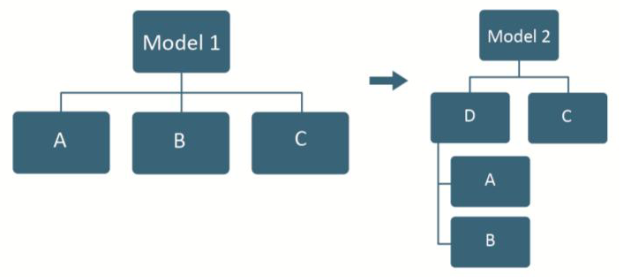
In those cases, the adjustment of consistency is not in the PCM but in the AHP/ANP model itself. It is necessary to modify the AHP model, from model 1 to model 2, creating a new element D “father” of C, commensurable with A and B (same order of magnitude) and one or more element E (or even more elements), siblings of C, as shown in the next figure.
Note: C plus E, gives the necessary relative importance to D in order to be commensurable with A and B.
Figure A1. One element is much smaller than the others: Moved to a lower level.
Mathematics 13 02666 g0a1
Notice that some AHP criticisms are due to this basic modeling error.
This outcome suggests that the model is missing an entire branch. For example, the D branch might require greater depth (i.e., additional hierarchical levels) and more criteria at each level. This situation indicates that the initial model is flawed—incomplete rather than incorrect—and that criterion C serves as a signal or warning that a critical component may be absent from the model.
Alternatively, a second solution—often the simpler and sometimes the correct one—would be to remove criterion C. This is appropriate when the C element is clearly irrelevant to the decision problem at hand.
This solution is presented in the next figure:
Figure A2. One element is much smaller than the others: Deleted from the hierarchy.
Mathematics 13 02666 g0a2
In terms of the number of comparisons, Case A1 demonstrates a gain in the second example, as some criteria were removed. Conversely, the first example entails a loss in terms of added comparisons, since additional criteria—potentially an entire branch—must be added. However, this increase in comparisons is justified by a far more significant outcome: the development of a higher-quality model.
Case A2.
One element is much larger than the others (more than one order of magnitude). C >> A, B.
Since node C is much larger than nodes A and B, we need to add a new criterion (Node D) above nodes A and B (clustering nodes A and B) and with (approximately) the same importance of node C, that is, within (or close to) one order of magnitude among nodes D and C.
Figure A3. One element is much larger than the others: A new element is added.
Mathematics 13 02666 g0a3
Notice that passing from Model 1 to Model 2, we have not just improved the consistency index in the initial model (Matrix A,B,C), but we also have fewer pair comparisons to make (three in model 1 vs. two in model 2). This is true for any matrix size in model 1. For instance, going from a 4 × 4 matrix in model 1 (with six comparisons) to three matrices of 2 × 2 (three comparisons in total), or one matrix of 3 × 3 plus one matrix of 2 × 2 in model 2 (4 comparisons in total). It is notable that the bigger matrix size in model 1 (breaking the homogeneity axiom) provides a bigger gain with fewer comparisons in model 2 (without breaking the homogeneity axiom).

References

  1. Ishizaka, A.; Mu, E. What is so special about the Analytic Hierarchy and Network Process? Ann. Oper. Res. 2023, 326, 625–634. [Google Scholar] [CrossRef]
  2. Saaty, T.L. What is the analytic hierarchy process? In Mathematical Models for Decision Support; Springer: Boston, MA, USA, 1988; pp. 109–121. [Google Scholar]
  3. Brunelli, M. Introduction to the Analytic Hierarchy Process; Springer: New York, NY, USA, 2015. [Google Scholar]
  4. Saaty, T.L. Scaling Method for priorities in hierarchical structures. J. Math. Psychol. 1977, 15, 234–281. [Google Scholar] [CrossRef]
  5. Crawford, G.B. The geometric mean procedure for estimating the scale of a judgment matrix. Mathl. Model. 1987, 9, 327–334. [Google Scholar] [CrossRef]
  6. Aguaron, J.; Moreno-Jimenez, J. The geometric consistency index: Approximated threshold. Eur. J. Oper. Res. 2003, 147, 137–145. [Google Scholar] [CrossRef]
  7. Fedrizzi, M.; Civolani, N.; Critch, A. Inconsistency evaluation in pairwise comparison using norm-based distances. Decis. Econ. Financ. 2020, 43, 657–672. [Google Scholar] [CrossRef]
  8. Lamata, M.T.; Peláez, J.I. A method for improving the consistency of judgments. Int. J. Uncertain. Fuzziness 2002, 10, 677–686. [Google Scholar] [CrossRef]
  9. Pelaéz, J.; Lamata, M. A new measure of consistency for positive reciprocal matrices. Comput. Math. Appl. 2003, 46, 1839–1845. [Google Scholar] [CrossRef]
  10. Benitez, J.; Delgado-Galván, X.; Gutierrez, J.A.; Izquierdo, J. Balancing Consistency and Expert Judgment In AHP. Math. Comput. 2011, 54, 1785–1790. [Google Scholar] [CrossRef]
  11. Benitez, J.; Delgado-Galván, X.; Izquierdo, J.; Pérez-García, R. Achieving Matrix Consistency in AHP Through Linearization. Appl. Math. Model. 2011, 35, 4449–4457. [Google Scholar] [CrossRef]
  12. Koczkodaj, W.W. A new definition of consistency of pairwise comparisons. Math. Comput. Model. 1993, 18, 79–84. [Google Scholar] [CrossRef]
  13. Duszak, Z.; Koczkodaj, W.W. Generalization of a new definition of consistency for pairwise comparisons. Inf. Process. Lett. 1994, 52, 273–276. [Google Scholar] [CrossRef]
  14. Pant, S.; Kumar, A.; Ram, M.; Klochkov, Y.; Sharma, H.K. Consistency Indices in Analytic Hierarchy Process: A Review. Mathematics 2022, 10, 1206. [Google Scholar] [CrossRef]
  15. Saaty, T.L. Theory and Applications of the Analytic Network Process; RWS Publications: Pittsburgh, PA, USA, 2005. [Google Scholar]
  16. Saaty, T.L. Decision Making with Dependence and Feedback: The Analytic Network Process; RWS Publications: Pittsburgh, PA, USA, 1996. [Google Scholar]
  17. Saaty, T.L.; Peniwati, K. Group Decision Making: Drawing out and Reconciling Differences; RWS Publications: Pittsburgh, PA, USA, 2008. [Google Scholar]
  18. Salomon, V.; Shimizu, T. Performance of three different methods of multiple criteria decision making applied to the supplier selection. In Proceedings of the 18th International Conference of MCDM Chania, Chania, Greece, 19–23 June 2006. [Google Scholar]
  19. Mu, E. A unified framework for site selection and business forecasting using ANP. J. Syst. Sci. Syst. Eng. 2006, 15, 178–188. [Google Scholar] [CrossRef]
  20. Garuti, C. Measuring compatibility (closeness) in weighted environments. In Proceedings of the International Symposium of the Analytic Hierarchy Process, Viña del Mar, Chile, 6 August 2007. [Google Scholar]
  21. Garuti, C.; Salomon, V. Compatibility indices between priority vectors. Int. J. Anal. Hierarchy Process 2012, 4, 152–160. [Google Scholar] [CrossRef]
  22. Garuti, C. Measuring in Weighted Environments: Moving from Metric to Order Topology; Universidad Tecnica Federico Santa Maria Press: Santiago de Chile, Chile, 2012. [Google Scholar]
  23. Saaty, T.L. Principia Mathematica Decernendi: Mathematical Principles of Decision Making; RWS Publications: Pittsburgh, PA, USA, 2010. [Google Scholar]
  24. Pereyra-Rojas, M.; Mu, E.; Gaskin, J. The Higher-Ed Organizational-Scholar Tension: How Scholarship Compatibility and the Alignment of Organizational and Faculty Skills, Values and Support Affect Scholar’s Performance and Well-Being. Front. Psychol. 2017, 8, 450. [Google Scholar] [CrossRef]
  25. Leon, Y.L.; Mu, E. Organizational MIndfulness Assessment and Its Impact on Rational Decision Making. Mathematics 2021, 9, 1851. [Google Scholar] [CrossRef]
  26. Garuti, C. A set theory justification of Garuti’s compatibility index. J. Multicriteria Decis. Anal. 2019, 27, 50–60. [Google Scholar] [CrossRef]
  27. Ovchinnikov, S. Functional Analysis: An Introductory Course; Springer: Cham, Switzerland, 2018. [Google Scholar]
  28. Brunelli, M.; Fedrizzi, M. Axiomatic properties of inconsistency indices for pairwise comparisons. J. Oper. Res. Soc. 2015, 66, 1–15. [Google Scholar] [CrossRef]
  29. Saaty, T.L. Decision Making for Leaders: The Analytic Hierarchy Process; McGraw-Hill: New York, NY, USA, 1980. [Google Scholar]
  30. Miller, G. The magical number seven, plus or minus two: Some limits on our capacity for processing information. Psychol. Rev. 1956, 63, 81–97. [Google Scholar] [CrossRef]
  31. Bose, A. Consistency re-evaluation in analytic hierarchy process based on simulated consistent matrices. J. Multicriteria Decis. Anal. 2022, 29, 393–401. [Google Scholar] [CrossRef]
  32. Garuti, C.; Mu, E. A Rate of Change and Center of Gravity Approach to Calculating Composite Indicator Thresholds: Moving from an Empirical to a Theoretical Perspective. Mathematics 2024, 12, 2019. [Google Scholar] [CrossRef]
  33. Ishizaka, A.; Labib, A. Review of the main developments in the analytic hierarchy process. Expert Syst. Appl. 2011, 38, 14336–14345. [Google Scholar] [CrossRef]
  34. Pelaéz, J.; Martinez, E.A.; Vargas, L.G. Consistency in Positive Reciprocal Matrices: An Improvement in Measurement Methods. IEEE Access 2018, 6, 25600–25609. [Google Scholar] [CrossRef]
  35. Salomon, V.A.P.; Gomes, L.F.A.M. Consistency Improvement in the Analytic Hierarchy Process. Mathematics 2024, 12, 828. [Google Scholar] [CrossRef]
  36. Sato, Y.; Tan, K.H. Inconsistency indices in pairwise comparisons: An improvement of the Consistency Index. Ann. Oper. Res. 2023, 326, 809–830. [Google Scholar] [CrossRef]
  37. Srdjevic, B.; Srdjevic, Z. Prioritisation in the analytic hierarchy process for real and generated comparison matrices. Expert Syst. Appl. 2023, 225, 120015. [Google Scholar] [CrossRef]
  38. Garuti, C. Reflections on scales from measurements, not measurement from scales. Int. J. Anal. Hierarchy Process 2017, 9, 349–360. [Google Scholar] [CrossRef]
  39. Garuti, C. New advances of the compatibility index “G” in weighted environments. Int. J. Anal. Hierarchy Process 2016, 8, 514–536. [Google Scholar] [CrossRef]
  40. Wu, Z.; Tu, J. Managing transitivity and consistency of preferences in AHP group decision making based on minimum modifications. Inf. Fusion 2021, 67, 125–135. [Google Scholar] [CrossRef]
  41. Whitetaker, R.W. Validation examples of the Analytic Hierarchy Process. Math. Comput. Model. 2007, 46, 840–859. [Google Scholar] [CrossRef]
  42. Barzilai, J.; Cook, W.D.; Golany, B. Consistent weights for judgments matrices of the relative importance of alternatives. Oper. Reearch Lett. 1987, 6, 131–134. [Google Scholar] [CrossRef]
  43. Kendall, M.G.; Smith, B.B. On the method of paired comparisons. Biometrika 1940, 31, 324–345. [Google Scholar] [CrossRef]
  44. Barzilai, J. Consistency measures for pairwise comparison matrices. J. Multi-Criteria Decis. Anal. 1998, 7, 123–132. [Google Scholar] [CrossRef]
  45. Stein, W.E.; Mizzi, P.J. The harmonic consistency index for the analytic hierarchy process. Eur. J. Oper. Res. 2007, 177, 488–497. [Google Scholar] [CrossRef]
  46. Golden, B.L.; Wasil, A.E.; Harker, P.T. An Alternative Measure of Consistency. In The Analytic Hierarchy Process: Applications and Studies; Golden, B.L., Wasil, A.E., Harker, P.T., Eds.; Springer: Berlin/Heidelberg, Germany, 1989; pp. 68–81. [Google Scholar]
  47. Ramik, J.; Koviny, P. Inconsistency of pair-wise comparison matrix with fuzzy elements based on geometric mean. Fuzzy Sets Syst. 2010, 161, 1604–1613. [Google Scholar] [CrossRef]
  48. Salo, A.; Hamalein, R. On the measurement of preference in the analytic hierarchy process. J. Multi-Criteria Decis. Anal. 1997, 6, 309–319. [Google Scholar] [CrossRef]
  49. Wu, Z.; Xu, J. A consistency and consensus based decision support model for group decision making with multiplicative preference relations. Decis. Support Syst. 2012, 52, 757–767. [Google Scholar] [CrossRef]
  50. Kou, G.; Lin, C. A cosine maximization method for the priority vector derivation in AHP. Eur. J. Oper. Res. 2014, 235, 225–232. [Google Scholar] [CrossRef]
  51. Mazurek, J.; Ramik, J. Some new properties of inconsistent pairwise comparisons matrices. Int. J. Approx. Reason. 2019, 113, 119–132. [Google Scholar] [CrossRef]
  52. Del Moral, M.J.; Trillo, J.R.; Perez, I.J.; Tapia-Garcia, C.; Tapia, J.M. An Alternative Consensus Measure Based on the Gini Index for Group Decision-Making Problems. J. Adv. Comput. Intell. Intell. Inform. 2025, 29, 379–388. [Google Scholar] [CrossRef]
  53. Soon, M. Notes on the Use of Compatibility Index in the Analytic Hierarchy Process. In Proceedings of the International Symposium of the Analytic Hierarchy Process 2020, Virtual, 3–6 December 2020. [Google Scholar]
  54. Saaty, T.L. Fuzzy Judgments and Fuzzy Sets. Int. J. Strateg. Decis. Sci. 2008, 1, 18. [Google Scholar] [CrossRef]
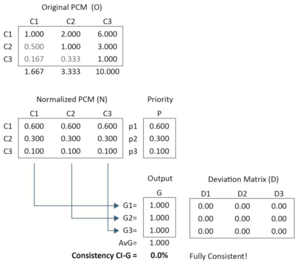
Figure 1. 3 × 3 fully consistent PCM.
Mathematics 13 02666 g001
Figure 2. Inconsistent 3 × 3 PCM with its priority vector and CI-G.
Mathematics 13 02666 g002
Figure 3. (a) 3 × 3 PCM, first iteration. (b) 3 × 3 PCM, second iteration. (c) 3 × 3 PCM, third iteration.
Mathematics 13 02666 g003aMathematics 13 02666 g003b
Figure 4. (a) Figure shapes and their relative’s exact areas in a 5 × 5 PCM. (b) 5 × 5 PCM and the associated consistency adjustments.
Mathematics 13 02666 g004
Figure 5. 4 × 4 100% Consistent PCM. Source: [31].
Mathematics 13 02666 g005
Figure 6. 4 × 4 PCM with small perturbation. Source: [31].
Mathematics 13 02666 g006
Table 2. PCM Consistency Index G (CI-G) range and its relation to it priority vector compatibility.
Precision Test (Circle to Rectangle)Precision Test (Circle to Triangle)
a(1,5)CRCI-Ga(1,2)CRCI-G
0.8510%21.6%1.5410%23.3%
1.256%20.8%27%20.8%
22%14.6%42%13.1%
31%8.7%51%10.2%
40%4.2%6.500%6.4%
5.100%0.0%9.700%0.0%
Exact Ratio, Circle to Rectangle = 5.11Exact Ratio, Circle to Triangle = 9.69
Source: Authors.
Table 3. Comparison of CI-G with Different Consistency Indices.
ItemConsistencyWeightProjectionThreshold
(Index)(Importance)(Alignment)(Independent?)
0CI-GSatisfiesSatisfiesYes
1 CI [4]DissatisfiesDissatisfiesNo
2 CI+ [13,40]DissatisfiesDissatisfiesNo
3GCI [41] DissatisfiesDissatisfiesNo
4CM [12,13] DissatisfiesDissatisfiesNo
5RE [42] DissatisfiesDissatisfiesNo
6HCI [43]DissatisfiesDissatisfiesNo
7GW [44] DissatisfiesDissatisfiesNo
8NIσn [45]DissatisfiesDissatisfiesNo
9CMSH [46] DissatisfiesDissatisfiesNo
10CIH [47]DissatisfiesDissatisfiesNo
11CCI [48]Partially SatisfiesSatisfiesNo
12RIC [49]Partially SatisfiesDissatisfiesNo
13Bose CR [31]DissatisfiesDissatisfiesNo
14Inner dot product inverted [22]DissatisfiesSatisfiesNo
Source: Adapted from [14]. Note: Any consistency index must meet the three proposed conditions of weight, projection and threshold independence to be considered equivalent to the proposed CI-G.
Disclaimer/Publisher’s Note: The statements, opinions and data contained in all publications are solely those of the individual author(s) and contributor(s) and not of MDPI and/or the editor(s). MDPI and/or the editor(s) disclaim responsibility for any injury to people or property resulting from any ideas, methods, instructions or products referred to in the content.