Article

Combined Optimization of Both Sensitivity Matrix and Residual Error for Improving EIT Imaging Quality

1
School of Mathematics, Yili Normal University, Yili 835001, China
2
School of Electrical and Information Engineering, Tianjin University, Tianjin 300072, China
*
Author to whom correspondence should be addressed.
Mathematics 2025, 13(16), 2663; https://doi.org/10.3390/math13162663
Submission received: 10 July 2025 / Revised: 5 August 2025 / Accepted: 15 August 2025 / Published: 19 August 2025

Abstract

As a visual detection technique, Electrical Impedance Tomography (EIT) can reconstruct the distribution of electrical parameters within a detection field. EIT reconstruction greatly depends on a physical equation that includes a sensitivity matrix and measurements, but the sensitivity matrix fails to be optimized for various reconstruction tasks. This issue decreases the applicable range of the physical equation and EIT reconstruction quality. To address this issue, this paper optimizes both the residual error for measurements and the sensitivity matrix in the equation, which leads to higher EIT reconstruction quality. The optimization solution is theoretically and experimentally verified. Results indicate that the proposed methods can reduce the relative error of EIT reconstruction quality by about 12.0%.

1. Introduction

Electrical Impedance Tomography (EIT) is widely applied in industrial inspections and medical diagnostics due to its rapid, non-invasive, low-cost, and non-radioactive characteristics [1,2]. However, the imaging quality of EIT is constrained by its inherent ill-posedness and soft-field effects [3,4]. Consequently, the development of high-quality EIT imaging algorithms has become an area of interest.
The quality of EIT imaging depends on the selected algorithm and the available measurements. Existing EIT algorithms include direct and indirect examples [5]. The direct imaging algorithms include the most widely used examples, such as linear back projection [6], algebraic reconstruction [7], D-bar [8], and so on. Nonparametric algorithms usually rely on optimization techniques and related algorithms, such as conjugate gradient [9], Tikhonov regularization [10], and adaptive reweighting [11], etc. To date, although almost all indirect algorithms have a fast response, their imaging quality is often too low to satisfy actual requirements. Optimization algorithm-based imaging algorithms have gradually become the primary focus in practice. According to various actual requirements, these indirect algorithms focus on the following three aspects:
(1) Improving the distance measure: Guo et al. [12] combined the Alternating Direction Method of Multipliers (ADMM) with the Ant Lion Optimizer (ALO), and an enhancement in imaging resolution was achieved. Wang et al. [13] utilized the residual term L2 norm and the regularization term (resistivity L1 norm) as the loss function, achieving fast and high-quality image reconstruction with the Split Bregman iterative algorithm. Wang et al. [14] employed the deep prior embedding method for generalizing the residual term and improving the EIT reconstruction quality.
(2) Improving the regularization matrix: Shi et al. [15] integrated first-order and second-order TV regularization terms and further refined the image reconstruction process by adjusting the weights between these TV terms. Xu et al. [16] introduced a novel neighborhood-based regularization method, employing the total difference between neighboring pixels as the regularization term, thereby effectively enhancing spatial resolution.
(3) Improving the sensitivity matrix: Liu et al. [17] used an efficient multitask structure-aware sparse Bayesian learning for frequency difference EIT, where the sensitivity matrix was reformulated. Yang et al. [18] derived four different types of higher-order approximate sensitivity matrices, including the traditional sensitivity matrix, using integral equations to mitigate the soft-field effect. Liu et al. [19] began from the perspective of compressed sensing, represented the distribution of electrical parameters using a Fourier basis, and reconstructed the sensitivity matrix.
In this paper, two nonlinear optimization algorithms are developed to improve EIT imaging accuracy and reliability. Different from existing methods, the new algorithms can simultaneously optimize both the residual error and the sensitivity matrix. Moreover, the theoretical and practical foundations of the optimization process are verified to ensure their generalizability.

2. Related Work

The EIT techniques mainly include Electrical Resistance Tomography (ERT) [20], Electrical Capacitance Tomography (ECT) [21], and Electrical Magnetic Tomography (EMT) [22], all of which have similar mathematical expressions. Thus, we only emphasize ERT. This section first introduces the ERT principles that are in accordance with the Maxwell equation. Then, the related algorithms utilized to validate the method of this study are introduced.

ERT Principle

Let Ω represent a circular ERT detection field bounded by ∂Ω, to which m measurement electrodes are attached, as shown in Figure 1a.
We use a typical 16-electrode ERT system to illustrate the ERT principle [23]. The detection field, Ω, has a boundary, ∂Ω, on which 240 measurements are available for reconstructing a frame of an ERT image. Let Ω be partitioned into n units (pixels), and let σ be the normalized conductivity vector of n units, σ = (σ1, σ2, …, σn)T. The ERT aims to determine the conductivity distributions of n units based on 240 measurements on ∂Ω: u1, u2, …, u240, denoting U = (u1, u2, …, u240)T. Based on the finite element method [24], the linearized and discrete natural relationship from σ to U can nearly be expressed as
U = , s.t., UΩ, σ ∈ Ω
where S is called the sensitivity distribution matrix in the EIT imaging process, which provides a linear map of the units (pixels) from σ to U. To solve σ along with U, S is usually determined in advance.
To solve the variable σ in Equation (1), the LBP has the highest time resolution among all the EIT algorithms owing to no need for any iterations, but it has very limited imaging quality. Usually, the inverse matrix S−1 is taken as the transport matrix of S to solve σ.
σ = S−1U, s.t., S−1 = ST
Due to the easy realization and the widest application, we regard the LBP as the benchmark algorithm and compare it with our proposed novel algorithm in this paper.
On the other hand, our previous study [25] demonstrated that any measurement, ui, consists of the positive effect of all the pixels in Ωi+ and the negative effect of those in Ωi (see Figure 1b), where Ωi+ and Ωi refer to the two sets of units in Ω in which all pixels have positive and negative sensitivity coefficients for the ith measurement, respectively. It is necessary to distinguish between the two kinds of opposite effects. Any measurement ui can be decomposed into two new measurements, ui+ and ui, which are computed by
u i + = u i / ( 1 + S i / S i + ) u i = u i / ( 1 + S i + / S i ) ,   i = 1 , 2 , , n
where Si+ and Si are the sum of all positive sensitivity coefficients and all negative sensitive coefficients in the sensitivity matrix S for ui, respectively. Hence, ui+ is larger than ui and can raise the ERT quality, whereas ui is opposite.
In this paper, the measurement decomposition method is used to improve the resolution of each measurement and simultaneously reduce the soft-field effect, just as it was successfully applied in our previous research.

3. Various Objective Functions for Improving the EIT Reconstruction Quality

This section has two parts: one outlines our motivation of constructing various sensitivity matrixes, and the other provides the solutions of the objective function and its performances.

3.1. Sensitivity Matrix Analysis

The following analysis of the sensitivity matrix S starts with an analysis of the sum of the sensitivity coefficients. The measurement data used in the existing EIT process is obtained from the difference between boundary measurements after the excitation and measurement of the empty field and the full field, respectively; the empty field is an assumed homogeneous field, while the full field is the object field corresponding to the actual target. The EIT process usually solves the sensitivity coefficients in S from the null field and assumes that the null field (reference field) and the full field (detection field) obey the same sensitivity coefficients—an assumption that introduces a significant error into image reconstruction [26]. Figure 2 shows the calculated sensitivity coefficients in S in the COMSOL6.1 simulation environment, where 1–2 are used as the excitation electrodes and 6–7 are used as the measurement electrodes.
Figure 2a shows the schematic of the simulation model. Figure 2b,c show the distribution of the sensitivity coefficients in S for the empty field and the full field, respectively, from which it can be seen that there is a great difference between the sensitivity coefficients of the empty and the full field. Figure 2 shows that there is a significant increase in the sensitivity coefficient of the target region compared to the empty field. In fact, there is a highly nonlinear relationship between the sensitivity coefficients of the empty field and the full field. Therefore, the calculation of the sensitivity coefficient is extremely critical to the EIT reconstruction process.
To further illustrate the role of the sensitivity coefficients, we observe that for the pixels corresponding to the target region in the sensitivity matrix S, the sum of the sensitivity coefficients corresponding to all excitation and measurement modes are different in the null and full fields on the EIT reconstruction, as shown in Figure 3a,b.
Taking the EIT with 812 pixels for 16 electrodes as an example, we assume that the subscripts j1, j2, …, jT in the null field correspond to the target region of T pixels. Then, we multiply a factor m to each column of the sensitivity coefficients relative to T pixels, where m is greater than zero. This multiplication makes the effect of the T pixels in the target region is greater than their original value in S. But when m is less than 1, this means that it the effect of the T pixels in the target region is less their original value. In this way, we replace all the pixels in the target region to obtain a new full-field sensitivity coefficients matrix, S′, as shown in Figure 3b. This process is equivalent to multiplying the coefficients m to the T columns of S corresponding to the target region.
Figure 4a shows the simulation model of the Chinese character “津”, which refers to a target field, and Figure 4b shows the distribution of the sum of the sensitivity coefficients in S after multiplying by a factor of 0.1 all columns relative to the target field, denoting it as S′. It can be seen that the sum of the sensitivity coefficients in S′ approximately target object distributions. Using the same measurements and the TR algorithm based on S and S′, the reconstructed images are shown in Figure 4c,d. The model is recognized after using S’, while the target object distribution is not recognized using S.
Therefore, the target object distributions in the EIT reconstruction can be represented by the sum of sensitivity coefficients in S′. In fact, almost all EIT iterative algorithms represent an attempt to optimize the sum of the spatial columns relative to the target objects such that their respective sums are more convergent to the actual individual pixel electrical parameter values. However, the existing EIT algorithms apply global optimization, and their ability to obtain the local information of each column is greatly limited. Therefore, with the aim of directly optimizing the sensitivity coefficients of each column in S, the following two novel optimization algorithms are proposed after providing sufficient theoretical basis. First, according to the basic principle of EIT reconstruction, the original constraints in the existing method are retained, and the nonlinear objective function is reconstructed. Hence, a Nonlinear Programming-based Difference Minimization (NLP-DM) is proposed. Then, in an effort to exchange the objective function with the constraints, a Nonlinear Programming-based Target-Constraint Swap (NLP-TCS) is proposed, as explained below.

3.2. NLP-DM Optimization and Solution

For the typical EIT algorithm, the constraints of the NLP-DM algorithm remain a set of linear constraints. Its objective function contains residual errors with squared terms and remains a nonlinear optimization problem. By minimizing the difference between the grey vector, g, and the sum of the elements in each column in the sensitivity matrix, S, it is possible to better describe the key information in EIT reconstruction.
The NLP-DM algorithm is defined as
min F ( S , g ) = j = 1 n ( i = 1 m s i j g j ) 2 ,             s . t . ,     S g = U ,     g 0
where sij is the element in the sensitivity matrix, S = {sij}, and g = (g1, g2, …, gn)T. U = (u1, u2, …, um)T, m is the number of measurements, and n is the number of pixels.
Noting that H = [ 1 ,   ,   1 ] 1 × m T , the transformation of Equation (4) is
min F ( S , g ) = < S T H g , S T H g > ,   s . t . , S g = U , g 0
where <,·> is the inner product.
λ = (λ1, λ2, …, λn)T such that the Lagrange function of Equation (5) is
L ( g , λ ) = < S T H g , S T H g > λ T ( S g U )
then, it satisfies
F / λ = S g U F / g = 2 ( g S T H ) S T λ
The equation of the stationary point is
S g U = 0 g = S T ( H + λ / 2 )
It leads to
S S T ( H + λ / 2 ) = U
Notice that SgU = 0. There must be a solution, so the sign “+” is the generalized inverse of the matrix. It follows from
( S S T ) ( S S T ) + U = U
This shows that SST (H + λ/2) = U. Thus, the general solution is
H + λ / 2 = ( S S T ) + U + ( I ( S S T ) ( S S T ) + ) y
where y is an arbitrary number. Thus,
g = S T ( S S T ) + U + S T ( I ( S S T ) ( S S T ) + ) y
Notice that
S T ( S S T ) ( S S T ) + = S T
Therefore, the solution of the NLP-DM for EIT is
g = S T ( S S T ) + U
where (SST)+ is the generalized inverse matrix. Hence, adding an adjusting parameter λ and IRm×m, the diagonal matrix I is introduced to avoid the appearance of singular square matrices, which translates directly into the solution of the inverse matrix. Therefore, the optimized solution can be further reformulated as
g = S T ( S S T + λ I ) 1 U
As a result, after adjusting the value of λ, the EIT inverse problem can be solved, and all objects in the detection field can be reconstructed.
The NLP-DM algorithm must converge. In fact, From F(St, gt) at the tth iteration to F(St+1, gt+1), the objective function of NLP-DM again undergoes two iterations:
(1)
Solving the vector St+1 from F(St, gt) to F(St+1, gt) after fixing gt;
(2)
Solving the vector gt+1 from F(St+1, gt) to F(St+1, gt+1) after fixing St+1.
The optimizations on (1) and (2) ensure convergence according to the Lagrange optimization condition. Hence, the following inequalities hold:
F(St, gt) ≤ F(St+1, gt) ≤ F(St+1, gt+1)
Thus, {F(St, gt)} is a decreasing sequence and is bounded. According to the theorem on “Monotonic bounded sequences must converge” [27], the NLP-DM must converge.

3.3. NLP-TCS Optimization and Solution

The construction of the NLP-TCS algorithm is based on an in-depth analysis of the NLP-DM algorithm, in which the objective function of the NLP-DM determines the constraints of the NLP-TCS, while the constraints of the NLP-DM are transformed into the objective function of the NLP-TCS algorithm. This algorithm achieves the swapping of the objective function and the constraints with a view to optimizing the EIT reconstruction process from different perspectives.
Further, additional coefficient variables are introduced into the NLP-TCS to improve its adaptability to uncertainties in the imaging process by adjusting to influence the quality of the image reconstruction.
Thus, the objective of the NLP-TCS algorithm is to minimize the sum of the squares of the differences between the measured values and the weighted decision values while satisfying a set of linear constraints between the weighted sensitivity elements and the grey scale. Therefore, the NLP-TCS algorithm for the EIT reconstruction is defined as
min F ( C , g ) = i = 1 m ( j = 1 n c j s i j g j u i ) 2 ,             s . t . ,   i = 1 m c j s i j = g j   , g j 0
where cj is the jth coefficient in C; C = (c1, c2, …, cn)T; and cj and gj are all unknowns, where j = 1, 2, …, n.
Equation (16) is, in fact, an unconstrained optimization problem, since
c j = g j / i = 1 m s i j
Then, the optimization problem can be transformed into
min F ( C , g ) = i = 1 m ( j = 1 n s i j g j 2 / k = 1 m s k j u i ) 2
Let h j = g j 2 , t i j = s i j / k = 1 m s k j ; then, the problem is transformed to
min h j 0 i = 1 m ( j = 1 n t i j h j u i ) 2
i.e.,
min h j 0 T h U , T h U = min h j 0 T h U 2
Then, T is actually the normalized sensitivity matrix, and it is turned into
min h j 0 T h U 2
The solution to Equation (21) can iteratively be obtained using the iterative Newton-Raphson gradient descent or conjugate gradient descent [27].

3.4. Simulation Results

In order to verify the effectiveness of the proposed optimization algorithms, NLP-DM and NLP-TCS, in solving the EIT problem, they are employed in simulation experiments comparing them with the typical LBP algorithm.
The simulation includes six models, as shown in the first row of Table 1, where red denotes the target objects and blue denotes the background ones, and their conductivities are set to 1 and 2 S/cm, respectively. The experiments were carried out in the EIT single-electrode excitation-measurement mode, and the detection field is partitioned into 812 grids (pixels) such that m = 240 and n = 812. A PC implements the simulations with an Intel® Core™ i5-12400F 2.50 GHz processor with 16 GB RAM, COMSOL6.1, and MATLAB2020.
All the EIT images are evaluated by (1) comparing the original and reconstructed images and (2) evaluating the spatial resolution via two indexes: Correlation Coefficient (CC) and Relative Error (RE). The CC between the reconstructed and the reference (actual) images is defined as
C C = i = 1 n ( σ i σ 0 ) ( σ i * σ 0 * ) { i = 1 l ( σ i σ 0 ) 2 i = 1 l ( σ i * σ 0 * ) 2 } 1 / 2
where CC denotes the correlation coefficient; σ is the calculated conductivity; σ* is the actual conductivity in the simulated or experiment distribution; σi and σi* are the ith elements of σ and σ*, respectively; σ0 and σ0* are the mean values of σ and σ*, respectively; and n denotes the number of pixels in Ω. The RE is defined as
R E = | σ σ * | / | σ * |
The two indexes noted above have been widely used to evaluate the imaging quality in most ERT reconstruction processes and relative methods [11,12,13,14,15,16,17,18].
The LBP, NLP-DM, and NLP-TCS algorithms are used to reconstruct all target objects in the six models based on the same measurements, respectively. These measurements are normalized to weaken the influence of soft-field effects. Afterwards, the NLP-DM is solved by using Equation (20) with appropriate parameter values. The Landweber algorithm [28] is used for pre-iteration before using the NLP-DM. The first-order pre-iterative null field sensitivity matrix S is used to improve the accuracy and the convergence. The comparison of the sum of the sensitivity coefficients in S before and after the pre-iteration is shown in Figure 5, which clearly shows that the middle part of the EIT detection field is more sensitive, thus bringing the reconstructed image closer to the real model.
For the NLP-TCS, we use Equation (21) as the objective function to reconstruct the EIT image based on the sensitivity matrix, S, before pre-iteration. In order to improve the computational efficiency of the NLP-TCS, the conjugate gradient descent method is used to solve the optimal solution, and the number of iterations is set to ITER = 20. Over the six models, the reconstruction results of the three algorithms are shown in Table 1.
The best reconstructed images result from NLP-TCS for all four models, except for the best reconstructed images of Models II and VI, in which the best images result from the NLP-DM. In these images, the positions of all targets can be correctly reconstructed. The NLP-DM reconstructs the target size more accurately and reconstructs the image with a clear background. In particular, the imaging artifacts of NLP-TCS are generally smaller, and the boundaries of the targets are more clearly defined, which may be attributed to the optimized process by the NLP-TCS during the iterative process. In contrast, all images from LBP contain artifacts, and partial target objects are incorrectly connected together or are covered by artifacts. Consequently, the imaging quality of NLP-DM or NLP-TCS is better than that of the existing LBP algorithm, and most detected objects can be found in these reconstructed images.
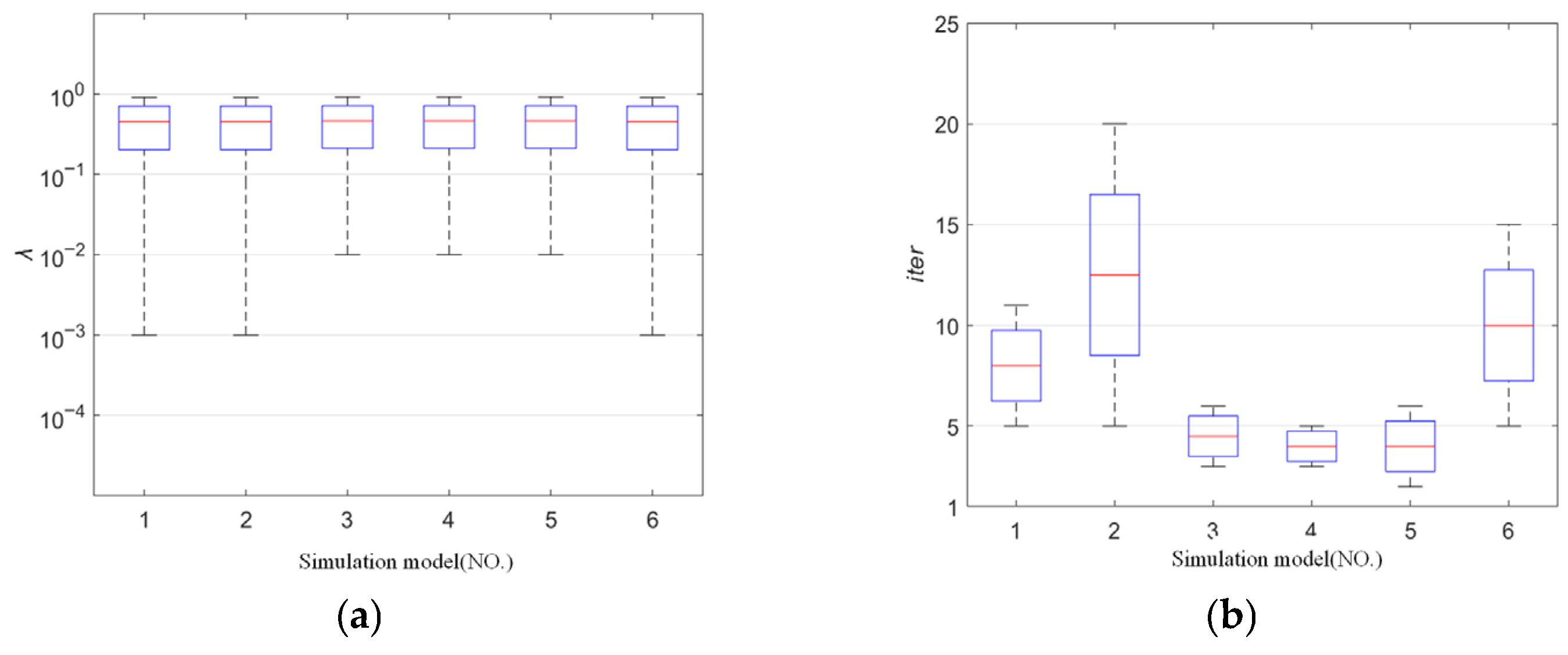
Since the hyperparameter λ has an impact on the reconstruction quality of the NLP-DM, and the number of iterations (ITER) of the NLP-TCS also affects the computation time and reconstruction accuracy of the NLP-TCS. We also traverse the discrete λ value sets to evaluate the effectiveness of the NLP-DM and NLP-TCS algorithms for image reconstruction for these six models. Among them, λ is set to [10−5, 1], which is discretized into 50 subintervals, and the number of iterations (Iter) is set to [1, 50], which is discretized into 50 sub-intervals. Based on the RE values, the λ values and the number of iterations (Iter) for the better imaging of each model are determined for both the NLP-DM and NLP-TCS algorithms. The optimal distribution of values is shown in Figure 6.
It can be seen that all the models in the NLP-DM have optimal λ values taken in the interval [10−3, 100], and the medians are located near 10−1, indicating that the optimal values can be taken in most cases where λ = 10−1. The optimal iteration numbers of all models in the NLP-TCS algorithm are all below 15, indicating that in most cases, fewer iterations can reconstruct a better image; the minimum value is no more than 5, indicating that the NLP-TCS algorithm can converge quickly, and in most cases, the optimal number of iterations is 5. At the same time, the interquartile ranges of most of the models were narrow, with most of the λ values and Iter values being concentrated in smaller ranges, and the range between the minimum and maximum values is also smaller. Therefore, it can be concluded that the hyperparameters in the NLP-DM algorithm (λ) and the number of iterations in the NLP-TCS algorithm (Iter) are generalized and robust, and taking values within a certain range does not affect the optimization stability of the NLP-DM and NLP-TCS algorithms.
The evaluation metrics RE, CC, and runtime are further utilized to quantitatively represent the above imaging observations (see Table 2). As shown in the metrics data in the table, the RE values of the NLP-DM and NLP-TCS algorithms are lower than those of the LBP algorithm for all six models, indicating that these two optimization algorithms are able to reconstruct images more accurately. The two proposed methods can reduce the relative error of EIT reconstruction quality by about 12.0%. Meanwhile, the CC values of the NLP-DM and NLP-TCS algorithms are generally higher than those of the LBP algorithm, which indicates that these two optimization algorithms are able to better capture the features of the target object in the image and thus achieve higher imaging relevance.

3.5. Real Experiments

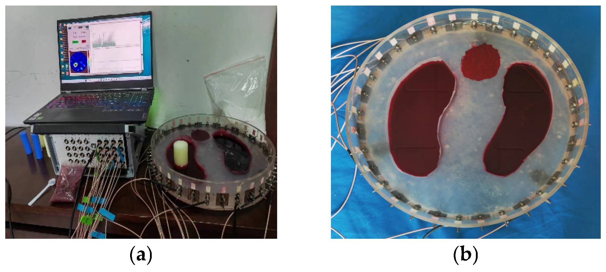
In order to further verify the effectiveness of the two nonlinear optimization algorithms in practical applications, we conducted a series of experimental tests and analyzed the experimental results. The experiment used the EIT system designed and manufactured by the laboratory, as shown in Figure 7a, for testing.
The experimental model simulates lung tissue and the thoracic environment using agar powder and saline solution. The simulated lungs and hearts are wrapped in saline solution with a conductivity of 1.55 µS/cm. Rubber sticks simulate tumors in lung tissue, with the detection target being simulated lung tumors. The empty field (reference field) is set to simulate tumor-free lung tissue and the heart, as shown in Figure 7b. The full field (detection field) refers to the detection field with tumors, and the first row in Table 3 represents the four models to be detected.
In the actual experiments, the algorithm parameter settings were consistent with those in the simulations. Based on the same measurement data, all target objects in the four models were reconstructed using LBP, NLP-DM, and NLP-TCS algorithms, and the reconstruction results are shown in Table 3.
It can clearly be seen that the two nonlinear optimization algorithms, NLP-DM and NLP-TCS, have clear target recognition, fewer artifacts, and better imaging quality than the traditional LBP algorithm. Moreover, the imaging results of both algorithms, especially the NLP-TCS algorithm, are significantly higher than those of the LBP algorithm. It can be seen that the three algorithms have good recognition performance for a tumor model (Model 1 and Model 2), but the NLP-DM and NLP-TCS algorithms are less affected by the position and quantity of the target object compared to the LBP algorithm. At the same time, it can be seen that although it is a heterogeneous background, the imaging quality is not significantly affected by the background because the measurement values corresponding to the background are used as the empty field data. Compared to the LBP algorithm, which has artifacts in the imaging background, and some targets are incorrectly connected together (see Model 3), the NLP-DM and NLP-TCS algorithms have clearer targets and are less affected by background media. The observation results once again confirm that the two optimization algorithms have good robustness.
We further utilize evaluation indicators RE and CC to quantify the observation results of the above imaging process, as shown in Table 4. From the indicator data in the table, it can be seen that in the presence of noise in the measured values in the actual environment, the NLP-DM and NLP-TCS algorithms have smaller RE and larger CC on all four models, resulting in better imaging quality. In particular, the NLP-TCS algorithm has higher imaging accuracy, more accurate detection of target positions, and higher correlation.

4. Conclusions

Dual optimization methods based on sensitivity coefficients and residual errors are proposed to overcome the limitations of existing EIT reconstruction algorithms in handling complex imaging. By introducing nonlinear programming methods, the imaging quality and stability have been enhanced. The nonlinear optimization algorithms, NLP-DM and NLP-TCS, are both derived from a solid theoretical basis and therefore have strong generalization ability. The new objective function and constraints in the two algorithms are instructive and can guide the optimization of sensitivity coefficients in the imaging process. In simulation and practical experiments, the effectiveness of the two algorithms is verified based on typical evaluation indicators such as relative error and the correlation coefficient. The proposed dual optimization method has the potential to further deepen EIT image reconstruction, providing new theoretical and practical support for improving the quality of EIT image reconstruction.
With the advancement of deep learning technology and more effective mathematical analysis, there are currently a number of research directions with promising application prospects, such as the deep prior embedding method for electrical impedance tomography [14], tensor-based representation [29], and the sparse Bayesian method [30]. These directions are instructive, and we will focus on them in the future.

Author Contributions

Conceptualization, J.G. and Q.X.; Data curation, Q.X.; Resources, J.G.; Software, J.G.; Supervision, S.Y.; Writing, S.Y. and Q.X. All authors have read and agreed to the published version of the manuscript.

Funding

(1) The Yili Normal University Special Project for Enhancing the Comprehensive Strength of Disci-plines (Key) (No.: 22XKZZ17); (2) The Yili Normal University High level Cultivation Project (Key) (No.: YSPY2022012).

Data Availability Statement

All data is available in the attachment of this submission.

Conflicts of Interest

The authors declare no conflicts of interest.

References

  1. Zhang, Q.; Mo, H.; Li, R.; Liang, C.; Luo, J.; Bespal’Ko, A.A. Image reconstruction method based on wavelet fusion in electrical capacitance tomography with rotatable electrode sensor. Measurement 2024, 238, 115354. [Google Scholar] [CrossRef]
  2. Dong, F.; Yue, S.; Liu, X.; Wang, H. Determination of hyperparameter and similarity norm for electrical tomography algorithm using clustering validity index. Measurement 2023, 216, 112976. [Google Scholar] [CrossRef]
  3. Wang, Z.; Liu, X. A regularization structure based on novel iterative penalty term for electrical impedance tomography. Measurement 2023, 209, 112472. [Google Scholar] [CrossRef]
  4. Cui, Z.; Wang, H.; Xu, Y.; Zhang, L.; Yan, Y. An integrated ECT/ERT dual modality sensor. In Proceedings of the 2009 IEEE Instrumentation and Measurement Technology Conference, Singapore, 5–7 May 2009; pp. 1434–1438. [Google Scholar] [CrossRef]
  5. Sun, J.; Yang, W. A dual-modality electrical tomography sensor for measurement of gas–oil–water stratified flows. Measurement 2015, 66, 150–160. [Google Scholar] [CrossRef]
  6. Zhang, K.; Li, M.; Yang, F.; Xu, S.; Abubakar, A. Three-dimensional electrical impedance tomography with multiplicative regularization. IEEE Trans. Biomed. Eng. 2019, 66, 2470–2480. [Google Scholar] [CrossRef]
  7. Clay, M.T.; Ferree, T.C. Weighted regularization in electrical impedance tomography with applications to acute cerebral stroke. IEEE Trans. Med. Imaging 2002, 21, 629–637. [Google Scholar] [CrossRef]
  8. Hamilton, S.J.; Hauptmann, A. Deep D-bar: Real-time electrical impedance tomography imaging with deep neural networks. IEEE Trans. Med. Imaging 2018, 37, 2367–2377. [Google Scholar] [CrossRef]
  9. Dyakowski, T.L.; Jeanmeure, F.; Jaworski, A.J. Applications of electrical tomography for gas–solids and liquid–solids flows—A review. Powder Technol. 2000, 112, 174–192. [Google Scholar] [CrossRef]
  10. Murphy, E.K.; Mahara, A.; Halter, R.J. A novel regularization technique for microendoscopic electrical impedance tomography. IEEE Trans. Med. Imaging 2016, 35, 1593–1603. [Google Scholar] [CrossRef]
  11. Nie, F.; Wang, X.; Huang, H. Multiclass capped p-norm SVM for robust classifications. In Proceedings of the AAAI, San Francisco, CA, USA, 4–9 February 2017; pp. 2415–2421. [Google Scholar] [CrossRef]
  12. Guo, H.; Liu, S.; Guo, H. Hybrid iterative reconstruction method for imaging problems in ECT. IEEE Trans. Instrum. Meas. 2020, 69, 8238–8249. [Google Scholar] [CrossRef]
  13. Wang, J.; Ma, J.; Han, B.; Li, Q. Split Bregman iterative algorithm for sparse reconstruction of electrical impedance tomography. Signal Process. 2012, 92, 2952–2961. [Google Scholar] [CrossRef]
  14. Wang, J.W.; Deng, J.S.; Liu, D. Deep prior embedding method for Electrical Impedance Tomography. Neural Netw. 2025, 188, 1872–1882. [Google Scholar] [CrossRef] [PubMed]
  15. Shi, Y.; Zhang, X.; Rao, Z.; Wang, M.; Soleimani, M. Reduction of staircase effect with total generalized variation regularization for electrical impedance tomography. IEEE Sens. J. 2019, 19, 9850–9858. [Google Scholar] [CrossRef]
  16. Xu, Y.; Han, B.; Dong, F. A new regularization algorithm based on the neighborhood method for electrical impedance tomography. Meas. Sci. Technol. 2018, 29, 085401. [Google Scholar] [CrossRef]
  17. Zhang, L.F.; Chen, D. Image reconstruction of ECT based on second-order hybrid sensitivity matrix and fuzzy nonlinear programming. Meas. Sci. Technol. 2024, 35, 1361–1371. [Google Scholar] [CrossRef]
  18. Yang, Y.; Liu, J.; Liu, G. Image reconstruction for ECT based on high-order approximate sensitivity matrix. Meas. Sci. Technol. 2023, 34, 095402. [Google Scholar] [CrossRef]
  19. Liu, S.; Cao, R.; Huang, Y.; Ouypornkochagorn, T.; Jia, J. Time sequence learning for electrical impedance tomography using Bayesian spatiotemporal priors. IEEE Trans. Instrum. Meas. 2020, 69, 6045–6057. [Google Scholar] [CrossRef]
  20. Song, X.; Xu, Y.; Dong, F. A hybrid regularization method combining Tikhonov with total variation for electrical resistance tomography. Flow Meas. Instrum. 2015, 46, 268–275. [Google Scholar] [CrossRef]
  21. Sun, B.Y.; Yue, S.H.; Hao, Z.; Cui, Z.; Wang, H. An improved Tikhonov regularization method for lung cancer monitoring using electrical impedance tomography. IEEE Sens. J. 2019, 19, 3049–3057. [Google Scholar] [CrossRef]
  22. de Moura, H.L.; Pipa, D.R.; do Nascimento Wrasse, A.; da Silva, M.J. Image reconstruction for electrical capacitance tomography through redundant sensitivity matrix. IEEE Sens. J. 2017, 17, 8157–8165. [Google Scholar] [CrossRef]
  23. Dimas, C.; Uzunoglu, N.; Sotiriadis, P.P. An efficient point-matching method-of-moments for 2D and 3D electrical impedance tomography using radial basis functions. IEEE Trans. Biomed. Eng. 2021, 69, 783–794. [Google Scholar] [CrossRef] [PubMed]
  24. Wang, Z.; Yue, S.; Li, Q.; Liu, X.; Wang, H.; McEwan, A. An unsupervised evaluation and optimization for electrical impedance tomography. IEEE Trans. Instrum. Meas. 2021, 70, 1–12. [Google Scholar] [CrossRef]
  25. Sun, B.Y.; Yue, S.H.; Cui, Z.Q.; Wang, H.X. A new linear back projection algorithm to electrical tomography based on measuring data decomposition. Meas. Sci. Technol. 2015, 26, 125402. [Google Scholar] [CrossRef]
  26. Liu, X.; Wang, Y.; Li, D.; Li, L. Sparse reconstruction of EMT based on compressed sensing and Lp regularization with the split Bregman method. Flow Meas. Instrum. 2023, 94, 102473. [Google Scholar] [CrossRef]
  27. Geselowitz, D.B. An application of electrocardiographic lead theory to impedance plethysmography. IEEE Trans. Biomed. Eng. 1971, 1, 38–41. [Google Scholar] [CrossRef]
  28. Hanke, M.; Neubauer, A.; Scherzer, O. A convergence analysis of the Landweber iteration for nonlinear ill-posed problems. Numer. Math. 1995, 72, 21–37. [Google Scholar] [CrossRef]
  29. Xue, J.Z.; Zhao, Y.Q.; Wu, T.L.; Cheung, J.; Chan, W. Tensor Convolution-like Low-Rank Dictionary for High-Dimensional Image Representation. IEEE Trans. Circuits Syst. Video Technol. 2024, 34, 13257–13270. [Google Scholar] [CrossRef]
  30. Liu, S.H.; Huang, Y.M.; Wu, H.C.; Tan, C. Efficient Multitask Structure-Aware Sparse Bayesian Learning for Frequency-Difference Electrical Impedance Tomography. IEEE Trans. Ind. Inform. 2021, 17, 463–471. [Google Scholar] [CrossRef]
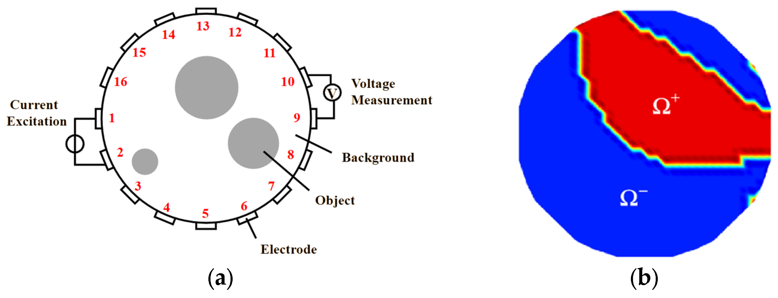
Figure 1. Schematic diagram of ERT current excitation: (a) EIT measuring principle; (b) measurement decomposition.
Mathematics 13 02663 g001
Figure 2. A dataset with four clusters is partitioned into grids and intersecting grids: (a) simulation models; (b) empty field sensitivity; (c) full-field sensitivity.
Mathematics 13 02663 g002
Figure 3. Comparison of S before and after multiplying a coefficient to partial columns of target pixels: (a) respective sum of partial columns in S; (b) respective sum of partial columns by multipling a coefficient.
Mathematics 13 02663 g003
Figure 4. Comparison of reconstructed iamges by S and S′ for a Chinese character “津”: (a) simulation model; (b) sum of sensitivity effecients; (c) reconstruction by S; (d) reconstruction by S′.
Mathematics 13 02663 g004
Figure 5. Schematic diagram of comparison before and after pre-iteration of sensitivity: (a) the sum of the sensitivities before iteration; (b) sum of sensitivity after pre-iteration.
Mathematics 13 02663 g005
Figure 6. Optimal parameter range in both NLP-DM and NLP-TCS: (a) optimal λ value distribution in NLP-DM; (b) optimal iter distribution in NLP-TCS.
Mathematics 13 02663 g006
Figure 7. Measurement system and empty field model of this experiment: (a) EIT measurement system; (b) applied model of empty field.
Mathematics 13 02663 g007
Table 1. Reconstructed images of LBP, NLP-DM, and NLP-TCS in simulations.
ModelMathematics 13 02663 i001Mathematics 13 02663 i002Mathematics 13 02663 i003Mathematics 13 02663 i004Mathematics 13 02663 i005Mathematics 13 02663 i006
LBP ImagingMathematics 13 02663 i007Mathematics 13 02663 i008Mathematics 13 02663 i009Mathematics 13 02663 i010Mathematics 13 02663 i011Mathematics 13 02663 i012Mathematics 13 02663 i013
NLP-DM ImagingMathematics 13 02663 i014Mathematics 13 02663 i015Mathematics 13 02663 i016Mathematics 13 02663 i017Mathematics 13 02663 i018Mathematics 13 02663 i019Mathematics 13 02663 i020
NLP-TCS ImagingMathematics 13 02663 i021Mathematics 13 02663 i022Mathematics 13 02663 i023Mathematics 13 02663 i024Mathematics 13 02663 i025Mathematics 13 02663 i026Mathematics 13 02663 i027
Table 2. Evaluation to LBP, NLP-DM, and NLP-TCS in simulations.
AlgorithmEvaluation MetricsModel IModel IIModel IIIModel IVModel VModel VI
LBPRE0.1710.2880.2740.2830.2340.257
CC0.4770.4170.4210.5020.5500.555
NLP-DMRE0.1200.1740.1670.1590.1350.171
CC0.7360.6710.6930.7930.8160.721
NLP-TCSRE0.0910.1210.1070.1440.1180.176
CC0.7400.7450.7870.8010.8340.745
Table 3. Images reconstructed by LBP, NLP-DM, and NLP-TCS algorithms.
ModelMathematics 13 02663 i028Mathematics 13 02663 i029Mathematics 13 02663 i030Mathematics 13 02663 i031
LBP reconstructionMathematics 13 02663 i032Mathematics 13 02663 i033Mathematics 13 02663 i034Mathematics 13 02663 i035Mathematics 13 02663 i036
NLP-DM reconstructionMathematics 13 02663 i037Mathematics 13 02663 i038Mathematics 13 02663 i039Mathematics 13 02663 i040Mathematics 13 02663 i041
NLP-TCS reconstructionMathematics 13 02663 i042Mathematics 13 02663 i043Mathematics 13 02663 i044Mathematics 13 02663 i045Mathematics 13 02663 i046
Table 4. Evaluation of results of LBP, NLP-DM, and NLP-TCS algorithms.
AlgorithmEvaluation IndexModel 1Model 2Model 3Model 4
LBPRE0.4240.4210.5060.508
CC0.2710.2610.2800.264
NLP-DMRE0.1630.1670.2560.212
CC0.5990.6300.4880.516
NLP-TCSRE0.0540.0610.0830.069
CC0.8310.8660.7760.846
Disclaimer/Publisher’s Note: The statements, opinions and data contained in all publications are solely those of the individual author(s) and contributor(s) and not of MDPI and/or the editor(s). MDPI and/or the editor(s) disclaim responsibility for any injury to people or property resulting from any ideas, methods, instructions or products referred to in the content.