Abstract
Heat stress is one of the main welfare and productivity problems faced by dairy cattle in Mediterranean climates. The main objective of this work is to predict heat stress in livestock from shade-seeking behavior captured by computer vision, combined with some climatic features, in a completely non-invasive way. To this end, we evaluate two soft computing algorithms—Random Forests and Neural Networks—clarifying the trade-off between accuracy and interpretability for real-world farm deployment. Data were gathered at a commercial dairy farm in Titaguas (Valencia, Spain) using overhead cameras that counted cows in the shade every 5–10 min during summer 2023. Each record contains the shaded-cow count, ambient temperature, relative humidity, and an exact timestamp. From here, three thermal indices were derived: the current THI, the previous-night mean THI, and the day-time accumulated THI. The resulting dataset covers 75 days and 6907 day-time observations. To evaluate the models’ performance a 5-fold cross-validation is also used. The results show that both soft computing models outperform a single Decision Tree baseline. The best Neural Network (3 hidden layers, 16 neurons each, learning rate ) reaches an average RMSE of , while a Random Forest (10 trees, depth ) achieves and offers the best interpretability. Daily error distributions reveal a median RMSE of and confirm that predictions deviate less than one hour from observed shade-seeking peaks. Although the dataset came from a single farm, the results generalized well within the observed range. However, the models could not accurately predict the exact number of cows in the shade. This suggests the influence of other variables not included in the analysis (such as solar radiation or wind data), which opens the door for future research.
Keywords:
mathematical modeling; machine learning; soft computing; Random Forests; neural networks; heat stress in livestock; precision livestock farming MSC:
37M05; 68T05; 92B20; 62H30; 62M10; 92D50
1. Introduction
In the context of livestock productivity, mathematical modeling allows for understanding and quantifying the complex interaction of environmental variables and physiological responses. Taking advantage of well-established principles of mathematical analysis and modeling, this work aims to establish a robust mathematical framework that captures the dynamics of Temperature–Humidity Indices and their relationship to animal welfare. This framework not only facilitates a deeper theoretical understanding but also provides the necessary structure to integrate machine learning methodologies. Through this combination, we aim to improve predictive capacity and practical knowledge to improve livestock management in different climatic conditions.
Artificial Intelligence (AI) is a field of Computer Science that focuses on creating systems capable of performing tasks that normally require human intelligence. These systems include a wide range of tasks ranging from learning, perception, or reasoning to problem solving, image recognition, or decision-making. Moreover, machine learning (ML) techniques—supervised, unsupervised, and reinforcement—are now standard tools across science and engineering (such as, for instance, in the Economy [1] or Sport Sciences [2] but also in the case of the livestock sector [3,4]). In this sense, soft computing is the collective term coined by Zadeh (1994) for computational paradigms—fuzzy logic, Neural Networks, evolutionary algorithms, and their hybrids—that trade exactness for robustness and tolerance to uncertainty. Unlike “hard computing” methods based on exact logic, soft computing approaches are designed to handle noisy, incomplete, or vaguely defined data while delivering solutions that are “good enough” for complex real-world problems [5]. Biological processes rarely unfold in the orderly, deterministic manner that traditional computational methods assume but are conditioned by stochastic fluctuations in the environment, sensor noise, and the intrinsic heterogeneity of living organisms. The behavior of dairy cattle is a clear example: even under identical thermal loads, individual cows respond differently, and camera-based counts of shade-seeking animals are unavoidably imprecise. Because soft computing was explicitly conceived to “compute with words, perceptions, and uncertain data”, it offers a natural fit for this problem domain. Techniques such as Random Forests and Neural Networks tolerate incomplete or noisy inputs, capture nonlinear interactions without requiring a fully specified physiological model, and produce approximate—but operationally useful—outputs that can drive real-time management decisions. By leveraging this tolerance to imprecision, soft computing models provide robust, low-cost tools for precision livestock farming, where the objective is not perfect prediction of every individual but reliable, adaptive guidance under biologically variable conditions.
While ML techniques are widely applied in livestock farming, most studies focus on milk production [6], disease prediction [7], or feed optimization [3]. More specifically, behaviour-focused machine learning work on cattle heat stress has so far targeted proxies other than shade seeking. Chapman et al. [8] forecasted the proportion of animals with panting scores using a deep-learning model driven by micro-climate data; Tsai et al. [9] linked drinking-bout frequency, detected with an embedded CNN imaging system, to heat-load indices; Woodward et al. [10] predicted heat stress events from rumen-temperature boluses via a Cubist model. However, no existing approach simultaneously (i) quantifies shade-seeking counts from computer-vision data, (ii) enriches the raw THI with cumulative and night-time indices, and (iii) outputs interpretable, low-latency commands suitable for real-time barn automation-gaps that the present study addresses. Also, few efforts have targeted behavioral responses to environmental stress, such as shade-seeking, despite its critical importance for mitigating heat stress in animals. This paper addresses this gap by developing predictive models adapted for livestock management in Mediterranean regions, which are particularly vulnerable to heat stress. In our case, we will use three well-known algorithms of supervised learning: Random Forest (as a generalization of a Decision Tree, which will be the first) and Neural Networks. Random Forest has a range of applications in livestock farming, such as, for instance, the prediction of milk production [6], disease detection [7], meat quality classification [11], feed optimization [3], fertility and reproduction prediction [12], or environmental health management [13]. Neural Networks have also been widely used in similar contexts (see, for instance, [14,15,16]). Details of these three soft computing algorithms can be found in Section 2.
In this context, a relevant difference between these two types of algorithms (Random Forest and Neural Networks) lies in the concepts of explainability and interpretability. Explainability and interpretability are key concepts when it comes to understanding and trusting models. On the one hand explainability refers to the ability of the model to provide understandable explanations of its behavior and results. In other words, explainability focuses on providing details and reasons about how and why a prediction was produced. On the other hand, interpretability refers to the ease with which a human being can understand the reasons behind a model’s predictions. Figure 1 positions the three algorithms studied—Decision Tree, Random Forest, and Neural Network—along the interpretability–explainability spectrum. Information about interpretability and explainability can be found in [17].
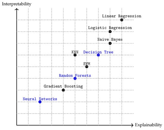
Figure 1.
Relationship between interpretability and explainability of several supervised ML algorithms. The algorithms highlighted in blue are the ones utilized in this study.
We end this first section by talking about the main feature of our dataset (which will be explained at the beginning of the second section): the Temperature–Humidity Index (THI). Mitigating climate change impacts on dairy cattle production systems is essential for the sector’s sustainability, especially as rising temperatures increase the risk of heat stress and negatively impact animal welfare and productivity, particularly in Mediterranean regions. In response, AI integrated with precision livestock farming (PLF) technologies enables detailed analysis of individual data, supporting the adoption and assessment of targeted strategies to reduce heat stress. The THI refers to a measure used to evaluate the combined effects of temperature and humidity on the well-being and performance of animals, particularly livestock, such as dairy cattle, poultry, and pigs. It is commonly used in agriculture and animal husbandry to assess the risk of heat stress, which can significantly impact animal health, productivity, and welfare [18]. Limiting ourselves to such features has multiple benefits in our case: (i) physiological relevance and precedent: The THI is the most widely validated single metric of heat load in dairy cattle; it outperforms raw temperature or humidity and correlates strongly (around ) with rectal temperature, the respiration rate, and milk-yield depression [19,20,21]. Behavioral studies likewise show the shade-seeking probability rising sharply once the THI exceeds 72 [18]; (ii) practical sensor availability: Our aim is an easily deployable decision-support tool. Ambient temperature and humidity are already monitored on most farms at less than EUR 100 per node, whereas pyranometers, anemometers, or infrared thermography entail much higher cost and maintenance. Limiting features to THI-based signals therefore maximizes the real-world uptake; (iii) capturing acute and carry-over heat load: we enrich the raw THI with two derivatives—the day-time accumulated THI (area under the curve) and the previous-night mean THI—to reflect both immediate stress and overnight recovery debt, which existing ML studies seldom include; and (iv) interpretability: keeping three biologically grounded predictors simplifies rule extraction for the downstream fuzzy controller and avoids multicollinearity inflation. To the best of our knowledge, no previous study has forecast dairy-cow heat stress behavior from camera-derived shade-seeking counts combined with THI-based features. Earlier machine learning approaches relied on production traits and environmental sensors rather than behavior [22,23] or used computer vision for other behaviors, such as feeding and rumination [24]. Hence, the present study is the first to deliver a low-latency, behavior-based predictive system for heat stress management. In summary, in this paper, we therefore aim to select the most appropriate AI approach to predict the number of cows in the shade under different THI conditions. To this end, Decision Trees, Random Forest, and Neural Networks will be assessed. Animals exposed to high temperatures often exhibit behavioral adaptations to alleviate thermal discomfort. Among these, seeking shade is a primary response, even preferred over other cooling strategies, like sprinklers or showers. Of course, providing shaded areas can effectively reduce the thermal load on animals, enhancing their comfort and performance. Moreover, a study by Schütz et al. (2010) highlighted that dairy cattle prioritize access to shade under heat stress conditions, underscoring its importance as a mitigation strategy [25].
Our methodology incorporates novel features derived from the raw data, such as the accumulated THI and the previous night’s average THI, to capture both immediate and cumulative effects of heat stress on cow behavior. Additionally, this study is among the first to compare Random Forests and Neural Networks in this context, offering insights into the trade-offs between accuracy and interpretability for real-world farm management. The use of 5-fold cross-validation ensures robust model evaluation, minimizing bias and variance across a limited dataset.
2. Materials and Methods
2.1. Dataset Description, Processing, and Tuning
The dataset for our study originates from a farm located in Titaguas, València in Spain. This farm includes a feedlot with a shaded area in the center, monitored by three cameras that count the number of cows within the shaded area. The dataset consists of observations taken every 5–10 min during the summer of 2023, spanning from 11 July 2023 to 16 October 2023. The observations differ between day and night.
During the day (from 07:00 to 21:00), each observation includes the number of cows in the shade, the temperature (in degrees Celsius), the relative humidity (in percent), and the exact time of observation. As for the night-time (from 21:00 to 07:00), each observation includes the temperature, relative humidity, and the exact time of observation, since the number of cows in the shade is meaningless. Similar to the day-time data, temperature and relative humidity are recorded to track night-time environmental conditions.
From these data, we have derived new variables for use in the models, in addition to the number of cows in the shade and the time. Firstly, the time variable has been transformed into a continuous real value for model training. This transformation allows the model to process time as a numerical feature rather than a categorical one. Secondly, with temperature and relative humidity, we calculate the Temperature–Humidity Index (THI). There are different formulas to calculate the THI depending on the context, the type of animal, and the region (see [26] and the references therein). In our case, the formula we are using, originally proposed by the National Research Council (NRC) in 1971 [27], is
where is the dry bulb temperature in Celsius, and RH is the relative humidity in decimal form. This index serves as a key indicator in our models, quantifying the combined effect of temperature and humidity on the cows’ comfort. Furthermore, we derived two additional variables from the THI: the previous night’s THI, calculated as the average of the previous night, and the accumulated THI, which is the average from the first hour of the day (07:00) up to the current observation time.
The dataset includes the following variables (columns):
- Number of cows in the shade.
- Exact time of observation.
- The current THI.
- The average THI of the previous night.
- The accumulated THI.
As we may expect, pairwise Pearson correlations revealed a strong association between the current THI and the accumulated THI (). Linear variance-inflation diagnostics yielded a value of for the Accumulated THI, whereas the remaining predictors showed VIF smaller than (see Table 1). Although this indicates multicollinearity in a linear setting, tree-based methods are known to be robust to correlated inputs; nevertheless, we provide additional robustness checks in Section 3.

Table 1.
Linear variance-inflation (VIF) of the derived variables.
We restricted the feature space to three THI-based covariates plus the time of day to test a low-cost representation that can be computed on a farm in real-time. We acknowledge that omitting additional environmental—e.g., solar radiation and wind—and individual-level factors—e.g., parity and health status—may limit explanatory power; these will be explored in future extensions.
Initially the data spanned from 11 July 2023 to 16 October 2023, covering a total of 98 days, and we were ultimately left with 75 days of data due to some days not being correctly recorded. This results in a total of 6907 observations. Each day has distinct characteristics or variables, so we employed a cross-validation with 5 folds for model validation. This choice is motivated by several reasons, including the need to assess the model’s performance reliably with a limited dataset and to ensure that the model generalizes well to unseen data (see [28,29]).
For each fold of the cross-validation, we randomly selected of the days (15 days) for testing and used the remaining (60 days) for training the model. Importantly, the test sets form a partition of the total dataset, meaning that for each fold, the test set contains no data from the other test sets. Figure 2 shows a diagram of how this partition is performed. Therefore, the model is trained for each of the 5 folds, using around 5538 observations for training and 1369 for testing on each one.
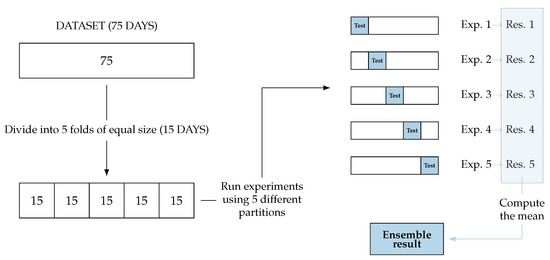
Figure 2.
Cross-validation ensemble: the complete dataset is divided into 5 folds. We run 5 experiments with different partitions (of test and training). Each experiment gives a result. The final result of the ensemble is the mean of the obtained results of the experiments.
For determining the model performance, we use the root mean square error (RMSE). This metric indicates how far the model predictions are from the real data observations, being 0 for perfectly accurate predictions. The RMSE provides an estimate of the number of cows for which the predictions differ from reality. Its formula is
where represents the actual data and represents the corresponding predictions, with N being the test dataset length. Note that when we report this error metric for the entire dataset, it is calculated as the mean of the values across all cross-validation folds.
Regarding preprocessing and tuning the time of day was encoded as a continuous numeric variable. For tree-based models no feature scaling was applied; for the Neural Network, inputs were z-standardized. We excluded days with incomplete logging (resulting in 75 days) and dropped rows with missing predictors during training; no imputation was used for trees. Hyperparameters were selected via 5-fold cross-validation: for the Random Forest we evaluated num.trees and max.depth . The final setting (10 trees, max depth ) achieved a near-optimal error while preserving interpretability.
In the rest of the section, we detail the methods used for model development and validation. It presents the performance metrics and insights from the machine learning models applied to predict the number of cows seeking shade in response to different environmental conditions. Each of these models offers different advantages in terms of accuracy and interpretability (see Section 1), and we will analyze their results to determine the most appropriate approach for this problem. More specifically, we begin examining the Decision Tree, a highly interpretable model that provides valuable insights into the key factors that determine cow behavior. We then move on to Random Forests, which combine multiple Decision Trees to improve prediction accuracy and reduce overfitting. Finally, we will discuss the performance of Neural Networks, which offer a more complex and flexible framework for capturing nonlinear relationships between variables but with less interpretability.
All computations, including data processing, model training, and inference time measurements, were performed on a workstation equipped with an Intel® Core™ i7-12700 CPU @ 2.10 GHz, 32 GB RAM, running Ubuntu 22.04 LTS and Python 3.11 with scikit-learn 1.3.1 and PyTorch 2.1.0. No GPU acceleration was used.
2.2. Soft Computing Decision Tree Algorithm
A Decision Tree is a type of supervised learning algorithm used for both classification and regression tasks. It works by splitting a dataset into smaller subsets according to the possible outcomes that may occur depending on decisions, as shown, for example, in Figure 3. The tree starts at the root node (representing the entire dataset and the first attribute/feature) and splits the data into subsets based on an attribute that maximizes a specific criterion.
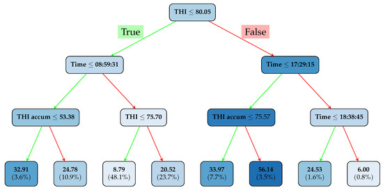
Figure 3.
Decision Tree. The color represents the number of cows in the shade: the more intense the color, the more cows are in the shade that meet these conditions. The values in the terminal nodes are the predictions for the number of cows in the shade, and the percentages indicate the proportion of samples that meet the condition (there are a total of 5538 samples).
Let us explain how the algorithm divides each node [30,31]. Assume that a particular N node has some observations. The predicted value of the model for that node consists of the mean of the values of the observations in it. Then, the training squared error can be computed as
that is, the variance (here is the number of elements on N). However, many points with different values can be in the same node, causing a huge error, so it will be split into two groups (nodes), , where
To achieve this, a variable j and a threshold t must be selected such that the resulting partition creates two new nodes ( and ) with the lowest possible error, minimizing . This process is repeated for each node that contains more observations than a predefined threshold (in our case 2), or when the node reaches a depth greater than a set value, which represents the number of splits from the root node to the current one. The final nodes, which can no longer be split, are called leaves.
Once the tree is trained, that is, all the conditions and thresholds are known, its prediction of a new observation x is computed as follows. The observation starts from the root node and follows the branches according to the conditions satisfied until it arrives at a leaf L. The predicted value for x is , and the mean of all training observations in the node is L.
The deeper the tree and the smaller the allowed nodes (in terms of the minimum number of observations required at each node), the smaller the error in the training set. In the extreme case where each leaf consists of only one observation, the training error will be 0, but this does not mean that the error will be lower when predicting new observations (for example, on the test set). This phenomenon is known as overfitting, and we will see how the selection of hyperparameters is performed to allow the model to be flexible enough to fit the data without being overfitted.
In our particular case the Decision Tree model is particularly well suited for understanding how individual features influence cow behavior, as it visually represents decision rules in a hierarchical structure. This makes it easy to identify the thresholds and conditions under which cows are most likely to seek shade.
In the following, we present the structure of the Decision Tree model applied to our dataset. Figure 3 shows a tree with a depth of 3 for illustrative purposes, offering a clear representation of the key factors involved (current THI, time of day, and THI accumulation). Indeed, as can be seen, the main factor at the root of the tree is the THI, with a threshold value of . This indicates that when the THI exceeds this value, cow behavior changes significantly, with more cows seeking shade.
However, as shown in Table 2, the optimal depth for the Decision Tree model is 5, yielding an RMSE of . This depth level allows the model to capture the complexity of the relationships between the THI, time, and cow behavior without overfitting the data. Interestingly, as the depth increases above 5, the error also begins to increase. This suggests that the model begins to overfit, capturing noise instead of meaningful patterns. Overfitting is a common problem in Decision Trees, especially when the depth is allowed to grow too large, as the model becomes too specific to the training data, losing generalizability. Of course, although deeper models can incorporate more variables, potentially including the THI from the previous night, the lack of relevance in the 3-depth model indicates that immediate environmental conditions play a much more important role in determining cow movements to shaded areas.
Table 2.
Decision Tree errors (RMSE) for different tree depths, ranging from 1 to 50. The model with the lowest error is highlighted in blue.
Although the Decision Tree provides a clear and interpretable model, it may be interesting to explore other methods that capture more complex interactions between variables. This is the purpose of the next types of algorithms.
2.3. Soft Computing Random Forest Algorithm
As the performance of a Decision Tree is limited, an ensemble of many of them can be considered to form a Random Forest—which also works for classification and regression tasks. This method is particularly effective for improving accuracy while mitigating overfitting. The Random Forest is an ensemble of multiple Decision Trees combining the predictions of several base estimators to improve robustness and accuracy. It provides estimates of feature importance, which can help in understanding the underlying structure of the data (see [32,33]). This model is less interpretable compared to a single Decision Tree due to the aggregation of multiple trees and can also be slower to train compared to simpler models, especially with large datasets.
The algorithm works as follows: given an observation x, the output of the Random Forest is given by the mean of the prediction of all Decision Trees in the case of regression or the majority vote in classification (see Figure 4).
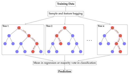
Figure 4.
Random Forest working example.
To avoid having the same tree each time, which would have no improvement when averaging them, some randomness is intentionally introduced on each one, which is usually both included in the training set and the variables used. A fixed number of variables are randomly selected for each tree (three out of four, in our case). Moreover, not all training sets are considered on each tree, with a sample of the training dataset allowing duplicates. This process is known as bootstrapping.
The performance of the Random Forest model is evaluated in comparison to single Decision Trees, focusing on its error reduction capabilities as the number of trees increases and in relation to tree depth. In Figure 5, we observe that the model with a tree depth of 5 (see the green line) achieves the best fit for our dataset, consistent with the optimal depth observed in the Decision Tree model. Note that increasing the depth, while providing a better fit to the data used for building the model, declines the overall performance when tested on unseen data. As the number of trees increases, the error (measured by RMSE) decreases, demonstrating the benefit of using an ensemble of trees. However, beyond 10 trees the error stabilizes, resulting only in marginal gains (around a decrease from 10 to 1000 trees). For this reason, we opted to use a model with 10 trees, which offers a reasonable balance between accuracy and interpretability, achieving an RMSE of .
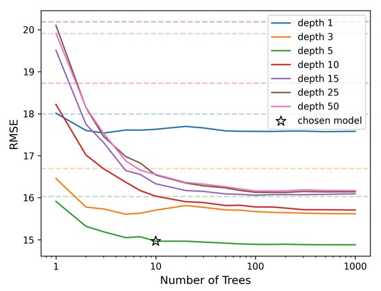
Figure 5.
Random Forest errors (RMSE) for varying numbers of trees (ranging from 1 to 1000) and depths (ranging from 1 to 50). The dashed lines in lighter colors represent the errors of single Decision Trees with corresponding depths, used as a reference for comparison with the Random Forest model. The chosen model, marked with a star, balances accuracy and computational efficiency.
The trade-off between the number of trees and model interpretability is crucial. While more trees generally improve accuracy, especially in complex, high-dimensional datasets, the added complexity can make it harder to interpret the model’s behavior. In our case, using 10 trees allows us to retain a high level of interpretability while achieving near-optimal performance.
2.4. Soft Computing Neural Networks Algorithm
A Neural Network is a model inspired by the human brain’s structure and function. It consists of interconnected layers of nodes (called neurons), as shown in Figure 6, where each connection has a weight that adjusts as learning progresses. It can be used to identify patterns and relationships in data through a training process, but also for classification and regression. During training, the network learns by adjusting weights based on the errors of its predictions compared to known outcomes (see [34,35]). Each layer consists of a linear transformation and a composition with a nonlinear function. The number of layers, the dimensions of each one, and the nonlinear functions used on each are fixed as hyperparameters of the model, while the weights of the linear transformation are optimized on the training.
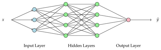
Figure 6.
Scheme of an example of a (Fully Connected) Neural Network. The input x represents the input data, while denotes the model’s prediction. The network consists of an input layer, multiple hidden layers, and an output layer.
During training, backpropagation is used to adjust the network weights. This process consists of calculating the model prediction, , for each observation x in the training dataset and comparing it to the true target, y. If does not coincide with y, the weights are updated to reduce the prediction error. This is achieved using a gradient-based optimization algorithm that minimizes the squared error (SGD or Adam algorithm). Weight updates are propagated backward through the network, layer by layer. Training is repeated for all observations in the training dataset during a fixed number of times, called epochs, or when the error in some test dataset attains a minimum (early stopping parameter). For the best performance of the (Fully Connected) Neural Network (FCNN) model and to avoid variables with larger scales having more influence on the predictions, all variables are scaled so that their mean is 0 and their standard deviation is 1.
Neural Networks are powerful models capable of capturing complex, nonlinear relationships between inputs and outputs. By stacking multiple layers of neurons, these networks can approximate intricate patterns in the data effectively. In the following sections, we will assess the performance of different configurations of the Neural Network. Our focus will be on how factors such as the learning rate, the number of neurons per layer, and the total number of layers influence the predictive accuracy of the model.
There are several activation functions available for use in Neural Networks [36,37]. However, for our FCNN implementation, we have selected the Rectified Linear Unit activation function for hidden layers. This function, mathematically expressed as , allows the network to efficiently model nonlinear relationships in the data. For the output layer, we use a linear activation function defined as . This ensures that the output can take any real value, which is suitable for our prediction task.
The primary challenge when working with Neural Networks lies in determining the optimal architecture—balancing the depth (number of layers), width (number of neurons per layer), and learning rate. While deeper and wider networks have the potential to capture more intricate patterns, they also increase the risk of overfitting and may require significantly more computational resources. Hence, selecting the right configuration is critical to achieving both accuracy and efficiency. To rigorously identify the architecture, 45 different Neural Networks have been tested with all the combinations of these hyperparameters: 1, 3, or 5 layers with 4, 16, 64, 256, or 1024 neurons each, and a learning rate of , , or . All models are trained for 50 epochs to ensure convergence.
Table 3 shows the performance of eight Neural Network models with varying configurations. The results indicate that the most efficient model, in terms of balancing complexity and error, is Model 2, which has 3 hidden layers with 16 neurons in each layer and a learning rate of . This model achieves an RMSE of using only 641 parameters, making it accurate and relatively simple compared to other more complex models. Below, we discuss the key factors that affect the performance of Neural Networks.
Table 3.
Performance of the best error-based models (RMSE) with different learning rates (lr), neurons, and layers. We also show the number of parameters to optimize and the training time (in seconds) of each model. In blue is the best model balancing complexity (number of parameters) and RMSE.
One clear observation from the results is that increasing the number of neurons per layer does not always yield better results. For instance, Model 1, with 5 (hidden) layers and 16 neurons per layer, achieves an RMSE of , comparable to Model 4, which has 64 neurons per layer and a slightly higher error (). This suggests that simpler architectures can perform well, avoiding excessive model intricacy. Additionally, models with fewer layers, such as Model 2 with only 3 layers and 16 neurons per layer, achieve competitive error values, demonstrating that adding more layers may introduce unnecessary complexity without significant performance gains.
Another crucial hyperparameter that affects model performance is the learning rate (lr). In our experiments, we tested different rates: , , and . The results reveal that higher learning rates, such as (Model 7, RMSE ), hinder convergence, while lower rates tend to produce lower error values, especially when used with a smaller number of layers and neurons.
Finally, in the five best configurations, the RMSE values remain in a narrow range between and . Despite the variations in layers, neurons, and learning rates, the best performing models (Models 1 and 2) show very close error values, with a difference of only . Given these minimal differences, we selected Model 2, which has fewer parameters (641) and is therefore more computationally efficient (training time of s) without compromising accuracy. This balance between simplicity and performance makes it an ideal choice for practical applications requiring faster training times and lower resource consumption.
From Figure 7, it is evident that increasing the number of epochs beyond 10 does not significantly improve the model error. After about a decade of epochs, further training offers little to no advantage in terms of predictive accuracy. This insight is particularly relevant for applications requiring instant model recalculations, such as real-time systems, where the model could effectively operate with this number of epochs. This approach allows for greater efficiency in terms of training time and computational resources without significantly affecting the model’s performance. For this reason, we set the number of epochs to 10 for the final model.
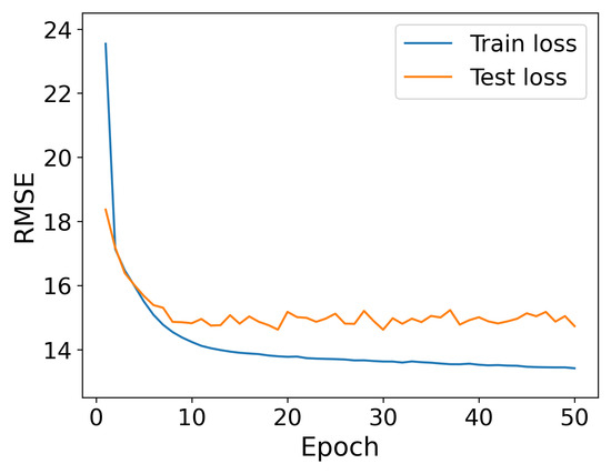
Figure 7.
Evolution of RMSE for Neural Networks over 50 training epochs.
3. Results
3.1. Global Model Performance
We begin by comparing the three machine learning models implemented: Decision Tree with 5 depth, Random Forest consisting of 10 trees all with 5 depth, and a Neural Network with 3 hidden layers of 16 neurons each, learning rate, and trained for 10 epochs. The comparison is given not only in terms of RMSE but also in terms of training time, interpretability, and explainability (see Figure 1).
On the one hand, the Decision Tree model has an RMSE of , which is the highest among the models compared, meaning it is less accurate for prediction. Moreover, the training time of the Decision Tree is extremely low ( s), making it particularly suitable for scenarios where fast model training is essential. However in terms of interpretability, the Decision Tree scores Very High (which means the model is easy to understand), as its structure is simple and intuitive, resembling a flowchart. In a similar way the explainability of the Decision Tree is rated as high, meaning that the decision-making process of the model can be clearly explained, making it easier to trace the reasoning behind predictions.
The Random Forest model has a slightly lower RMSE of , indicating better accuracy compared to the Decision Tree. The training time of the Random Forest model is slightly higher ( s) but still sufficiently fast to be practical in settings requiring frequent model re-training. Its interpretability is rated Medium/High. Although more complex than a single Decision Tree due to the ensemble of trees, it still maintains some interpretability because individual trees can be analyzed. The explainability of the Random Forest model is rated as Medium, as it is harder to fully explain how multiple trees work together in the ensemble, but some level of explanation is still possible.
Finally, the Neural Network model has the lowest RMSE of , making it the most accurate of the three models in terms of predictions. However, this gain in predictive accuracy comes at the cost of a significantly longer training time ( s). Furthermore, the interpretability of this model is low, meaning it is difficult to understand how the model works, due to its complex structure with layers of interconnected neurons. Similarly, the explainability is rated low, as it is challenging to explain how the model arrives at specific predictions, making it a black box in many cases.
This comparison (see Table 4) highlights a trade-off between accuracy (RMSE), interpretability, explainability, and training time: models with better accuracy, like the Neural Network, are harder to interpret, explain, and also require significantly more time to train; conversely, the Decision Tree offers higher interpretability and explainability, with slightly lower accuracy and minimal training time. The Random Forest stands as a compromise between prediction error, model transparency, and computational efficiency.
Table 4.
Comparison of final model using four criteria: training time, RMSE, interpretability and explainability. The preferred model is highlighted in blue.
Finally, permutation-based variable-importance analysis (see Figure 8) confirms that the time of day is by far the dominant predictor: permuting this variable increases the out-of-bag MSE by around . The next two variables are the current THI (around ) and the accumulated day-time THI (around ). In contrast, permuting the night-time mean THI raises the error by only around . Taken together, these results indicate that the model relies primarily on the circadian pattern captured by the time float, while the instantaneous and cumulative day-time heat load provide substantial—but partially overlapping—information. The thermal conditions of the previous night contribute to a lesser extent but still improve performance beyond day-time metrics alone.
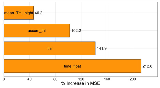
Figure 8.
Permutation importance averaged over the 10 tree, 5 depth Random Forest.
3.2. Error Distribution Analysis
Now, we compare the real and predicted values for the number of animals seeking shade over the span of 75 days. By analyzing the raincloud plot shown in Figure 9, we can draw several conclusions about the model’s performance in terms of RMSE values.
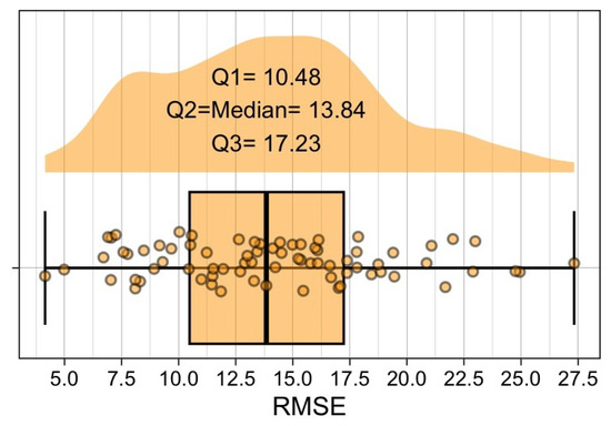
Figure 9.
Raincloud plot representing the distribution of Random Forest errors (RMSE) calculated for each day across each cross-validation partition. The box shows the interquartile range (IQR), with the median error represented by the central line within the box, which is . The whiskers extend to the minimum and maximum RMSE values. Distribution of the days and the first () and third () quartiles are also given.
First, the model’s predictions are generally consistent, as indicated by a median RMSE of . This relatively low median error suggests that the model performs accurately on average. The interquartile range (IQR) of the daily RMSE values (–) represents roughly 57–94% of the average number of cows observed in the shade () and only 13–22% of the full scale of the target variable (0-80). This proportion indicates that most daily prediction errors remain tightly clustered, supporting the description of the error distribution as compact (see Figure 9). Moreover, we assessed the distribution of daily RMSE values: a Shapiro–Wilk test did not reject normality (). We therefore report the median (; bootstrap CI of –) together with the IQR, which confirms that daily errors are tightly concentrated.
Second, the plot reveals a few RMSE values extending toward the extremes (and above 25). This indicates that, in certain cases, the model performs less accurately. These outliers may correspond to specific scenarios or data points where the model struggles to generalize, possibly due to variations in environmental conditions or unmodeled factors. Addressing these cases could involve incorporating additional features or refining the model to improve its generalizability.
Figure 10 summarizes the daily errors of the Random Forest. Applying Tukey’s rule () did not yield any statistical outliers: the dashed line is above the highest observed RMSE. Therefore, we have labeled the top decile of the distribution (orange circles) as days with “high error”. All of these are grouped into a daily average THI above 75, confirming that large deviations only occur under the most severe heat loads and not due to random problems with the data or model instability. The absence of real outliers supports the idea that Random Forest errors behave well throughout the study period, with performance degrading smoothly as heat stress intensifies.
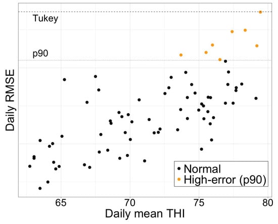
Figure 10.
The daily prediction error (RMSE) plotted against the corresponding daily mean THI. Black circles mark days within the interquartile range; orange circles highlight the upper decile of errors (RMSE ). The dotted horizontal line denotes the threshold, while the dashed line shows the value.
Although no statistical outlier was detected, the day with the single largest error—RMSE , 11 July 2023, Figure 11a—coincided with an afternoon THI peak of . By contrast, the day with the lowest error—RMSE , 15 October 2023, Figure 11b—never exceeded THI and displayed fewer than ten cows in shade throughout the afternoon; the model therefore remained within animals of the observations. Because these high error cases represent only of the evaluation period and cluster in the upper tail of the THI spectrum, their impact on the overall performance metrics is limited, yet they highlight the need for additional features, such as solar-radiation or wind-speed indices—for forecasting under extreme heat.
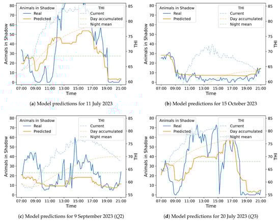
Figure 11.
Random Forest predictions for specific dates corresponding to the maximum (a) and the minimum RMSE values (b), and also to the median (c) and the third quartiles (d). These figures follow the same format as Figure 12.
3.3. Case Studies
Hereafter, we present the real and predicted values for the number of animals in the shade over the course of the day corresponding to the first quartile in terms of that day’s RMSE (18 August 2023), by using our Random Forest algorithm. We also include information about the THI (accumulated day, mean night, and current).
As illustrated in Figure 12, early in the day, from 07:00 until around 11:00, the number of animals in the shade is low, corresponding with lower THI values. Both real and predicted values are similar during this period. Between 11:00 and 17:00, as the current THI increases sharply, there is a remarkable increase in the number of animals seeking shade. This trend is captured well by both the real and predicted data, although the predicted values (orange line) display a smoother, less variable appearance. This effect arises because each tree in the Random Forest makes piecewise-constant predictions over large regions of the input space, and the final output is averaged across multiple trees and cross-validation folds, which naturally smooths out local fluctuations in the data.
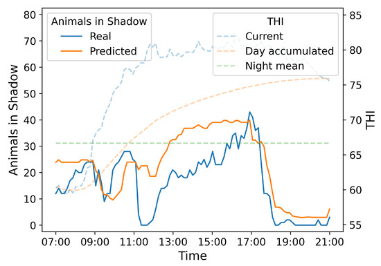
Figure 12.
Random Forest predictions for 18 August 2023, with the day corresponding to . The left Y-axis (with continuous lines) represents the number of animals in the shade (ranging from 0 to 80), the right Y-axis (with dashed lines) indicates the value of the THI (ranging from 55 to 85), and finally, the X-axis displays the time of day (ranging from 07:00 in the morning to 21:00 in the evening). The blue line represents the real data, and the orange line shows the predicted values. Additionally, the dashed blue line represents the current THI, the dashed orange line indicates the accumulated THI throughout the day, and the green dashed line represents the average night-time THI of the previous day.
After 17:00, as the THI decreases, the number of animals in the shade also drops significantly, and both real and predicted values approach zero towards the end of the day. The predictions of the Random Forest model (orange line) follow the general trend of the real data (blue line) reasonably well. However, there are some discrepancies, especially towards midday and early afternoon (from 13:00 to 17:00), where the model slightly overestimates the number of animals in the shade. On the other hand the THI accumulated during the day (dashed orange line) increases throughout the day, reflecting the cumulative heat stress experienced over time. This cumulative THI could have a prolonged impact on animal comfort, contributing to the increased use of shaded areas as animals try to avoid heat stress.
Finally, as we can also see in Figure 11, the prediction model in the three plots (, , and ) follows the general trend but, as expected, the prediction overlooks short-term fluctuations. Particularly, it predicts when more animals move into the shade and when they leave with an accuracy of less than 90 min. Indeed, for each of the 75 days, if we compute the absolute difference between the predicted and the observed time of the daily shade-seeking peak, then the mean absolute deviation is min with a confidence interval of 71.6–133.3 min (t-based CI, ). In addition, of days show an error below 90 min, being the Wilson CI for that proportion of 57.6–79.5%. However, it cannot find the exact number of cows in the shadow area. This fact, may indicate that other factors affect the animals’ decisions, but the time, THI, and accumulated THI at day-time and night-time explain most of its behavior.
4. Discussion
In this work, we have analyzed the performance of three soft computing machine learning models—Decision Trees, Random Forests, and Neural Networks—to predict the number of cows seeking shade as a response to varying environmental conditions. Using data from a farm in Titaguas, Valencia, the research aimed to determine which model could best predict shade-seeking behavior in response to the Temperature–Humidity Index (THI), a key indicator of thermal stress in cattle, while also exploring the capabilities and limitations of these models for livestock management under heat stress conditions.
The results have shown that each model has distinct strengths. Neural Networks provided the highest accuracy, with a root mean square error (RMSE) of , followed closely by the Random Forest at and the Decision Tree at . However, model performance was not evaluated solely based on accuracy. Interpretability and explainability were also central to the evaluation, especially for practical applications in farm management. Although the Decision Tree model is the most interpretable (given its flowchart structure that allows direct analysis of how different variables influence predictions), Random Forests, while more complex, retain some interpretability as individual trees can be analyzed to understand decision pathways. In contrast, Neural Networks, despite their high accuracy, were the least interpretable due to their multi-layered structure, often referred to as a black box in machine learning.
Taking these factors into account, Random Forests has been chosen as the optimal model, offering a balance between accuracy, interpretability, and explainability. It has effectively captured overall trends in cow movement patterns, accurately predicting when cows would seek or leave shaded areas within a 90 min precision in most instances. This precision is important in real-world applications, where timely interventions can help mitigate the effects of heat stress.
The performance gap between the Random Forest model and the Neural Network is small (around RMSE), yet the tree-based ensemble is far easier to interpret and is inherently robust to noisy or missing inputs—an essential property in commercial farms where cameras may be hidden and low-cost sensors drift over time. This robustness makes the model an ideal upstream component for a hybrid soft-computing controller: its predicted shade-seeking count can feed a fuzzy logic rule base that activates fans, sprinklers, or retractable awnings, according to linguistic rules, such as “if THI is high and Predicted Shade is many, then increase airflow”. In practice, the Random Forest supplies a single scalar output—the predicted number of cows expected to occupy the shade 15 min ahead. That value is fuzzified into three linguistic levels (LOW, MEDIUM, HIGH) using the 33rd and 66th percentiles of the training distribution as thresholds. A compact rule base then maps each level to a management action, e.g., IF Predicted Shade = HIGH THEN set ventilation to level 2; IF Predicted Shade = MEDIUM THEN level 1; ELSE keep fans off. This one-to-one conversion—scalar → fuzzy label → actuation rule—keeps the controller transparent while retaining the data-driven accuracy of the forest.
In this article, several variables influencing shade-seeking behavior have been identified: in particular, the time of day, current THI, and cumulative THI throughout the day and night. These factors strongly correlated with the cows’ movement towards or away from shaded areas, underscoring their relevance in managing thermal stress. Although our feature set is intentionally minimal—THI plus time—real-world implementation across locations will benefit from additional covariates (global solar radiation, wind speed, shade capacity, stocking density). Furthermore, as part of the European Re-Livestock consortium, this study can be replicated on farms in other climates, allowing us to test alternative THI formulations used in different regions. These steps will help turn the current prototype into a multi-site decision-support tool. Beyond our single-site study, we will conduct external validation across contrasting farms and seasons (leave-one-farm-out), improve portability via site-specific quantile recalibration of decision thresholds and light fine-tuning on a small local subset, and monitor concept drift with scheduled re-training as datasets scale.
However, some limitations have also been identified. The models struggled to accurately predict the exact number of cows under shade, suggesting that other variables not included in this study may also influence this behavior. Future research could explore these additional factors to enhance model performance.
Finally, we would like to point out that this work focuses on modeling and validation aspects; operational integration—sensor status monitoring, latency budgets, and user interface—is highly site-specific and requires prospective trials on farms that exceed the scope of this study. Given the sampling rate of 5 to 10 min and inference in less than a second on commercial hardware, computational latency is not expected to be limiting; we leave the full details of implementation to a follow-up implementation study.
5. Conclusions
This study demonstrates the potential of using soft computing approaches for mathematical modeling of noisy and highly variable biological behaviors. Using only climatic measurements and camera counts, both Random Forests and Neural Networks accurately predicted the number of dairy cows seeking shade during Mediterranean summer heat waves. The main conclusions are as follows:
- Early warning capability: The models anticipate shade-seeking peaks within one hour, with a median daily RMSE of cows.
- Interpretability: A 10-tree Random Forest (depth ) achieves an average RMSE of while retaining a transparent rule structure, making it the recommended choice for on-farm deployment.
- Minimal feature set: Three easily derived thermal features—the current THI, the accumulated day-time THI, and the mean night-time THI—are sufficient for a low-cost decision-support system that can trigger ventilation, sprinkling, or shading strategies in real-time.
These results show that soft computing models provide robust, affordable tools for precision livestock management aimed at mitigating heat stress and safeguarding animal welfare.
Limitations and External Validation
The limitations and external validation of this paper are as follows:
- Explicit statement of scope: The present dataset represents one Mediterranean region—Titaguas, Spain—during a single summer—June–September 2023. As such, it does not include colder seasons, other housing layouts (as, for instance, composting barns) or different breeds, nor does it capture climatic extremes, such as monsoonal humidity or continental heat waves. While the model performs well on the source farm, its generalizability beyond Mediterranean summer conditions remains to be demonstrated.
- Potential sources of bias:
- (i)
- Management practices: Shade availability, stocking density, and cooling protocols vary widely across farms; these factors could shift the threshold at which cows seek shade.
- (ii)
- Regional weather patterns: Diurnal THI dynamics in arid or tropical zones differ from those in Mediterranean climates, possibly altering the relative importance of the accumulated vs. the instantaneous THI.
- Need for external validation: Future work will involve external validation on at least three additional farms. Following the guidelines of Steyerberg [38], we will report calibration curves and domain-transfer metrics.
- Practical field applications: Finally, the current work stops short of detailing real-time deployment aspects—such as latency budgeting, sensor-fault mitigation, and farmer-oriented user interfaces—because its primary aim is the methodological proof-of-concept. Although preliminary benchmarks show the full inference pipeline runs on basic CPUs in a short time and relies only on readily available temperature and humidity inputs, these engineering questions will be tackled in a dedicated follow-up field study.
Author Contributions
Conceptualization, S.S., D.A.M., R.A., J.M.C., X.D.d.O.A. and F.E.; methodology, S.S., R.A. and J.M.C.; software, S.S., R.A. and D.A.M.; validation, S.S., R.A., D.A.M. and J.M.C.; formal analysis, S.S., R.A. and J.M.C.; investigation, S.S., D.A.M., R.A., J.M.C., X.D.d.O.A. and F.E.; resources, J.M.C. and F.E.; data curation, D.A.M., X.D.d.O.A. and F.E.; writing—original draft preparation, S.S., R.A. and J.M.C.; writing—review and editing, D.A.M., X.D.d.O.A. and F.E.; visualization, S.S., R.A. and J.M.C.; supervision, J.M.C. and F.E.; project administration, J.M.C. All authors have read and agreed to the published version of the manuscript.
Funding
The research of J.M.C. was funded by the Agencia Estatal de Investigación, grant number PID2022-138328OB-C21. The research of R.A. was funded by the Universitat Politècnica de València, Programa de Ayudas de Investigación y Desarrollo (PAID-01-21). The research of D.A.M. was supported by R+D+i project TED2021-130759B-C31, funded by MCIN/AEI/10.13039/501100011033/ and by the “European Union NextGenerationEU/PRTR”. This work has received funding from the European Union’s Horizon Europe research and innovation program under the grant agreement No. 01059609 (Re-Livestock project).
Data Availability Statement
The data presented in this study are not publicly available due to privacy concerns. All the algorithms presented in this paper are available in a GitHub repository and can be accessed at the following link: https://github.com/serjj99/CowShadeSeeking.git (accessed on 14 August 2025).
Acknowledgments
The authors acknowledge the technicians of the Titaguas farm, València, for their valuable help in the animal management during the research activities.
Conflicts of Interest
The authors declare no conflicts of interest.
References
- Calabuig, J.M.; Falciani, H.; Sánchez-Pérez, E.A. Dreaming machine learning: Lipschitz extensions for reinforcement learning on financial markets. Neurocomputing 2020, 398, 172–184. [Google Scholar] [CrossRef]
- Arnau Notari, A.R.; Calabuig, J.M.; Catalan, C.; Garcia Raffi, L.M.; Pardo Gila, J.; Pons Anaya, R.; Sánchez Pérez, E. Using neural networks and hierarchical cluster analysis to study goal kicks in football. Int. J. Sport. Sci. Coach. 2024, 19, 1723–1737. [Google Scholar] [CrossRef]
- Akintan, O.; Gebremedhin, K.G.; Uyeh, D.D. Animal Feed Formulation—Connecting Technologies to Build a Resilient and Sustainable System. Animals 2024, 14, 1497. [Google Scholar] [CrossRef]
- Slob, N.; Catal, C.; Kassahun, A. Application of machine learning to improve dairy farm management: A systematic literature review. Prev. Vet. Med. 2021, 187, 105237. [Google Scholar] [CrossRef]
- Zadeh, L. Soft computing and fuzzy logic. IEEE Softw. 1994, 11, 48–56. [Google Scholar] [CrossRef]
- Ji, B.; Banhazi, T.; Phillips, C.J.; Wang, C.; Li, B. A machine learning framework to predict the next month’s daily milk yield, milk composition and milking frequency for cows in a robotic dairy farm. Biosyst. Eng. 2022, 216, 186–197. [Google Scholar] [CrossRef]
- Luo, W.; Dong, Q.; Feng, Y. Risk prediction model of clinical mastitis in lactating dairy cows based on machine learning algorithms. Prev. Vet. Med. 2023, 221, 106059. [Google Scholar] [CrossRef] [PubMed]
- Chapman, N.H.; Chlingaryan, A.; Thomson, P.C.; Lomax, S.; Islam, M.A.; Doughty, A.K.; Clark, C.E.F. A Deep Learning Model to Forecast Cattle Heat Stress. Comput. Electron. Agric. 2023, 211, 107932. [Google Scholar] [CrossRef]
- Tsai, Y.C.; Hsu, J.T.; Ding, S.T.; Rustia, D.J.A.; Lin, T.T. Assessment of Dairy Cow Heat Stress by Monitoring Drinking Behaviour Using an Embedded Imaging System. Biosyst. Eng. 2020, 199, 97–108. [Google Scholar] [CrossRef]
- Woodward, S.J.R.; Edwards, J.P.; Verhoek, K.J.; Jago, J.G. Identifying and Predicting Heat Stress Events for Grazing Dairy Cows Using Rumen Temperature Boluses. JDS Commun. 2024, 5, 431–435. [Google Scholar] [CrossRef]
- Shirzadifar, A.; Miar, Y.; Plastow, G.; Basarab, J.; Li, C.; Fitzsimmons, C.; Riazi, M.; Manafiazar, G. A machine learning approach to predict the most and the least feed–efficient groups in beef cattle. Smart Agric. Technol. 2023, 5, 100317. [Google Scholar] [CrossRef]
- Hempstalk, K.; McParland, S.; Berry, D. Machine learning algorithms for the prediction of conception success to a given insemination in lactating dairy cows. J. Dairy Sci. 2015, 98, 5262–5273. [Google Scholar] [CrossRef]
- Valletta, J.J.; Torney, C.; Kings, M.; Thornton, A.; Madden, J. Applications of machine learning in animal behaviour studies. Anim. Behav. 2017, 124, 203–220. [Google Scholar] [CrossRef]
- Grzesiak, W.; Błaszczyk, P.; Lacroix, R. Methods of predicting milk yield in dairy cows—Predictive capabilities of Wood’s lactation curve and artificial neural networks (ANNs). Comput. Electron. Agric. 2006, 54, 69–83. [Google Scholar] [CrossRef]
- Naqvi, S.A.; King, M.T.M.; Matson, R.D.; DeVries, T.J.; Deardon, R.; Barkema, H.W. Mastitis detection with recurrent neural networks in farms using automated milking systems. Comput. Electron. Agric. 2022, 192, 106618. [Google Scholar] [CrossRef]
- Lin, D.; Kenéz, Á.; McArt, J.A.A.; Li, J. Transformer neural network to predict and interpret pregnancy loss from activity data in Holstein dairy cows. Comput. Electron. Agric. 2023, 205, 107638. [Google Scholar] [CrossRef]
- Molnar, C. Interpretable Machine Learning, 2nd ed.; Independently Published, 2022; Available online: https://christophm.github.io/interpretable-ml-book (accessed on 14 August 2025).
- Polsky, L.; von Keyserlingk, M.A. Invited review: Effects of heat stress on dairy cattle welfare. J. Dairy Sci. 2017, 100, 8645–8657. [Google Scholar] [CrossRef]
- West, J.W. Effects of Heat Stress on Production in Dairy Cattle. J. Dairy Sci. 2003, 86, 2131–2144. [Google Scholar] [CrossRef]
- Berman, A. Indices for Environmental Heat Stress. Int. J. Biometeorol. 2005, 49, 189–196. [Google Scholar] [CrossRef]
- Dikmen, S.; Hansen, P.J. Is the Temperature–Humidity Index the Best Indicator of Heat Stress in Dairy Cattle? J. Dairy Sci. 2009, 92, 109–116. [Google Scholar] [CrossRef]
- Bovo, M.; Agrusti, M.; Benni, S.; Torreggiani, D.; Tassinari, P. Random Forest Modelling of Milk Yield of Dairy Cows under Heat Stress Conditions. Animals 2021, 11, 1305. [Google Scholar] [CrossRef]
- Becker, C.A.; Aghalari, A.; Marufuzzaman, M.; Stone, A.E. Predicting Dairy Cattle Heat Stress Using Machine Learning Techniques. J. Dairy Sci. 2021, 104, 501–524. [Google Scholar] [CrossRef]
- Guarnido-Lopez, P.; Pi, Y.; Tao, J.; Mendes, E.D.M.; Tedeschi, L.O. Computer vision algorithms to help decision-making in cattle production. Anim. Front. 2025, 14, 11–22. [Google Scholar] [CrossRef]
- Schütz, K.E.; Rogers, A.R.; Cox, N.R.; Webster, J.R.; Tucker, C.B. Dairy cattle prefer shade over sprinklers: Effects on behavior and physiology. J. Dairy Sci. 2011, 94, 273–283. [Google Scholar] [CrossRef] [PubMed]
- Habeeb, A.A.; Gad, A.; Atta, M.A.A. Temperature-Humidity Indices as Indicators to Heat Stress of Climatic Conditions with Relation to Production and Reproduction of Farm Animals. Int. J. Recent Adv. Biotechnol. 2018, 1, 35–50. [Google Scholar] [CrossRef]
- Committee on Physiological Effects of Environmental Factors on Animals; Agricultural Board; National Research Council. A Guide to Environmental Research on Animals; National Academy of Sciences: Washington, DC, USA, 1971. [Google Scholar]
- Kohavi, R. A Study of Cross-Validation and Bootstrap for Accuracy Estimation and Model Selection; Morgan Kaufman Publishing: Burlington, MA, USA, 1995. [Google Scholar]
- Stone, M. Cross-validatory choice and assessment of statistical predictions. J. R. Stat. Soc. Ser. B (Methodol.) 1974, 36, 111–133. [Google Scholar] [CrossRef]
- Quinlan, J.R. C4.5: Programs for Machine Learning; Morgan Kaufmann: Burlington, MA, USA, 1993. [Google Scholar]
- Safavian, S.R.; Landgrebe, D. A survey of decision tree classifier methodology. IEEE Trans. Syst. Man, Cybern. 1991, 21, 660–674. [Google Scholar] [CrossRef]
- Breiman, L. Random forests. Mach. Learn. 2001, 45, 5–32. [Google Scholar] [CrossRef]
- Liaw, A.; Wiener, M. Classification and regression by Random Forest. R News 2002, 2, 18–22. [Google Scholar]
- Goodfellow, I.; Bengio, Y.; Courville, A. Deep Learning; MIT Press: Cambridge, MA, USA, 2016. [Google Scholar]
- LeCun, Y.; Bengio, Y.; Hinton, G. Deep learning. Nature 2015, 521, 436–444. [Google Scholar] [CrossRef] [PubMed]
- Apicella, A.; Donnarumma, F.; Isgrò, F.; Prevete, R. A survey on modern trainable activation functions. Neural Netw. 2021, 138, 14–32. [Google Scholar] [CrossRef] [PubMed]
- Sharma, S.; Sharma, S.; Athaiya, A. Activation functions in neural networks. Towards Data Sci. 2017, 6, 310–316. [Google Scholar] [CrossRef]
- Steyerberg, E.W. Clinical Prediction Models, 2nd ed.; Chapter Model Validation and Updating; Springer: Berlin/Heidelberg, Germany, 2019. [Google Scholar]
Disclaimer/Publisher’s Note: The statements, opinions and data contained in all publications are solely those of the individual author(s) and contributor(s) and not of MDPI and/or the editor(s). MDPI and/or the editor(s) disclaim responsibility for any injury to people or property resulting from any ideas, methods, instructions or products referred to in the content. |
© 2025 by the authors. Licensee MDPI, Basel, Switzerland. This article is an open access article distributed under the terms and conditions of the Creative Commons Attribution (CC BY) license (https://creativecommons.org/licenses/by/4.0/).