Article

Dynamic Portfolio Optimization Using Information from a Crisis Indicator

Department of Mathematics, Technical University of Munich, 85748 Munich, Germany
*
Author to whom correspondence should be addressed.
Mathematics 2025, 13(16), 2664; https://doi.org/10.3390/math13162664
Submission received: 28 July 2025 / Revised: 14 August 2025 / Accepted: 16 August 2025 / Published: 19 August 2025
(This article belongs to the Special Issue Latest Advances in Mathematical Economics)

Abstract

Investors face the challenge of how to incorporate economic and financial forecasts into their investment strategy, especially in times of financial crisis. To model this situation, we consider a financial market consisting of a risk-free asset with a constant interest rate as well as a risky asset whose drift and volatility is influenced by a stochastic process indicating the probability of potential market downturns. We use a dynamic portfolio optimization approach in continuous time to maximize the expected utility of terminal wealth and solve the corresponding HJB equations for the general class of HARA utility functions. The resulting optimal strategy can be obtained in closed form. It corresponds to a CPPI strategy with a stochastic multiplier that depends on the information from the crisis indicator. In addition to the theoretical results, a performance analysis of the derived strategy is implemented. The specified model is fitted using historic market data and the performance is compared to the optimal portfolio strategy obtained in a Black–Scholes framework without crisis information. The new strategy clearly dominates the BS-based CPPI strategy with respect to the Sharpe Ratio and Adjusted Sharpe Ratio.

1. Introduction

Dynamic portfolio optimization problems for various types of investors have been studied extensively in the literature. Since [1], the frameworks have been adapted in many ways to extend the problem, in particular, to make the setting more realistic. The question of how to incorporate economic and financial market forecasts into the portfolio optimization process is of fundamental importance for portfolio managers. However, this aspect has not been discussed widely in the literature. In this article, we present a market model that allows for the incorporation of a crisis indicator in the optimization process. Using the results from [2], we contribute to the literature on dynamic portfolio optimization in market models with stochastic coefficients that are not directly observable.
With respect to the modeling of crisis periods, Markov-switching models are especially discussed in the literature. Evidence for the existence of different market regimes in equity and currency markets is, e.g., in [3]. Portfolio optimization results in Markov-switching models can be found, e.g., in [4,5]. Ref. [6] uses model predictive control for dynamic portfolio optimization based on forecasts of the mean and variance of financial returns resulting from a hidden Markov model with time-varying parameters. Ref. [7] analyzes a defaultable market with parameters depending on the market regime given by a Markov process. Ref. [8] empirically indicates an outperformance of portfolio optimization based on a Markov-switching model compared to a BS framework together with significantly reduced risk measures. To the best of our knowledge, it is only possible to derive closed-form solutions if the Markov-switching regimes are observable. In reality, however, these regimes are often not observable, but they can be estimated. Ref. [9] uses economic variables to estimate regimes for use in asset allocation. The use and impact of regime-switching models is presented in [10,11], which use observations in directional changes to identify normal and abnormal market regimes. In [2], three different market phases are identified and a model is constructed to forecast probabilities for each market phase.
Besides Markov-switching models, portfolio optimization in a large variety of models with stochastic factors is studied in the literature. Ref. [12] examines a continuous-time portfolio optimization problem with a stochastic factor influencing the drift and volatility of the risky asset, with a monotone mean–variance functional as a preference criterion using a differential game approach. Ref. [13] uses asymptotic approximations for the value functions and optimal strategy to maximize utility in a market with two stochastic factors influencing drift and volatility. Portfolio optimization results using stochastic models can be found for the Wishart model in [14] and in [15] for power and logarithmic utility. Results for affine models for the power utility can be found in [16] with jumps and stochastic volatility, as well as for constant relative risk aversion and a quadratic framework in [17]. Especially interesting is the case in [18] of a one-dimensional Heston model with stochastic volatility for the power utility, as our model will cover this model in a simplified special case, with the difference being that, in our model, the stochastic factor influences not only the volatility but also the drift term. The combination of Markov-switching parameters with stochastic factors in a very flexible model is studied for the power utility in [19].
Due to the lack of closed-form solutions for portfolio optimization problems with hidden Markov-switching models, we use a different market model approach. Our model is related to the very flexible framework of [20], but we do not consider Markov switching. Instead, we introduce a stochastic factor that includes transformed market forecasts according to [2]. Within this framework, we show that the resulting strategy is a generalization of a CPPI strategy, which was introduced in [21,22] and allows for an easy implementation. Thus, we contribute to the literature on portfolio optimization in markets with stochastic coefficients, while we also contribute to the literature on forecasting of market regimes by illustrating possible applications of crisis indicators.
The article is structured in the following way. In Section 2, we construct our model for the financial market, with a risky asset whose drift and volatility is influenced by a stochastic factor that represents the transformed forecasted probability of a crisis and is modeled by a Cox–Ingersoll–Ross process. We leave a certain flexibility to the model and prove for certain cases the unique existence of a strong solution for the SDEs of the involved processes. In Section 3, we introduce the continuous-time dynamic portfolio optimization problem. We maximize the expected utility from terminal wealth based on the general class of HARA utility functions. We solve the associated HJB equations and verify the optimality of the derived closed-form solution. In Section 4, we analyze the performance of the strategy compared to the optimal CPPI strategy resulting from the Black–Scholes (BS) framework, which does not take different market phases into account. For this, we fit the Cox–Ingersoll–Ross model of the stochastic factor to the crisis probability forecasts resulting from the approach in [2] and estimate the parameters of our model. The goodness of fit of the resulting model is compared to the BS model. As a last step, the optimal strategy is compared to the optimal BS-based strategy for different risk-aversion parameters of the utility function and different guaranteed floors. Finally, we conclude in Section 5.

2. Model Formulation

We model our financial market using a risk-free asset with constant interest rate r as well as a risky asset, which can also be interpreted as an index or portfolio of risky assets.

2.1. Model Dynamics

The drift and volatility of the risky asset shall depend on the state of the market, which we characterize by the probability of a rough market as opposed to a calm market. Depending on the application, a rough market may in particular be associated with a crisis. We define a stochastic process that depends on this probability to be included in our model definition.
Definition 1. 
We consider the process ( p ( t ) ) t 0 [ 0 , 1 ] as a process that indicates, at every time point t 0 , the probability of having a rough market.
Next, we want to build a market indicator that we can model using the CIR model. For this, we transform ( p ( t ) ) t 0 to be in [ 0 , ) .
Definition 2. 
We consider a market indicator ( X ( t ) ) t 0 defined as
X ( t ) = log ( p ( t ) ) .
Remark 1. 
Note that ( X ( t ) ) t 0 decreases when the probability of having a crisis increases and increases otherwise. Thus, low values indicate a high crisis probability and high values indicate a low crisis probability. As we have X ( t ) [ 0 , ) t 0 , we characterize ( X ( t ) ) t 0 as a mean-reverting CIR process with mean-reversion level θ > 0 and mean-reversion speed κ > 0 .
In the following definition, we specify our financial market model.
Definition 3. 
We assume the following dynamics for the risk-free asset ( P 0 ( t ) ) t 0 , the risky asset ( P 1 ( t ) ) t 0 and the market indicator ( X ( t ) ) t 0 :
d P 0 ( t ) = P 0 ( t ) r d t d P 1 ( t ) = P 1 ( t ) r + μ C + X ( t ) Ψ X ( t ) d t + σ C + X ( t ) Ψ X ( t ) d W P ( t ) = : P 1 ( t ) μ P 1 ( X , t ) d t + σ P 1 ( X , t ) d W P ( t ) , d X ( t ) = κ θ X ( t ) d t + σ ^ X ( t ) d W X ( t ) = : μ X ( X , t ) d t + σ X ( X , t ) d W X ( t )
d W P , W X ( t ) = ρ d t ,
with correlated Brownian motions W P and W X , κ > 0 , σ > 0 , σ ^ > 0 , μ > 0 , C 0 and ρ [ 1 , 1 ] , and where Ψ ( x ) is a general function defined on [ 0 , ) such that ( P 1 ( t ) ) t 0 has a strong solution. (Our model includes the influence of the stochastic market indicator on both drift and volatility. It also reflects a stochastic market price of risk of λ ( t ) = μ σ 2 Ψ ( X ) ).
The last line indicates the assumption that the Brownian motions W P and W X have correlation ρ [ 1 , 1 ] .
Remark 2. 
For the special case C = 0 , we obtain the dynamics
d P 0 ( t ) = P 0 ( t ) r d t d P 1 ( t ) = P 1 ( t ) r + μ X ( t ) Ψ X ( t ) d t + σ X ( t ) Ψ X ( t ) d W P ( t ) d X ( t ) = κ θ X ( t ) d t + σ ^ X ( t ) d W X ( t ) , d W P , W X ( t ) = ρ d t ,
with κ > 0 , θ > 0 , σ ^ > 0 and ρ [ 1 , 1 ] . Note that the choice Ψ ( x ) 1 corresponds to a Heston model where the excess drift is given by μ X ( t ) .
In the following section, we examine the existence of a strong solution for ( P 1 ( t ) ) t 0 . We therefore restrict Ψ ( x ) in such a way that the existence of a unique strong solution is ensured.

2.2. Existence of a Strong Solution for the Model

As σ X ( x , t ) in (3) is not Lipschitz-continuous, we cannot apply common techniques to show the unique existence of a strong solution (see, e.g, Theorem 2.45, pp. 36 f. in [23]). Therefore, we prove pathwise uniqueness using Theorem 1 from [24] and weak existence using Theorem 6.2.4, pp. 65 in [25]. The existence of a unique strong solution then follows with Corollary 3.23, pp. 310 f. in [26].
To show pathwise uniqueness under certain conditions on μ X ( x , t ) and σ X ( x , t ) , we can use Theorem 1 from [24]. The CIR model, which is best known for its role as a short-rate model, has an affine term structure as stated in [27], pp. 68 f. This means that we have an affine exponential structure for the expression (this is one reason for us to use the CIR model, as we will have a similar structure resulting from the Feynman–Kac theorem. This result enables us to use an affine exponential structure for the ansatz to obtain the corresponding solution).
E exp t T X ( s ) d s | F t = exp A ( t , T ) + B ( t , T ) X ( t ) .
Using Theorem 1 from [24] directly on the multi-dimensional process ( P 1 ( t ) , X ( t ) ) t 0 is not possible as the diffusion term of ( P 1 ( t ) ) t 0 depends on ( X ( t ) ) t 0 . There is a more general multi-dimensional version of this Yamada–Watanabe theorem in [28] but, in that version, the square-root in σ X ( x , t ) does not meet the necessary conditions, so it is also not applicable to this case. However, Theorem 1 from [24] can be applied to show the existence of a unique strong solution for the CIR process ( X ( t ) ) t 0 . We can use this fact to argue that, under certain conditions, the existence of a unique strong solution for ( P 1 ( t ) ) t 0 follows. For P ^ 1 ( t ) = ln ( P 1 ( t ) ) , we obtain, using Itô’s formula,
d P 0 ( t ) = P 0 ( t ) r d t d P ^ 1 ( t ) = r + μ C + X ( t ) Ψ X ( t ) 1 2 σ 2 C + X ( t ) Ψ X ( t ) 2 d t + σ C + X ( t ) Ψ X ( t ) d W P ( t ) = : μ P ^ 1 ( X , t ) d t + σ P ^ 1 ( X , t ) d W P ( t ) d X ( t ) = κ θ X ( t ) d t + σ ^ X ( t ) d W X ( t ) = : μ X ( X , t ) d t + σ X ( X , t ) d W X ( t ) d W P , W X ( t ) = ρ d t .
Using the existence of a unique strong solution for X ( t ) , as well as the first two moments of the CIR process, the following lemma can be easily shown.
Lemma 1. 
The process ( P 1 ( t ) ) t 0 has a unique strong solution if μ P ^ 1 ( x , t ) and σ P ^ 1 ( x , t ) fulfill the growth condition
μ P ^ 1 ( x , t ) a + b | x |
σ P ^ 1 ( x , t ) a + b | x |
for some a , b R .
We now show that the assumption of Lipschitz-continuous functions μ P ^ 1 ( x , t ) and σ P ^ 1 ( x , t ) in x implies the growth condition and thus also ensures a unique strong solution, as this is the property that we use for one possible choice of model later.
Lemma 2. 
Let Ψ ( x ) be such that μ P ^ 1 ( x , t ) and σ P ^ 1 ( x , t ) are Lipschitz-continuous in x and | Ψ ( 0 ) | < . Then, P 1 ( t ) has a unique strong solution.
Proof. 
Using that μ P ^ 1 ( x , t ) and σ P ^ 1 ( x , t ) are Lipschitz-continuous in x with Lipschitz constants L 1 < and L 2 < , respectively, it is easy to show that both also fulfill the growth conditions, with
a = max { | μ P ^ 1 ( 0 , t ) | , | σ P ^ 1 ( 0 , t ) | } < and b = max { L 1 , L 2 } < .
These results give us the opportunity to specify the function Ψ ( x ) (the Lipschitz continuity allows us to remain flexible with the choice for Ψ ( X ) while ensuring that the growth conditions are fulfilled for μ and σ to prove the existence of a strong solution with standard techniques), where we consider specifically the following two examples.
Example 1. 
We choose Ψ ( x ) = ( C + x ) l with l , 0 and C > 0 . For this choice, the dynamics of the assets are given by
d P 0 ( t ) = P 0 ( t ) r d t d P 1 ( t ) = P 1 ( t ) r + μ C + X ( t ) l + 1 d t + σ ( C + X ( t ) ) l + 1 2 d W P ( t ) d X ( t ) = κ θ X ( t ) d t + σ ^ X ( t ) d W X ( t ) , d W P , W X ( t ) = ρ d t .
We can show the Lipschitz continuity of μ P ^ 1 ( x , t ) and σ P ^ 1 ( x , t ) in x, leading to the existence of a unique strong solution through Lemma 2. Hence, P 1 ( t ) has a unique strong solution.
Example 2. 
We choose Ψ ( x ) = log ( 1 + x ) x . Here, the model evolves according to
d P 0 ( t ) = P 0 ( t ) r d t d P 1 ( t ) = P 1 ( t ) r + μ log ( 1 + X ( t ) ) d t + σ log ( 1 + X ( t ) ) X ( t ) d W P ( t ) d X ( t ) = κ θ X ( t ) d t + σ ^ X ( t ) d W X ( t ) , d W P , W X ( t ) = ρ d t .
In this case, the Lipschitz continuity of μ P ^ 1 ( x , t ) and σ P ^ 1 ( x , t ) in x is not fulfilled, but it can be shown that the growth condition from Lemma 1 is fulfilled, which also leads to the existence of a unique strong solution.
Remark 3. 
The motivation for these expressions of Ψ ( x ) for the respective cases is that they allow us to replicate some general market dynamics with respect to crisis situations. The chosen general form in the model formulation from Definition 3 allows for the derivation of an optimal portfolio in Section 3. Therefore, we use Ψ ( x ) to give the desired characteristics to the model. As described in [2], crisis situations (when x is small) often come with a low drift and high volatility, while calm periods (when x is big) typically have a high drift and low volatility. For C = 0 , this is fulfilled for Ψ ( x ) = log ( 1 + x ) x , and for C > 0 , this is the case for Ψ ( x ) = ( C + x ) l if l ( 1 , 1 2 ) .

3. Optimization Problem and Solution

3.1. Optimization Problem

We define the fraction of wealth invested into P 1 at time t by π ( t ) = π ^ 1 ( t ) and, as the rest is invested at the risk-free rate, the fraction of wealth invested into P 0 is given by ( 1 π ( t ) ) = π ^ 0 ( t ) .
The SDE of the portfolio value can, with Definition 3, be written as
d V ( t ) = V ( t ) r + π ( t ) μ C + X ( t ) Ψ X ( t ) d t + V ( t ) π ( t ) σ C + X ( t ) Ψ X ( t ) d W P ( t ) = : μ V ( t , v , x , π ) d t + σ V ( t , v , x , π ) d W P ( t ) ,
where we assume that V ( 0 ) > 0 . From this SDE, we obtain the positive solution
V ( t ) = V ( 0 ) exp { 0 t r + π ( s ) μ C + X ( s ) Ψ X ( s ) 1 2 π 2 ( s ) σ 2 ( C + X ( s ) ) Ψ 2 X ( s ) d s + 0 t π ( s ) σ C + X ( s ) Ψ X ( s ) d W P ( s ) } > 0 .
To keep the problem quite general and flexible, we consider the class of utility functions with hyperbolic absolute risk aversion (HARA) defined in [29].
Definition 4. 
Every utility function of the HARA class of utility functions with hyperbolic absolute risk aversion can be written as follows (see [20]):
U ( v ) = 1 δ δ α 1 1 δ ( v F ) δ , v [ F , )
where δ < 1 , δ 0 and F 0 . We also use the power utility, which is obtained as a special case for F = 0 and α = ( 1 δ ) δ 1 .
Given the portfolio value process and the utility function, we consider the following portfolio optimization problem.
Definition 5. 
Let Λ ( t , v ) denote the set of all admissible trading strategies given by
Λ ( t , v ) : = { π | π ( s ) R , V π ( s ) 0 s [ t , T ] , V π ( t ) = v , V π ( T ) F , E min { V π ( T ) , 0 } | F t < } .
Furthermore, let
J ( t , v , x ) ( π ) : = E U V π ( T ) | V π ( t ) = v , X ( t ) = x ,
and
Φ ( t , v , x ) : = max π Λ ( t , v ) J ( t , v , x ) ( π ) .
We want to maximize the expected utility of wealth for a given T > 0 , i.e., we aim at finding Φ ( T , V ( 0 ) , X ( 0 ) ) .

3.2. Optimal Solution

Theorem 1. 
Consider the financial market model in Definition 3 and let Ψ ( x ) be chosen such that the SDEs of the assets have a unique strong solution.
For C = 0 and ρ [ 1 , 1 ] , let (the conditions in (18) and (20) are necessary to solve the Riccati ODEs in closed-form using standard techniques to solve linear ODEs of second order. The conditions guarantee the positivity of the square-root in the solution of the derived characteristic polynomial and that the terminal value is well-defined)
κ ρ μ σ ^ δ σ ( 1 δ ) 2 > μ 2 δ σ 2 ( 1 δ ) 1 δ + δ ρ 2 1 δ σ ^ 2 ,
 
a ¯ = κ ρ μ σ ^ δ σ ( 1 δ ) 2 μ 2 δ σ 2 ( 1 δ ) 1 δ + δ ρ 2 1 δ σ ^ 2
and
κ ρ μ σ ^ δ σ ( 1 δ ) + a ¯ 0 .
Then, with
c ¯ = κ ρ μ σ ^ δ σ ( 1 δ ) a ¯ κ ρ μ σ ^ δ σ ( 1 δ ) + a ¯ ,
the solution to the optimization problem in Definition 5 with HARA utility as defined in Definition 4 is given by
π ( t , V ( t ) , X ( t ) ) = V ( t ) F e r ( T t ) V ( t ) 1 1 δ ( μ σ 2 Ψ ( X ( t ) ) + ρ σ ^ σ Ψ ( X ( t ) ) 1 δ 1 δ + δ ρ 2 κ ρ μ σ ^ δ σ ( 1 δ ) a ¯ 1 e a ¯ ( T t ) σ ^ 2 1 c ¯ e a ¯ ( T t ) ) ,
where the corresponding value function can be written as
Φ ( t , V ( t ) , X ( t ) ) = 1 δ δ α 1 1 δ V ( t ) F e r ( T t ) δ f ( t , X ( t ) ) ,
with
f ( t , X ( t ) ) = 1 δ δ α 1 1 δ V ( t ) F e r ( T t ) δ exp { δ r ( T t ) + 1 δ 1 δ + δ ρ 2 [ κ θ κ ρ μ σ ^ δ σ ( 1 δ ) a ¯ σ ^ 2 T t + ( 1 c ¯ ) ln 1 c ¯ 1 c ¯ e a ¯ ( T t ) c ¯ a ¯ + κ ρ μ σ ^ δ σ ( 1 δ ) a ¯ 1 e a ¯ ( T t ) σ ^ 2 1 c ¯ e a ¯ ( T t ) X ( t ) ] } .
For C > 0 and ρ = 0 , let (the condition in (24) is necessary to solve the Riccati ODEs in closed-form using standard techniques to solve linear ODEs of second order. The condition guarantees the positivity of the square-root in the solution of the derived characteristic polynomial and that the terminal value is well-defined)
κ 2 > μ 2 δ σ 2 ( 1 δ ) σ ^ 2 .
Then, with
a ˜ = κ 2 μ 2 δ σ 2 ( 1 δ ) σ ^ 2
and
c ˜ = κ a ˜ κ + a ˜
the solution to the optimization problem in Definition 5 with HARA utility as defined in Definition 4 is given by
π ( t , V ( t ) , X ( t ) ) = V ( t ) F e r ( T t ) V ( t ) 1 1 δ μ σ 2 Ψ ( X ( t ) ) ,
where the corresponding value function can be written as
Φ ( t , V ( t ) , X ( t ) ) = 1 δ δ α 1 1 δ V ( t ) F exp r ( T t ) δ f ( t , X ( t ) ) ,
with
f ( t , X ( t ) ) = exp { δ r + μ 2 C 2 σ 2 ( 1 δ ) ( T t ) + κ θ κ a ˜ σ ^ 2 T t + ( 1 c ˜ ) ln 1 c ˜ 1 c ˜ e a ˜ ( T t ) c ˜ a ˜ + κ a ˜ 1 e a ˜ ( T t ) σ ^ 2 1 c ˜ e a ˜ ( T t ) X ( t ) } .
Proof. 
The proof can be found in Appendix A. □
Remark 4. 
The analysis of the structure of the optimal strategy π in (27) and (22) shows that it is of the form
π ( t , V ( t ) , X ( t ) ) = V ( t ) F e r ( T t ) V ( t ) m ( t , x ) = C ( t ) V ( t ) m ( t , X ( t ) ) ,
with the cushion
C ( t ) : = V ( t ) F e r ( T t ) .
Thus, it can be considered as a generalization of a CPPI strategy, where the multiplier m ( t , X ( t ) ) depends on ( X ( t ) ) t 0 and is therefore stochastic and not constant. This stochastic part allows the strategy to use the information of the market indicator ( X ( t ) ) t 0 to adapt its investment into the risky asset. The front part C ( t ) V ( t ) ( 0 , 1 ] has the effect of a CPPI strategy, where it only invests proportional to the cushion to guarantee the floor F at time T. This part of the strategy appears due to the choice of a HARA utility function as is the case for the standard CPPI strategies. In the extreme case, if, due to a crash, the cushion becomes very small, the investment into the risky asset would also be very small such that the portfolio value being close to V ( t ) = F e r ( T t ) is mostly invested into the risk-free asset, guaranteeing a final value of at least F. Also, we see that the higher the guaranteed floor, the smaller the factor V ( t ) F e r ( T t ) V ( t ) for the investment into the risky asset becomes, which means that the optimal strategy becomes more conservative to guarantee the floor value F at time T.
The observations can be further examined by taking a more detailed view at the stochastic multiplier m ( t , X ( t ) ) . We can write for both cases the optimal solution in the form
π ( t , V ( t ) , X ( t ) ) = V ( t ) F e r ( T t ) V ( t ) 1 1 δ ( μ σ Ψ ( X ( t ) ) + ρ 1 δ 1 δ + δ ρ 2 σ ^ X ( t ) B ˜ ( t ) σ C + X ( t ) Ψ ( X ( t ) ) ) = V ( t ) F e r ( T t ) V ( t ) 1 1 δ ( r + μ ( C + X ( t ) ) Ψ ( X ( t ) ) r σ C + X ( t ) Ψ ( X ( t ) ) 2 + ρ 1 δ 1 δ + δ ρ 2 σ ^ X ( t ) B ˜ ( t ) σ C + X ( t ) Ψ ( X ( t ) ) ) = V ( t ) F e r ( T t ) V ( t ) 1 1 δ μ P 1 r σ P 1 2 + ρ 1 δ 1 δ + δ ρ 2 σ X B ˜ ( t ) σ P 1 ,
with B ˜ ( t ) as given in (A30). The structure of the last line corresponds to the solution of the more general case of several stochastic factors, including a stochastic interest rate in [20]. The first summand in the parenthesis is called the mean–variance part as it is the proportion of the excess return of the risky asset to its variance, while the second part is called the hedging part, as it is an additional part influenced by the stochastic process ( X ( t ) ) t 0 . Note that, in our case, the stochastic factor ( X ( t ) ) t 0 also influences the mean–variance part, as it is part of the drift and volatility of the risky asset in the model formulation given in Definition 3.
For the case ρ = 0 , the solution only consists of the mean–variance part, which is nonetheless stochastic due to its just-mentioned dependence on ( X ( t ) ) t 0 in the model formulation. In addition, we obtain for F = 0 the power utility case for suitable choices of the other parameters. In this case, the CPPI part V ( t ) F e r ( T t ) V ( t ) is equal to one, so the investment into the risky asset is not scaled down to guarantee a floor, as the floor is set to zero.

4. Numerical Examples

Having derived the optimal solution for our general model formulation given in Definition 3, we want to fit our two special cases given by (10) and (11) to data and analyze their characteristics and performance. For this, we use data from 1 January 2005 to 2 May 2022, where we divide the time interval into a part for estimation from 1 January 2005 to 31 December 2014 and the following part for out-of-sample performance analysis from 1 January 2015 to 2 May 2022. The main idea of the numerical analysis consists of the use of the data for the inverse crisis indicator X ( t ) , which we inserted into the model from Definition 3. The construction of data used for this inverse crisis indicator is introduced in Section 4.1. The time periods and frequency of the data points are chosen according to the availability of the crisis indicator.
For our inverse crisis indicator, we have on average 68 observations per year, which can be considered equidistant when taking only working days into account, with a distance of, on average, 258 68 = 3.8 working days. So, we will use
Δ t = 3.8 258
as the time step between observations in years. The assumed constant interest rate is chosen for both time intervals to be the average US Treasury annualized 3-month rates of the whole time interval from 2005 to 2022, in order to use the same interest rate for the model estimation as for the performance analysis while still having a realistic interest rate for the performance analysis.
For the risky asset prices, we use the closing prices of the S&P500 Performance Index taken from the day before each calculated value of the inverse crisis indicator. Thus, the crisis indicator is an out-of-sample forecast.

4.1. Fitting the Model for the Market Indicator

To create the market indicator, we use forecasted probabilities of an upcoming crisis ( p ( t ) ) t 0 derived with the method described in [2]. We identify the probabilities of an upcoming crisis ( p ( t ) ) t 0 as the forecasted probability of a turbulent bearish market phase because this phase is associated with a tendency towards negative returns, while the calm phase and the turbulent bullish market phase are associated with a tendency towards positive returns. To obtain our market indicator ( X ( t ) ) t 0 [ 0 , ) , we use the transformation defined in (1), where a low value indicates a high probability and a high value indicates a low probability of an upcoming crisis. Different natural monotonic transformations were compared. While transformations like the odds-transformation X ( t ) = 1 p ( t ) p ( t ) did show high spikes and no natural mean-reversion effect, the log-transformation defined in (1) did fit the characteristics of a CIR process best.

4.1.1. Parameter Estimation

As a first step, we fit the CIR process for ( X ( t ) ) t 0 in our model formulation in Definition 3 to obtain estimates for the parameters κ > 0 , θ > 0 and σ ^ > 0 . It can be observed that the transformation (1) is suitable for fitting a CIR process, as can be seen in Figure 1.
To fit the CIR process ( X ( t ) ) t 0 , we use three different methods of the R-function ‘fitsde’ for parametric estimation of one-dimensional SDEs, which is part of the R-package ‘Sim.DiffProc’ [30] (v4.8). All methods are based on pseudo-maximum-likelihood maximization as described in [31]. When using these methods, the results are not stable, probably caused by very small values of the observed process ( X ( t i ) ) i { 1 , , n } , as the observed mean of ( X ( t i ) ) i { 1 , , n } is not near the theoretical long-term mean θ of the CIR process. Therefore, instead of the observed process ( X ( t i ) ) i { 1 , , n } , we use the observed shifted process ( X s ( t i ) ) i { 1 , , n } , defined as
X s ( t i ) : = X ( t i ) + c
for shifts c { 0.01 , 0.1 , 0.2 , 0.5 , 1 , 2 , 3 , 5 , 10 } .
Note that the resulting estimates then have to be corrected as the theoretical SDE of the shifted CIR process ( X s ( t ) ) t 0 is given by
d X s ( t ) = κ s θ s X s ( t ) d t + σ ^ s X s ( t ) d W X ( t ) = κ s θ s c X ( t ) d t + σ ^ s c + X ( t ) d W X ( t ) ,
so, while κ needs no correction, we use the correction
θ = θ s c
for the long-term mean. Due to the square-root, the corrected estimate for σ ^ cannot be obtained easily, so we use the observations of the shifted and unshifted processes and obtain the corrected estimate for σ ^ by minimizing
i = 1 n σ ^ s X s ( t i ) σ ^ X ( t i ) 2 .
Performing the estimations for the different shift values, we observe that the estimate for θ stabilizes for all three methods near a value of 2.28. The estimate for σ ^ is also quite stable, but decreases slightly after the correction with increasing shift, while κ increases with increasing shift. Moreover, re-estimating the parameters fixing the value for θ does not improve the situation. Therefore, to choose the best combination of κ and σ ^ , we use the empirical variance V a r emp ( X ) of the process ( X ( t i ) ) i { 1 , , n } and compare it with the theoretical variance of the asymptotically Gamma-distributed process ( X ( t ) ) t 0 , which leads to the relation
V a r emp ( X ) = σ ^ 2 θ 2 κ κ = σ ^ 2 θ 2 V a r emp ( X ) .
Using this observation, we note that the difference to the empirical variance is smallest for the combination of κ and σ ^ obtained for a shift of c = 5 . In general, the estimation was stable for different choices of c once a shift of c > 1 was performed. The difference to the theoretical variance was smallest for the choice c = 5 . As the corrected estimate for σ ^ is very stable, with a value of 1.361 for shifts of around 5, we fix this value for σ ^ and calculate κ through the relation in (37) to have an exact fit between empirical and theoretical variance.
Thus, we choose the estimates κ = 1.068 > 0 , θ = 2.28 > 0 and σ ^ = 1.361 > 0 for the CIR process ( X ( t ) ) t 0 .

4.1.2. Goodness of Fit

To check the goodness of fit of the model, we simulate 100 paths using the discretized SDE for the market indicator and compare the frequency of the observed market indicator, in intervals of size 0.1 between 0 and 5.1, to the frequencies in the same intervals obtained for the simulated data using a χ 2 -test. The null hypothesis of a good model fit is clearly rejected with a p-value p < 10 15 . In Figure 2 and Figure 3, the scaled histograms overlaid by the kernel-smoothed empirical densities are shown for the observed market indicator and all simulated values for the market indicator, respectively, with the mean indicated by the blue vertical line. The distributions seem to be close to each other except for a slightly different tail behavior and a slightly higher concentration to the left of the mean value for the simulated data. The mean is quite similar, with 2.49 for the observed data and 2.22 for the simulated data, and also the standard deviations are very close to each other, with 1.38 for the observed data and 1.37 for the simulated data. These observations seem to justify a reasonable fit despite the result of the χ 2 -test.
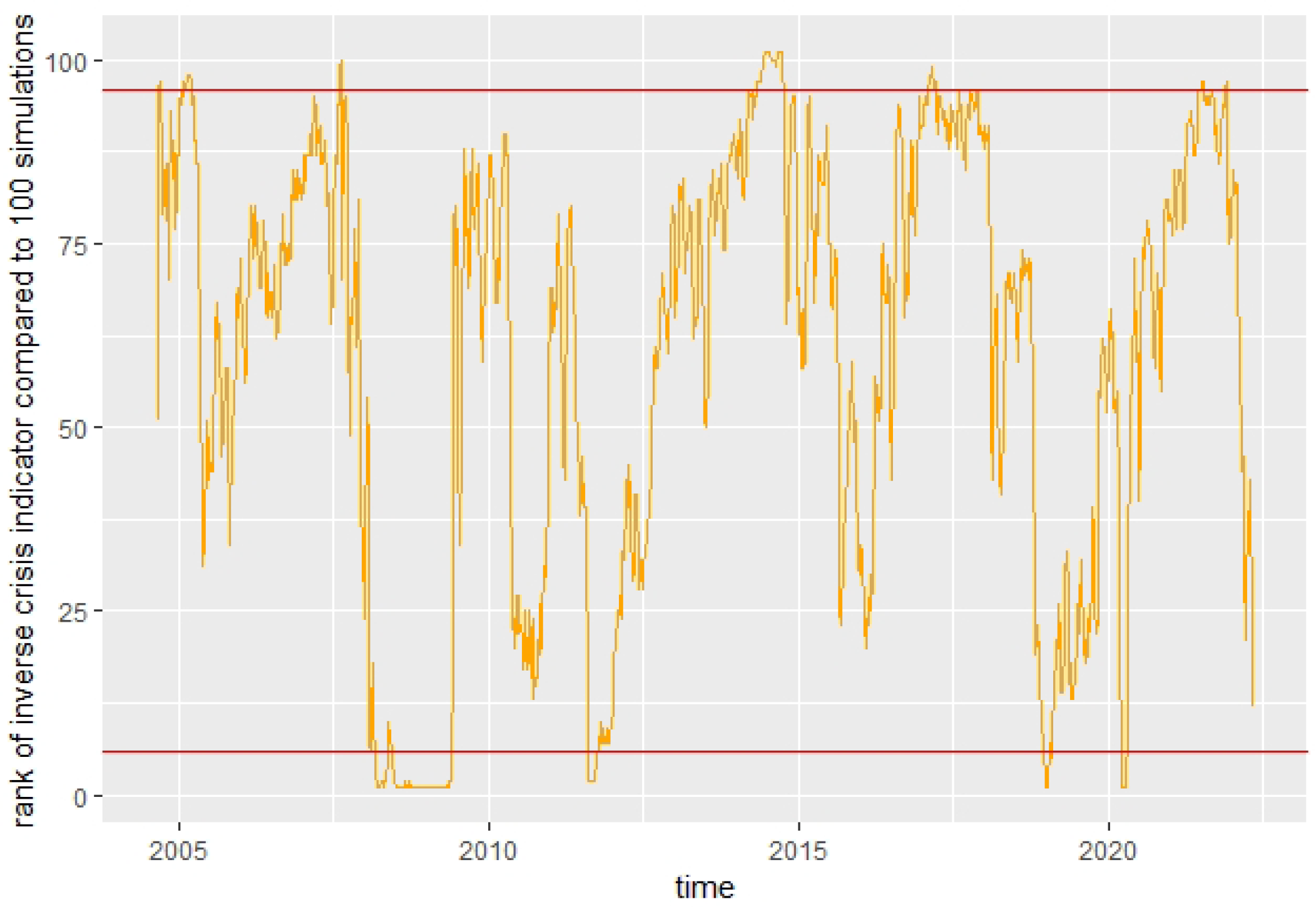
We also use the 100 simulated paths for the market indicator to look at every time point at the rank of the observed market indicator compared to the 100 simulations. A rank of 1 means that all 100 simulated values are greater than the observed value and a rank of 101 indicates that all 100 observations are smaller than the observed value. In Figure 4, we can see that the rank never stays at one of the extremes. Additionally, the ranks represent the quantiles of the distribution of the simulated market indicator, so if the observed market indicator is fitted well by our model, we expect, at 90% of the time points, the rank to be in the 90% middle part of the ranks, and thus between 6 and 96, indicated by the red lines in Figure 4. This is the case at 87.3% of the time points, which is very close to the expected 90%, indicating a reasonable fit for the model. The slightly lower value is probably caused by the extreme financial crisis in 2008, which generated extremely low values for the market indicator for a long time, thus generating, for unusually many time points (8.6%), ranks below 6 instead of the expected 5%.

4.2. Fitting the Model for the Risky Asset

4.2.1. Parameter Estimation

Next, we estimate the parameters of the model for the risky asset given in Definition 3 looking at the two special cases (10) and (11), using a maximum-likelihood estimation for the SDE of the logarithm of the discounted risky asset R 1 ( t ) = log P 1 ( t ) P 0 ( t ) given by
d R 1 ( t ) = μ ( C + X ( t ) ) Ψ X ( t ) 1 2 σ 2 ( C + X ( t ) ) Ψ X ( t ) 2 d t + σ C + X ( t ) Ψ X ( t ) d W P ( t ) .
As described above, we use the average US Treasury annualized 3-month rates for the time interval from 1 January 2005 to 2 May 2022 as constant interest rate r = 0.0119 .
For the case C = 0 in the model formulation in Definition 3, we use Ψ ( x ) = log ( 1 + x ) x such that we have the special case that we constructed in (11) following the theoretical considerations in Remark 3. With this, we can directly proceed with the log-likelihood maximization to obtain the estimates μ = 0.1202199 and σ = 0.2482996 . In this case, we assume that a correlation is possible, which we estimate additionally to be ρ = 0.0433 .
For the case ρ = 0 , we use Ψ ( x ) = ( C + x ) l such that we have the special case (10) that we established following the theoretical considerations from Remark 3. This means that the log-likelihood not only depends on the unknown parameters μ and σ but additionally on the unknown parameters C and l. Therefore, we perform the maximum-likelihood estimation for different combinations of the values for C and l and choose the resulting estimates μ and σ that achieve the best likelihood. This procedure leads to an increasingly better likelihood while C 0 . As C has to be strictly positive by assumption, we limit C from below by 0.05. As parameters and estimates, we obtain C = 0.05 , l = 0.8 , μ = 0.1017024 and σ = 0.1642218 . We estimate the correlation of W P and W X proceeding the same way as for the case C = 0 and obtain that ρ = 0.0288 , which is low enough for the assumption ρ = 0 appear reasonable.
All maximum-likelihood estimations were performed using a quasi-Newton BFGS method. No severe numerical instabilities were experienced in any of the estimations, and the obtained results appeared to be plausible.
In the following sections, we call our model the ‘Indicator model’ and the corresponding optimal strategy the ‘Indicator Strategy’. As a comparison model that does not take the crisis information into account, we choose a Black–Scholes (BS) model for the risky asset with drift r + μ ( B S ) and volatility σ ( B S ) , where we again use the average US 3m Treasury rates of 1 January 2005 to 2 May 2022 as constant r. We estimate its parameters to be μ ( B S ) = 0.079633 and σ ( B S ) = 0.178765 .

4.2.2. Goodness of Fit Comparison

We show that the formulation of our market model as specified in Definition 3 with the parameters estimated in Section 4.2.1 explains the market dynamics better than the BS model. For the discretized transformed SDEs of the risky assets in each model, we use, as for the inverse crisis Indicator before, the Shapiro–Wilk normality test. In all three cases, the hypothesis of normality is clearly rejected. While the BS model is rejected with a p-value p < 10 15 , the Indicator model is only rejected with a p-value of p 10 9 for the case C = 0 and p 3 · 10 7 for the case ρ = 0 , indicating that the assumption of normality is violated less in the Indicator model. In all three cases, the histograms look very similar to the theoretical normal distribution, except for a higher concentration of values around zero.
Further, we use the drift of the discretized SDE on the discounted log-prices ( Δ R 1 ( t i ) ) i = 1 , , n ( pred ) and compare these to the observed discounted log-returns ( Δ R 1 ( t i ) ) i = 1 , , n 1 . We perform this by calculating the root-mean-squared-error (RMSE) given by
R M S E = i = 1 n Δ R 1 ( i ) Δ R 1 ( i ) ( pred ) n .
When calculating the RMSE ratio of the Indicator model and the BS model as R M S E ( I n d i c a t o r ) R M S E ( B S ) , a ratio smaller than one indicates a smaller error and thus a better fit of the Indicator model, and a ratio bigger than one indicates a worse fit. If we perform the calculation with the same data used for the parameter estimation, i.e., in-sample, we obtain a ratio of 0.9983769 < 1 for the case C = 0 and 0.9989651 < 1 for ρ = 0 , which indicates that the Indicator model fits the log-returns of the discounted asset prices slightly better than the BS model, which is also confirmed by the Diebold–Mariano test using the R-function ‘dm.test’ from the ‘forecast’ package [32] (v8.17.0). The theory behind this test described in [33] is to compare the prediction errors of both models and to test based on this time series which model fits the data better and whether one of them is significantly better. Using as alternative hypothesis that the Indicator model is better than the BS model and the opposite as the null hypothesis, we obtain for the case C = 0 the test statistic 1.0827 < 0 with p-value 0.1397 and, for the case ρ = 0 , the test statistic 0.97636 < 0 with p-value 0.1646. This substantiates the claim that the Indicator model is slightly better than the BS strategy, but the difference is not enough to reject the null hypothesis.
If we now calculate the RMSE ratio for out-of-sample data, we obtain for the case C = 0 the value 0.9993901 < 1 and, for the case ρ = 0 , the value 0.9995626 < 1 , again indicating a slightly better fit of the Indicator model compared to the BS model. The Diebold–Mariano test confirms these observations for the out-of-sample data, returning for the case C = 0 the value 0.50078 < 0 with p-value 0.3084 and, for the case ρ = 0 , the value 0.44992 < 0 with p-value 0.3265.
We can use the same tools to check the volatility terms. For this, we use the volatility term of the log-returns of the risky asset. This way, we can predict the volatility in the BS model as
Vol 1 ( i ) pred = σ ( B S ) Δ t
and in the Indicator model as
Vol 1 ( i ) pred = σ C + X ( i ) Ψ ( X ( i ) ) Δ t .
As observable volatility of the log-returns, we use for every time point the standard deviation of the last 30 trading days up to the given day and denote the observed volatilities as Vol 1 ( i ) . Then, the RMSE is given as
R M S E = i = 1 n Vol 1 ( i ) Vol 1 ( i ) ( pred ) n .
We again first perform the RMSE calculations in-sample and obtain a ratio of 0.7658209 < 1 for the case C = 0 and 0.7147594 < 1 for ρ = 0 , indicating a much better fit to the observed volatilities of the asset log-returns for the Indicator model than for the BS model.
The Diebold–Mariano test confirms these observations, stating that the Indicator model is significantly better than the BS model, with a p-value p < 10 15 for both cases.
Carrying out the same procedure for the RMSE ratio on out-of-sample data, we obtain for the case C = 0 the value 0.7422229 < 1 and, for the case ρ = 0 , the value 0.5616701 < 1 , again indicating a much better fit of the Indicator model compared to the BS model. Note that, for the case ρ = 0 , the RMSE is almost only half the size of the BS RMSE. The Diebold–Mariano test confirms these observations, with a significant p-value p < 10 15 for the overall out-of-sample data.
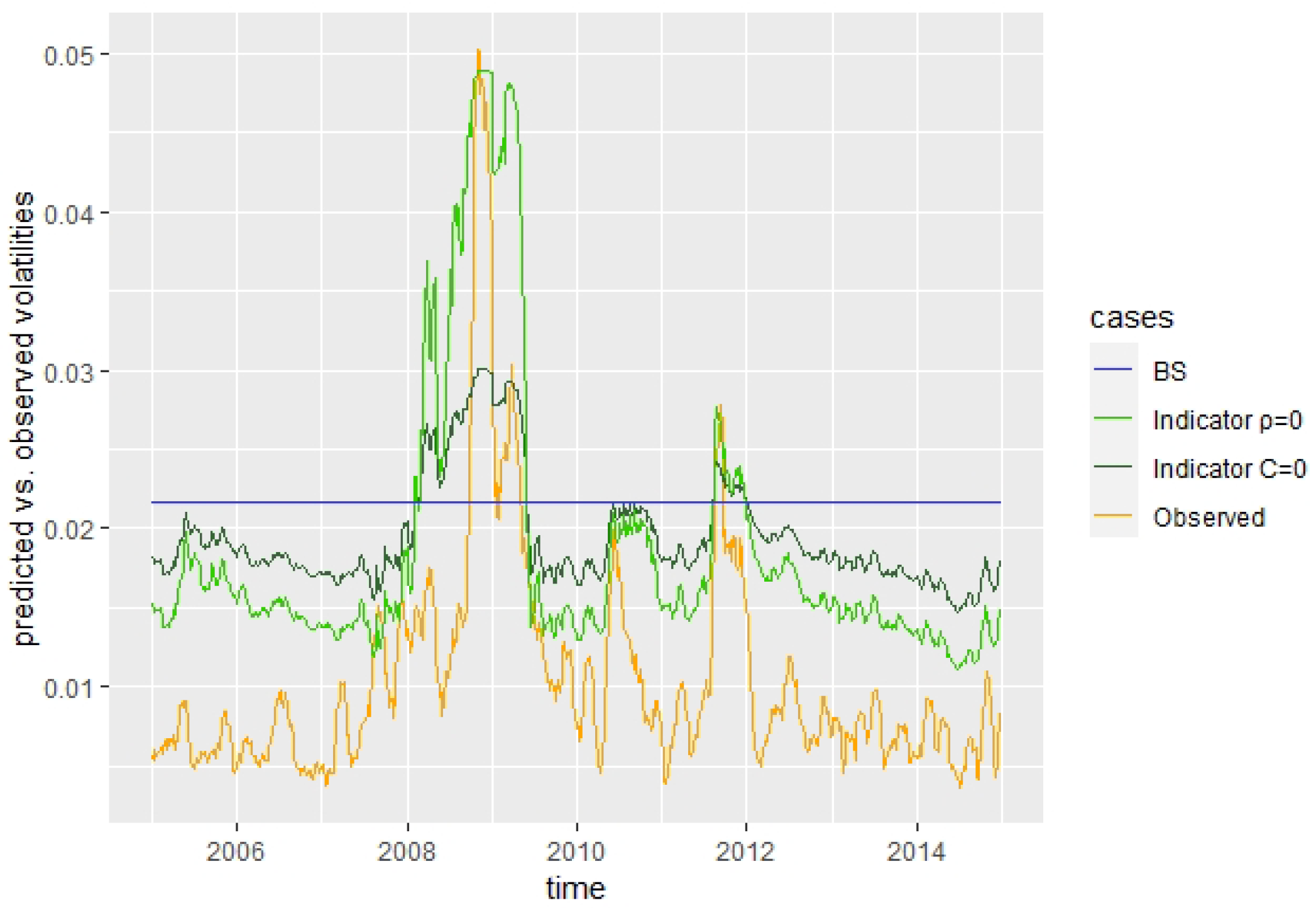
Figure 5 illustrates the better fit of the Indicator model to the observed volatilities compared to the BS model, which predicts a constant volatility.
As another test for the quality of our model, we use the SDEs of the risky asset for the case ρ = 0 , C = 0 and the BS model to simulate 100 paths of the risky asset for the whole time interval using the observed market indicator. With these paths, we derive monthly returns by calculating the return after five time steps of size Δ t .
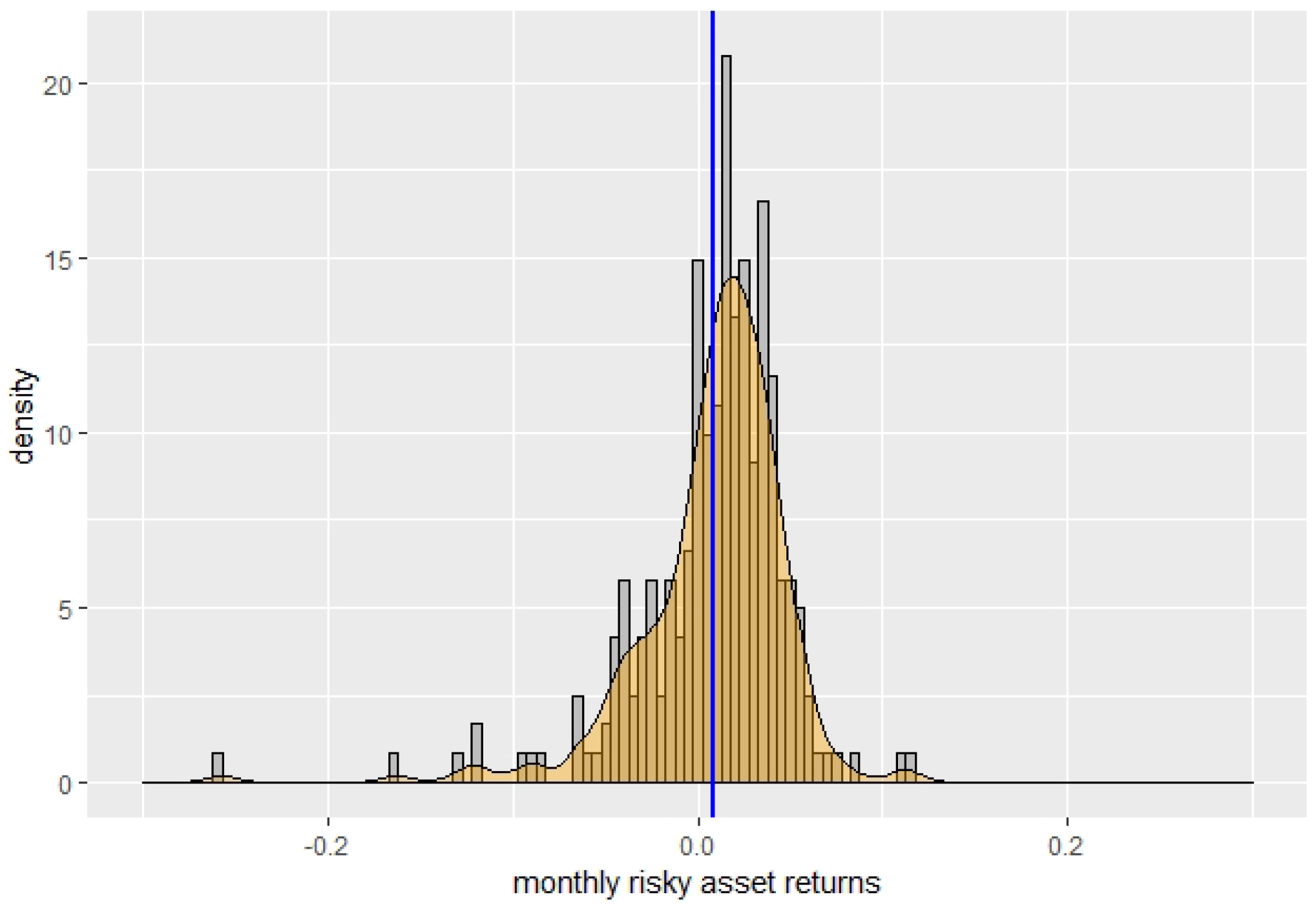
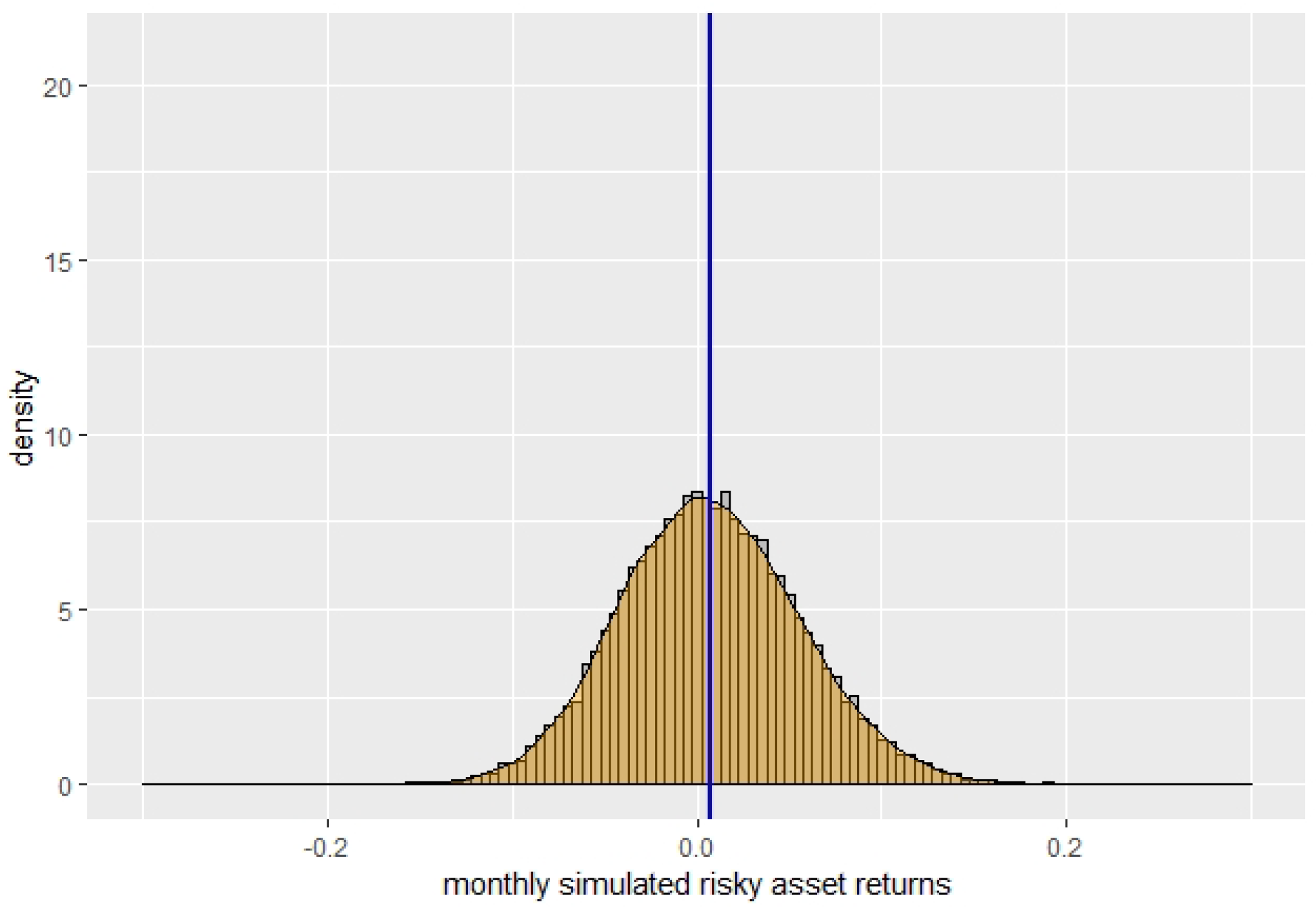
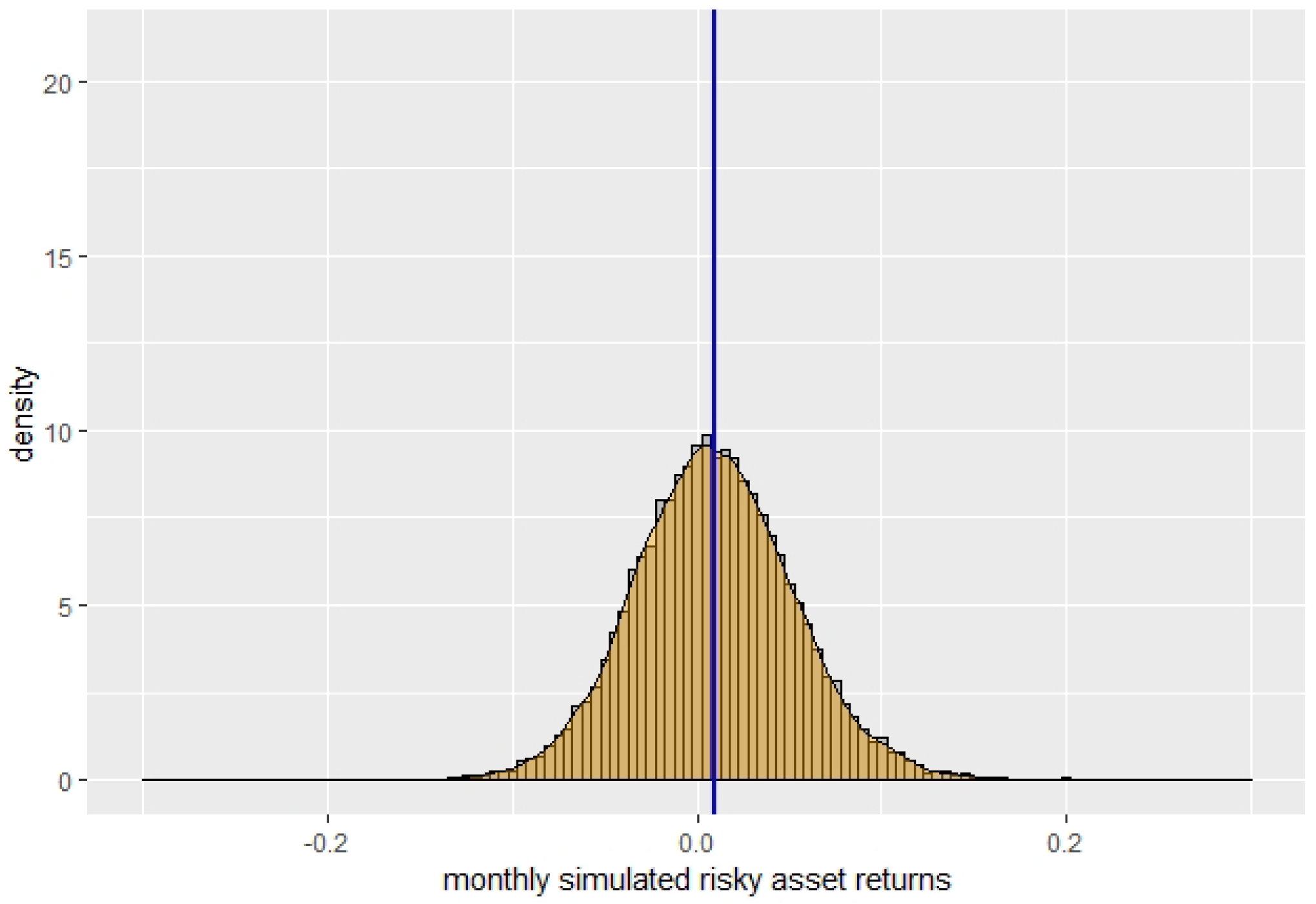
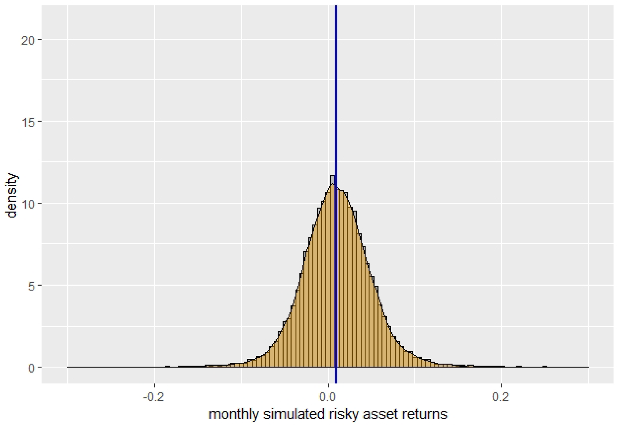
First, we perform in the same way as for the market indicator a χ 2 goodness of fit test, counting the frequencies of observed return data in intervals with size 0.02 between −0.07 and 0.07, and comparing it to frequencies for the same intervals obtained for the simulated data for each model. We obtain that the null hypothesis of a good fit is rejected for all three models. Still, while it is rejected most clearly for the BS model, with a p-value of p 9 · 10 14 , it is rejected for the Indicator models only with a higher p-value of p 10 7 for C = 0 and p 2 · 10 4 for ρ = 0 , indicating a better fit of the Indicator models compared to the BS model. In Figure 6, Figure 7, Figure 8 and Figure 9, we show the scaled histograms of the returns with the corresponding means indicated by the blue vertical line, overlaid by the kernel-smoothed empirical densities for the risky asset itself and the simulated risky asset for the three cases of the BS model, C = 0 and ρ = 0 . The distributions of the simulated returns exhibit less probability mass near the mean and in the tails than the observed returns, especially for the BS model, but are otherwise quite similar. Comparing the mean and standard deviation of the simulated monthly returns for those three cases to the mean and standard deviation of the monthly returns of the risky asset, we have the deviations for C = 0 (mean: 0.001115, s.d.: 0.002356), for the case ρ = 0 (mean: 0.001993, s.d.: 0.001513) and for the BS model (mean: −0.000832, s.d.: 0.008063). The absolute difference in the mean is slightly lower for the BS case compared to the others, but the absolute difference in the standard deviation is clearly highest for the BS case.
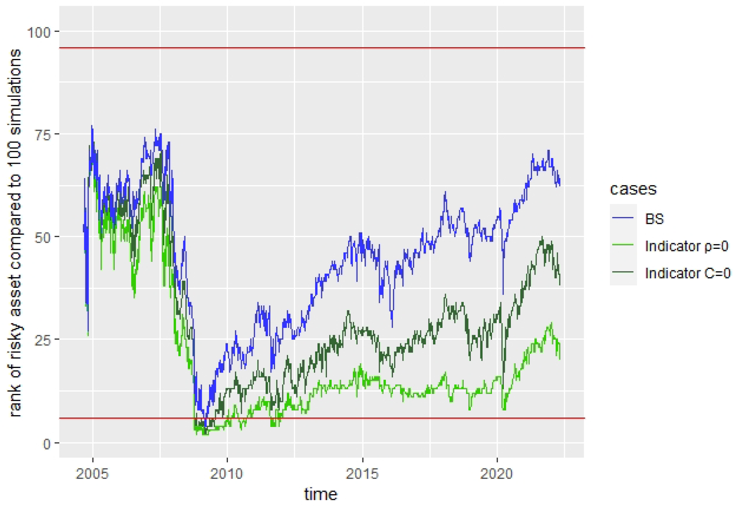
As for the market indicator, we also use the simulated paths for each case to observe whether the simulation looks reasonable. For this, we look again at every time point at the rank of the observed risky asset compared to the 100 simulations of a given case. The evolution of this rank statistic is shown in Figure 10. The ranks do not tend to occupy the extremes near 1 or 101. We would again expect to have at 90% of the time points a rank between 6 and 96, which is the middle 90% of the 100 possible ranks. We have that the middle 90% rank values are occupied for the BS model at 99.8% and, for the Indicator models, 98.4% and 97.8% of the time points for C = 0 and ρ = 0 , respectively. While all percentages are a bit too high, the Indicator models are nearest to the expected percentage.
Additionally, we perform these tests simulating paths without using the observed market indicator values, i.e., we simulate paths of the market indicator. When generating random independent normal values for the simulation, we generate for the case C = 0 the correlation between any normal random variable for the market indicator N X and a corresponding normal random variable for the risky asset N P by using instead the mixed normal random variable N = ρ N X + 1 ρ 2 N P . With the resulting simulated paths, we perform in the same way as before a χ 2 goodness of fit test, counting the frequencies of observed return data in intervals with size 0.02 between −0.07 and 0.07 and comparing them to frequencies for the same intervals obtained for the simulated data for each model. Again, the null hypothesis of a good fit is rejected for all three models. Once more, we can observe that, while it is rejected most clearly for the BS model, with a p-value of p 9 · 10 14 , it is rejected for the Indicator models only with a higher p-value of p 4 · 10 8 for C = 0 and p 5 · 10 5 for ρ = 0 , indicating again a better fit of the Indicator models compared to the BS model. The scaled histograms of the returns overlaid by the kernel-smoothed empirical densities of the risky asset itself and the simulated risky assets for the three cases of the BS model, C = 0 and ρ = 0 based on the simulated inverse crisis indicator show the same as before. Comparing the mean and standard deviation of the simulated monthly returns for those three cases to the mean and standard deviation of the monthly returns of the risky asset, we have the deviations for C = 0 (mean: 0.000816, s.d.: 0.00246), for the case ρ = 0 (mean: 0.001768, s.d.: −0.001713) and for the BS model (mean: −0.000832, s.d.: 0.008063). The absolute difference in the mean is lowest for the case C = 0 , followed by the BS case, but the absolute difference in the standard deviation is clearly highest for the BS case.
As before, we also look at every time point at the rank of the observed risky asset compared to the 100 simulations of a given case. The development of this rank statistic is shown in Figure 11 and looks very similar to the cases using the observed inverse crisis indicator. The ranks again do not tend to occupy the extremes near 1 or 101. The middle 90% rank values between 6 and 96 are occupied for the BS model at 99.8% and, for the Indicator models, at 96.1% and 90% of the time points for C = 0 and ρ = 0 , respectively. While the percentage for the BS model stayed equal because the simulation did not depend on the inverse crisis indicator, the other percentages were reduced such that they are even closer to the expected 90%, and the Indicator models are again nearest to the expected percentage.
Overall, we conclude that we have a good fit of the Indicator model for both cases of C = 0 and ρ = 0 , which are superior to the BS model, especially when comparing the fit of the volatility.

4.3. Strategy Performance Analysis

In this section, we compare the performance of our strategy derived in Theorem 1 (referred to as the ‘Indicator strategy’, with ‘Indicator C = 0 ’ denoting the case C = 0 and ‘Indicator ρ = 0 ’ denoting the case ρ = 0 ) to a case in the BS model, which does not consider the crisis information. The corresponding well-known optimal investment strategy in the BS model with HARA utility is given by
π ( B S ) = μ ( B S ) Φ V V σ ( B S ) 2 Φ V V = H μ ( B S ) V σ ( B S ) 2 = V F e r ( T t ) V μ ( B S ) σ ( B S ) 2 · 1 1 δ .
Remark 5. 
Looking back at the analysis of the Indicator strategy in Remark 4, we see that the structure for the BS strategy is very similar, with the difference being that we have a CPPI strategy with a constant instead of a stochastic multiplier. Hence, due to the absence of a stochastic factor, the hedging part disappears and the mean–variance part becomes constant.
Here, we compare the performance of the Indicator strategy in the out-of-sample time interval from 1 January 2015 to 2 May 2022 for the cases C = 0 and ρ = 0 to the BS strategy. We use the empirical crisis forecast data again to compare the performance of the strategies.
The starting point of the comparison horizon, denoted as t = 0 , is thus 1 January 2015, and the end point, denoted as t = T , is 2 May 2022. At t = 0 , we assume to start in all cases with a portfolio value of V ( 0 ) = 100 .
For the parameters of the HARA utility function introduced in Definition 4, we choose α = ( 1 δ ) δ 1 , as we then have for F = 0 the special case of the power utility. For the parameter δ , which influences the risk aversion, where lower values indicate a higher risk aversion, we compare the results for the values δ = 5 and δ = 10 (see [20]). The last parameter is the floor F. Note that the floor F is the guaranteed value of the portfolio at t = T , as it can be shown that the cushion given in (30) by C ( t ) = V ( t ) F e r ( T t ) is positive, implying that V ( t ) > F e r ( T t ) and thus guaranteeing at t = T a minimal value V ( T ) > F . Keeping this in mind, we also inspect the effect of different floors on the portfolio performance, where we have to make sure that F < V ( 0 ) e r ( T t ) in order to begin with a positive cushion C ( 0 ) . For the analysis, we choose F = 0 to obtain the power utility case without a guaranteed floor, as well as the floor levels F = 60 , which guarantee 60 % of the initial investment. In the simulation, the value V(t) was ensured to never fall below V ( t ) > F e r ( T t ) , where it would fall into a cash-lock scenario with π ( t ) = 0 for the remaining time. With the chosen small discrete time steps, this case did not occur in the simulation.
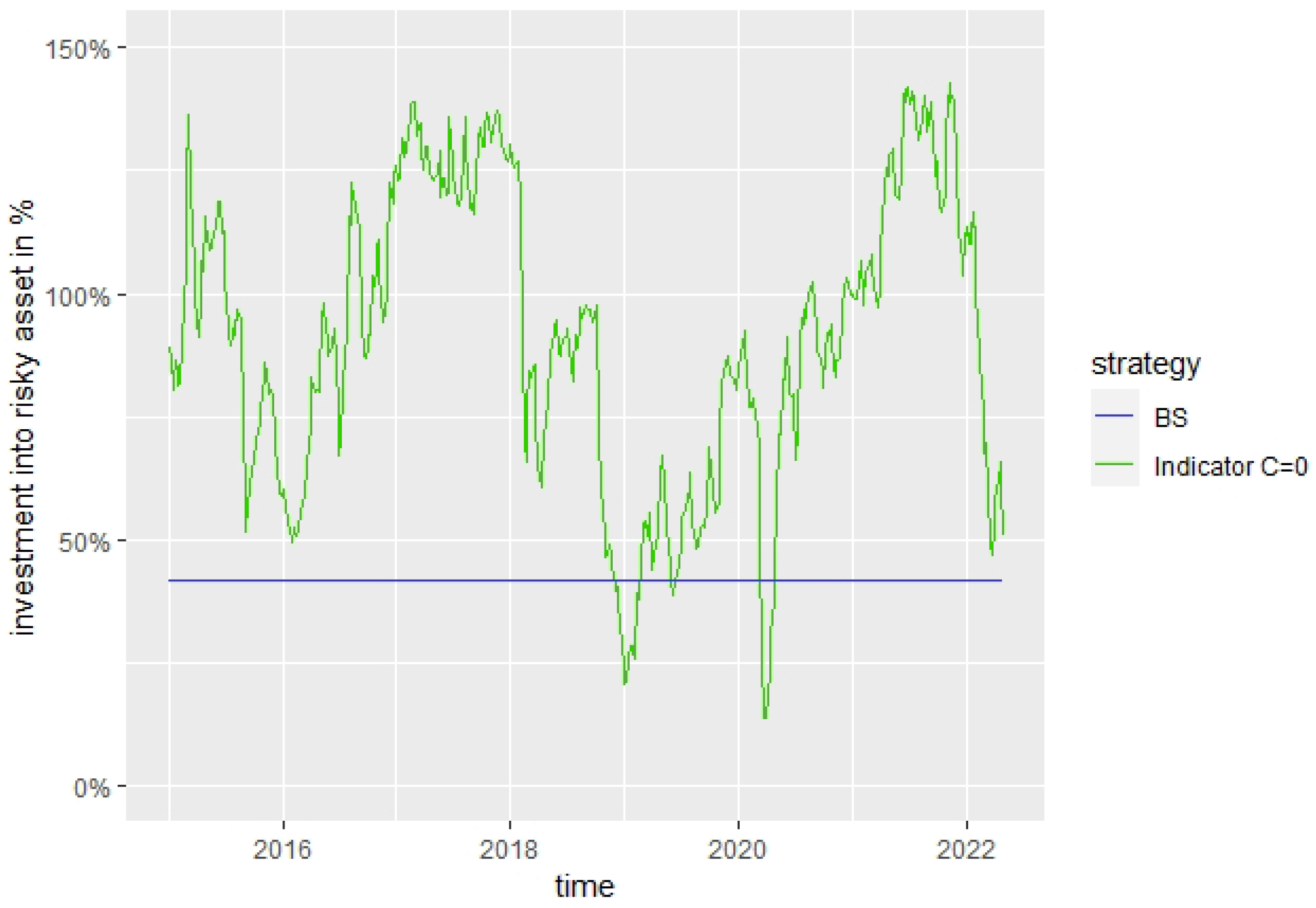
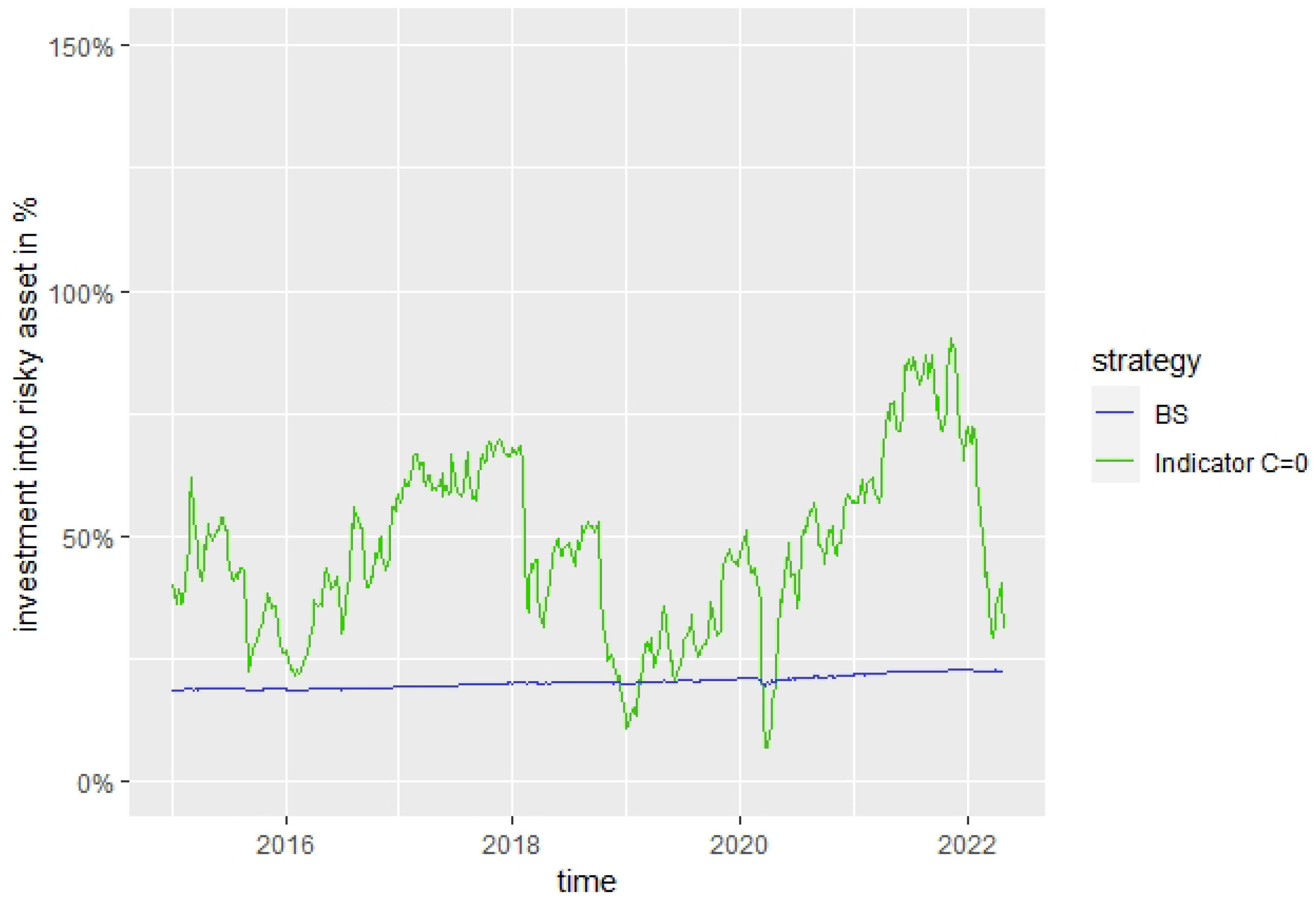
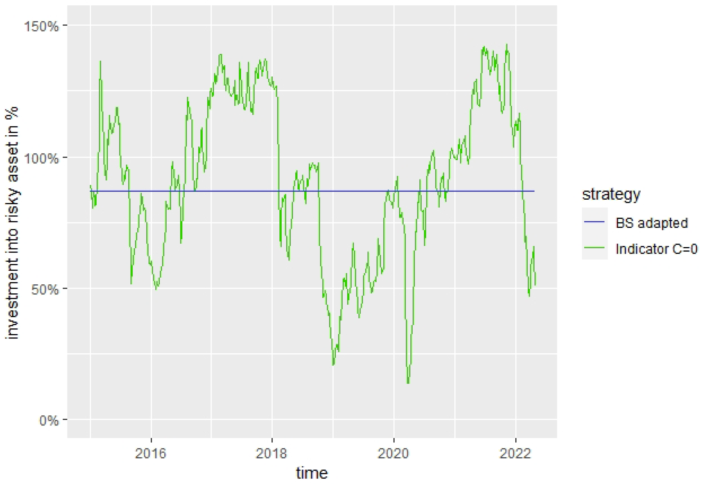
The development of the investment π (fraction of wealth) into the risky asset for the Indicator strategy with C = 0 and the BS strategy are shown in Figure 12 and Figure 13.
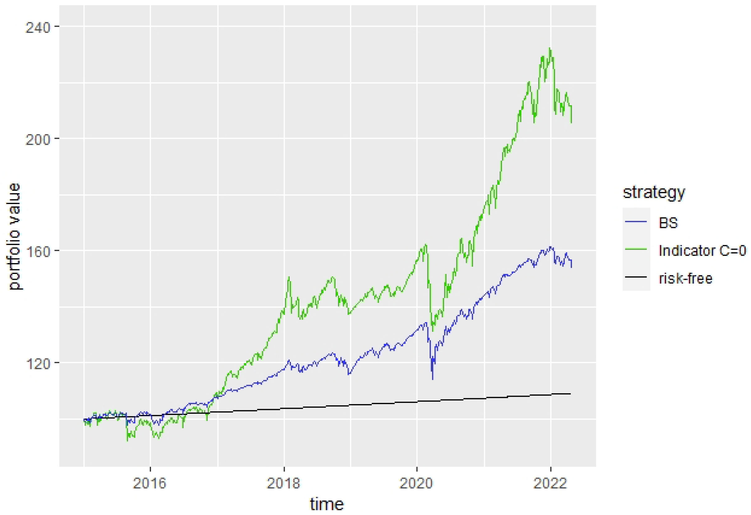
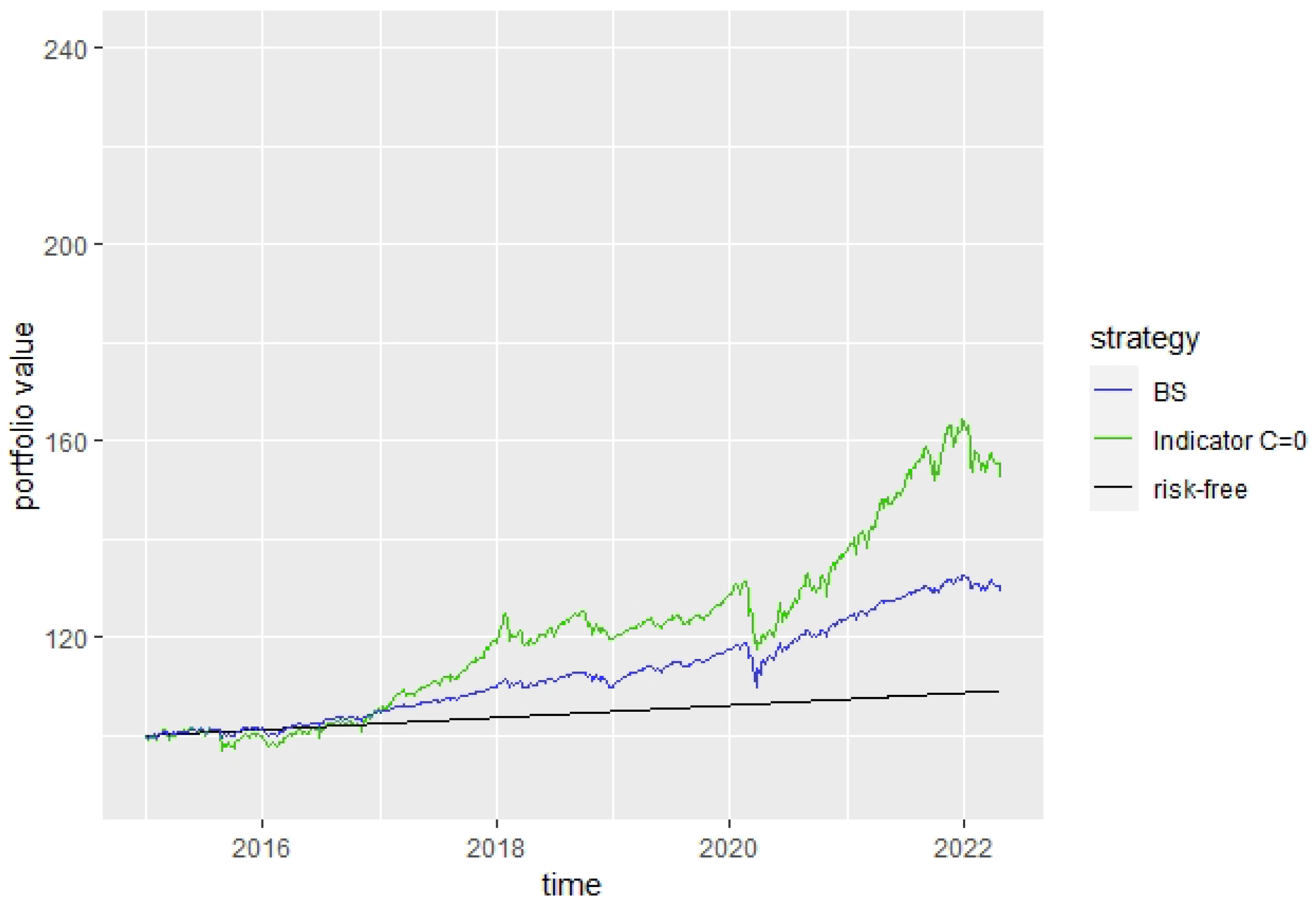
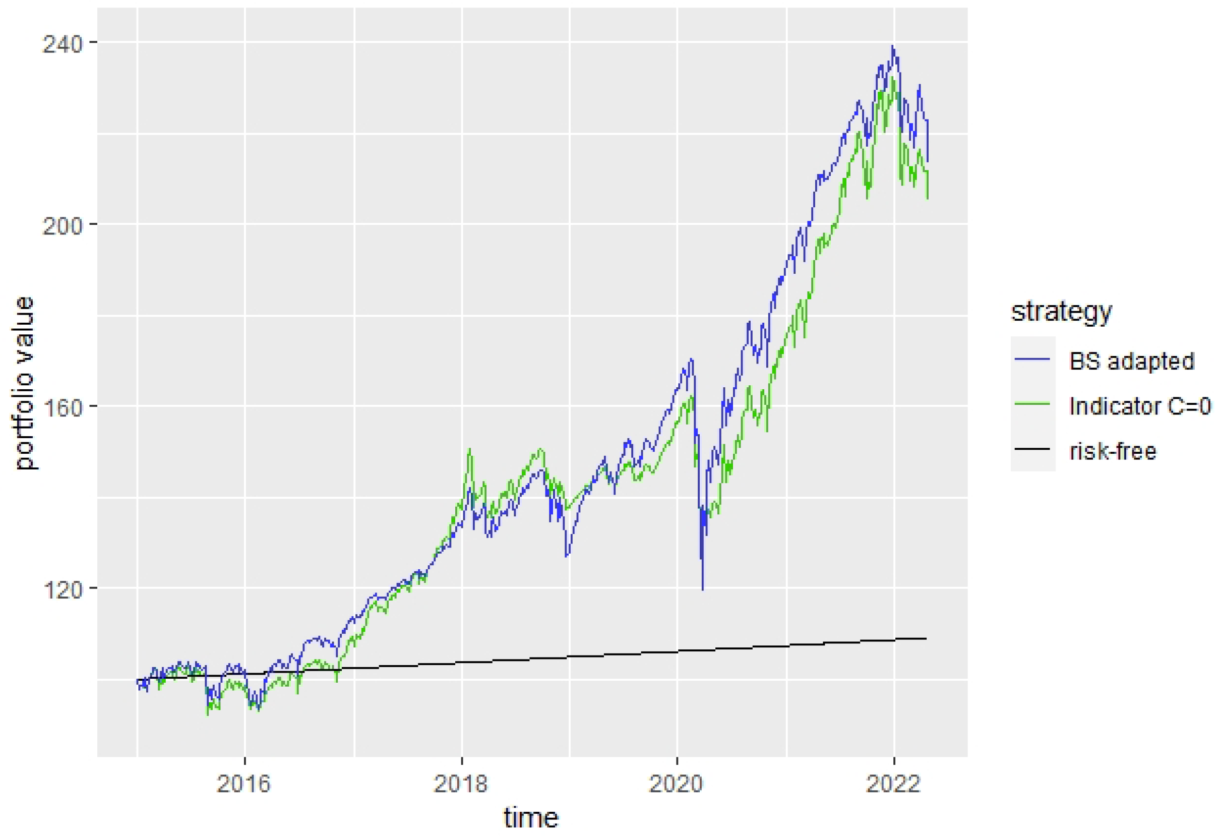
The corresponding portfolio value development for both strategies are shown in Figure 14 and Figure 15.
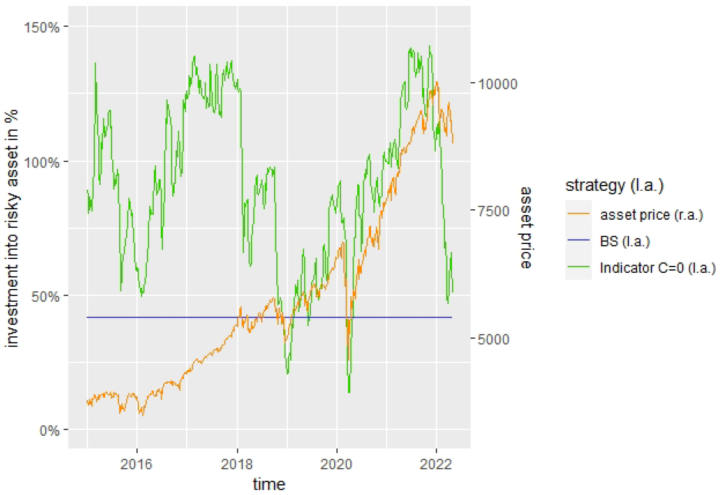
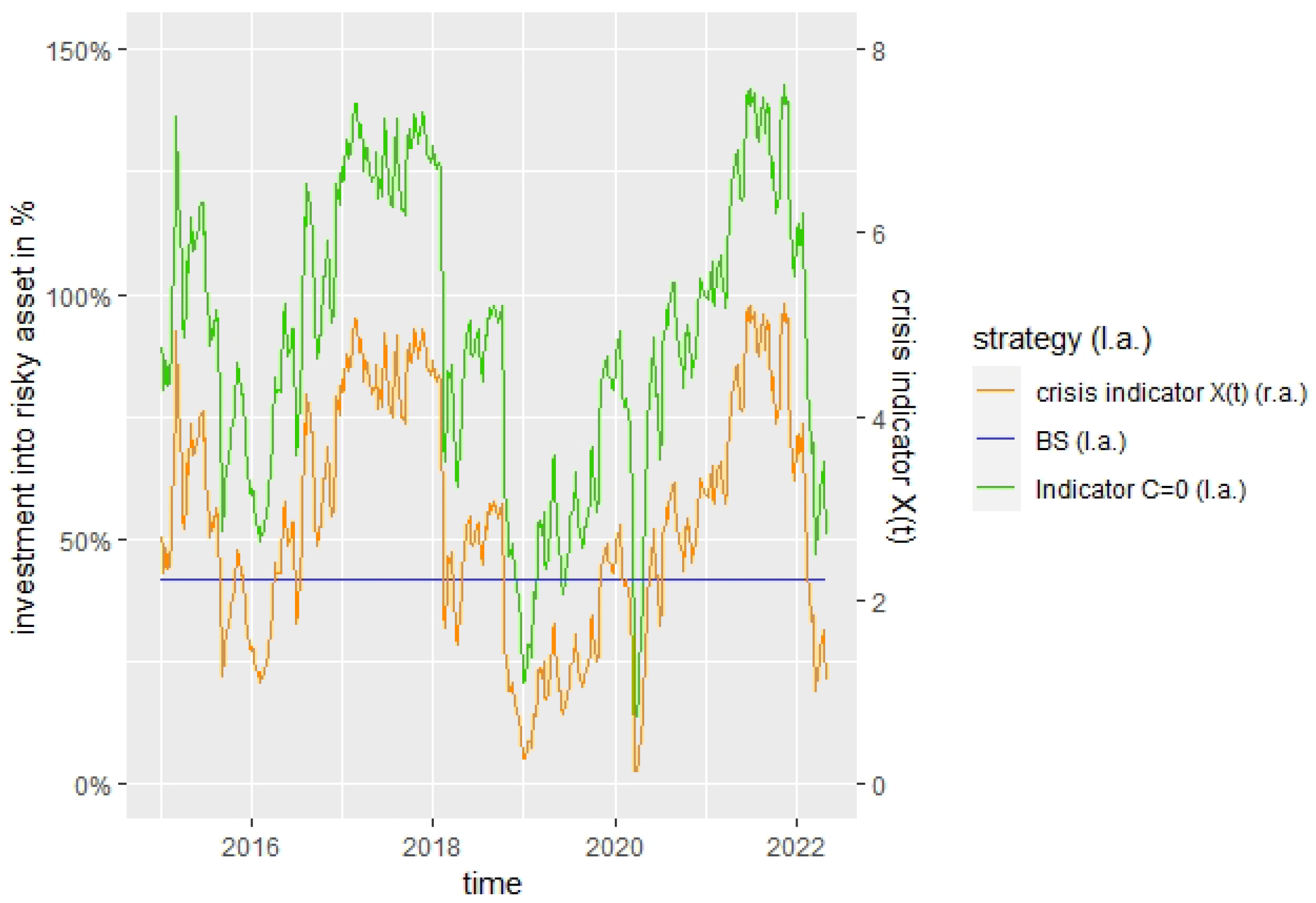
Note that the Indicator strategy constantly adapts the proportion invested into the risky asset according to the market indicator, as can be seen in Figure 16, where we set as an example F = 0 and δ = 5 . For instance, for the COVID-19 crisis in spring 2020, we can recognize that the strategy strongly decreased shortly after the asset prices started to decline, reaching a level below the BS investment into the risky asset. The small difference between the beginning of the asset price decline and the reaction of the inverse crisis indicator can explain the stronger decline in the portfolio value of the Indicator strategy compared to the BS strategy in Figure 14 and Figure 15, as the investment rate for the Indicator strategy was more than twice as high than for the BS strategy before. In Figure 17, it can be seen for the power utility how, for the Indicator strategy with C = 0 , the investment rate reacts to changes in the crisis indicator X ( t ) , which influences the stochastic multiplier described in Remark 4, in contrast to the constant investment rate and multiplier of the BS-strategy.
At the same time, the proportion invested into the risky asset by the BS strategy stays almost constant. The reason is that the optimal BS strategy does not depend on the market indicator and that the only factor leading to changes in the investment is the proportion from its cushion C ( t ) = V F e r ( T t ) to its portfolio value V ( t ) . For the power utility with floor F = 0 , the cushion is equal to the portfolio value, resulting in a constant investment of μ ( B S ) σ ( B S ) 2 · 1 1 δ of the BS strategy, as can be recognized in (43). For F > 0 , the strategy invests more into the risky asset when the cushion is big compared to the portfolio value, implying that it invests mostly less after a crisis when more of the cushion was consumed by the losses.
In general, it is clearly visible that the proportion invested into the risky asset decreases with higher risk aversion (lower δ ) and decreases with a higher guaranteed floor F as, in these cases, the strategies have to become more conservative to adapt to the higher risk aversion or to guarantee a higher final wealth level. These results are perfectly in line with our theoretical considerations concerning the optimal solution in Remark 4.
In Figure 18, it can be seen for the Indicator strategy with C = 0 that the mean–variance part of the stochastic multiplier described in Remark 4 has, in general, a higher influence than the hedging part. When the crisis indicator becomes small, indicating a high crisis probability, both parts decrease strongly to reduce the investment rate.
The most interesting observation is that the Indicator strategy almost always invests more into the risky asset than the BS strategy, except for strong crisis situations. This on-average significantly higher investment into the risky asset also helps the Indicator strategy to clearly outperform the BS strategy during this overall positive market phase, which is the case for every choice of parameter, as can be seen, e.g., in Figure 14 and Figure 15.
A reason for the low investment into the risky asset for the BS strategy seems to be that the BS parameters are estimated without considering the differences between crisis and non-crisis phases. To check this effect, we re-estimated the parameters of the BS model only considering phases with an estimated crisis probability ( p ( t ) ) t 0 below 90%, meaning that we only eliminated data points with a very high forecasted crisis probability of above 90%. To emphasize how seldom these levels occur, we need to consider that, during the 7-year out-of-sample period, the forecasted probabilities of crisis never exceeded 75%. Still, in the data we used, the parameter estimation levels were higher than 90 % with very low returns and high volatility, which occurred during the global financial crisis 2008 and probably strongly influenced the BS parameter estimation. Using now the adapted BS parameters, the investment rate into the risky asset increases significantly such that the investment into the risky asset of the BS strategy is near to the mean investment of the Indicator strategy into the risky asset, as can be seen in Figure 19. Consequently, the portfolio performance is now more similar to the performance of the Indicator strategy, as can be seen in Figure 20. Despite this additional information for the adapted BS strategy and the resulting more favorable estimates, the Indicator strategy performs very similarly to the BS strategy due to the influence of the market indicator. Furthermore, we can recognize in Figure 20, e.g., for the COVID-19 crisis in spring 2020, that the losses during asset crashes are often a lot lower for the Indicator strategy than for the BS strategy.
Therefore, the significantly higher performance of the Indicator strategy compared to the BS strategy seems to be justified by the knowledge gained through the market indicator, indicating that including the market indicator can substantially increase the investment performance over a BS-based strategy.
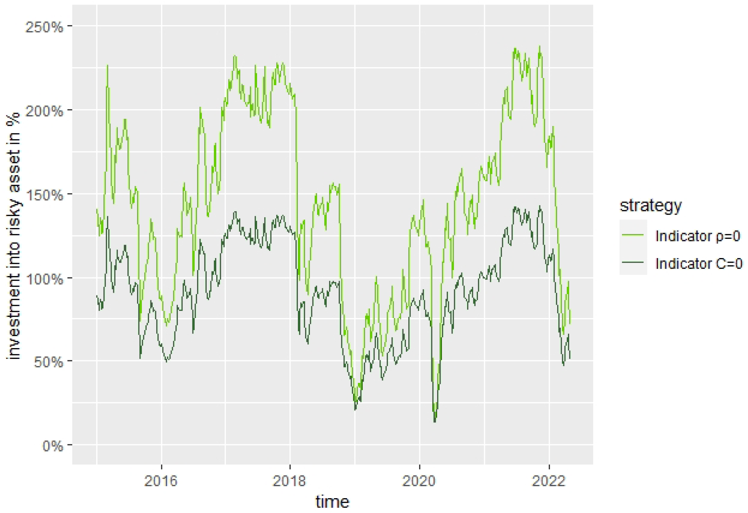
The analysis for the case ρ = 0 is very similar. The difference is that the Indicator strategy invests even more into the risky asset for the case ρ = 0 and hence outperforms the BS strategy even more than for the case C = 0 as can be seen in Figure 21. There, we can observe that the strategy ‘Indicator ρ = 0 ’ reduces its investment into the risky asset in times of crisis approximately to the same level as the strategy ‘Indicator C = 0 ’, but increases its investment in calm times much more than the strategy ‘Indicator C = 0 ’.
Finally, we compare different risk parameters, with the results in the different cases given in Table 1, where the best values in the comparison of Indicator strategies with C = 0 and ρ = 0 , as well as the BS strategy, are indicated in red.
We can see that both Indicator strategies have a better Sharpe Ratio and a better Adjusted Sharpe Ratio for any combination of parameters than the BS strategy. In addition, the values are rather stable for different risk-aversion parameters δ and decrease for an increasing floor F. Thus, the Indicator strategies seem to have a better ratio of excess return to volatility. To measure the size of the effect and test its significance, a Jobson & Korkie hypothesis test described in [34] with the correction by Memmel described in [35] was carried out. The normalized difference in Sharpe Ratios between the strategy ‘Indicator C = 0 ’ and the BS strategy is, at 2.27, clearly larger than 0, where the one-sided hypothesis test results compared to the asymptotic standard normal distribution under H 0 have a p-value of p = 0.012 . Using the Adjusted Sharpe Ratios, the normalized difference is 2.19, resulting in a p-value of p = 0.014 . For the strategy ‘Indicator ρ = 0 ’, we obtain, for the normalized difference in the Sharpe Ratios compared to the BS strategy, a value of 2.53, resulting in a p-value p = 0.006 . Using the Adjusted Sharpe Ratio, we also obtain a normalized difference of 2.26 and thus a p-value p = 0.012 . Hence, in all cases, H 0 can be rejected on a 1.5 % level.
Concerning the Omega, the values are very close to each other, where, depending on the parameters, different strategies achieve the highest value. In general, the Omega decreases for an increasing floor F. For different risk-aversion parameters δ , the Omega is rather stable.
The maximum drawdown decreases as expected with an increasing floor value F and increasing risk aversion (decreasing δ ) as the strategy becomes more conservative. The Indicator strategies always have a higher maximum drawdown value because their investment into the risky asset is, in general, more aggressive than the BS strategy. For the case ρ = 0 (Indicator ρ = 0 ), the maximum drawdown is noticeably higher than for the case C = 0 (Indicator C = 0 ), which mirrors the observed more aggressive investment into the risky asset. Even though the market indicator helps both Indicator strategies to reduce the investment during a crisis below the value obtained in the BS case, the strategies lose, due to their aggressive investment, more than the BS strategy at first, until the market indicator reacts and helps the strategy to adapt.

5. Conclusions

We establish a market model, which includes crisis forecasts as a stochastic factor. For a portfolio optimization problem with the expected utility of terminal wealth, we derive the HJB equation. Using an affine ansatz justified by the use of a CIR process for the stochastic factor ( X ( t ) ) t 0 and certain affine expressions implied by the model definition, we further transform the PDE into a Riccati ODE and a simple ODE, which are easily solvable for the HARA utility function. As a last step, the optimality of the solution is verified.
The resulting solution is a generalization of a CPPI strategy with a stochastic multiplier depending on the market indicator ( X ( t ) ) t 0 . We observe that the strategy reduces its investment into the risky asset in times with a higher risk of an upcoming crisis, where we have low returns and high volatility, while it increases its investment into the risky asset otherwise. This allows for riskier investment compared to a CPPI strategy with a constant multiplier in good times, mitigating the effect of a crash through a reduction in the investment into the risky asset in bad times.
We compare the obtained strategy to an optimal investment strategy in a BS market in out-of-sample backtesting with historic data. The Indicator strategy generally allows for a higher investment in the risky asset than the BS-based CPPI strategy and achieves clear outperformance. This is even more the case for the model formulation with ρ = 0 than for C = 0 . Taking a look at some risk measures, this behavior leads to a higher drawdown for the Indicator strategy and a similar Omega, but the Sharpe Ratio and the Adjusted Sharpe Ratio are significantly higher. Moreover, we observe that the higher drawdown was caused by a strong decline due to the aggressive investment behavior at the beginning of a crisis, but that the strategy quickly adapts to the crisis phase, strongly reducing the investment into the risky asset, and hence reducing the losses from that point on as desired. A goodness of fit analysis also confirms a better fit of the derived model compared to the BS model.

Author Contributions

Conceptualization, M.W. and R.Z.; methodology, V.G., M.W. and R.Z.; software, V.G.; writing—original draft preparation, V.G., M.W. and R.Z.; writing—review and editing, V.G., M.W. and R.Z.; supervision, M.W. and R.Z. All authors have read and agreed to the published version of the manuscript.

Funding

This research received no external funding.

Data Availability Statement

The original contributions presented in this study are included in the article. Further inquiries can be directed to the corresponding author.

Conflicts of Interest

The authors declare no conflicts of interest.

Appendix A. Solution of the Riccati ODE (Lemma A1)

Definition A1. 
Let ( Z ( t ) ) t 0 = ( Z 1 ( t ) , , Z d ( t ) ) t 0 be a continuous d-dimensional semimartingale that can be decomposed into
Z ( t ) = Z ( 0 ) + M ( t ) + A ( t ) ,
where Z ( 0 ) R d is F ( 0 ) -measurable, ( M ( t ) ) t 0 R d is a local martingale with M ( 0 ) = 0 and ( A ( t ) ) t 0 R d is a process with finite variation over a finite interval for each path with A ( 0 ) = 0 .
Defining the process ( C ( t ) ) t 0 R d , d by
C i , j ( t ) : = M i ( t ) , M j ( t ) ,
we have the characteristics of the continuous semimartingale ( Z ( t ) ) t 0 given by the pair ( A , C ) .
Definition A2. 
Let ( Z ( t ) ) t 0 be a continuous d-dimensional semimartingale with characteristics ( A , C ) . Additionally, let ( μ Z ( t ) ) t 0 R d be a predictable process such that
A ( t ) = 0 t μ Z ( s ) d s
and ( Γ Z ) t 0 R d , d be a non-negative process that is a symmetric matrix for each t 0 satisfying
C ( t ) = 0 t Γ Z ( s ) d s .
Then, we have the differential characteristics of the continuous semimartingale ( Z ( t ) ) t 0 given by ( μ Z , Γ Z ) .
With these definitions, we cite Theorem 2.34 in [36], which itself originates from Corollary 3.4 in [37].
Theorem A1. 
Let ( Z ( t ) ) t 0 = ( Z 1 ( t ) , , Z d ( t ) ) t 0 be a d-dimensional continuous semimartingale with differential characteristics ( μ Z , Γ Z ) that are affine, thus satisfying
μ Z ( t ) = μ 1 ( t ) μ d ( t ) = α 1 0 ( t ) α d 0 ( t ) + i = 1 d Z i α 1 i ( t ) α d i ( t ) Γ Z ( t ) = Γ 11 ( t ) Γ 1 d ( t ) Γ d 1 ( t ) Γ d d ( t ) = β 11 0 ( t ) β 1 d 0 ( t ) β d 1 0 ( t ) β d d 0 ( t ) + i = 1 d Z i β 11 i ( t ) β 1 d i ( t ) β d 1 i ( t ) β d d i ( t ) ,
with deterministic functions α k i , β k l i : [ 0 , ) R , i { 0 , , d } , k , l { 1 , , d } .
Assume that there is a number p N with p d such that, for all t [ 0 , T ] , the following conditions ( i ) ( i v ) are satisfied:
(i) 
α k i ( t ) 0 if 0 i p , 1 k p , k i ;
(ii) 
α k i ( t ) = 0 if p + 1 i d , 1 k p ;
(iii) 
β k l i ( t ) = 0 if 0 i p , 1 k , l p unless k = l = i ;
(iv) 
β k l i ( t ) = 0 if p + 1 i d , 1 k , l d .
Assuming that, additionally, all α k i , β k l i , i { 0 , , d } , k , l { 1 , , d } are continuous in t [ 0 , ) and for some 1 k d , we have
α k i ( t ) + 1 2 β k k i ( t ) = 0 0 i d ,
then it holds for this k that e Z k ( t ) is a martingale.
We next state a lemma that describes the conditions and solution to Riccati ODEs, as the proof of Theorem 1 requires one to derive and solve Riccati ODEs. The lemma can be shown similarly to the proof of Proposition 5.1 in [18].
Lemma A1. 
Consider the Riccati ODE
B ˜ t ( t ) + d 1 d 2 B ˜ ( t ) + 1 2 d 3 B ˜ 2 ( t ) = 0
with d 3 > 0 and terminal condition B ˜ ( T ) = 0 , satisfying
d 2 2 > 2 d 1 d 3
and
d 2 + d 2 2 2 d 1 d 3 > 0 .
Additionally, define
a : = d 2 2 2 d 1 d 3
and
c : = d 2 a d 2 + a .
Then, the solution to the Riccati ODE is given by
B ˜ ( t ) = ( d 2 a ) 1 e a ( T t ) d 3 1 c e a ( T t ) .
Proof of Theorem 1.
For the proof, we follow the arguments in Chapter 4 of [36].
We start heuristically arguing with Bellman’s principle that, for any time shift h > 0 , we have
Φ ( t , v , x , π ) = sup π Λ ( t , v ) E Φ t + h , V π ( t + h ) , X ( t + h ) | F t
where V π ( t ) = v and X ( t ) = x .
In the following, we will often write as short-hand notation Φ or Φ ( t ) instead of Φ ( t , v , x ) or Φ ( t , V π ( t ) , X ( t ) , π ( t ) ) to reduce the exposition to notation.
Applying now Itô’s formula to the right-hand side of (A13) with the derivatives of Φ with respect to t, V and X and second derivatives with respect to V V , V X and X X denoted by Φ t , Φ V , Φ X , Φ V V , Φ V X and Φ X X , we can replace inside the expectation
Φ ( t + h ) = Φ ( t ) + t t + h Φ t ( s ) d s + t t + h Φ V ( s ) μ V d s + t t + h Φ X ( s ) μ X d s + 1 2 t t + h Φ V V ( s ) σ V 2 d s + 1 2 t t + h Φ X X ( s ) σ X 2 d s + t t + h Φ V X ( s ) σ V ρ σ X d s + t t + h Φ V ( s ) σ V d W P ( s ) + t t + h Φ X ( s ) σ X d W X ( s ) .
Taking now on the right-hand side the limit h 0 and interchanging limit and expectation, as well as assuming the necessary square-integrability to cancel the last two terms when evaluating the expectation, we obtain the Hamilton–Jacobi–Bellman (HJB) equation
sup π Λ ( t , v ) ( Φ t + V r + π μ ( C + X ) Ψ ( X ) Φ V + 1 2 V 2 π 2 σ 2 ( C + X ) Ψ ( X ) 2 Φ V V + κ θ X Φ X + 1 2 σ ^ 2 X Φ X X + ρ V π σ C + X Ψ ( X ) σ ^ X Φ V X ) = 0
with the first-order condition
V μ ( C + X ) Ψ ( X ) Φ V + π V 2 σ 2 ( C + X ) Ψ ( X ) 2 Φ V V + ρ V σ C + X Ψ ( X ) σ ^ X Φ V X = 0
and optimal solution candidate
π = μ Φ V V σ 2 Ψ ( X ) Φ V V + ρ C + X σ ^ X Φ V X V σ ( C + X ) Ψ ( X ) Φ V V ,
which also fulfills the second-order condition
V 2 σ 2 ( C + X ) Ψ ( X ) 2 Φ V V < 0
as long as Φ ( t , v , x ) is a strictly concave function in v, which will be shown later.
Reinserting the optimal π into Equation (A15) and rearranging, we obtain the supremum-free PDE
Φ t + V r μ 2 ( C + X ) Φ V V σ 2 Φ V V ρ μ C + X σ ^ X Φ V X V σ Φ V V Φ V + 1 2 μ Φ V σ Φ V V + ρ C + X σ ^ X Φ V X ( C + X ) Φ V V 2 ( C + X ) Φ V V + κ θ X Φ X + 1 2 σ ^ 2 X Φ X X ρ μ σ ^ C + X X Φ V X Φ V σ Φ V V + ρ σ ^ 2 X Φ V X 2 Φ V V = 0 .
Now, taking the utility function as guidance, we choose as ansatz for the value function
Φ ( t , v , x ) = 1 δ δ α 1 1 δ v F e r ( T t ) δ f ( t , x ) = : 1 δ δ α H δ f .
Note that, as the cushion v F e r ( T t ) can be shown to be always positive, ( H ( t ) ) t 0 0 . Also, the terminal condition Φ ( T , v , x ) = 1 δ δ ( v F e r ( T t ) ) δ leads to f ( T , x ) = 1 .
Inserting this ansatz with the corresponding derivatives into Equation (A19) and simplifying, we obtain
f t + f r δ + μ 2 ( C + X ) δ 2 σ 2 ( 1 δ ) + f X ρ μ σ ^ C + X X δ σ ( 1 δ ) + κ θ X + f X X 1 2 σ ^ 2 X + f X 2 f 1 2 ρ 2 σ ^ 2 X δ 1 δ = 0 .
We cannot apply the Feynman–Kac theorem to (A21) due to the last mixed term, so we use the transformation h = f 1 γ with γ = 1 δ 1 δ + δ ρ 2 0 to obtain
h t + h r δ + μ 2 ( C + X ) δ 2 σ 2 ( 1 δ ) 1 δ + δ ρ 2 1 δ + h X ρ μ σ ^ C + X X δ σ ( 1 δ ) + κ θ X + h X X 1 2 σ ^ 2 X = 0
with the terminal condition f ( T , x ) = 1 implying also that h ( T , x ) = f ( T , x ) 1 γ = 1 ,
Applying to Equation (A22) the Feynman–Kac theorem, we have for h ( t , x ) the implicit solution
h ( t , x ) = E exp t T δ r + μ 2 C + X ˜ ( s ) 2 σ 2 ( 1 δ ) 1 δ + δ ρ 2 1 δ d s | X ˜ ( t ) = x = exp δ r + μ 2 C 2 σ 2 ( 1 δ ) 1 δ + δ ρ 2 1 δ ( T t ) E exp t T μ 2 δ 2 σ 2 ( 1 δ ) 1 δ + δ ρ 2 1 δ X ˜ ( s ) d s | X ˜ ( t ) = x ,
where X ˜ ( t ) follows the SDE
d X ˜ ( t ) = ρ μ σ ^ C + X ˜ X ˜ δ σ ( 1 δ ) + κ θ X ˜ d t + σ ^ X ˜ ( t ) d W X .
To use the affine term structure of the CIR model, ( X ˜ ( t ) ) t 0 needs to be a CIR process itself, so the first summand needs to be affine linear in X ˜ , which is the case if we choose C = 0 or ρ = 0 . In both cases, we can then deduce an exponential affine structure for h ( t , x ) from (A23) given by
h ( t , x ) = exp δ r + μ 2 C 2 σ 2 ( 1 δ ) 1 δ + δ ρ 2 1 δ ( T t ) exp A ˜ ( t ) + B ˜ ( t ) x > 0 ,
with the terminal condition h ( T , x ) = 1 leading to the terminal conditions A ˜ ( T ) = 0 and B ˜ ( T ) = 0 .
We treat the two cases C = 0 and ρ = 0 separately.
C=0:
Inserting C = 0 and the ansatz (A25) into the PDE (A22) and dividing through h ( t , x ) > 0 , we get, rearranging and leaving away the dependence on t in the notation,
A ˜ t + B ˜ t X + μ 2 X δ 2 σ 2 ( 1 δ ) 1 δ + δ ρ 2 1 δ + ρ μ σ ^ X δ σ ( 1 δ ) + κ θ X B ˜ + 1 2 σ ^ 2 X B ˜ 2 = 0 .
Note that this is a polynomial of degree 1 in X equating to zero; thus, the coefficients for X 0 and X 1 also have to be zero each, giving us the ODEs
A ˜ t + κ θ B ˜ = 0 , A ˜ ( T ) = 0 and
B ˜ t + μ 2 δ 2 σ 2 ( 1 δ ) 1 δ + δ ρ 2 1 δ + ρ μ σ ^ δ σ ( 1 δ ) κ B ˜ + 1 2 σ ^ 2 B ˜ 2 = 0 , B ˜ ( T ) = 0 .
The second ODE is a Riccati ODE, which only depends on ( B ˜ ( t ) ) t 0 . Using Lemma A1 with
d 1 = μ 2 δ 2 σ 2 ( 1 δ ) 1 δ + δ ρ 2 1 δ d 2 = κ ρ μ σ ^ δ σ ( 1 δ ) d 3 = σ ^ 2 > 0 .
It is easy to verify that the conditions of Lemma A1 are fulfilled due to the assumptions made in the theorem, and we obtain
B ˜ ( t ) = ( κ ρ μ σ ^ δ σ ( 1 δ ) a ¯ ) 1 e a ¯ ( T t ) σ ^ 2 1 c ¯ e a ¯ ( T t )
with a ¯ and c ¯ as stated in the theorem. Given this solution for ( B ˜ ( t ) ) t 0 , the solution for the first ODE in (A27) can be simply derived, together with the terminal condition A ˜ ( T ) = 0 through integration, to be
A ˜ ( t ) = t T κ θ B ˜ ( s ) d s = κ θ κ ρ μ σ ^ δ σ ( 1 δ ) a ¯ σ ^ 2 T t + ( 1 c ¯ ) ln 1 c ¯ 1 c ¯ e a ¯ ( T t ) c ¯ a ¯
and f ( t , X ( t ) ) as well as Φ t , V ( t ) , X ( t ) follow as given in the theorem. Inserting the derivatives of Φ t , V ( t ) , X ( t ) and f ( t , X ( t ) ) into (A17), we also obtain the solution π ( t , V ( t ) , X ( t ) ) given in the theorem.
ρ = 0 :
In this case, we have h ( t , x ) = f ( t , x ) as γ = 1 . Inserting ρ = 0 and the corresponding ansatz (A25) into (A21), we obtain, dividing by f ( t , x ) > 0 and rearranging terms,
A ˜ t + B ˜ t X + δ μ 2 X 2 σ 2 ( 1 δ ) + κ θ X B ˜ + 1 2 σ ^ 2 X B ˜ 2 = 0 .
This is again a polynomial in X of degree 1, so, as it equates to zero, the coefficients of X 0 and X 1 have to be zero each, leading to the ODEs
A ˜ t + κ θ B ˜ = 0 , A ˜ ( T ) = 0 and
B ˜ t + μ 2 δ 2 σ 2 ( 1 δ ) κ B ˜ + 1 2 σ ^ 2 B ˜ 2 = 0 , B ˜ ( T ) = 0 .
The second ODE is again a Riccati ODE, which only depends on ( B ˜ ( t ) ) t 0 . So, using Lemma A1, this time with
d 1 = μ 2 δ 2 σ 2 ( 1 δ ) d 2 = κ > 0 d 3 = σ ^ 2 > 0 ,
the conditions for Lemma A1 are again fulfilled due to the assumptions made in the theorem, and we obtain the solution
B ˜ ( t ) = ( κ a ˜ ) 1 e a ˜ ( T t ) σ ^ 2 1 c ˜ e a ˜ ( T t )
with a ˜ and c ˜ as stated in the theorem.
With this solution for ( B ˜ ( t ) ) t 0 , again through integration, the first ODE can be solved using the terminal condition A ˜ ( T ) = 0  to derive
A ˜ ( t ) = t T κ θ B ˜ ( s ) d s = κ θ κ a ˜ σ ^ 2 T t + ( 1 c ˜ ) ln 1 c ˜ 1 c ˜ e a ˜ ( T t ) c ˜ a ˜
and f ( t , X ( t ) ) as well as Φ t , V ( t ) , X ( t ) follow as given in the theorem. Inserting the derivatives of Φ t , V ( t ) , X ( t ) into (A17), we also obtain the solution π ( t , V ( t ) , X ( t ) ) given in the theorem.
Due to the heuristic derivations at the beginning, we still need to check that the cushion indeed stays positive as claimed during the proof and that the derived solution is actually optimal by showing that the value function for this strategy is equal to the maximum expected utility at every time point.
To do so for both cases in parallel, we denote the solutions for each case with a subscript ( i ) , where i { C , ρ } and i = ρ denotes the case with ρ [ 1 , 1 ] , and C = 0 and i = C denotes the case with C > 0 , ρ = 0 . With this in mind, we can write the candidate optimal solution as
π ( i ) ( t , V ( t ) , X ( t ) ) = V ( t ) F e r ( T t ) V ( t ) π ˜ ( i ) ( t , X ( t ) )
with
π ˜ ( ρ ) ( t , X ( t ) ) = 1 1 δ μ σ 2 Ψ ( X ( t ) ) + ρ 1 δ 1 δ + δ ρ 2 σ ^ σ Ψ ( X ( t ) ) B ˜ ( ρ ) ( t )
and
π ˜ ( C ) ( t , X ( t ) ) = 1 1 δ μ σ 2 Ψ ( X ( t ) ) .
Also, the respective value functions are then given by
Φ ( i ) ( t , V ( t ) , X ( t ) ) = 1 δ δ α 1 1 δ V ( t ) F e r ( T t ) δ exp w ( i ) ( T t ) + 1 δ 1 δ + δ ρ 2 A ˜ ( i ) ( t ) + B ˜ ( i ) ( t ) X ( t ) = 1 δ δ α 1 1 δ v F e r ( T t ) δ exp { w ( i ) T w ( i ) t + 1 δ 1 δ + δ ρ 2 ( A ˜ ( i ) ( 0 ) + 0 t A ˜ t ( i ) ( s ) d s + B ˜ ( i ) ( 0 ) x ( 0 ) + 0 t B ˜ t ( i ) ( s ) X ( s ) + B ˜ ( i ) ( s ) μ X ( x , s ) d s + 0 t B ˜ ( i ) ( s ) σ X ( x , s ) d W X ( s ) ) } ,
with
w ( C ) = δ r + μ 2 C 2 σ 2 ( 1 δ ) and w ( ρ ) = δ r ,
keeping in mind that μ X ( x , s ) and σ X ( x , s ) are known from the model formulation in Definition 3, as well as that the functions A ˜ ( C ) ( t ) , A ˜ t ( C ) ( t ) , A ˜ ( ρ ) ( t ) , A ˜ t ( ρ ) ( t ) , B ˜ ( C ) ( t ) , B ˜ t ( C ) ( t ) , B ˜ ( ρ ) ( t ) , B ˜ t ( ρ ) ( t ) are all continuous and were derived in the respective parts of the proof for C = 0 and ρ = 0 .
To ease the notation, we will continue to write Φ ( t , V ( t ) , X ( t ) ) and π ( t , V ( t ) , X ( t ) ) without the subscript when the distinction of the two cases is not relevant, and thus these variables represent both cases.
The positivity of the cushion ( C ( t ) ) t 0 = ( V ( t ) F e r ( T t ) ) t 0 can be shown with a similar idea to that in the proof of Theorem 6.5 in [36] by inserting the optimal solution candidate (A38) into the SDE of the cushion ( C ( t ) ) t 0 to derive the SDE of the cushion with solution
C ( t ) = C ( 0 ) exp { 0 t r + π ˜ ( i ) ( s , X ( s ) ) μ C + X ( s ) Ψ X ( s ) d s 0 t 1 2 π ˜ ( i ) 2 ( s , X ( s ) ) σ 2 ( C + X ( s ) ) Ψ 2 X ( s ) d s + 0 t π ˜ ( i ) ( s , X ( s ) ) σ C + X ( s ) Ψ X ( s ) d W P ( s ) } > 0 .
This expression for the cushion is positive as desired due to the positivity of the exponential function as long as C ( 0 ) > 0 , which is equivalent to the assumption that V ( 0 ) > F e r T .
Next, we show that the value function is, at every time point t [ 0 , T ] , an upper bound for the expected utility of any strategy. For this, we use the arguments given in the proof of Remark 4.5 in [36] (p. 162).
Using Itô’s formula and the supremum in the HJB equation, it is easy to see that
Φ ( T , V π ( T ) , X ( T ) ) Φ ( t , V π ( t ) , X ( t ) ) + t T Φ V ( s , V π ( s ) , X ( s ) ) σ V d W P ( s ) + t T Φ X ( s , V π ( s ) , X ( s ) ) σ X d W X ( s ) = : Y ( T ) .
Note that, by definition,
Y ( t ) = Φ ( t , V π ( t ) , X ( t ) )
and that ( Y ( t ) ) t 0 is a local martingale, as it has no drift. Taking advantage of the fact that Φ ( t , V ( t ) , X ( t ) ) 0 , we see that ( Y ( t ) ) t 0 is a non-negative local martingale and therefore it is a supermartingale. Thus, using (A44) in the first inequality and the supermartingale property of ( Y ( t ) ) t 0 in the second inequality, we obtain
E U ( V π ( T ) ) | F t = E 1 δ δ α 1 1 δ V π ( T ) F δ | F t = E Φ T , V π ( T ) , X ( T ) | F t E Y ( T ) | F t Y ( t ) = Φ t , V π ( t ) , X ( t ) ,
as desired.
To show that the value function is equal to the expected utility for our optimal strategy ( π ( t ) ) t 0 at every time point t [ 0 , T ] , we only need to show that the value function ( Φ ( t , V ( t ) , X ( t ) ) ) t 0 is a martingale for ( V π ( t ) ) t 0 . In that case, we directly get
E U ( V π ( T ) ) | F t = E 1 δ δ α 1 1 δ V π ( T ) F δ | F t = E Φ T , V π ( T ) , X ( T ) | F t = Φ t , V π ( t ) , X ( t ) .
To do so, we proceed as in the proof of Proposition 5.6 in [36] and define the process ( G ( t ) ) t 0 as
G ( i ) ( t ) = ln Φ ( i ) ( t , V π ( t ) , X ( t ) ) Φ ( i ) ( 0 , V π ( 0 ) , X ( 0 ) ) .
Inserting the value function from (A41) and then the solution for the cushion from (A43), we derive the SDE
d G ( i ) ( t ) = ( δ r w ( i ) + δ π ˜ ( i ) ( t , X ( t ) ) μ C + X ( t ) Ψ X ( t ) 1 2 δ π ˜ ( i ) 2 ( t , X ( t ) ) σ 2 ( C + X ( t ) ) Ψ 2 X ( t ) + 1 δ 1 δ + δ ρ 2 A ˜ t ( i ) ( t ) + B ˜ t ( i ) ( t ) X ( t ) + B ˜ ( i ) ( t ) μ X ( X ( t ) , t ) ) d t + δ π ˜ ( i ) ( t , X ( t ) ) σ C + X ( t ) Ψ X ( t ) d W P ( t ) + 1 δ 1 δ + δ ρ 2 B ˜ ( i ) ( t ) σ X ( X ( t ) , t ) d W X ( t ) = : μ ( i ) G d t + σ ( i ) G P d W P ( t ) + σ ( i ) G X d W X ( t ) .
Defining now the two-dimensional process ( Z ( i ) ( t ) ) t 0 with
Z ( i ) ( t ) = ( X ( t ) , G ( i ) ( t ) ) ,
we can easily see through the SDEs of ( X ( t ) ) t 0 in Definition 3 and ( G ( i ) ( t ) ) t 0 in (A49) that the differential semimartingale characteristics introduced in Definition A2 of ( Z ( i ) ( t ) ) t 0 are given by
μ 1 Z ( i ) = μ X μ 2 Z ( i ) = μ ( i ) G Γ 11 Z ( i ) = 1 d t σ X d W X , σ X d W X = σ X 2 Γ 12 Z ( i ) = Γ 21 Z ( i ) = 1 d t σ X d W X , σ ( i ) G P d W P + σ ( i ) G X d W X = 1 d t σ X d W X , σ ( i ) G X d W X + 1 d t σ X d W X , σ ( i ) G P d W P = σ X σ ( i ) G X + ρ σ X σ ( i ) G P = σ X σ ( i ) G X + ρ σ ( i ) G P Γ 22 Z ( i ) = 1 d t σ ( i ) G P d W P + σ ( i ) G X d W X , σ ( i ) G P d W P + σ ( i ) G X d W X = 1 d t σ ( i ) G X d W X , σ ( i ) G X d W X + 1 d t σ ( i ) G P d W P , σ ( i ) G P d W P + 2 1 d t σ ( i ) G X d W X , σ ( i ) G P d W P = σ ( i ) G X 2 + σ ( i ) G P 2 + 2 ρ σ ( i ) G X σ ( i ) G P .
Now, we see that, for the case ρ = 0 , all characteristics are affine such that we are in the framework of Theorem A1 with d = 2 , and we fulfill the conditions (i)–(iv) with
α 1 0 = κ θ α 2 0 = μ 2 C 2 σ 2 ( 1 δ ) + δ 1 δ μ 2 C σ 2 1 2 δ ( 1 δ ) 2 μ 2 C σ 2 + A ˜ t ( C ) + B ˜ ( C ) κ θ α 1 1 = κ α 2 1 = δ 1 δ μ 2 σ 2 1 2 δ ( 1 δ ) 2 μ 2 σ 2 + B ˜ t ( C ) B ˜ ( C ) κ α 1 2 = α 2 2 = 0 β 11 0 = β 12 0 = β 21 0 = 0 β 22 0 = δ 2 ( 1 δ ) 2 μ 2 C σ 2 β 11 1 = σ ^ 2 β 12 1 = β 21 1 = B ˜ ( C ) σ ^ 2 β 22 1 = B ˜ ( C ) 2 σ ^ 2 + δ 2 ( 1 δ ) 2 μ 2 σ 2 β 11 2 = β 12 2 = β 21 2 = β 22 2 = 0 ,
choosing p = 1 .
Also, for the case C = 0 , all characteristics are affine such that we are again in the framework of Theorem A1 with d = 2 , and these time conditions (i)–(iv) are fulfilled with
α 1 0 = κ θ α 2 0 = 1 δ 1 δ + δ ρ 2 A ˜ t ( ρ ) + B ˜ ( ρ ) κ θ α 1 1 = κ α 2 1 = δ 1 δ μ 2 σ 2 + ρ δ 1 δ + δ ρ 2 μ σ ^ σ B ˜ ( ρ ) + 1 δ 1 δ + δ ρ 2 B ˜ t ( ρ ) B ˜ ( ρ ) κ 1 2 δ ( 1 δ ) 2 μ 2 σ 2 + 2 ρ μ σ ^ σ 1 δ 1 δ + δ ρ 2 B ˜ ( ρ ) + ρ 2 σ ^ 2 1 δ 1 δ + δ ρ 2 2 B ˜ ( ρ ) 2 α 1 2 = α 2 2 = 0 β 11 0 = β 12 0 = β 21 0 = β 22 0 = 0 β 11 1 = σ ^ 2 β 12 1 = β 21 1 = 1 δ 1 δ + δ ρ 2 B ˜ ( ρ ) σ ^ 2 + ρ δ 1 δ μ σ ^ σ + ρ 2 δ 1 δ + δ ρ 2 σ ^ 2 B ˜ ( ρ ) β 22 1 = 1 δ 1 δ + δ ρ 2 B ˜ ( ρ ) σ ^ 2 + δ 1 δ μ σ + ρ δ 1 δ + δ ρ 2 σ ^ B ˜ ( ρ ) 2 + 2 ρ 1 δ 1 δ + δ ρ 2 B ˜ ( ρ ) σ ^ δ 1 δ μ σ + ρ δ 1 δ + δ ρ 2 σ ^ B ˜ ( ρ ) β 11 2 = β 12 2 = β 21 2 = β 22 2 = 0 ,
choosing again p = 1 .
Hence, in order to use, for both cases, Theorem A1, we just have to show that the condition (A6) therein is fulfilled. Using Itô’s formula on Φ ( i ) and noting that the HJB equation is attained at π ( i ) , we see that it has drift μ Φ ( i ) = 0 . At the same time, we have, due to (A48),
Φ ( i ) ( t ) = Φ ( i ) ( 0 ) exp { G ( i ) ( t ) } ,
which has, using Itô’s formula, the SDE for ( G i ( t ) ) t 0 from (A49) as well as, from (A51), the SDE
d Φ ( i ) ( t ) = Φ ( i ) ( t ) μ 2 Z ( i ) + 1 2 Γ 22 Z ( i ) d t + σ ( i ) G P d W P + σ ( i ) G X d W X .
Together, this leads to
0 = μ Φ ( i ) = Φ ( i ) ( t ) μ 2 Z ( i ) + 1 2 Γ 22 Z ( i ) = ( α 2 0 + 1 2 β 22 0 ) + ( α 2 1 + 1 2 β 22 1 ) X + ( α 2 2 + 1 2 β 22 2 ) G ( i ) .
We notice that the expressions in parentheses are zero as every coefficient of the polynomial in X and G ( i ) has to be zero. This is exactly the condition (A6) from Theorem A1, so we can apply in both cases Theorem A1 and obtain that e G ( i ) ( t ) is a martingale, which means that, plugging in the definition of ( G ( i ) ( t ) ) t 0 from (A48), we know that ( Φ ( i ) ( t ) ) t 0 is a martingale, which finalizes the proof. □

References

  1. Merton, R.C. Lifetime Portfolio Selection under Uncertainty: The Continuous-Time Case. Rev. Econ. Stat. 1969, 51, 247–257. [Google Scholar] [CrossRef]
  2. Hauptmann, J.; Hoppenkamps, A.; Min, A.; Ramsauer, F.; Zagst, R. Forecasting Market Turbulence Using Regime-Switching Models. Financ. Mark. Portf. Manag. 2014, 28, 139–164. [Google Scholar] [CrossRef]
  3. Dua, P.; Tuteja, D. Regime Shifts in the Behaviour of International Currency and Equity Markets: A Markov-Switching Analysis. J. Quant. Econ. 2021, 19, 309–336. [Google Scholar] [CrossRef]
  4. Bäuerle, N.; Rieder, U. Portfolio Optimization with Markov-Modulated Stock Prices and Interest Rates. IEEE Trans. Autom. Control 2004, 49, 442–447. [Google Scholar] [CrossRef]
  5. Sotomayor, L.R.; Cadenillas, A. Explicit Solutions of Consumption-Investment Problems in Financial Markets with Regime Switching. Math. Financ. 2009, 19, 251–279. [Google Scholar] [CrossRef]
  6. Nystrup, P.; Madsen, H.; Lindström, E. Dynamic Portfolio Optimization Across Hidden Market Regimes. Quant. Financ. 2018, 18, 83–95. [Google Scholar] [CrossRef]
  7. Capponi, A.; Figueroa-Lopez, J.E. Dynamic Portfolio Optimization with a Defaultable Security and Regime-Switching. Math. Financ. 2014, 24, 207–249. [Google Scholar] [CrossRef]
  8. Ernst, C.; Grossmann, M.; Höcht, S.; Minden, S.; Scherer, S.; Zagst, R. Portfolio Selection under Changing Market Conditions. Int. J. Financ. Serv. Manag. 2009, 4, 48–63. [Google Scholar] [CrossRef]
  9. Kritzman, M.; Page, M.; Turkington, D. Regime Shifts: Implications for Dynamic Strategies (corrected). Financ. Anal. J. 2018, 68, 22–39. [Google Scholar] [CrossRef]
  10. Ang, A.; Timmermann, A. Regime Changes and Financial Markets. Annu. Rev. Financ. Econ. 2012, 4, 313–337. [Google Scholar] [CrossRef]
  11. Chen, J.; Tsang, E.P.K. Classification of Normal and Abnormal Regimes in Financial Markets. Algorithms 2018, 11, 202. [Google Scholar] [CrossRef]
  12. Trybuła, J.; Zawisza, D. Continuous-Time Portfolio Choice Under Monotone Mean-Variance Preferences—Stochastic Factor Case. Math. Oper. Res. 2019, 44, 966–987. [Google Scholar] [CrossRef]
  13. Fouque, J.-P.; Hu, R.; Sircar, R. Sub- and Supersolution Approach to Accuracy Analysis of Portfolio Optimization Asymptotics in Multiscale Stochastic Factor Markets. SIAM J. Financ. Math. 2022, 13, 109–128. [Google Scholar] [CrossRef]
  14. Hata, H.; Sekine, J. Risk-Sensitive Asset Management under a Wishart Autoregressive Factor Model. J. Math. Financ. 2013, 3, 222–229. [Google Scholar] [CrossRef]
  15. Bäuerle, N.; Li, Z. Optimal Portfolios for Financial Markets with Wishart Volatility. J. Appl. Probab. 2013, 50, 1025–1043. [Google Scholar] [CrossRef]
  16. Kallsen, J.; Muhle-Karbe, J. Utility Maximization in Affine Stochastic Volatility Models. Int. J. Theor. Appl. Financ. 2010, 13, 459–477. [Google Scholar] [CrossRef]
  17. Liu, J. Portfolio Selection in Stochastic Environments. Rev. Financ. Stud. 2007, 20, 1–39. [Google Scholar] [CrossRef]
  18. Kraft, H. Optimal Portfolios and Heston’s Stochastic Volatility Model: An Explicit Solution for Power Utility. Quant. Financ. 2005, 5, 303–313. [Google Scholar] [CrossRef]
  19. Escobar, M.; Neykova, D.; Zagst, R. Portfolio Optimization in Affine Models with Markov Switching. Int. J. Theor. Appl. Financ. 2015, 18, 1550030. [Google Scholar] [CrossRef]
  20. Escobar, M.; Neykova, D.; Zagst, R. HARA Utility Maximization in a Markov-Switching Bond-Stock Market. Quant. Financ. 2017, 17, 1715–1733. [Google Scholar] [CrossRef]
  21. Black, F.; Jones, R.W. Simplifying Portfolio Insurance. J. Portf. Manag. 1987, 14, 48–51. [Google Scholar] [CrossRef]
  22. Perold, A.F. Constant Proportion Portfolio Insurance; Harvard Business School: Boston, MA, USA, 1986. [Google Scholar]
  23. Zagst, R. Interest-Rate Management; Springer: Berlin/Heidelberg, Germany, 2002. [Google Scholar] [CrossRef]
  24. Yamada, S.; Watanabe, T. On the Uniqueness of Solutions of Stochastic Differential Equations. J. Math. Kyoto Univ. 1971, 11, 155–167. [Google Scholar] [CrossRef]
  25. Kunze, M. Stochastic Differential Equations; Lecture Notes from the University of Ulm; University of Ulm: Ulm, Germany, 2012. [Google Scholar]
  26. Karatzas, I.; Shreve, S.E. Brownian Motion and Stochastic Calculus, 2nd ed.; Springer: Berlin/Heidelberg, Germany, 1998. [Google Scholar] [CrossRef]
  27. Brigo, D.; Mercurio, F. Interest Rate Models—Theory and Practice. With Smile, Inflation and Credit, 2nd ed.; Springer: Berlin/Heidelberg, Germany, 2006. [Google Scholar] [CrossRef]
  28. Yamada, S.; Watanabe, T. On the Uniqueness of Solutions of Stochastic Differential Equations II. J. Math. Kyoto Univ. 1971, 11, 553–563. [Google Scholar] [CrossRef]
  29. Merton, R.C. Optimum Consumption and Portfolio Rules in a Continuous-Time Model. J. Econ. Theory 1971, 3, 373–413. [Google Scholar] [CrossRef]
  30. Guidoum, A.C.; Boukhetala, K. Performing Parallel Monte Carlo and Moment Equations Methods for Itô and Stratonovich Stochastic Differential Systems: R Package Sim.DiffProc. J. Stat. Softw. 2020, 96, 1–82. [Google Scholar] [CrossRef]
  31. Guidoum, A.C.; Boukhetala, K. Parametric Estimation of 1-D Stochastic Differential Equation. cran.r-project. Available online: https://cran.r-project.org/web/packages/Sim.DiffProc/vignettes/fitsde.html (accessed on 15 August 2025).
  32. Hyndman, R.; Athanasopoulos, G.; Bergmeir, C.; Caceres, G.; Chhay, L.; O’Hara-Wild, M.; Petropoulos, F.; Razbash, S.; Wang, E.; Yasmeen, F. Forecast: Forecasting Functions for Time Series and Linear Models. R package version 8.17.0. 2022. Available online: https://pkg.robjhyndman.com/forecast/ (accessed on 15 August 2025).
  33. Diebold, F.X.; Mariano, R.S. Comparing Predictive Accuracy. J. Bus. Econ. Stat. 1995, 13, 253–263. [Google Scholar] [CrossRef]
  34. Frahm, G. An Intersection–Union Test for the Sharpe Ratio. Risks 2018, 6, 40. [Google Scholar] [CrossRef]
  35. Memmel, C. Performance Hypothesis Testing with the Sharpe Ratio. Financ. Lett. 2003, 1, 21–23. [Google Scholar]
  36. Neykova, D. Optimal Investment Strategies Under Affine Markov-Switching Models—Theory, Examples and Implementation. Ph.D. Thesis, Mathematics, Technical University of Munich, Munich, Germany, 2015. [Google Scholar]
  37. Kallsen, J.; Muhle-Karbe, J. Exponentially Affine Martingales, Affine Measure Changes and Exponential Moments of Affine Processes. Stoch. Processes Their Appl. 2010, 120, 163–181. [Google Scholar] [CrossRef]
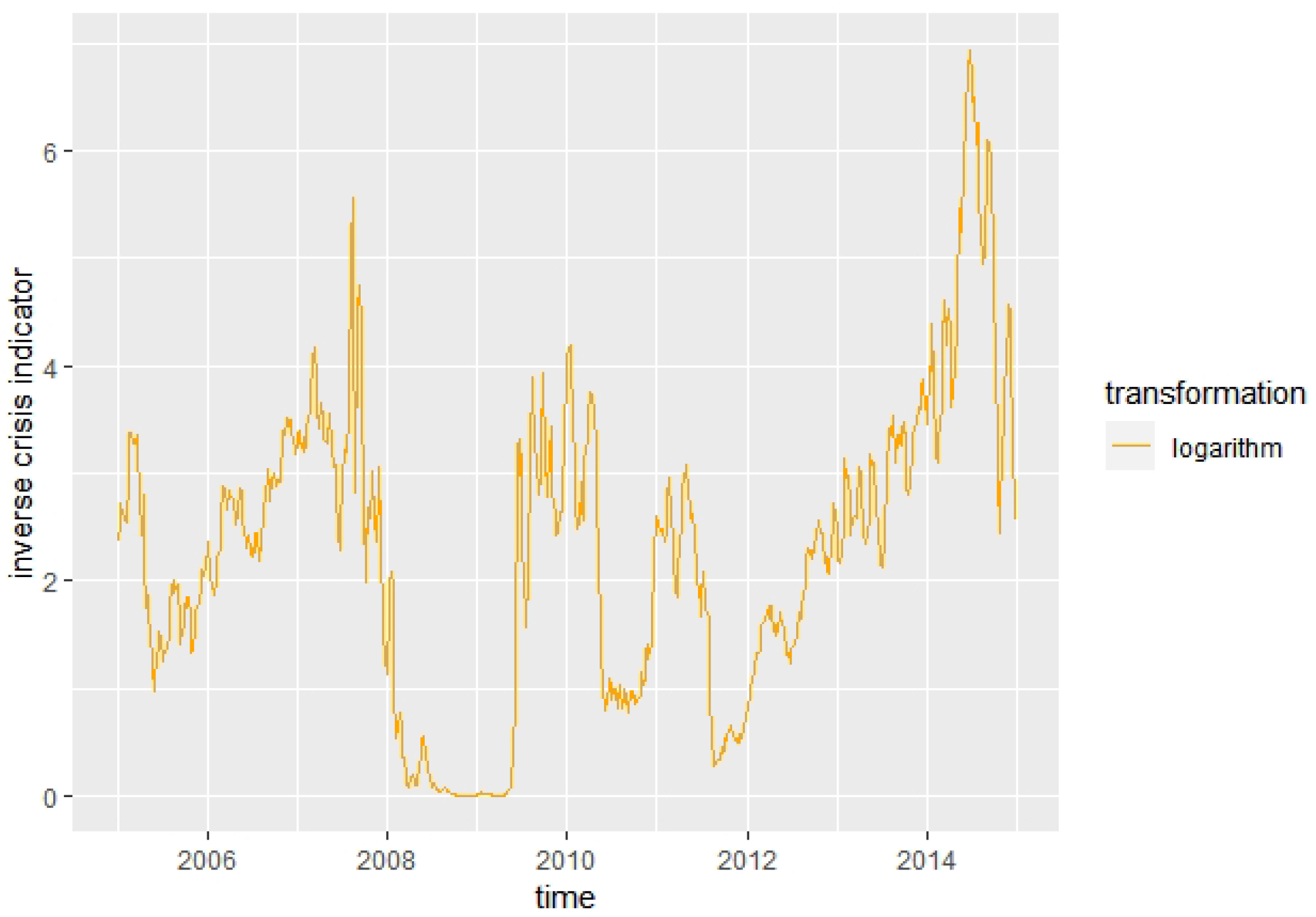
Figure 1. Log-transformation of p ( t ) .
Mathematics 13 02664 g001
Figure 2. Observed market indicator.
Mathematics 13 02664 g002
Figure 3. Simulated market indicator.
Mathematics 13 02664 g003
Figure 4. Rank of market indicator compared to 100 simulations.
Mathematics 13 02664 g004
Figure 5. Predicted volatility by model vs. observed volatility.
Mathematics 13 02664 g005
Figure 6. Observed returns.
Mathematics 13 02664 g006
Figure 7. BS: simulated returns.
Mathematics 13 02664 g007
Figure 8. C = 0 : simulated returns.
Mathematics 13 02664 g008
Figure 9. ρ = 0 : simulated returns.
Mathematics 13 02664 g009
Figure 10. Rank of risky asset compared to 100 simulations for each model. The red lines indicate the 5 % and 95 % -auantiles of the ranks.
Mathematics 13 02664 g010
Figure 11. Rank of risky asset compared to 100 simulations for each model. The red lines indicate the 5 % and 95 % -auantiles of the ranks.
Mathematics 13 02664 g011
Figure 12. F = 0 , δ = 5 .
Mathematics 13 02664 g012
Figure 13. F = 60 , δ = 5 .
Mathematics 13 02664 g013
Figure 14. F = 0 , δ = 5 .
Mathematics 13 02664 g014
Figure 15. F = 60 , δ = 5 .
Mathematics 13 02664 g015
Figure 16. Reaction of investment rate to asset development for F = 0 , δ = 5 .
Mathematics 13 02664 g016
Figure 17. Reaction of investment rate to crisis indicator X ( t ) for F = 0 , δ = 5 .
Mathematics 13 02664 g017
Figure 18. Contribution of mean–variance and hedging part to the investment rate for F = 0 , δ = 5 .
Mathematics 13 02664 g018
Figure 19. Adapted BS strategy vs. Indicator strategy risky investment rate for F = 0 , δ = 5 .
Mathematics 13 02664 g019
Figure 20. Adapted BS strategy vs. Indicator strategy portfolio performance for F = 0 , δ = 5 .
Mathematics 13 02664 g020
Figure 21. Investment into the risky asset for ‘Indicator C = 0 ’ and ‘Indicator ρ = 0 ’ for F = 0 , δ = 5 .
Mathematics 13 02664 g021
Table 1. Risk measures for the Indicator and BS strategy for different parameters.
δ = 10 δ = 5
Indicator C = 0 Indicator ρ = 0 BSIndicator C = 0 Indicator ρ = 0 BS
F = 0SR0.73990.74760.67680.74130.74850.6792
ASR0.58420.58620.52820.58470.58640.5286
Omega1.28871.29421.28881.28931.29461.2901
max DD10.7123%15.4132%8.4722%19.049%26.8999%15.1908%
F = 60SR0.71740.7150.66570.70540.69590.666
ASR0.58730.58750.53180.58550.57910.5358
Omega1.2811.28411.28231.2781.27931.2821
max DD5.3968%8.2812%4.0223%10.5296%16.284%7.6635%
F = 80SR0.70460.69660.65630.68470.6620.6579
ASR0.58380.57920.53120.57610.55570.5368
Omega1.27661.27851.27731.27191.271.2777
max DD3.2995%5.2187%2.397%6.7278%10.8841%4.7016%
Disclaimer/Publisher’s Note: The statements, opinions and data contained in all publications are solely those of the individual author(s) and contributor(s) and not of MDPI and/or the editor(s). MDPI and/or the editor(s) disclaim responsibility for any injury to people or property resulting from any ideas, methods, instructions or products referred to in the content.