Article

Numerical Optimization of Neuro-Fuzzy Models Using Evolutionary Algorithms for Electricity Demand Forecasting in Pre-Tertiary Institutions

by
Stephen O. Oladipo
1,*,
Udochukwu B. Akuru
1,* and
Ogbonnaya I. Okoro
2
1
Department of Electrical Engineering, Tshwane University of Technology, Pretoria 0183, South Africa
2
Department of Electrical/Electronic Engineering, Michael Okpara University of Agriculture, Umudike 440101, Nigeria
*
Authors to whom correspondence should be addressed.
Mathematics 2025, 13(16), 2648; https://doi.org/10.3390/math13162648
Submission received: 12 July 2025 / Revised: 11 August 2025 / Accepted: 13 August 2025 / Published: 18 August 2025

Abstract

Reliable electricity supply in educational facilities demands predictive frameworks that reflect usage patterns and consumption variability. This study investigates electricity-consumption forecasting in lower-to-middle-income pre-tertiary institutions in Western Cape, South Africa, using adaptive neuro-fuzzy inference systems (ANFISs) optimized by evolutionary algorithms. Using genetic algorithm (GA) and particle swarm optimization (PSO) algorithms, the impact of two clustering techniques, Subtractive Clustering (SC) and Fuzzy C-Means (FCM), along with their cogent hyperparameters, were investigated, yielding several sub-models. The efficacy of the proposed models was evaluated using five standard statistical metrics, while the optimal model was also compared with other variants and hybrid models. Results obtained showed that the GA-ANFIS-FCM with four clusters achieved the best performance, recording the lowest Root Mean Square Error (RMSE) of 3.83, Mean Absolute Error (MAE) of 2.40, Theil’s U of 0.87, and Standard Deviation (SD) of 3.82. The developed model contributes valuable insights towards informed energy decisions.

1. Introduction

Among several factors that determine the socio-economic state and condition of a nation, energy availability stands out as an indispensable tool. It is expected that emerging economies will account for nearly 90% of the increase in global energy demand by 2035, due to their rapid industrialization and rising living standards [1]. Consumption of energy is essential for strategic planning towards achieving the global sustainable energy program [2,3]. When a nation continues to experience inadequate supply or access to energy, the technological advancement of such a nation will nosedive. Also, the advancement in Internet of things (IoT) rides on the wings of adequate energy supply and stability. As the world’s population grows and cities expand alongside technological progress, people have increasingly relied on energy sources like oil, gas, solar, wind, coal, and many other sources to meet their rising demands [4]. Over the past decade, sustained economic growth in South Africa (SA) has steadily increased electricity demand, placing mounting pressure on Eskom’s capacity and progressively reducing its reserve margin. SA is positioned as one of the largest coal-producing nations, ranking seventh position and producing 80% of its energy from coal [5]. The effect of over-relying on coal contributes to adverse effects on the environment, making the air more polluted, accelerating climate change, and threatening both human health and ecological balance. The development of adequate energy management is crucial for citizenry since wasteful electricity consumption contributes to unnecessary electricity expenditure bills, load shedding, and negative environmental impacts [6]. Consequently, intelligent forecasting is required to consider the hemispherical seasonal dependency of energy consumption [7,8].
Alternative energy sources have grown significantly in number as the global energy demand in buildings continues to grow on a year-over-year basis. The increasing number of plug-in appliances in homes and the increased number of homes with electricity has contributed to the increasing demand for sustainable energy production and green energy [9,10]. This is also applicable to educational buildings which require many energy-consuming plug-in appliances such as office electronic equipment, space-cooling equipment, laboratory equipment, and many other energy-consuming objects. As shown in Figure 1, a common practice in recent times is to integrate renewable sources like solar, wind, and biomass into the power system of educational buildings, coordinated through a central control system. To manage this setup efficiently, it is important to forecast the building’s energy needs accurately. Without this, energy could be wasted or fall short. A smart forecasting system helps balance supply and demand in real time, allowing institutions to not only consume but also produce and share energy, thereby making them more efficient, sustainable, and part of a smarter energy future.
Known for its energy-intensive economy, SA recently experienced scheduled load shedding because of excess electricity demand. Educational institutions and the commercial sector account for approximately 10% of total electricity consumption in the country [7]. In addition, affordability remains a significant challenge, with 43% of South Africans allocating over 10% of their net income to energy expenses [11]. Considering factors such as previous consumption patterns, weather conditions, and economic trends necessitates a comprehensive analysis of electrical load demand. This is becoming even more important, as historical data often reveals how seasonal shifts, usage patterns, and factors such as temperature and humidity significantly influence demand fluctuations [12].
Exploring the potentials of data-driven machine learning (ML) models is essential when considering the complexity and changeability of power-consumption patterns. The influence of the continuous changes in weather, impact of renewable integration, and users’ behavior means that traditional statistical methods often fall short in capturing non-linear relationships and adapting to dynamic data environments. As shown in Figure 2, there has been a growing interest and advancement in modern ML, causing a shift from traditional methods. This is because modern MLs are capable of learning from vast historical datasets to provide more accurate and robust predictions, which can aid better decision making for utilities and consumers and enhance load management and optimized energy distribution.

1.1. Related Works

Previous works have carried out some research on modeling electricity consumption using conventional methods such as Autoregressive Integrated Moving Average (ARIMA), a technique for managing time-dependent data and seasonality, as well as Seasonal ARIMA, which is specifically for data that have seasonal components [13]. Various other methods and techniques have also been explored, such as k-Nearest Neighbors (k-NN), polynomial regression, multiple linear regression (MLR), exponential smoothing, decision trees (DT), regression-based models, Kalman filters, Gaussian Processes (GP), etc. For instance, Meer et al. [14] carried out a study by applying GP for probabilistic forecasting of household energy use while testing a variety of covariance functions and dynamic training. The dynamic approach reduced computation time and yielded a better result than its counterpart. Also, Kim et al. [15] presented a bottom-up electricity-demand-forecasting approach using time-series clustering of AMI data, employing Euclidean and dynamic time warping (DTW) distances. Forecasting was performed using models including ARIMA, ARIMAX, and other methods. Results showed that clustering improved prediction accuracy over total demand forecasting, and incorporating exogenous variables like humidity, insolation, and cooling degree days further enhanced model performance. Ramos et al. [16] explored how artificial neural networks (ANN) and k-nearest neighbors can be used to predict building energy consumption in different five-minute intervals, with decision trees helping choose the most suitable method for each context. By analyzing sensor data and adjusting parameters, the study shows that using DTs can significantly improve the accuracy and reliability of energy forecasts. Other studies are reported in [17,18,19,20]. The problem of forecasting electricity usage, however, is usually a time series with multiple variables, and sensor-generated data often contain gaps or missing entries, uncertainties, and redundancies that do not capture the interrelationship between different types of users [21]. Consequently, conventional methods may become incapable of handling non-linearity, uncertainty, and high-dimensional data. Modern approaches such as artificial neural networks (ANN), long short-term memory networks (LSTM), convolutional neural networks (CNN), and so on, have gained a lot of attention in the research community in recent decades. For instance, Tarmanini et al. [22] utilized two different models, namely, ARIMA and ANN to predict daily electricity demand using data from 709 Irish households over 18 months. The authors reported that better performance was obtained by ANN for the non-linear load patterns compared to its counterpart, ARIMA using mean absolute percentage error (MAPE) performance metrics. In another study, by Mohammed et al. [23], an improved ANN model using an adaptive backpropagation algorithm (ABPA) was developed to enhance long-term electricity load forecasting. Results showed that the developed model outperformed the traditional ANN, regression, and RNN methods with the minimum performance metrics. Elbeltagi et al. [24] proposed an ANN-based method to accurately predict residential building energy consumption during the early design stage using simulation data from various design options. The model improved interoperability between design and simulation tools, validated for accuracy, and developed a user-friendly interface for non-experts to support energy-efficient decision making.
While ANNs are non-linear mapping structures inspired by human neurons and have been used in many fields, they sometimes underperform because they can overfit the training data, which leads to poor generalization in real-world situations [25]. Therefore, to increase modeling speed, fault tolerance, and addictiveness, ANFIS is introduced, which blends an ANN with a fuzzy inference system (FIS) [26]. Compared to previous models, it is well known that ANFIS has become significantly more capable of correlating uncertainties as a result [27]. As a result, previous works have explored ANFIS for predicting electricity usage. For instance, Ghenai et al. [28] developed accurate energy-forecasting models for an educational building using ANFIS and data from smart meters and weather records. With over 20,000 data points, the model successfully predicted energy use up to 4 h ahead, showing strong performance and reliability, which makes it useful for managing microgrids, planning energy purchases, and improving building operations. Bilgili et al. [29] applied a fuzzy-c-means-based ANFIS and LSTM models for one-day-ahead forecasting of renewable electricity generation. According to the results obtained, both models were accurate, with geothermal showing the lowest MAPE at 1.63%, and their performances were comparable across all sources, indicating their effectiveness as short-term energy planners. Rathor et al. [30] carried out a study on three ANFIS-based models for short-term load forecasting (STLF) in the Rajasthan region of India, covering prediction intervals ranging from 15 min to one week ahead. The models outperform traditional ANN-based methods in accuracy, as demonstrated through comparative evaluation using diverse performance metrics across 15 forecasting samples.
Table 1 summarizes the previous works as discussed, along with their various contributions and areas of application.

1.2. Research Gap and Motivation

While the critical need for reliable electricity in educational buildings has led many previous studies to explore a range of standalone machine learning models like ANNs and ANFISs, these approaches often fall short due to their susceptibility to local optima and lack of parameter optimization [34]. This study addresses this fundamental limitation by establishing that the superior predictive power and robustness required for accurate consumption forecasting is best achieved through a hybrid approach. We uniquely demonstrate the effectiveness of using evolutionary algorithms (EAs) to optimally tune ANFIS parameters, moving beyond conventional methods to create a more sophisticated and reliable predictive model. This forms one of the key motivations of the present study, where we develop a hybrid model that integrates well-known EAs with ANFISs to create an effective predictive soft computing technique. Our findings indicate that the application of EA-based ANFIS models remains limited. Furthermore, many studies have overlooked the impacts of clustering techniques and hyperparameter settings on the performance of the developed models. Selecting an appropriate clustering technique is crucial for achieving efficacy and ensuring high-quality prediction accuracy. Ultimately, model accuracy will suffer if clustering methods and hyperparameters are not carefully chosen.
The choice of genetic algorithm (GA) and particle swarm optimization (PSO) algorithm to optimize the parameters of the ANFIS is based on their robust nature, especially because they do not require gradient information, which is a significant advantage over classical optimization methods. Compared to many other metaheuristic algorithms, GA is recognized for its global search capability which aids its exploration of a large search space in order to avoid becoming trapped in local minima. In addition, inspired by natural selection, GA iteratively evolves a population of potential solutions through processes like parent selection, crossover, and mutation, enabling it to handle a wide variety of non-linear problems with both continuous and discrete variables. Consequently, the hybridization of GA and ANFIS creates a model that harnesses GA’s optimization prowess with ANFIS’s learning capability to improve prediction accuracy and reduce error rates.
Similarly, the choice of PSO is based on its simplicity, computational efficiency, and fast convergence rate. PSO mimics the social behavior of bird flocks and fish schools. In its operation, each particle’s movement is guided by its own best-known position and the swarm’s best-known position, allowing it to quickly find a good solution. Combining PSO with ANFIS provides a synergy that allows PSO to optimally tune the ANFIS parameters, which is particularly effective in problems with continuous variations.
This study evaluates the performance of ANFIS models optimized by PSO and GA. It investigates the use of Subtractive Clustering (SC) and Fuzzy C-Means (FCM) to forecast electricity consumption in low-to-middle-income pre-tertiary schools, with a special focus on the Western Cape region of South Africa. The developed hybrid models were tested on two schools, referred to as Case A and Case B. Consequently, this led to the development of several sub-models. The best performing parameter combinations for each clustering method were chosen for both PSO-ANFIS and GA-ANFIS models based on their accuracy, and the overall top model for each output was selected using the lowest error values. The model’s operation stems from the fusion of ANN relational structures and learning skills, fuzzy logic’s intrinsic dynamic qualities in decision making as embodied in ANFIS, and the parameter-tuning capabilities of EAs.
The main contribution of this study is to develop two evolutionary-based adaptive neuro-inference systems for electricity forecasting in lower-to-middle-income pre-tertiary education institutions. The developed hybrid models were tested on two schools, referred to as Case A and Case B. Consequently, this led to the development of about 48 models. In addition, this study also investigates the effect of two renowned clustering techniques namely SC and FCM as well as other pivotal hyperparameters on model accuracy. Finally, it identifies the optimal model and compares it with three different variants including stand-alone ANFIS and other hybrid models.

1.3. Contributions of the Study

The main contributions of this study are as follows:
  • It develops two evolutionary-based adaptive neuro-inference systems for electricity forecasting in lower-to-middle-income pre-tertiary education institutions;
  • It investigates the effect of two renowned clustering techniques, namely subtractive clustering and fuzzy c-means, and other pivotal hyperparameters on model accuracy;
  • It identifies the optimal model and compares it with three different variants, stand-alone ANFIS, and other hybrid models.
The rest of this study is structured as follows: Section 2 details the materials and methodology employed; Section 3 presents and discusses the experimental results; Section 4 offers the conclusion and outlines potential directions for future research.

2. Materials and Methods

2.1. Data

Located in the southernmost part of Southern Africa, the Western Cape Province is known for its manufacturing, construction, mining, and agriculture industries [35]. The Western Cape, South Africa’s fourth largest province, lies in the country’s south-western corner, bordered by the Northern Cape to the north, the Eastern Cape to the east, the Atlantic Ocean to the west, and the Indian Ocean to the south [36]. The Western Cape has a Mediterranean climate with warm, dry summers and cool winters, but its rainfall can be unpredictable, making it one of South Africa’s driest areas with only about 350 mm of rain a year [35]. The data used for this experiment were obtained from [37]. The data were captured by smart meters, cleaned, and pre-processed to ensure precision and accuracy. They covered 53 schools, spanning the period from 1 December 2022 to 30 November 2023. The raw data are available in [37]. This study focused on two lower-to-middle-income public primary and secondary schools in the Western Cape, South Africa. The two schools were selected from the low economic quintile. The Western Cape features three main rainfall patterns: winter rainfall, late summer rainfall, and areas with consistent rainfall throughout the year [38]. We used one month of weather data, specifically for July, as it is one of the coldest months with average daily highs of around 17 °C and average lows of 7 °C. The month is also characterized as being the wettest month with frequent cold fronts and storms. The climatic data for the study area were sourced from Open-Meteo Historical Weather. Figure 3 illustrates the architectural design of the model.
Economic quintiles are used to classify public schools based on the relative poverty of the communities they serve in South Africa. This classification helps the government allocate funding and resources equitably. This study selected two schools from Quintiles 1 and 2 (Table 2). Case A, which is a school under Quintile 1 Schools (Q1), represents the poorest 20% of schools in the country. Schools under the Q1 category are typically located in rural or underdeveloped areas with communities with very low household incomes and limited infrastructure. In addition, learners are not required to pay school fees, and the government provides additional financial support. In many cases, they are faced with greater challenges in terms of infrastructure, teaching resources, and learner support. The second school (Case B) utilized in this study is categorized under Q2. Q2 represents the second-poorest 20% of schools. Similar to Q1, they are no-fee schools, with similar support structures as Quintile 1. Although, slightly better off than Q1 schools, they also serve economically disadvantaged communities. However, in contrast with Q1 schools, they may have modestly better infrastructure or access but still require substantial government support to meet learner needs.
Given the conditions of the schools, developing an effective model for predicting energy use becomes essential in order to improve energy management and operational planning. In addition, this can help equip the pre-tertiary institution with practical tools to manage limited resources, reduce waste, and enhance both educational and operational outcomes.

2.2. Adaptive Neuro-Fuzzy Inference System

A neuro-fuzzy inference system combines the learning abilities of ANNs with fuzzy inference systems (FISs) to mimic expert decision making [38]. In ANFIS modeling, fuzzy rules connect the antecedent and consequent components of the Takagi-Sugeno inference fuzzy system. ANFIS combines the least-squares method with the backpropagation gradient descent algorithm, using the former to fine tune the linear output parameters and the latter to adjust the non-linear premise parameters tied to the fuzzy membership functions [39]. In the forward-learning phase, the least-squares method keeps the premise fixed while fine tuning the consequent parameters. Once the best consequent values are found, the membership function parameters in the premise are then adjusted using the gradient descent method during the back-learning phase. ANFIS parameters fall into two categories: the linear ones found in the consequent part and the non-linear ones located in the premise part. For a fuzzy inference system (FIS) with two inputs, x and y, and one output F, the relationships shown in Equations (1) and (2) outline the rule base—essentially, the set of fuzzy logic rules that guide the system’s decision making.
Rule   1 :   If   x is   I 1 and   y is   J 1 , F 1 = a 1 x + b 1 y + c 1
Rule   2 :   If   x is   I 2 and   y is   J 2 , F 2 = a 2 x + b 2 y + c 2
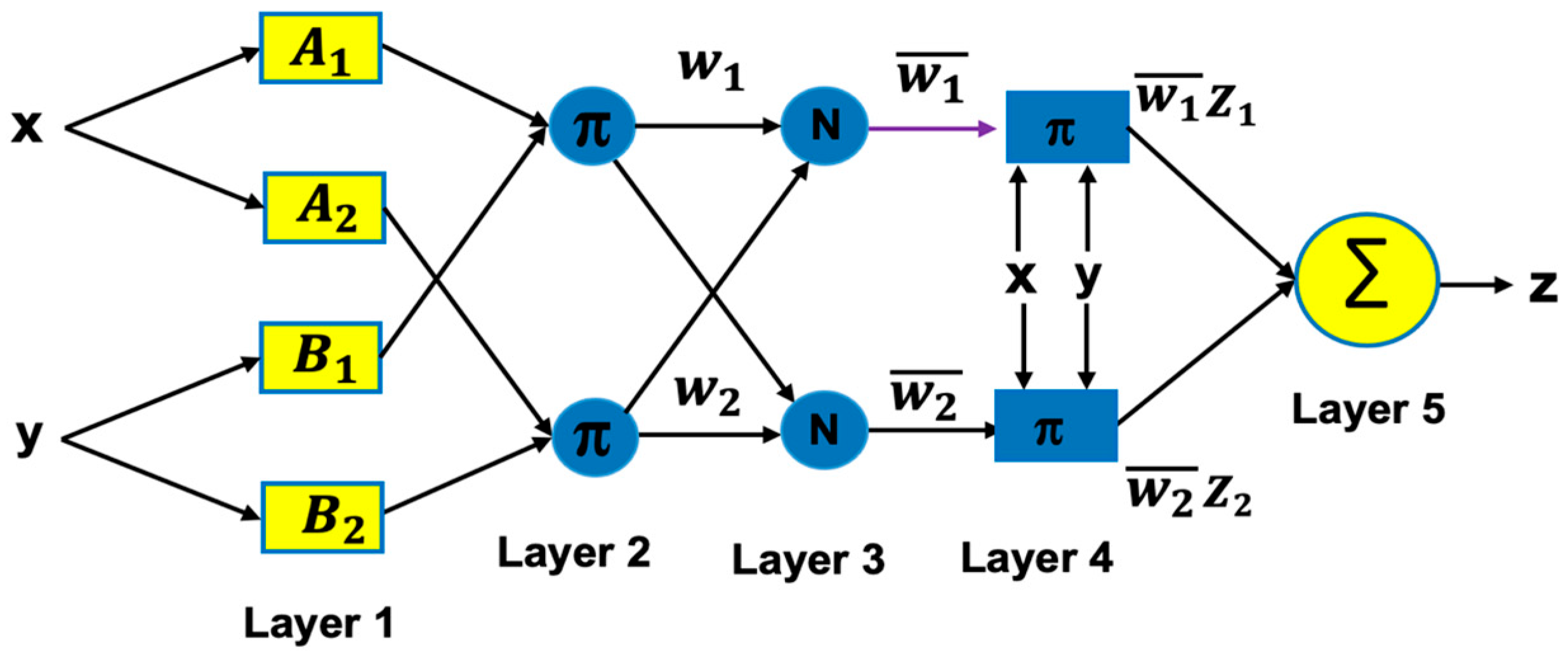
In this case, the membership functions are labeled I 1 , I 2 , J 1 , and J 2 , with x and y as the input variables and F 1 and F 2 as the system outputs. The consequent parameters at the nodes are represented by a, b, and c. Figure 4 illustrates the ANFIS structure, which consists of five layers: the first handles the inputs, the second performs fuzzification, the third and fourth evaluate the fuzzy rules, and the fifth carries out defuzzification to produce the final output.
The ANFIS model is built with five layers—fuzzy, product, normalization, defuzzification, and output—as shown in Figure 2. While the product, normalization, and defuzzification layers have a fixed number of nodes, the fuzzy and output layers are adaptive, meaning their nodes can be adjusted based on the model’s parameters. In the first layer, each adaptive node corresponds to a fuzzy membership function, and the final output is determined by the following function:
O j 1 = μ A j ( I 1 ) ,                       j = 1,2
O j 1 = μ B j ( I 2 ) ,                       j = 1,2
Also, the second layer contains fixed nodes, and the firing strength of each rule is determined using Equation (5).
O j 2 = w j = μ A j I 1 × μ B j I 2 ,                     j = 1,2
The third layer adjusts the firing strength at each node by normalizing it—essentially dividing the firing strength of a given node by the total firing strength of all nodes, as shown in Equation (6). The resulting values for both the normalized layer and firing strength range between 0 and 1.
O j 3 = w i ¯ = w j w 1 + w 2 ,                       j = 1,2
This layer carries out the defuzzification process, where each node is adaptive and uses learned functions. These nodes combine the inputs with the normalized signals from the previous layer to determine how much the jth rule contributes to the final output, as shown in Equation (7).
O j 4 = w j ¯ z j = w i ¯ p j I 1 + q j I 2 + r j
where p j , q j , and r j are the consequent parameters of the node j .
The fifth layer contains fixed nodes that use a summation function to combine all the incoming signals from the previous layers [40].
O j 5 = j w j ¯ z j = j w j z j j w j

2.3. Clustering Methods

Clustering can be referred to as a way of simply grouping similar pieces of data together in order to allow for more organization and meaningfulness. This phenomenon plays a significant role in data analysis and has a huge impact on the performance of the ANFIS model. In this study, we used two different clustering methods to sort the data into fuzzy groups, which then helped define the MFs and build the structure of the FIS. The two methods we relied on are Fuzzy C-Means (FCM) and Subtractive Clustering (SC), both widely used for this kind of task.

2.3.1. Fuzzy C-Means Method

Fuzzy c-means is a well-known clustering method often used in ANFIS modeling, allowing each data point to be shared among multiple clusters. It works by assigning membership values based on how far a point is from the center of each cluster. The application of FCM has gained a lot of attention in the research community due to its unsupervised capabilities in the analysis of data and building of models. Some of the areas where FCM has been explored are agricultural engineering, image analysis, astronomy, chemistry, and medical diagnostics [41]. As a clustering-based problem, determining the membership function (MF) is vital to ANFIS. The primary purpose of the FCM technique is to reduce the total number of fuzzy rules used in the analysis. The application of the FCM technique paves way for determining the extent to which data belong to different clusters by minimizing the objective function. Equation (9) is used to calculate the best possible distance between each data point x i and the center of its fuzzy group, for every group n.
E = i = 1 N k = 0 n U i j m x i c j 2
Here, m is the weighting exponent that falls within the range of 1 to infinity; U i j m shows how strongly a data point x i belongs to cluster j, with values between 0 and 1. The center of each cluster is labeled c j , and C stands for the total number of clusters. The value of U i j for a data point in cluster j at any step of the process is calculated using:
U i j = k = 1 C x i c j x i c j 2 m 1 1

2.3.2. Subtractive Clustering (SC) Method

In Subtractive Clustering (SC), it is assumed that there is a possibility that every data point could become the center of a cluster. Based on the density of the data points directly surrounding the cluster center, it determines the probability of each point defining the cluster center [42]. Assuming the process of combining the system’s input dataset X with its output dataset Y, the resulting dataset is denoted as x . If each feature in x has been normalized, the entire set fits within a defined space—specifically, a hypercube. SC then evaluates every point as a possible cluster center by measuring distances between them, using Equation (11) below [43].
D i = j = i n e x p x i x j 2 r a 2 2
The symbol r a represents the radius of each cluster, |.| stands for the Euclidean distance between points, and n refers to the total number of data points. Using the SC algorithm, the potential of each point is first calculated with Equation (12). The initial cluster center, x c 1 , is selected as the point with the highest potential, labeled D c 1 . After that, the potential of every data point x i is adjusted based on the following equation [43]:
D i = D i D c 1 e x p x i x j 2 r a 2 2
where r b represents the radius around each cluster where the potential starts to drop off significantly. To avoid placing clusters too close to each other, r b is usually set larger than r a [44]. When selecting the next cluster center, the point with the highest remaining potential is chosen. This process continues until one of the stopping conditions is met.
The clustering techniques are integrated into the ANFIS structure to automatically generate the initial fuzzy rules and membership functions from the dataset. This process partitions the input–output data space into meaningful clusters, where each cluster corresponds to a fuzzy rule. The center and spread of these clusters are used to define the parameters of the membership functions, providing a data-driven and efficient alternative to manual rule creation. This structured initialization then allows the ANFIS’s hybrid learning algorithm to fine tune the membership function and consequent parameters, resulting in a more accurate and robust model.

2.4. Evolution-Based Soft Computing for ANFIS

Evolutionary algorithms are a class of computational methods that mimic genetic improvements in humans and the natural behavior of animals, operating on the principle that the fittest individuals in a population are more likely to survive and succeed when resources are limited [44]. The present study harnessed the effective capabilities of two renowned evolutionary algorithms, namely, genetic algorithm (GA) [45] and particle swarm optimization (PSO) [46] algorithm, to optimize the structure of ANFIS for electricity prediction. The next sessions discussed how the models were developed.

2.4.1. Genetic Algorithm-Based ANFIS

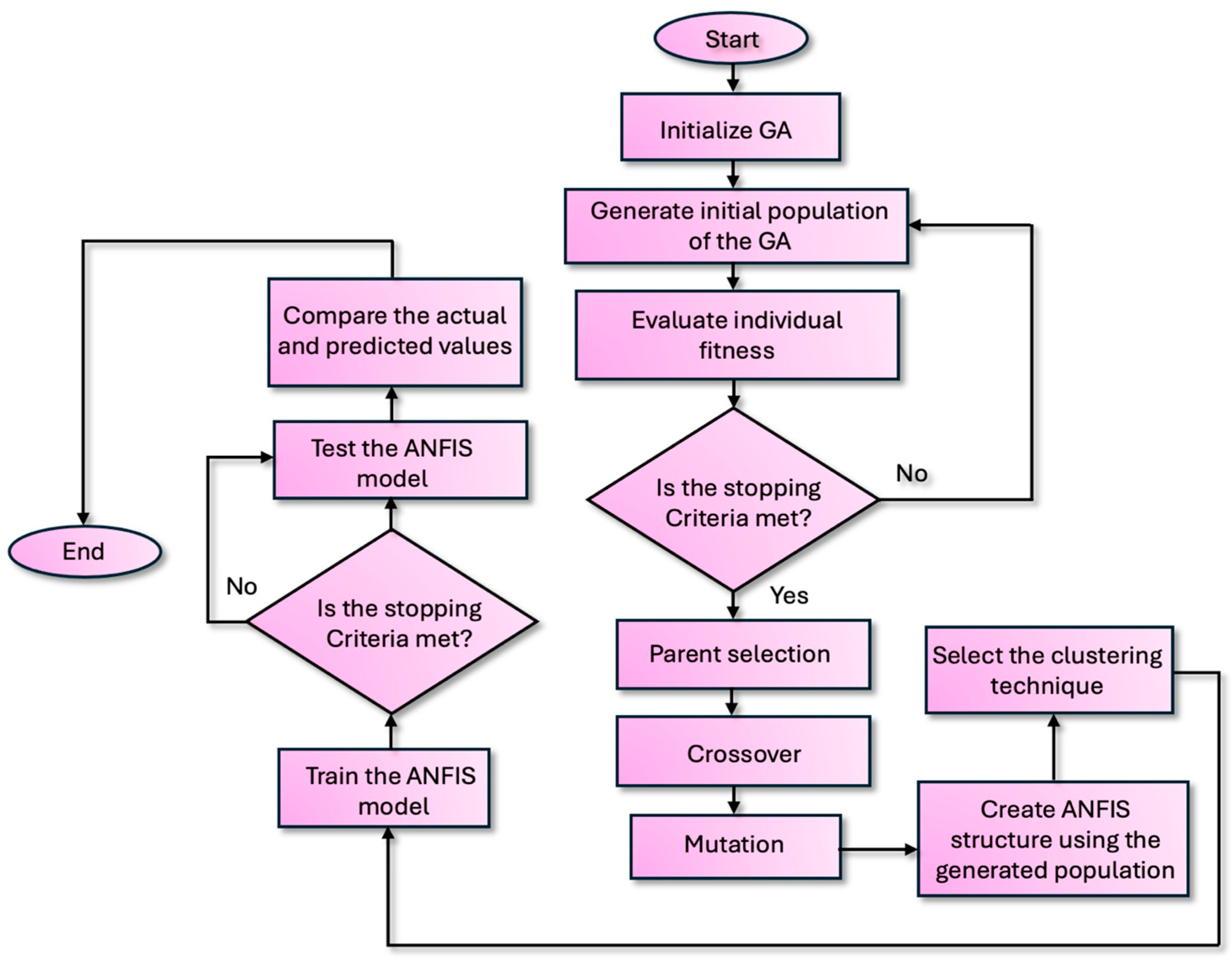
Genetic algorithm was first introduced by J. H. Holand [45]; since then, it has been an algorithm of choice for several researchers and has been used in different spheres of application. GA is known to mimic nature’s survival of the fittest mechanism in accordance with Darwinian theory. The amalgamation of GA and ANFIS produces a hybrid model that harnesses the optimization prowess of GA with the learning capability of ANFIS. As a result of optimizing the Sugeno-based FIS membership function, the fusion improves prediction accuracy and reduces error rates [47]. Figure 5 presents the flowchart of the GA-AFNIS. The process starts with the initialization of the algorithm. This is followed by the generation of its population, which represents a set of potential solutions. Depending on the predefined criterion, each individual within this population then goes through an evaluation of its fitness. The GA iteratively progresses with parent selection, crossover, and mutation operations to evolve the population, continuously seeking improved solutions until its specific stopping criteria are met.
When the GA stopping criteria are met, the process transitions to the ANFIS design stage. At this stage, the optimal or near-optimal parameters derived from the generated population of GA are utilized to create the ANFIS structure. Concurrently or prior to this, a clustering technique is selected to help in defining the initial configuration of the fuzzy rules and the MFs within the ANFIS. Afterwards, the ANFIS model goes through the training stage where the internal parameters are adjusted to learn from the data. This training continues iteratively until the ANFIS model’s own stopping criteria are satisfied. Finally, the trained ANFIS model is rigorously tested, and its predicted outputs are compared against the actual values to assess its performance under different performance metrics.

2.4.2. Particle Swarm Optimization-Based ANFIS

Kennedy and Eberhart [46] introduced PSO, a widely recognized evolutionary algorithm inspired by the natural movement patterns of bird flocks and fish schools. Since its introduction, this population-based, nature-inspired method has earned broad acceptance and has been successfully applied in many fields. The study utilized PSO to tune the parameters of ANFIS, yielding a hybrid model for electricity prediction in educational institutions. As described in Figure 6 the simulation begins with the initialization of the PSO algorithm, followed by the generation of the initial swarm of particles. Each of the particles represents a potential solution. After this, the fitness of all the particles is then determined, and their individual local optimal fitness values are carefully recorded. The process continues by performing a check to see if any of the particle’s current fitness value is superior to the best overall fitness found so far. If that is the case, the new best fitness becomes the global best. Following this, the velocities and positions of all the particles are updated, and the fitness re-evaluated, continuing the iterative optimization search inherent to PSO.
After some time, a check is performed to see if the stopping criteria are not met and the decision is taken accordingly. If these criteria are met, the PSO optimization continues to refine the particle positions. If the stopping criteria are not met, the current best fitness obtained from the PSO phase is then utilized as input for the ANFIS. However, before training the ANFIS model, a clustering technique is selected, a step which is highly essential in determining the initial structure of the FIS. After this, the ANFIS model goes through the training phase, during which its parameters are adjusted. This training continues iteratively until its own specific stopping criteria are met. Once the training stage is successfully implemented, its performance is evaluated by comparing its predicted values against the actual values, thereby assessing its accuracy and generalization capabilities under the performance metrics. The entire process ends after the final evaluation. The following explains how velocity and position are defined. Given that each particle i in N population consists of an X i d position component and a V i d velocity component at the d t h dimension, the position and velocity updates of each particle can be expressed as follows:
v i t + 1 =   w   v i t +   c 1 r 1 ( p b e s t   x i t )   +   c 2 r 2 ( g b e s t   x i t )
x i t + 1 = x i t + v i t + 1
The variables r 1 and r 2 represent random numbers within the range of [0, 1], while c 1 and c 2 denote the cognitive and social constants, correspondingly. The term w is the inertia weight. Figure 4 shows the PSO-ANFIS model used.

2.5. Model Performance Evaluation

To evaluate the performance of the developed model, it is important to assess it using specific performance metrics. Both the models and sub-models were rated based on four statistical metrics outlined in Equations (15) and (16). To ensure a fair comparison and test the reliability of the models, all analyses used the same set of metrics. The performance metrics shown in Equations (15) and (16) help to provide insights into the robustness, reliability, and accuracy of the developed model. For instance, RMSE reveals the error of the predictive model by heavily penalizing large deviations. The lower, the better. The MAE shows the magnitude of the error between the predicted and actual values of the developed models. MADE and SD reveal the variability of electricity data. Higher values suggest more fluctuations and potential difficulties in prediction. Theil’s U coefficients compare the performance of the predictive model to a naïve forecast. If Theil’s U < 1, then that model offers superior predictions over simple historical averages. It is noteworthy that the lower values across these metrics indicate that the model provides more precise, consistent, and dependable electricity-forecasting performance. Mathematical descriptions of the performance-evaluation metrics are presented in Equations (15) and (16):
Root Mean Square Error:
R M S E = 1 N i = 1 N y k y ^ k 2
Mean Absolute Deviation Error:
M A D E = 1 N k = 1 N y k y ¯  
Standard Deviation:
S D = k = 1 N y k y ¯ 2 N 1
Theil’s U:
Theil s   U   =   1 N i = 1 N y k y ^ k 2 1 N i = 1 N y k 2 + 1 N i = 1 N s y ^ k 2
Mean Absolute Error:
M A E = 1 N k = 1 N y k y ^ k
where k is the sample index and y k and y ^ k are the actual and predicted values, respectively; Y ¯ is the average of the actual values.

3. Results and Discussion

The following section presents the output of the developed models and the statistical analysis of the results. The models were implemented on a Microsoft Windows 11 operating system, utilizing an Intel (R) @2.59 GHz processor and 32 GB of RAM. Two low-to-middle-income pre-tertiary educational institutions are used. A 30% hold-out dataset was used to assess the model’s performance. Within the research framework, the impact of clustering techniques and hyperparameters is comprehensively tested using the hybrid models, resulting in several sub-models.
The ANFIS structure utilizes two different clustering methods to organize the data into similar fuzzy clusters, which are then used to assign membership functions (MFs) and generate the fuzzy inference structure from the data. Two renowned clustering techniques, namely Subtractive Clustering (SC) and Fuzzy C-Means (FCM), are employed in this study. The two pre-tertiary educational institutions are designated as Case 1 and Case 2. The models developed using each clustering algorithm are applied to forecast electricity consumption. To determine the optimal number of clusters, a range of values from 2 to 6 was tested. This is crucial, as the optimal selection influences the number of rules and membership functions, which in turn affects the precision of the FCM-based models. The clustering approach aims to group data based on similarity scores. The SC technique assumes that each data point has the potential to become the nucleus of a cluster. Accordingly, a range of cluster radius (CR) values from 0.3 to 0.7, in increments of 0.1, was tested. The parameter settings of the models are presented in Table 3.

3.1. Overview of Case Studies

This section presents detailed analyses of the developed predictive modeling applied to two pre-tertiary educational institutions. The models’ performances are evaluated using the two hybrid models, clustering techniques, and hyperparameter variations in forecasting the electricity consumption in both cases. Case A focuses on a low-income school with a larger student population, while Case B examines a combined-category school with slightly fewer students. Comparative results for both cases are discussed to identify optimal modeling strategies and parameters.

3.1.1. Case A: Evaluation of Hybrid Model Performance in Pre-Tertiary Institution A

Case A consists of a pre-tertiary institution which consists of 1405 learners and falls under the category of low-income schools. The performance of the SC-clustered GA-ANFIS model is reported in Table 4, and Figure 7 shows the performance with varying cluster radii. The evaluation of the hybrid models was carried out using five statistical metrics. As shown in Table 4, the sub-model GA-ANFIS-SC with a CR of 0.4 delivered the best performance in RMSE (5.3640), MADE (3.1917), MAE (3.2396), Theil’s U (0.8035), and SD (5.3641). The implication is that GA-ANFIS-SC with a CR of 0.4 delivered a balanced rule base, minimal prediction error, and variability. In addition, Table 4 shows that a clustering radius of 0.4 is optimal for the model, as it yields the lowest errors across all performance metrics. A smaller radius, such as 0.3, may result in an overly complex model that risks overfitting, while larger values between 0.6 and 0.7 may oversimplify the model, leading to underfitting and missed patterns in the data. This indicates that increasing the clustering radius in an SC-clustered GA-ANFIS model does not necessarily lead to improved performance. It is therefore essential to test different clustering radius values to determine the most effective one. This supports recent studies that have examined the impact of clustering techniques on model development in order to identify the best hyperparameters for hybrid models in machine learning [48,49,50].
Table 5 presents the results obtained from the FCM-clustered models. The best performance was produced by the GA-ANFIS-FCM sub-model with four clusters, achieving the lowest RMSE (5.8777), MAE (3.8117), Theil’s U (1.0097), and SD (5.8886). The implication of this is that the GA-ANFIS-FCM with four clusters resulted in fewer prediction errors compared to the other sub-models. This is clearly seen in Figure 8—using only two or three clusters resulted in underfitting, and the model was too simplistic to capture the underlying consumption patterns accurately. Conversely, increasing the number of clusters beyond four led to a decline in performance, likely due to overfitting and increased model complexity. It can be observed that increasing the number of clusters beyond four led to a decline in performance, likely due to overfitting and increased model complexity. In addition, the results showed that the use of seven clusters produced the highest error and variability, confirming that excessive partitioning may destabilize the model and reduce its predictive reliability.
Again, this substantiates the fact that increasing the number of clusters may not necessarily enhance model performance, and therefore further experiments are required to determine the optimal number of clusters.
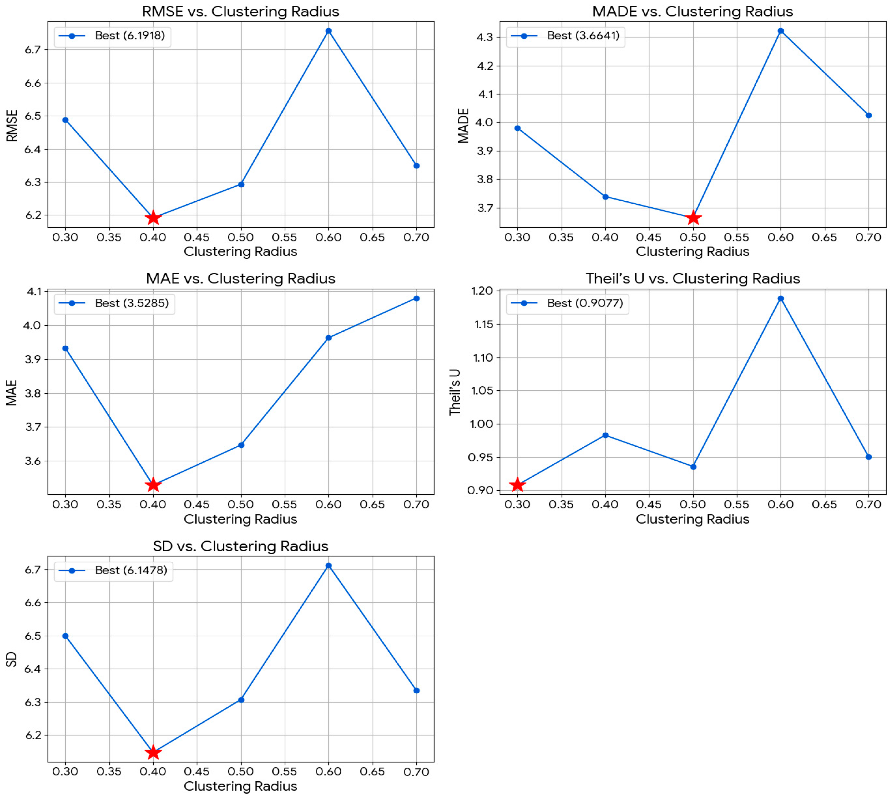
The following discusses the SC- and FCM-clustered PSO models under Case A. As shown in Table 6, the sub-model with a clustering radius of 0.4 exhibited the best performance across three key metrics: RMSE (6.1918), MAE (3.5285), and SD (6.1478). However, the sub-models with CR values of 0.3 and 0.5 demonstrated competitive performance in terms of MADE (3.6641) and Theil’s U (0.9077), respectively. Performance evaluation of the PSO-ANFIS-SC model with varying clustering radii is presented in Figure 9. It is worth noting that a model’s ability to accurately capture data patterns can be influenced by the impact of the CR on the structure and generalization capability of the fuzzy inference system. The sub-model with a CR of 0.4 appears to strike a more balanced trade-off between model complexity and accuracy across the key performance metrics. Meanwhile, the sub-models with CR values of 0.3 and 0.5 showed localized strengths in MADE and Theil’s U, as reflected in the table.
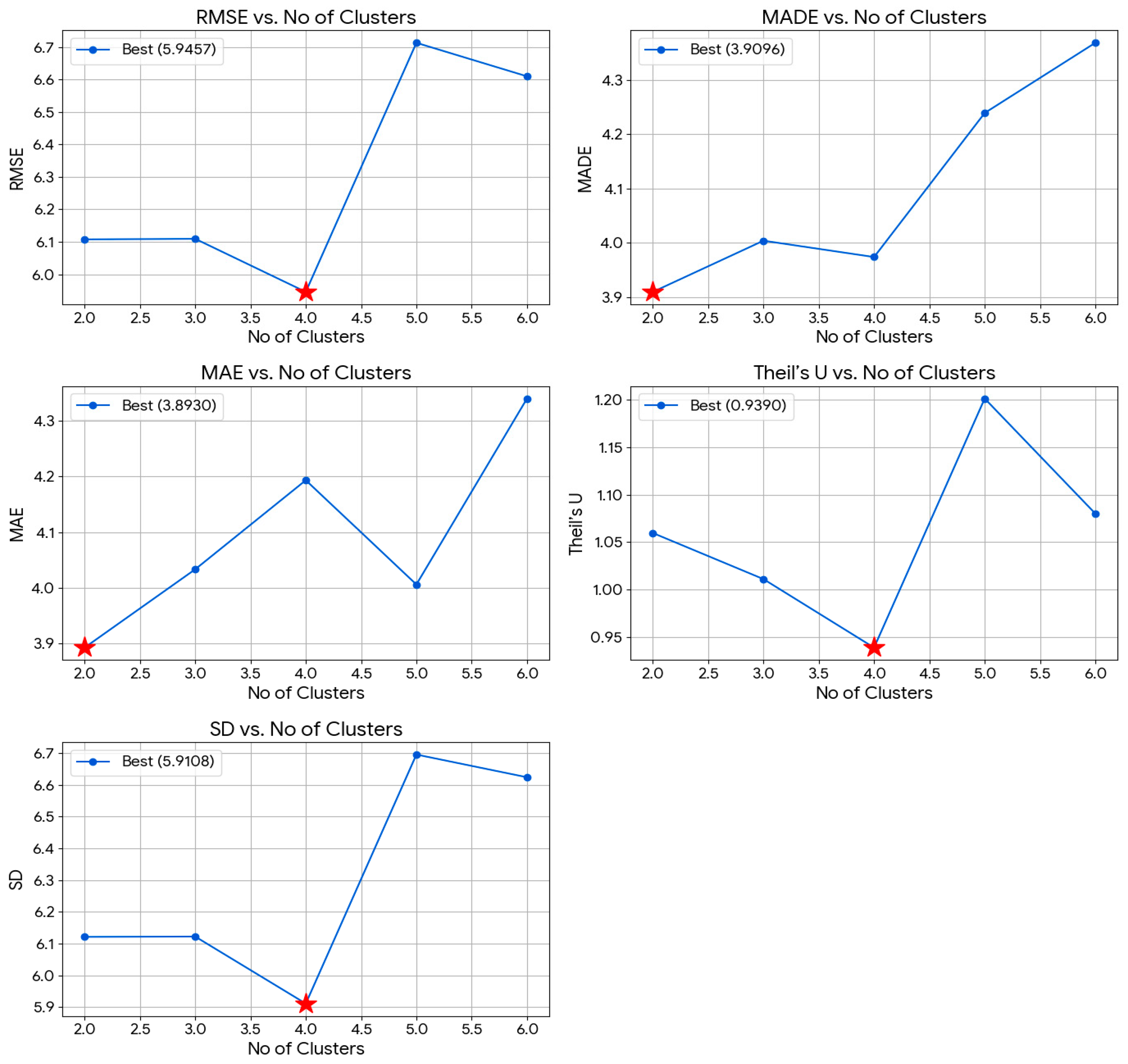
Table 7 presents FCM-clustered PSO-ANFIS for Case A. The results showed that the sub-model with four clusters surpassed other models in terms of the RMSE (5.9457), Theil’s U (0.9390), and SD (5.9108). Although the MAE was slightly higher than in the two- and three-cluster cases, the overall error profile indicates that four clusters offered the best trade-off between model complexity and predictive accuracy. In contrast, using five or six clusters led to increased error and variability, suggesting overfitting and reduced generalization capability. However, the model with two clusters delivered a competitive performance in terms of the MADE (3.9096) and MAE (3.9096). This suggests that PSO-ANFIS-FCM (with four clusters) delivered more accurate prediction of electricity usage with fewer large deviations from actual values and more stable performance, as indicated in Figure 10.

3.1.2. Case B: Evaluation of Hybrid Model Performance in Pre-Tertiary Institution B

School B, classified under the combined category, has 1159 learners. Its electricity load profile was used to develop predictive models using the same parameter settings applied to the previous school. Table 8 presents the performance of the SC-clustered GA-ANFIS model for electricity load prediction in School B. The best results were achieved by the sub-model with a CR of 0.6, which recorded the lowest RMSE (4.0090), MAD (2.3966), MAE (2.4791), and SD (4.0087). However, although Theil’s U at 0.6 (0.9110) is slightly higher than at 0.3 (0.8466), the overall error distribution favors 0.6 due to consistency and minimal spread (lowest SD). As seen in Table 8, a radius of 0.7 clearly underperforms, likely due to underfitting, where the model is too simple to capture the data’s complexity. Also, cluster radii between 0.3 and 0.5 show comparable performance, but none match the balance and stability of the model at 0.6. Generally, the GA-ANFIS-SC model with a clustering radius of 0.6 appears to be the most suitable for forecasting future electricity consumption in this category. Figure 11 shows the results of the varying clustering radii.
As reported in Table 9 and observed in Figure 12, the best performance was achieved at four clusters, where the GA-ANFIS-FCM model recorded the lowest RMSE, MADE, MAE, Theil’s U, and SD. While Clusters 2 and 5 performed moderately well, they did not match the accuracy and consistency of the four-cluster configuration. At three and six clusters, prediction error increased significantly, particularly with Theil’s U values exceeding 1, which suggests the model performs worse than a naïve forecast at those points. Overfitting and model instability are likely when the number of clusters is either too low or too high. This signifies that GA-ANFIS-SC with four clusters yielded the most accurate predictability and is able to capture complex consumption patterns.
The performance of SC-clustered PSO models for electricity prediction in School B is presented in Table 10. The best performing sub-model was PSO-ANFIS-SC with a CR of 0.6, achieving the lowest MADE (2.4102), MAE (2.4123), and Theil’s U (0.9272). While the model at 0.5 yielded the lowest RMSE and MAE, indicating high prediction accuracy, the configuration at 0.6 provided the lowest MADE and Theil’s U, suggesting more stable and consistent forecasts. Both settings outperformed the other radii across key metrics. On the other hand, increasing the clustering radius to 0.7 led to the highest prediction error and variability, reflecting underfitting and reduced model sensitivity. Therefore, a clustering radius between 0.5 and 0.6 offers the most reliable results for electricity-consumption prediction using the PSO-ANFIS-SC framework. Figure 13 shows the performance of different clustering radii in the model.
As seen in Table 11, the sub-models with fewer clusters delivered better results in the FCM-clustered models. The models with two and three clusters delivered a competitive performance compared with other models. However, the PSO-ANFIS-FCM with two clusters demonstrated a greater improvement over its counterparts with the lowest MADE (2.4928), Theil’s U (0.9194), and SD (4.1853). The other sub-model with three clusters performed slightly better in RMSE (4.1914) and MAE (2.6042). The possible cause of this is that the sub-models that utilized fewer clusters have the prospect of providing a simpler fuzzy rule base which can help improve generalization and reduce overfitting. The PSO-ANFIS-FCM model with two clusters captured the dominant trend in the data without introducing unnecessary complexity into the sub-model; while the one with three clusters marginally delivered a better fit in terms of RMSE and MAE, though at the possible cost of increased variability. The performance evaluation of the PSO-ANFIS-FCM model with varying number of clusters is presented in Figure 14.

3.2. Performance Comparison Between the Optimal Sub-Models of Case A and Case B

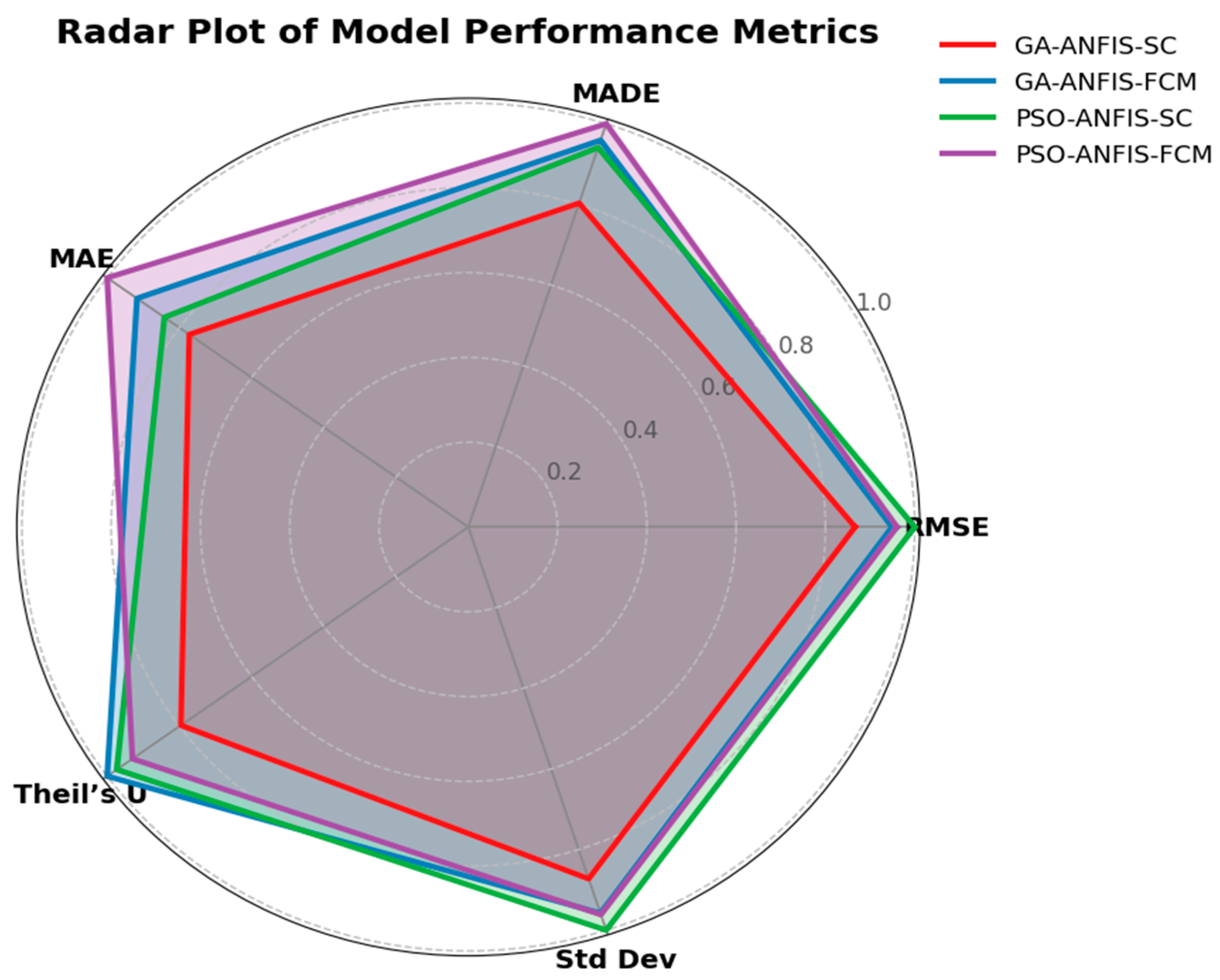
This section discusses the performances of the best optimal sub-models in both cases under different clustering techniques, hyperparameter values, and hybrid models. Table 12 reports the results of the best performing sub-models. As can be seen in Table 12, the best performing sub-models belong to the SC-clustered GA-ANFIS with a cluster radius of 0.4, with the lowest RMSE (5.3640), MADE (3.1917), MAE (3.2396), Theil’s U (0.8035), and SD (5.3641). This is also revealed in the radar plot as shown in Figure 4, which compared GA-ANFIS-SC with 0.4 cluster radius, GA-ANFIS-FCM with four clusters, PSO-ANFIS-SC with CR 0.4, and PSO-ANFIS-FCM with four clusters. It is evident from the figure (Figure 15) that GA-ANFIS-SC (cluster radius of 0.4) yielded the most balanced and superior performance across the metrics, as clearly shown by its having the smallest enclosed area on the radar plot. Nevertheless, whereas GA-ANFIS-FCM (4 clusters) also performed well in some areas, particularly Theil’s U and SD, it was overall outperformed by GA-ANFIS-SC (cluster radius of 0.4). On the other hand, the PSO-based models, though delivering a competitive result, yielded a smaller radar coverage, signifying less predictive accuracy. Figure 16 shows the relationship between the actual and predicted electricity consumption for the best optimal sub-model, i.e., GA-ANFIS-SC (cluster radius of 0.4). The figures show a close relationship between the predicted and actual electricity consumption, with some level of overlap.
The result obtained from Case A showed that the combination of GA and SC with CR of 0.4 delivered the smallest average prediction error and is capable of capturing the underlying data pattern more effectively, with the best generalization ability. The optimal performance of the model can be attributed to its use of SC, which helps to produce a compact and representative fuzzy inference system that is capable of yielding interpretability and computational efficiency. Having a moderate cluster radius of 0.4 means that the generated fuzzy inference system was neither too complex nor too simple. This strategic synergy of GA, ANFIS, and optimal number of clusters can produce a model that has good structure, better generalization, and lower prediction error as seen in the results and in this case.
Another advantage of the sub-optimal model is gained from pairing it with the SC method. This helps generate a compact and representative FIS, leading to efficacy in both interpretability and computational efficiency. A CR of 0.4 typically signifies a moderate number of clusters, which means the generated FIS was neither overly complex nor too simple, allowing the model to generalize better. Therefore, it can be concluded that the strategic combination of GA, ANFIS, and SC yielded an optimal configuration that led to a model with optimal structure, improved generalization, and lower prediction errors in this case.
In Case B, similar to Case A, the GA-optimized ANFIS with four clusters outscored its counterparts in all the metrics by having the lowest RMSE (3.8305), MADE (2.2677), MAE (2.3957), Theil’s U (0.8703), and SD (3.8176), as shown in Table 13. This further reinforces the competency of GA in effectively optimizing the structure of ANFIS for accurate electricity load demand. Similar to the first scenario, the five key performance metrics were normalized in order to show a meaningful visual comparison of the radar plot. It can be seen from Figure 9 that GA-ANFIS-FCM, with four clusters, has the smallest and most consistent coverage area on the radar plot. This can be interpreted as the optimal sub-model delivering more stable predictions across the board. The sub-models with the PSO-ANFIS showed weaker results in generalization and consistency, as revealed in the radar plot (Figure 17), with relatively large radar shapes. Figure 18 shows the relationship between the actual and predicted electricity consumption for the best optimal GA-ANFIS-FCM with four clusters. The figures show a close relationship between the predicted and actual electricity consumption, with some level of overlap.

3.3. Overall Optimal Model

Across both cases, the GA-ANFIS models consistently delivered the best results. Among them, the FCM-clustered GA-based models stood out by offering better predictive accuracy and model stability for electricity forecasting, as shown in Figure 19. This aligns with earlier studies [51,52,53,54], which established GA as a reliable global optimizer capable of fine tuning ANFIS parameters, helping the model avoid local minima and achieve better convergence and accuracy.
The strength of FCM lies in its soft clustering ability, allowing each data point to belong to multiple clusters with varying degrees of membership [55,56]. This flexibility improves the generalization capability of the ANFIS model. The combination of GA-optimized ANFIS with FCM clustering produced a model that effectively harnesses the learning strengths of neural networks, the reasoning ability of fuzzy systems, and the optimization power of GA.
Among the tested configurations, using four clusters in the GA-ANFIS-FCM model provided the best balance. Fewer clusters risk underfitting by missing key patterns, while too many may lead to overfitting and noise. The four-cluster setup avoided both extremes, reinforcing the need to experiment with different cluster numbers to find the optimal setting.

3.4. Comparison of Optimal Model with Other Variants

3.4.1. Impact of GA Selection Methods

It is worth noting that the performance of GA is contingent on the accuracy of its pertinent parameters. These parameters govern the operation of GA, such as evolutionary pressure, the balance between exploration and exploitation, the prevention of premature convergence, and adaptability. Without optimal parameter tuning, GA is rendered incapable of adequately optimizing the ANFIS structure. The impact of such parameters is tested on GA-ANFIS, particularly on the optimal model. In the present study, the effect of one such parameter, namely the selection method, is examined on the optimal model. This study investigated the robustness of the optimal model against different selection methods, including Roulette Wheel, Boltzmann, Rank Based, and Tournament selection [57,58,59,60]. Although the influence of some of these selection schemes has been explored in other contexts, their impact on GA-ANFIS warrants closer examination. The mathematical expressions for the selection methods are presented in Equations (20)–(23):
Roulette Wheel:
p i = f i j = 1 N f j
Boltzmann Selection:
p i =   e f i / T j = 1 N e f j / T
Ran-Based selection:
p ( i ) =   1 N s p 2 s p 2 N 1 ( i 1 )
Truncation:
p i =   1 T ,                 i f   i   T 0 ,       o t h e r w i s e
where f i is the fitness of individual i , N is the population size, T is the temperature, s p is the selection pressure (1 s p 2).
Figure 20 shows that the best selection method was used for the optimal model. While lighter colors represent the lowest metrics and the best performance, darker colors indicate higher performance metrics and worse values. In addition, boxes with red lines indicate the best selection method in each of the metrics. It can be seen that the Roulette Wheel, which was used for the GA-ANFIS-FCM with four clusters, surpassed other selection methods, by maintaining the lowest value of RMSE (3.83), MADE (2.27), MAE (2.40), and SD (3.82), indicating the robustness of the model. One of the key advantages in the Roulette Wheel selection is that it assigns selection probabilities proportional to individual fitness, which helps maintain population diversity and prevents premature convergence. This led to a balance between intensification (exploration) and diversification (exploitation), aiding the GA to effectively optimize the ANFIS structure and deliver more accurate and stable electricity-consumption predictions.

3.4.2. Benchmarking Against Other Metaheuristic Algorithms

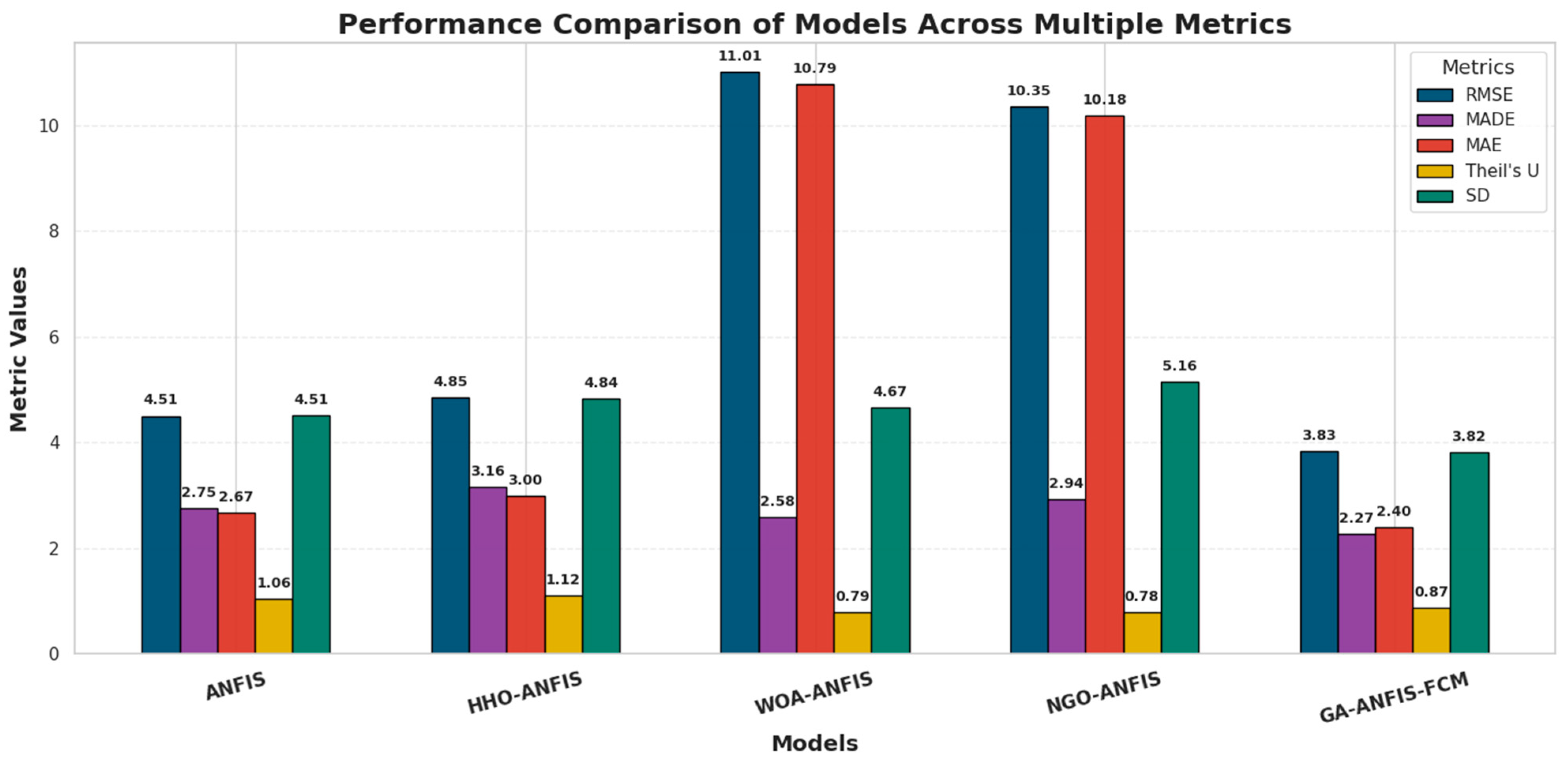
To further reveal the robustness of the GA-ANFIS-FCM4, it was compared with standalone ANFIS and three models using some relatively new generation metaheuristic algorithms. It is noteworthy that both the ANFIS and other hybrid models utilized the same clustering technique, number of clusters, and population size as the GA-ANFIS-FCM4 model to ensure a fair comparative analysis. Harris hawk optimization [61], whale optimization algorithm (WOA) [62], and northern goshawk optimization (NGO) [63] were utilized to optimize the ANFIS structure under the same parameter settings for a fair comparison. The results obtained as seen in Figure 21 show that the optimal model (GA-ANFIS-FCM4) maintained its best performance by having the smallest RMSE, MADE, MAE, and SD, compared to the standalone ANFIS, HHO-ANFIS, WOA-ANFIS, and NGO-ANFIS. A look at the comparison between ANFIS and GA-ANFIS-FCM4 reiterates the need to use intelligent algorithms to optimize ANFIS parameters for stronger predictive performance. By combining intelligent evolutionary algorithms with ANFIS models, an intelligent forecasting system is developed that draws on the adaptive learning of neural networks and the flexible decision making of fuzzy logic to generate better results [64,65].

3.5. Limitations and Future Work

The dataset was anonymized to protect the privacy of the participating schools, which limited our ability to utilize more specific details like detailed structural data, such as individual building sizes and equipment specifications for the model. However, despite these limitations, the dataset remains comprehensive enough to support meaningful analysis of electricity-usage patterns and to identify opportunities for improved energy management. We believe the insights drawn from this study can inform practical interventions and guide future research, particularly in contexts where access to detailed infrastructure data is similarly restricted. Future work could build upon this foundation by exploring correlations between the provided building characteristics and energy-usage trends in more depth. The methodology developed in this study can also serve as a blueprint for similar research initiatives in other regions or with different building types.

4. Conclusions

Ensuring reliable electricity supply in educational institutions requires a robust data-driven approach that accounts for consumption behavior, predictability, and usage patterns. These complexities have led to a shift from traditional forecasting to intelligent machine learning techniques. While some studies have focused on energy prediction in tertiary institutions, little attention has been given to pre-tertiary education settings. In addition, the impacts of clustering techniques and hyperparameter settings have not been explored. In response, this study presented an intelligent hybrid model for predicting electricity consumption, using lower-to-middle-income pre-tertiary education institutions in Western Cape, South Africa, as a case study. Meteorological data such as temperature, relative humidity, windspeed, and wet bulb temperature of the study areas were utilized as the inputs, while electricity-consumption data were used as the output. Two schools were selected from the lower-to-middle-income pre-tertiary as the case study. In total, 70% of the dataset was used for training the developed model and 30% was used for testing and validation. To optimize the structures of ANFIS, two evolutionary algorithms (PSO and GA) were utilized and tested in each of the educational institutions, named Case A and Case B.
Considering the pivotal impact of clustering techniques in machine learning, two renowned clustering techniques along with their key parameters were investigated regarding how they affect electricity prediction. The focus of the study was to identify the best prediction performance among the developed models, specifically in terms of prediction accuracy. This led to the development of numerous sub-models which were analyzed and compared under renowned statistical metrics such as RMSE, MADE, MAE, Theil’s U, and SD. While many of the sub-models deliver good results, the experimental results showed that the GA-ANFIS with four clusters outperformed other hybrid models with the optimal values of RMSE (3.8305), MADE (2.2677), MAE (2.3957), Theil’s U (0.8703), and SD (3.8176), indicating that it had better accuracy and was the model with the least error. Furthermore, the impact of the selection method of GA on hybrid GA-ANFIS was investigated under three other selection methods, Boltzmann, Rank-Based, and Truncation. Our findings showed that Roulette Wheel selection-based GA-ANFIS-FCM (with four clusters) maintained its optimal performance among the three. In addition, the robustness of the optimal model was tested by comparing it with the standalone ANFIS and other hybrid models using new generation metaheuristic algorithms. Results revealed that the optimal model outperformed both the standalone ANFIS and the hybrid models. The highlights of this work are as follows:
  • Energy prediction in pre-tertiary schools is often overlooked. However, understanding their needs is vital to ensure adequate support is provided in order to achieve educational goals, especially in low-to-middle-income settings.
  • Our findings showed that the merger of genetic algorithm, fuzzy c-means clustering technique, and a moderate number of clusters (4) presents an artificial intelligence scheme that can serve as an evidence-based energy-management policies for educational buildings in resource-constrained settings.
  • The choice of selection method in genetic algorithm can impact the performance of GA-based ANFIS models. In addition, the choice of clustering hyperparameters such as number of clusters and clustering radius has a significant impact on the GA-ANFIS models.
  • The application of standalone ANFIS may not offer the most accurate model and it is necessary to optimize its parameters using intelligent evolutionary algorithms.
  • To sum up, this study provides an important insight into the efficacy of the GA-ANFIS-FCM hybrid model in predicting energy consumption in lower-to-middle-income pre-tertiary education institutions. The developed model can contribute helpful insights for policy makers in making informed energy decisions for lower-to-middle-income pre-tertiary education institutions.

Author Contributions

Conceptualization, S.O.O.; Formal analysis, S.O.O.; Funding acquisition, U.B.A. and O.I.O.; Investigation, S.O.O.; Project administration, U.B.A.; Software, S.O.O.; Supervision, U.B.A. and O.I.O.; Validation, S.O.O., U.B.A. and O.I.O.; Visualization, S.O.O.; Writing—original draft, S.O.O.; Writing—review & editing, U.B.A. and O.I.O. All authors have read and agreed to the published version of the manuscript.

Funding

This research received no external funding.

Data Availability Statement

The dataset used in this study is openly available in Mendeley Data at https://doi.org/10.17632/nm2vc4v2br.1, published by Samuels et al. [37], under the Creative Commons Attribution (CC BY 4.0) license.

Acknowledgments

S. O. Oladipo acknowledges Tshwane University of Technology, South Africa, for the support provided for this study.

Conflicts of Interest

The authors declare no conflicts of interest.

Abbreviations

The following abbreviations are used in this manuscript:
ANFISAdaptive neuro-fuzzy inference systems
ANNArtificial neural networks
GPGrid partitioning
SCSubtractive clustering
FCMFuzzy c-means
CRClustering radius
RMSERoot Mean Square Error
SDStandard Deviation
SVMSupport Vector Machine
MAEMean Absolute Error
RCoVCoefficient of Variation
CVRMSECoefficient of Variation of the Root Mean Square Error
MADEMean Absolute Deviation Error
MAPEMean Absolute Percentage Error
MLMachine Learning
FISFuzzy inference systems
MFMembership Function
DTWDynamic Time Warping
LSTMLong short-term memory networks
CNNConvolutional Neural Networks

References

  1. Masebinu, S.O.; Akinlabi, E.T.; Muzenda, E.; Aboyade, A.O. Techno-Economics and Environmental Analysis of Energy Storage for a Student Residence under a South African Time-of-Use Tariff Rate. Energy 2017, 135, 413–429. [Google Scholar] [CrossRef]
  2. Arinaitwe, A.; Aikiriza, F.A.; Kakooza, J.B.; Bagire, V. Sustainable Energy Consumption in African Higher Institutions of Learning: The Nexus of Top Management Commitment and Institutional Pressures. IIMBG J. Sustain. Bus. Innov. 2024, 3, 21–36. [Google Scholar] [CrossRef]
  3. Akpahou, R.; Mensah, L.D.; Quansah, D.A.; Kemausuor, F. Energy Planning and Modeling Tools for Sustainable Development: A Systematic Literature Review. Energy Rep. 2024, 11, 830–845. [Google Scholar] [CrossRef]
  4. Ritchie, H.; Rosado, P.; Roser, M. Energy. Our World in Data; Global Change Data Lab: Oxford, UK, 2023. [Google Scholar]
  5. Jain, S.; Jain, P.K. The Rise of Renewable Energy Implementation in South Africa. Energy Procedia 2017, 143, 721–726. [Google Scholar] [CrossRef]
  6. Ye, Y.; Koch, S.F. Measuring Energy Poverty in South Africa Based on Household Required Energy Consumption. Energy Econ. 2021, 103, 105553. [Google Scholar] [CrossRef]
  7. Adedeji, P.A.; Akinlabi, S.; Ajayi, O.; Madushele, N. Non-Linear Autoregressive Neural Network (NARNET) with SSA Filtering for a University Energy Consumption Forecast. Procedia Manuf. 2019, 33, 176–183. [Google Scholar] [CrossRef]
  8. Ukoba, K.; Olatunji, K.O.; Adeoye, E.; Jen, T.C.; Madyira, D.M. Optimizing Renewable Energy Systems through Artificial Intelligence: Review and Future Prospects. Energy Environ. 2024, 35, 3833–3879. [Google Scholar] [CrossRef]
  9. REN21 RENEWABLES 2017 GLOBAL STATUS REPORT. Available online: https://www.ren21.net/gsr-2017/ (accessed on 12 June 2025).
  10. Adedeji, P.; Madushele, N.; Akinlabi, S. Adaptive Neuro-Fuzzy Inference System (ANFIS) for a Multi-Campus Institution Energy Consumption Forecast in South Africa. In Proceedings of the International Conference on Industrial Engineering and Operations Management, Washington, DC, USA, 27–29 September 2018; pp. 950–958. [Google Scholar]
  11. Department of Energy. A Survey of Energy Related Behaviour and Perceptions in South Africa; Government Printer: Mumbai, Maharashtra, 2013. [Google Scholar]
  12. Minelli, F.; Ciriello, I.; Minichiello, F.; D’Agostino, D. From Net Zero Energy Buildings to an Energy Sharing Model—The Role of NZEBs in Renewable Energy Communities. Renew Energy 2024, 223, 120110. [Google Scholar] [CrossRef]
  13. Ragupathi, C.; Dhanasekaran, S.; Vijayalakshmi, N.; Salau, A.O. Prediction of Electricity Consumption Using an Innovative Deep Energy Predictor Model for Enhanced Accuracy and Efficiency. Energy Rep. 2024, 12, 5320–5337. [Google Scholar] [CrossRef]
  14. van der Meer, D.W.; Shepero, M.; Svensson, A.; Widén, J.; Munkhammar, J. Probabilistic Forecasting of Electricity Consumption, Photovoltaic Power Generation and Net Demand of an Individual Building Using Gaussian Processes. Appl. Energy 2018, 213, 195–207. [Google Scholar] [CrossRef]
  15. Kim, H.; Park, S.; Kim, S. Time-Series Clustering and Forecasting Household Electricity Demand Using Smart Meter Data. Energy Rep. 2023, 9, 4111–4121. [Google Scholar] [CrossRef]
  16. Ramos, D.; Faria, P.; Morais, A.; Vale, Z. Using Decision Tree to Select Forecasting Algorithms in Distinct Electricity Consumption Context of an Office Building. Energy Rep. 2022, 8, 417–422. [Google Scholar] [CrossRef]
  17. Yang, H.; Ran, M.; Zhuang, C. Prediction of Building Electricity Consumption Based on Joinpoint−Multiple Linear Regression. Energies 2022, 15, 8543. [Google Scholar] [CrossRef]
  18. Shijer, S.S.; Jassim, A.H.; Al-Haddad, L.A.; Abbas, T.T. Evaluating Electrical Power Yield of Photovoltaic Solar Cells with K-Nearest Neighbors: A Machine Learning Statistical Analysis Approach. E-Prime Adv. Electr. Eng. Electron. Energy 2024, 9, 100674. [Google Scholar] [CrossRef]
  19. Jónsson, T.; Pinson, P.; Nielsen, H.A.; Madsen, H. Exponential Smoothing Approaches for Prediction in Real-Time Electricity Markets. Energies 2014, 7, 3710–3732. [Google Scholar] [CrossRef]
  20. Mi, J.; Fan, L.; Duan, X.; Qiu, Y. Short-Term Power Load Forecasting Method Based on Improved Exponential Smoothing Grey Model. Math. Probl. Eng. 2018, 2018, 3894723. [Google Scholar] [CrossRef]
  21. Deb, C.; Zhang, F.; Yang, J.; Lee, S.E.; Shah, K.W. A Review on Time Series Forecasting Techniques for Building Energy Consumption. Renew. Sustain. Energy Rev. 2017, 74, 902–924. [Google Scholar] [CrossRef]
  22. Tarmanini, C.; Sarma, N.; Gezegin, C.; Ozgonenel, O. Short Term Load Forecasting Based on ARIMA and ANN Approaches. Energy Rep. 2023, 9, 550–557. [Google Scholar] [CrossRef]
  23. Mohammed, N.A.; Al-Bazi, A. An Adaptive Backpropagation Algorithm for Long-Term Electricity Load Forecasting. Neural Comput. Appl. 2021, 34, 477. [Google Scholar] [CrossRef]
  24. Elbeltagi, E.; Wefki, H. Predicting Energy Consumption for Residential Buildings Using ANN through Parametric Modeling. Energy Rep. 2021, 7, 2534–2545. [Google Scholar] [CrossRef]
  25. Oladipo, S.O.; Sun, Y.; Amole, A.O. Analysis of the Impact of Clustering Techniques and Parameters on Evolutionary-Based Hybrid Models for Forecasting Electricity Consumption. IEEE Access 2023, 11, 82838–82856. [Google Scholar] [CrossRef]
  26. Jang, J.S.R. ANFIS: Adaptive-Network-Based Fuzzy Inference System. IEEE Trans. Syst. Man Cybern. 1993, 23, 665–685. [Google Scholar] [CrossRef]
  27. Ani, K.A.; Agu, C.M. Predictive Comparison and Assessment of ANFIS and ANN, as Efficient Tools in Modeling Degradation of Total Petroleum Hydrocarbon (TPH). Clean. Waste Syst. 2022, 3, 100052. [Google Scholar] [CrossRef]
  28. Ghenai, C.; Al-Mufti, O.A.A.; Al-Isawi, O.A.M.; Amirah, L.H.L.; Merabet, A. Short-Term Building Electrical Load Forecasting Using Adaptive Neuro-Fuzzy Inference System (ANFIS). J. Build. Eng. 2022, 52, 104323. [Google Scholar] [CrossRef]
  29. Bilgili, M.; Yildirim, A.; Ozbek, A.; Celebi, K.; Ekinci, F. Long Short-Term Memory (LSTM) Neural Network and Adaptive Neuro-Fuzzy Inference System (ANFIS) Approach in Modeling Renewable Electricity Generation Forecasting. Int. J. Green Energy 2021, 18, 578–594. [Google Scholar] [CrossRef]
  30. Rathor, R.D.; Bharagava, A. Day Ahead Regional Electrical Load Forecasting Using ANFIS Techniques. J. Inst. Eng. Ser. B 2020, 101, 475–495. [Google Scholar] [CrossRef]
  31. Chévez, P.; Martini, I. Applying Neural Networks for Short and Long-Term Hourly Electricity Consumption Forecasting in Universities: A Simultaneous Approach for Energy Management. J. Build. Eng. 2024, 97, 110612. [Google Scholar] [CrossRef]
  32. Begić Juričić, H.; Krstić, H. Comparing MLR and ANN Models for School Building Electrical Energy Prediction in Osijek-Baranja County in Croatia. Energy Rep. 2024, 12, 3595–3606. [Google Scholar] [CrossRef]
  33. Stošović, M.A.; Radivojević, N.; Ivanova, M. Electricity Consumption Prediction in an Electronic System Using Artificial Neural Networks. Electronics 2022, 11, 3506. [Google Scholar] [CrossRef]
  34. Al-Qaness, M.A.A.; Elaziz, M.A.; Ewees, A.A. Oil Consumption Forecasting Using Optimized Adaptive Neuro-Fuzzy Inference System Based on Sine Cosine Algorithm. IEEE Access 2018, 6, 68394–68402. [Google Scholar] [CrossRef]
  35. Naik, M.; Abiodun, B.J. Modelling the Potential of Land Use Change to Mitigate the Impacts of Climate Change on Future Drought in the Western Cape, South Africa. Theor. Appl. Climatol. 2024, 155, 6371–6392. [Google Scholar] [CrossRef]
  36. Botai, C.M.; Botai, J.O.; De Wit, J.P.; Ncongwane, K.P.; Adeola, A.M. Drought Characteristics over the Western Cape Province, South Africa. Water 2017, 9, 876. [Google Scholar] [CrossRef]
  37. Samuels, J.A.; Michael-Ahile, T.; Booysen, M.J. (Thinus) Dataset on Electricity Usage Measurement for Lower-to-Middle-Income Primary and Secondary Schools in Western Cape, South Africa. Data Brief 2025, 59, 111321. [Google Scholar] [CrossRef]
  38. Rahman, M.S.; Ali, M.H. Adaptive Neuro Fuzzy Inference System (ANFIS)-Based Control for Solving the Misalignment Problem in Vehicle-to-Vehicle Dynamic Wireless Charging Systems. Electronics 2025, 14, 507. [Google Scholar] [CrossRef]
  39. Kamarian, S.; Yas, M.H.; Pourasghar, A.; Daghagh, M. Application of Firefly Algorithm and ANFIS for Optimisation of Functionally Graded Beams. J. Exp. Theor. Artif. Intell. 2014, 26, 197–209. [Google Scholar] [CrossRef]
  40. Petković, D.; Ćojbašić, Ž.; Nikolić, V.; Shamshirband, S.; Mat Kiah, M.L.; Anuar, N.B.; Abdul Wahab, A.W. Adaptive Neuro-Fuzzy Maximal Power Extraction of Wind Turbine with Continuously Variable Transmission. Energy 2014, 64, 868–874. [Google Scholar] [CrossRef]
  41. Jayaprabha, M.; Felcy, P. A Review of Clustering, Its Types and Techniques. Int. J. Innov. Sci. Res. Technol. 2018, 3, 127–130. [Google Scholar]
  42. Chiu, S.L. Fuzzy Model Identification Based on Cluster Estimation. J. Intell. Fuzzy Syst. 1994, 2, 267–278. [Google Scholar] [CrossRef]
  43. Sayeed, M.S.; Hossen, M.J.; Rahman, A.; Samsuddin, K.; Rokhani, F. A Modified Hybrid Fuzzy Clustering Algorithm for Data Partitions. Aust. J. Basic Appl. Sci. 2011, 5, 674–681. [Google Scholar]
  44. Deb, A.K. Introduction to Soft Computing Techniques: Artificial Neural Networks, Fuzzy Logic and Genetic Algorithms. Soft Comput. Text. Eng. 2011, 3–24. [Google Scholar] [CrossRef]
  45. Holland, J.H. Genetic Algorithms. Sci. Am. 1992, 267, 66–73. [Google Scholar] [CrossRef]
  46. Kennedy, R.E.J. Particle Swarm Optimization. In Proceedings of the ICNN’95—International Conference on Neural Networks, Perth, WA, Australia, 27 November–1 December 1995; pp. 1942–1948. [Google Scholar]
  47. Hossain, M.; Mekhilef, S.; Afifi, F.; Halabi, L.M.; Olatomiwa, L.; Seyedmahmoudian, M.; Horan, B.; Stojcevski, A. Application of the Hybrid ANFIS Models for Long Term Wind Power Density Prediction with Extrapolation Capability. PLoS ONE 2018, 13, e0193772. [Google Scholar] [CrossRef] [PubMed]
  48. Olatunji, K.O.; Adeleke, O.; Jen, T.-C.; Madyira, D.M. Impact of Acidic Pretreatment on Biomethane Yield from Xyris Capensis: Experimental and In-Depth Data-Driven Insight. Processes 2025, 13, 1997. [Google Scholar] [CrossRef]
  49. Rajabi, A.; Eskandari, M.; Ghadi, M.J.; Li, L.; Zhang, J.; Siano, P. A Comparative Study of Clustering Techniques for Electrical Load Pattern Segmentation. Renew. Sustain. Energy Rev. 2020, 120, 109628. [Google Scholar] [CrossRef]
  50. Sharma, N.; Katyal, R. Investigation on Combined Impacts of Different Clustering Techniques and Enhanced K-Means Algorithm. Commun. Comput. Inf. Sci. 2025, 2238 CCIS, 251–260. [Google Scholar] [CrossRef]
  51. Mitchell, M. An Introduction to Genetic Algorithms; The MIT Press: Cambridge, MA, USA, 1998. [Google Scholar]
  52. Mills, K.L.; Filliben, J.J.; Haines, A.L. Determining Relative Importance and Effective Settings for Genetic Algorithm Control Parameters. Evol. Comput. 2015, 23, 309–342. [Google Scholar] [CrossRef]
  53. Ghahramani, M.; Shiri, N. An Adaptive Neuro-Fuzzy Inference System Optimized by Genetic Algorithm for Brain Tumour Detection in Magnetic Resonance Images. IET Image Process 2024, 18, 1358–1372. [Google Scholar] [CrossRef]
  54. Savrun, M.M.; İnci, M. Adaptive Neuro-Fuzzy Inference System Combined with Genetic Algorithm to Improve Power Extraction Capability in Fuel Cell Applications. J. Clean Prod. 2021, 299, 126944. [Google Scholar] [CrossRef]
  55. Arana-Jimenez, M.; Dogan, O.; Avvad, H. Fuzzy Clustering Based on Activity Sequence and Cycle Time in Process Mining. Axioms 2025, 14, 351. [Google Scholar] [CrossRef]
  56. Thong, P.H.; Canh, H.T.; Lan, L.T.H.; Huy, N.T.; Giang, N.L. Multi-View Picture Fuzzy Clustering: A Novel Method for Partitioning Multi-View Relational Data. Comput. Mater. Contin. 2025, 83, 5461–5485. [Google Scholar] [CrossRef]
  57. Onakpojeruo, E.P.; Uzun, B.; David, L.R.; Ozsahin, I.; Ozsahin, D.U. Selection Techniques in Genetic Algorithm. In Proceedings of the International Conference on Developments in eSystems Engineering, DeSE, Khorfakkan, UK, 6–8 November 2024; pp. 411–416. [Google Scholar] [CrossRef]
  58. Nemati, K.; Refahi Sheikhani, A.H.; Kordrostami, S.; Khoshhal Roudposhti, K. New Hybrid Feature Selection Approaches Based on ANN and Novel Sparsity Norm. J. Electr. Comput. Eng. 2024, 2024, 7112770. [Google Scholar] [CrossRef]
  59. Haq, E.U.; Ahmad, I.; Hussain, A.; Almanjahie, I.M. A Novel Selection Approach for Genetic Algorithms for Global Optimization of Multimodal Continuous Functions. Comput. Intell. Neurosci. 2019, 2019, 8640218. [Google Scholar] [CrossRef]
  60. Goldberg, D.E.; Deb, K. A Comparative Analysis of Selection Schemes Used in Genetic Algorithms. Found. Genet. Algorithms 1991, 1, 69–93. [Google Scholar] [CrossRef]
  61. Heidari, A.A.; Mirjalili, S.; Faris, H.; Aljarah, I.; Mafarja, M.; Chen, H. Harris Hawks Optimization: Algorithm and Applications. Future Gener. Comput. Syst. 2019, 97, 849–872. [Google Scholar] [CrossRef]
  62. Mirjalili, S.; Lewis, A. The Whale Optimization Algorithm. Adv. Eng. Softw. 2016, 95, 51–67. [Google Scholar] [CrossRef]
  63. Dehghani, M.; Hubálovský, Š.; Trojovský, P. Northern Goshawk Optimization: A New Swarm-Based Algorithm for Solving Optimization Problems. IEEE Access 2021, 9, 162059–162080. [Google Scholar] [CrossRef]
  64. Karaboga, D.; Kaya, E. Adaptive Network Based Fuzzy Inference System (ANFIS) Training Approaches: A Comprehensive Survey. Artif. Intell. Rev. 2018, 52, 2263–2293. [Google Scholar] [CrossRef]
  65. Ghordoyee Milan, S.; Roozbahani, A.; Arya Azar, N.; Javadi, S. Development of Adaptive Neuro Fuzzy Inference System –Evolutionary Algorithms Hybrid Models (ANFIS-EA) for Prediction of Optimal Groundwater Exploitation. J. Hydrol. 2021, 598, 126258. [Google Scholar] [CrossRef]
Figure 1. Integrated renewable energy system for smart energy management in educational buildings.
Mathematics 13 02648 g001
Figure 2. Categorization of machine learning methods.
Mathematics 13 02648 g002
Figure 3. Architectural flow of hybrid models.
Mathematics 13 02648 g003
Figure 4. ANFIS model architecture.
Mathematics 13 02648 g004
Figure 5. Proposed GA-ANFIS model.
Mathematics 13 02648 g005
Figure 6. Proposed PSO-ANFIS model.
Mathematics 13 02648 g006
Figure 7. Performance evaluation of the GA-ANFIS-SC model with varying clustering radii for Case A.
Mathematics 13 02648 g007
Figure 8. Performance evaluation of the GA-ANFIS-FCM model with varying clustering numbers for Case A.
Mathematics 13 02648 g008
Figure 9. Performance evaluation of the PSO-ANFIS-SC model with varying clustering radii for Case A.
Mathematics 13 02648 g009
Figure 10. Performance evaluation of the PSO-ANFIS-FCM model with varying clustering numbers for Case A.
Mathematics 13 02648 g010
Figure 11. Performance evaluation of the GA-ANFIS-SC model with varying clustering radii for Case B.
Mathematics 13 02648 g011
Figure 12. Performance evaluation of the GA-ANFIS-FCM model with varying number of clusters for Case B.
Mathematics 13 02648 g012
Figure 13. Performance evaluation of the PSO-ANFIS-SC model with varying number of clusters for Case B.
Mathematics 13 02648 g013
Figure 14. Performance evaluation of the PSO-ANFIS-FCM model with varying number of clusters.
Mathematics 13 02648 g014
Figure 15. Radar plots for sub-optimal models for Case A.
Mathematics 13 02648 g015
Figure 16. Optimal GA-ANFIS-SC with cluster radius of 0.4.
Mathematics 13 02648 g016
Figure 17. Radar plots for sub-optimal models for Case B.
Mathematics 13 02648 g017
Figure 18. Optimal GA-ANFIS-FCM with four clusters.
Mathematics 13 02648 g018
Figure 19. Comparison between the two best models in Cases A and B.
Mathematics 13 02648 g019
Figure 20. Comparison between different selection methods for GA-ANFIS-FCM.
Mathematics 13 02648 g020
Figure 21. Comparative evaluation of model performance between standalone ANFIS and hybrid models.
Mathematics 13 02648 g021
Table 1. Summary of the contributions of previous studies.
ReferenceModel/Machine Learning UsedWork Performed/ContributionsArea of Application
Meer et al. [14]Gaussian Processes (GPs)Utilized GPs for probabilistic forecasting of residential electricity consumption.Residential building
Kim et al. [15]Various (ARIMA, DSHW, TBATS, NNAR, NARX)Forecasted household electricity demand using time-series clustering.Residential
Ramos et al. [16]ANN, k-NN, decision treesUsed decision trees to select forecasting algorithms for an office building.Office building
Tarmanini et al. [22]ARIMA, ANNCompared ARIMA and ANN for short-term load forecasting.Residential
Mohammed et al. [23]ANN, Adaptive Backpropagation Algorithm (ABPA)Developed an improved ANN with an adaptive algorithm for long-term load forecasting.General
Elbeltagi et al. [24]ANNPresented an ANN-based methodology to predict residential building energy usage.Residential building
Ghenai et al. [28]Adaptive Neuro-Fuzzy Inference System (ANFIS)Developed an ANFIS model for very short-term energy-consumption forecasts.Educational building
Bilgili et al. [29]LSTM, ANFISApplied LSTM and ANFIS to forecast renewable electricity generation.Renewable energy generation
Rathor et al. [30]ANFISDeveloped ANFIS models for day-ahead regional electrical load forecasting.Regional
Pedro et al. [31]Neural NetworksDeveloped simultaneous short-term and long-term electricity-forecasting models for a university.University building
Ana et al. [32]ANN, Multiple Linear Regression (MLR)Compared ANN and MLR models for predicting school building energy consumption.School building
Miona et al. [33]RNN, LSTM, GRUProposed a method for electricity-consumption prediction using various recurrent neural networks.Cold storage facility
Present StudyHybrid ANFIS models: optimized with GA and PSO utilized with Subtractive Clustering (SC) and Fuzzy C-Means (FCM)Developed hybrid evolutionary-based ANFIS models for electricity forecasting, investigating the impact of clustering and hyperparameters.Lower-to-middle-income pre-tertiary schools in Western Cape, South Africa
Table 2. Socio-economic and educational characteristics of case study schools.
QuintileCaseLearnersSchool TypeEducators
1Case A1405Primary43
2Case B1159Combined29
Table 3. Parameter settings for the model.
ParametersNamesValues
SCCluster radius (CR)3–7
FCMMinimum improvement0.3–0.6
Number of exponents for partitioning matrix1 × 10−5
Number of clusters2
General settings of the hybrid models Maximum   iteration   ( t m a x ) 100
Population size100
Number of inputs4
Number of outputs1
GA Crossover   probability   ( P c ) 0.40
Mutation   probability   ( P m ) 0.15
Selection mechanismRoulette wheel
PSO Cognitive   coefficient   ( c 1 ) 2
Social   coefficient   ( c 2 ) 2
Inertia   weight   damping   ratio   ( ω d a m p ) 0.99
Inertia   weight   ( ω ) 1
Table 4. Performance evaluation of GA-ANFIS-SC model for Case A.
Clustering RadiusRMSEMADEMAETheil’s USD
GA-ANFIS-SC0.36.12073.70703.72770.87646.1333
0.45.36403.19173.23960.80355.3641
0.56.16263.75383.85200.92996.1588
0.66.15723.52793.60180.98346.1649
0.76.07273.62453.76180.90936.0611
Table 5. Performance evaluation of GA-ANFIS-FCM model for Case A.
No. of ClustersRMSEMADEMAETheil’s USD
GA-ANFIS-FCM26.57634.32444.23071.13536.5782
36.13973.85153.73141.14026.1375
45.87773.81173.84661.00975.8886
56.44334.13554.01811.12486.4486
66.30444.11474.09451.05046.3181
77.15384.56934.24971.25257.1165
Table 6. Performance evaluation of PSO-ANFIS-SC model for Case A.
Clustering RadiusRMSEMADEMAEUSD
PSO-ANFIS-SC0.36.48853.98083.93340.90776.5002
0.46.19183.73913.52850.98286.1478
0.56.29323.66413.64660.93586.3071
0.66.75664.32263.96311.18916.7125
0.76.35014.02634.08050.95086.3352
Table 7. Performance evaluation of PSO-ANFIS-FCM model for Case A.
No. of ClustersRMSEMADEMAETheil’s USD
PSO-ANFIS-FCM26.10743.90963.89301.05966.1209
36.10924.00394.03351.01116.1219
45.94573.97384.19330.93905.9108
56.71274.23904.00631.20106.6951
66.60954.36824.33981.08006.6236
Table 8. Performance evaluation of GA-ANFIS-SC for Case B.
Clustering RadiusRMSEMADEMAETheil’s USD
GA-ANFIS-SC0.34.24322.53852.53730.84664.2527
0.44.28572.53412.57330.85684.2807
0.54.19682.48382.53850.90454.2024
0.64.00902.39662.47910.91104.0087
0.74.77082.87862.81061.07134.7792
Table 9. Performance evaluation of GA-ANFIS-FCM for Case B.
No. of ClustersRMSEMADEMAETheil’s USD
GA-ANFIS-FCM24.28092.66772.66970.97524.2905
35.19833.27163.04801.22165.1909
43.83052.26772.39570.87033.8176
54.25832.58122.55581.00194.2667
64.96992.95902.77651.16234.9625
Table 10. Performance evaluation of PSO-ANFIS-SC for Case B.
Clustering RadiusRMSEMADEMAETheil’s USD
PSO-ANFIS-SC0.34.43442.54622.55460.93194.4443
0.44.80022.89502.79621.02864.7937
0.54.27612.59972.44570.99154.2591
0.64.27732.41022.41230.92724.2869
0.74.75092.77192.66551.04224.7538
Table 11. Performance evaluation of PSO-ANFIS-FCM for Case B.
Number of ClustersRMSEMADEMAETheil’s USD
PSO-ANFIS-FCM24.20022.49282.64750.91944.1853
34.19142.51252.60420.96984.1918
44.82352.99793.01100.99474.8340
54.45952.72262.70931.03284.4695
64.28672.64642.72060.96164.2891
Table 12. Comparison between optimal sub-models in Case A.
Model RMSEMADEMAETheil’s USD
GA-ANFIS-SCCluster radius: 0.45.36403.19173.23960.80355.3641
GA-ANFIS-FCMNumber of clusters: 45.87773.81173.84661.00975.8886
PSO-ANFIS-SCCluster radius: 0.46.19183.73913.52850.98286.1478
PSO-ANFIS-FCMNumber of clusters: 45.94573.97384.19330.93905.9108
Table 13. Comparison between optimal sub-models in Case B.
Model RMSEMADEMAETheil’s USD
GA-ANFIS-SCClustering radius: 0.64.00902.39662.47910.91104.0087
GA-ANFIS-FCMNumber of clusters: 43.83052.26772.39570.87033.8176
PSO-ANFIS-SCClustering radius: 0.64.27732.41022.41230.92724.2869
PSO-ANFIS-FCMNumber of clusters: 24.20022.49282.64750.91944.1853
Disclaimer/Publisher’s Note: The statements, opinions and data contained in all publications are solely those of the individual author(s) and contributor(s) and not of MDPI and/or the editor(s). MDPI and/or the editor(s) disclaim responsibility for any injury to people or property resulting from any ideas, methods, instructions or products referred to in the content.