An Adaptive Projection Differential Dynamic Programming Method for Control Constrained Trajectory Optimization

Abstract

To address the issue of missing constraints on control variables in the trajectory optimization problem of the differential dynamic programming (DDP) method, the adaptive projection differential dynamic programming (AP-DDP) method is proposed. The core of the AP-DDP method is to introduce adaptive relaxation coefficients to dynamically adjust the smoothness of the projection function and to effectively solve the gradient disappearance problem that may occur when the control variable is close to the constraint boundary. Additionally, the iterative strategy of the relaxation coefficient accelerates the search for a feasible solution in the initial stage, thereby improving the algorithm’s efficiency. When applied to three trajectory optimization problems, compared with similar truncated DDP, projected DDP, and Box-DDP methods, the AP-DDP method found the optimal solution in the shortest computation time, thereby proving the efficiency of the proposed algorithm. While ensuring the iterative process reaches the global optimum, the computing time of the AP-DDP method was reduced by 32.8%, 13.3%, and 18.5%, respectively, in the three examples.

1. Introduction

Trajectory optimization is a vital technology for solving optimal control problems, holding significant theoretical research importance and engineering application value [1,2]. The trajectory optimization problem is a type of multi-stage, nonlinear optimal control challenge with fixed objective states, control variables, and path constraints. Numerical methods to solve these problems are mainly divided into indirect and direct approaches [3]. Indirect methods include Pontryagin’s principle of extreme value [4] and the variational method [5], which derive control strategies by constructing the accompanying equations and applying optimality conditions. Their strengths lie in their theoretical rigor and ability to precisely satisfy optimality conditions. For instance, the literature [6] has used the variational method to derive dynamic optimality control conditions for rocket flight parameters. However, indirect methods involve complex accompanying equations, which require intricate mathematical derivations, limiting their practical application in engineering. Conversely, direct methods, such as targeting [7] and pseudospectral methods [8], convert continuous optimal control problems into nonlinear planning problems through discretization, which are then solved using optimization algorithms, like sequential quadratic programming (SQP) [9,10]. Direct methods are favored for their ease of implementation and adaptability to complex constraints, making them more prevalent in industry and engineering practice. For example, the literature [11,12] has explored the use of the Gauss pseudospectral method in local orbit optimization for deep space exploration with small-thrust rockets and in trajectory optimization during the climb phase of a hybrid-power aircraft. The literature [13] has employed the targeting method to optimize the trajectory of a second-stage rocket and the recovery process for the first stage. Recently, machine learning approaches have introduced new ideas for solving optimal control problems. Reinforcement learning (RL) [14], for example, can handle optimal control in both model-free and model-based scenarios, making it suitable for complex, high-dimensional, nonlinear control tasks. Model predictive control (MPC) [15] is a model-based optimal control strategy for roll optimization, with the literature [16] demonstrating its use for trajectory optimization during a rocket’s vertical landing phase. When an accurate system model is available, MPC is characterized by high computational efficiency.

The differential dynamic programming (DDP) method [17,18] has significantly improved robot trajectory optimization in recent years. DDP breaks down the global optimization problem into multiple local optimization problems over time. Its use of backward propagation and second-order approximate dynamic updates of the control strategy helps avoid the high-dimensional computational burden of SQP when handling the full-variable Hessian matrix. Additionally, it overcomes the numerical stability issues of variational methods in solving two-point boundary value problems. It offers high computational efficiency for nonlinear system optimal control problems [19]. However, the iterative process of the DDP method does not consider control variable constraints. This leads to challenges in trajectory optimization tasks that involve control variable constraints. As a result, researchers have introduced various improvement strategies, including penalty function methods [20], augmented Lagrangian methods [21], truncated DDP methods [22], and projected DDP methods [23]. Among these, the penalty function method is a soft-constraint approach that incorporates penalty terms into the loss function to manage constraints, with the advantage of straightforward implementation. For example, Howell et al. [21] transformed the constrained optimization problem into an unconstrained problem by adding penalty terms and Lagrange multipliers into the objective function, thus integrating constraints within the DDP framework. However, since the penalty function method is a soft-constraint technique, it may still cause the control variables to exceed their allowable range. The truncated DDP method [22] offers a direct approach to constraint handling: control variables are forcibly truncated to the boundary values if they surpass the specified limits. Nonetheless, this method can introduce issues with gradient discontinuity at the boundaries, potentially resulting in unstable optimization or complicated convergence. The projected DDP method [23] mitigates this by mapping control variables into the constraint range via projection functions, which provides better smoothness at the boundaries than the truncated approach. However, gradient vanishing remains problematic as control variables approach the boundaries.

Compared to truncated methods, the projected method provides the advantage of smooth gradient variations in control variables. It prevents the issue of gradient discontinuity during the iterative process. However, the projected DDP method might struggle to reach the boundaries of control variables during iteration, and the cost function can fluctuate slightly between iterations, possibly leading to premature convergence and causing the algorithm to get stuck in a local optimum. Box-DDP is a box-constraint method specifically designed for control variables; unlike the previous two methods, which adjust control ranges during backward propagation, it directly accounts for control restrictions at each time step. It incorporates the box constraints of control variables into the quadratic programming sub-problem for solution. When minimizing the quadratic approximation of the action value function, the constraint condition is the box constraint of the control variables. Nonetheless, the Box-DDP method requires solving a quadratic programming sub-problem at each time step, which increases complexity and decreases computational efficiency.

Researchers have suggested several ways to improve further the performance of the DDP method in dealing with constraint problems. For example, Cao et al. [18] converted the polynomial trajectory generation problem into an optimal control problem in a state space form. They guaranteed the safety and feasibility of the trajectory by adding control points and dynamic feasibility constraints. Finally, they used dynamic programming to solve the constrained optimal control problem. Xie et al. [19] introduced the constrained differential dynamic programming method, developed the recursive quadratic approximation formula with nonlinear constraints, and identified a set of active constraints at each time step, enabling the practical addition of control constraints. Aoyama et al. [24] further enhanced the DDP method’s ability to handle nonlinear constraint problems by combining slack variables with augmented Lagrangian techniques. In summary, the projection DDP method effectively limits the control variables to a fixed range through the projection function. However, gradient disappearance may occur when the control variables are near the constraint boundary, which can cause the algorithm to get stuck in a local optimum.

To address the above issues, this paper improves the existing projection function and introduces an adaptive projection differential dynamic programming (AP-DDP) method. The main innovation of this approach is the addition of an adaptive relaxation coefficient to dynamically adjust the smoothness of the projection function, effectively preventing the gradient disappearance that can occur when control variables are near the constraint boundary, which can cause the algorithm to get stuck in a local optimum. The iterative relaxation coefficient also helps accelerate the search for feasible solutions in the early stage, increasing the algorithm’s efficiency. The structure of this paper is as follows: Section 2 explains the principle of the DDP method; Section 3 details the AP-DDP method proposed here; Section 4 applies this method to three trajectory optimization examples, generating optimal trajectories and comparing them with other similar methods; Section 5 summarizes the research results and discusses future prospects.

2. Related Technology

DDP is an optimal control algorithm for trajectory optimization. It uses local quadratic approximation for dynamic processes and cost functions. Compared to the SQP and the variational method, it has notable advantages in memory efficiency and solution speed. Consider a model with discrete-time dynamics, which is calculated as follows:

$$x_{i+1}=f(x_i,u_i)$$

(1)

where $u_i\in {\mathrm{R}}^m$ represents the control vector. The state sequence $\left[x_1,x_2,\cdots ,x_n\right]$ is generated by the initial state $x_0$ and the control sequence $\left[u_0,u_1,\cdots ,u_{n-1}\right]$. The total cost is the sum of running cost and final cost, which is calculated as follows:

$$J=l_f(x_N)+{\displaystyle {\sum }_{k=0}^{N-1}{l}_k(x_k,u_k)}$$

(2)

where $l_f(x_N)$ represents the final cost and $l_k(x_k,u_k)$ represents the running cost. The optimization objective is to solve for the optimal control sequence $U$ to minimize the total cost $J$, as follows:

$$U^{*}=\underset{U}{\arg \min } J(x_0,U)$$

(3)

where $U^{*}$ represents the optimal control sequence. The DDP algorithm iteratively optimizes the control sequence through backward pass and forward pass, gradually reducing the total cost until convergence. The backward pass starts from the final time and goes back to the initial time, updating progressively the value function, which is calculated as follows:

$${\mathrm{V}}_i(x_i)=\underset{u_i}{\min }[l(x_i,u_i)+{\mathrm{V}}_{i+1}(f(x_i,u_i))]$$

(4)

where V represents the minimum cost at time $i$. According to Bellman’s principle, the sub-strategy of the global optimal policy is also the optimal solution. To further analyze the optimal control problem, the action value function $\mathrm{Q}$ is introduced to explore the impact of control inputs on the value function. Its definition is calculated as follows:

$$\mathrm{Q}\left(\delta x_k,\delta u_k\right)\approx {\displaystyle \frac{1}{2}}{\left[\begin{array}{c}1\\ \delta x_k\\ \delta u_k\end{array}\right]}^T\left[\begin{array}{ccc}0& {\mathrm{Q}}_x^T& {\mathrm{Q}}_u^T\\ {\mathrm{Q}}_x& {\mathrm{Q}}_{xx}& {\mathrm{Q}}_{ux}^T\\ {\mathrm{Q}}_u& {\mathrm{Q}}_{ux}& {\mathrm{Q}}_{uu}\end{array}\right]\left[\begin{array}{c}1\\ \delta x_k\\ \delta u_k\end{array}\right]$$

(5)

The derivatives part can be expanded as follows:

$$\begin{array}{l}{\mathrm{Q}}_x=l_x+f_x^T{\mathrm{V}}_x\hfill \\ {\mathrm{Q}}_u=l_u+f_u^T{\mathrm{V}}_x\hfill \\ {\mathrm{Q}}_{xx}=l_{xx}+f_x^T{\mathrm{V}}_{xx}{f}_x+{\mathrm{V}}_x{f}_{xx}\hfill \\ {\mathrm{Q}}_{uu}=l_{uu}+f_u^T{\mathrm{V}}_{xx}{f}_u+{\mathrm{V}}_x{f}_{uu}\hfill \\ {\mathrm{Q}}_{ux}=l_{ux}+f_u^T{\mathrm{V}}_{xx}{f}_x+{\mathrm{V}}_x{f}_{ux}\hfill \end{array}$$

(6)

where ${\mathrm{V}}_x$ represents the gradient of the value function, and ${\mathrm{V}}_{xx}$ represents the Hessian matrix of the value function. By minimizing the action value function, the control variation can be obtained as follows:

$$\delta u_k=\arg \min Q\left(\delta x_k,\delta u_k\right)=-{\mathrm{Q}}_{uu}^{-1}{\mathrm{Q}}_{ux}\delta x-{\mathrm{Q}}_{uu}^{-1}{\mathrm{Q}}_u$$

(7)

Then, the value function is backtracked to update its gradient and the Hessian matrix at the current time, as follows:

$$\begin{array}{l}{\mathrm{V}}_x={\mathrm{Q}}_x-{\mathrm{Q}}_{xu}{\mathrm{Q}}_{uu}^{-1}{\mathrm{Q}}_u\hfill \\ {\mathrm{V}}_{xx}={\mathrm{Q}}_{xx}-{\mathrm{Q}}_{xu}{\mathrm{Q}}_{uu}^{-1}{\mathrm{Q}}_{ux}\hfill \end{array}$$

(8)

After the backward pass is completed, the forward pass begins. Starting from the initial state, the control and state are gradually updated to generate new trajectories, as follows:

$$\begin{array}{l}{u}_t^{new}=u_t-{\mathrm{Q}}_{uu}^{-1}{\mathrm{Q}}_{ux}(x_t^{new}-x_t)-{\mathrm{Q}}_{uu}^{-1}{\mathrm{Q}}_u\hfill \\ x_{t+1}^{new}=f(x_t^{new},u_t^{new})\hfill \end{array}$$

(9)

In the above DDP algorithm iteration process, the constraints of the control variables were not considered, which led to the algorithm’s limitations when solving the optimal control problem with constraints.

The way to add control constraints in DDP usually involves using truncation or projection methods to limit the control trajectory within a specified range. For example, the BOX-DDP method calculates a series of quadratic programming problems in each iteration, which results in low computational efficiency. The truncation DDP method has the problem of discontinuous gradient changes at the constraint boundaries, making it difficult to converge to the optimal solution. The DDP method has the issue that the gradient information becomes extremely small at the contact boundaries, which hinders the formation of an effective direction for updating the gradient, thereby leading to getting trapped in a local optimal solution trap.

3. Adaptive Projection Differential Dynamic Programming

To address the shortcomings of the projected DDP, this section presents the proposed adaptive projection differential dynamic programming (AP-DDP) method and the search strategy.

3.1. The Framework of AP-DDP

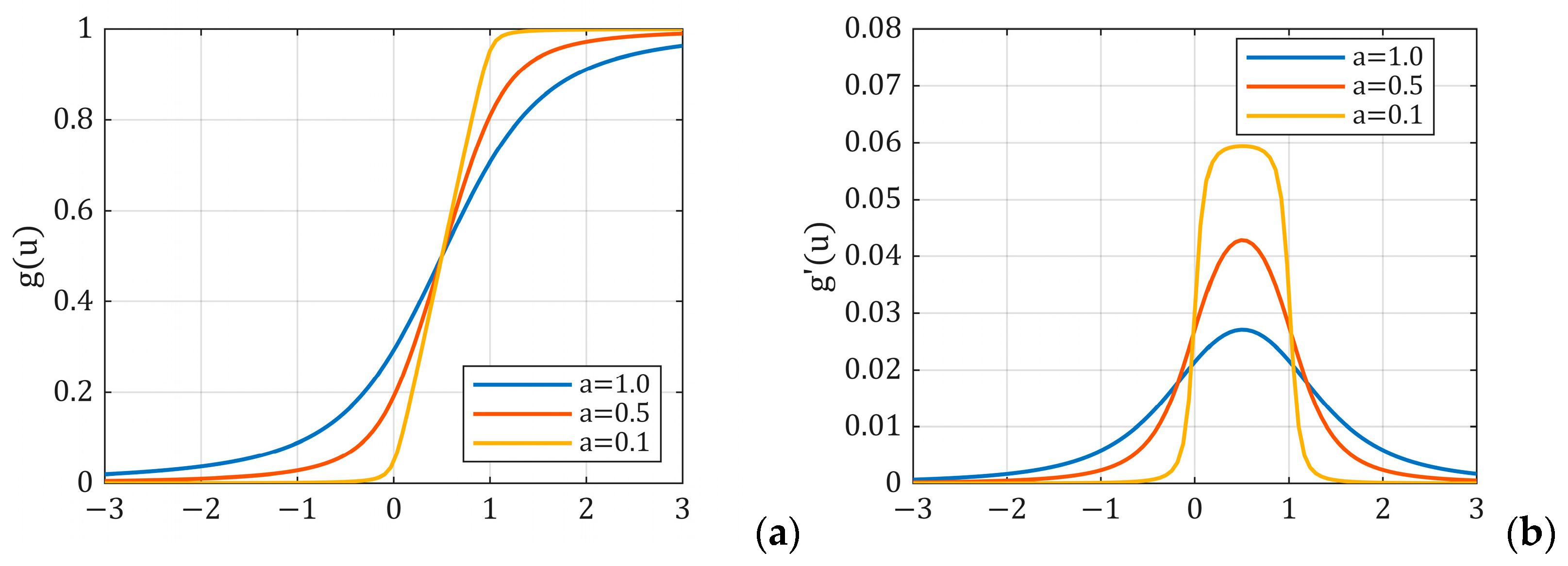
AP-DDP effectively tackles issues of premature convergence and low computational efficiency when control constraints are added to the existing DDP method. The main innovation of AP-DDP is the introduction of a relaxation coefficient that dynamically adjusts the smoothness of the projection function, enabling the optimization of control variable constraints. Figure 1 illustrates how different relaxation coefficients influence the projection function and the derivatives of the projection functions corresponding to different relaxation coefficients.

In the initial stage of the AP-DDP algorithm, a relatively large relaxation coefficient is assigned to the projection function. This makes the gradient not tend to zero when the control vector approaches the constraint boundary, and the algorithm will continue to update and reduce the risk of getting stuck in a local optimum. As the algorithm progresses, the relaxation coefficient gradually decreases, causing the boundary of the projection function to align with the constraints of the control variables, thus ensuring the accuracy of the results. Specifically, the projection function, including the relaxation coefficient, is as follows:

$$g(u)={\displaystyle \frac{1}{2}}(\underset{\_}{b}+\sqrt{{\lambda }^2+{\left(u-\underset{\_}{b}\right)}^2})+{\displaystyle \frac{1}{2}}(\overline{b}-\sqrt{{\lambda }^2+{\left(u-\overline{b}\right)}^2})$$

(10)

where $\lambda$ is the relaxation coefficient. To ensure that the relaxation coefficient gradually decreases during the iteration process, this paper uses a decay function with monotonic characteristics to establish the connection between the relaxation coefficient and the value function, achieving the adaptive iteration of the relaxation coefficient. The attenuation function is as follows:

$$\lambda =0.5\cdot {\displaystyle \frac{J_{current}}{J_0}}\cdot \exp (-{\displaystyle \frac{J_{current}}{J_0}})$$

(11)

where $J_0$ is the initial cost function and $J_{current}$ is the current cost function.

The decay function is composed of a linear term and a power term, and its derivative is as follows:

$${\lambda }^{\prime }=0.5\cdot \exp (-{\displaystyle \frac{J_{current}}{J_0}})\cdot (1-{\displaystyle \frac{J_{current}}{J_0}})$$

(12)

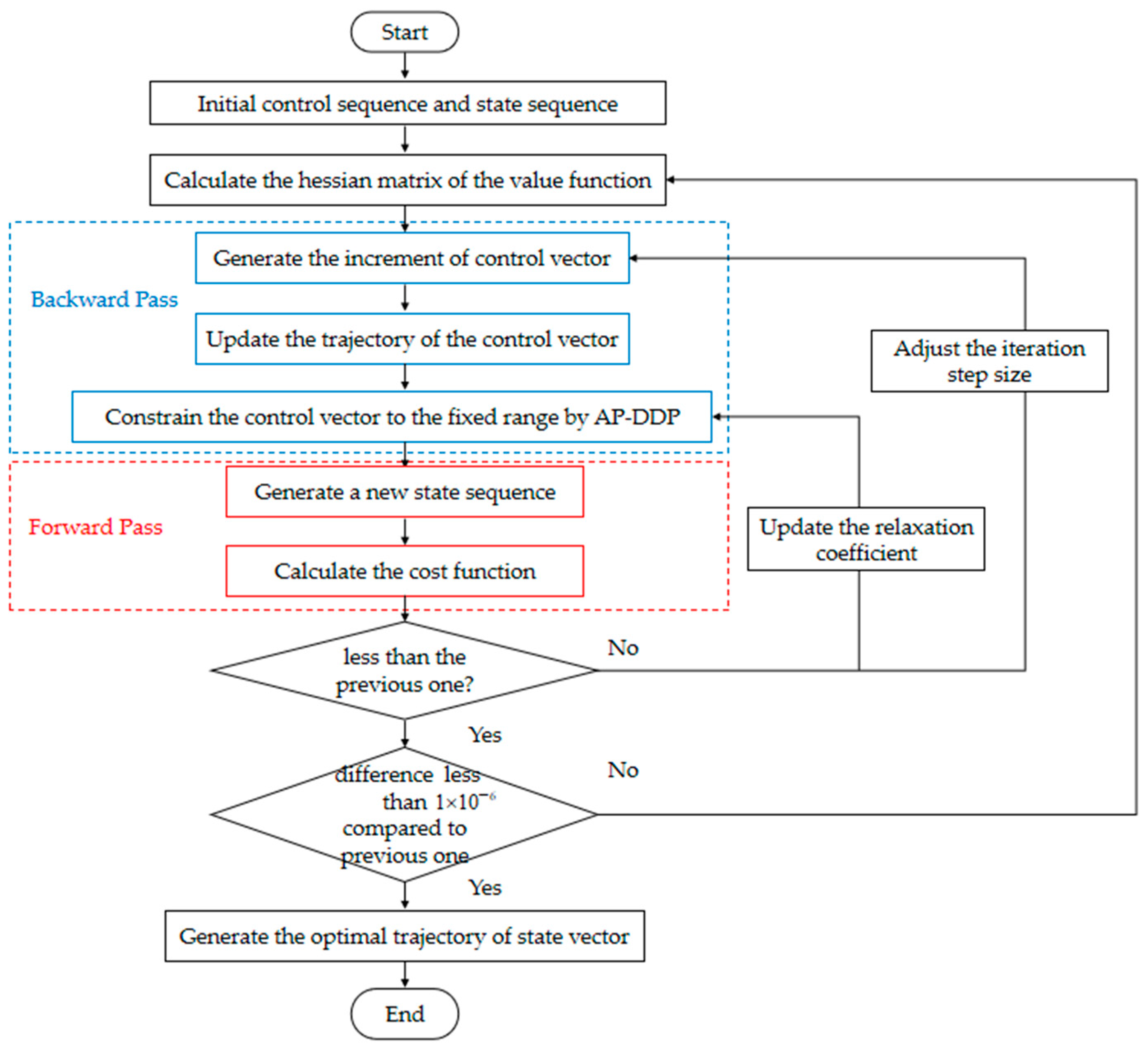
where $J_{current}$ is always smaller than $J_0$ during the iteration process; therefore, the derivative of the decay function is always positive, and the relaxation coefficient decreases as $J_{current}$ gradually decreases. As seen from Equation (11), the relaxation coefficient in this article gradually decreases from 0.5 to nearly 0. The framework of AP-DDP is shown in Figure 2.

Specifically, the iterative process of AP-DDP is divided into seven steps, as follows, and including two cycles.

Step 1: Initialize the state and control vectors each time, then generate the initial cost function.

Step 2: Compute the Hessian matrix of the value function at each time.

Step 3: Compute the control variable updates via backpropagation and produce the trajectory.

Step 4: Apply the AP-DDP method to restrict the control variable’s trajectory within a fixed interval.

Step 5: Generate the state variable trajectory by forward propagation using the constrained control variable trajectory, and then compute the new cost function.

Step 6: If the cost function is lower than the value calculated in the previous iteration, accept the current state variable trajectory; otherwise, use a linear search strategy to adjust the iteration step size, generate a new relaxation coefficient based on the decay function, and regenerate the control variable trajectory.

Step 7: Repeat steps 2 to 6 multiple times until the difference between the two iterations is less than $1\times {10}^{-6}$ (or another convergence criterion). Then, the optimal trajectory is considered to have been generated.

The advantage of the adaptive projection function is that it enhances its performance. Early in the iterations, a larger relaxation coefficient makes the projection function smoother, and the control increase is less likely to approach zero, allowing DDP to quickly reach the optimal solution and avoid getting stuck in local optima. As the iterations progress, the relaxation coefficient gradually decreases, enabling the control trajectory to reach the constraint boundary and improve the solution’s accuracy.

3.2. Linear Search Strategy

The AP-DDP method uses a line search strategy during the backward pass to ensure the algorithm converges to the optimal solution. The formula for the line search strategy is as follows:

$$\begin{array}{l}{u}_t^{new}=u_t-{\mathrm{Q}}_{uu}^{-1}{\mathrm{Q}}_{ux}\cdot (x_t^{new}-x_t)-\alpha \cdot {\mathrm{Q}}_{uu}^{-1}{\mathrm{Q}}_u\hfill \\ x_{t+1}^{new}=f(x_t^{new},u_t^{new})\hfill \end{array}$$

(13)

where $\alpha$ represents the line search step size; it is set to be within the range of 0 to 1 in this paper, and it is used to adjust the magnitude of the control strategy update during each iteration. Specifically, in each iteration, AP-DDP calculates the adjustment direction of the control strategy based on the local quadratic model. The step size is determined through a line search method (such as the Armijo criterion) to find an appropriate value that aligns the actual decrease in the loss function with the predicted reduction by the model. This mechanism can prevent divergence of the iteration or trajectory deviation caused by a huge step size and avoid slow convergence resulting from a tiny step size. Therefore, it balances the stability and efficiency of the algorithm.

4. Example Analysis

To evaluate the performance of the AP-DDP method, this section compares it with the truncated DDP, projected DDP, and Box-DDP methods using three examples. The first example solves for the optimal trajectory of a numerical equation, the second for a pendulum, and the third for a two-stage rocket. We determine the absolute error by comparing the terminal state of the trajectory generated by the AP-DDP method to the target state. The absolute error is described in Equation (14).

$$\epsilon ={\displaystyle \frac{1}{n}}{\displaystyle {\sum }_{i=1}^n\left|x_i-{\widehat{x}}_i\right|}$$

(14)

where $x_i$ represents the target state vector, ${\widehat{x}}_i$ represents the final state vector generated by the algorithm, and n is the dimension of the state variable. The experiment was conducted on a computing device with an i7-14650 processor which was designed and manufactured by Intel corporation of the United States, Windows 11 operating system, and 32 GB of RAM. We compared the differences among the various methods based on the absolute error and the computing time.

4.1. Example of Numerical Testing

The first example is to solve the optimal trajectory of a numerical equation. Its state equation involves three state vectors and one control vector, as shown in Equation (15).

$$\begin{array}{l}{x}^{\prime }=v\cdot \sin (u)\\ y^{\prime }=-v\cdot \cos (u)\\ v^{\prime }=g\cdot \cos (u)\end{array}$$

(15)

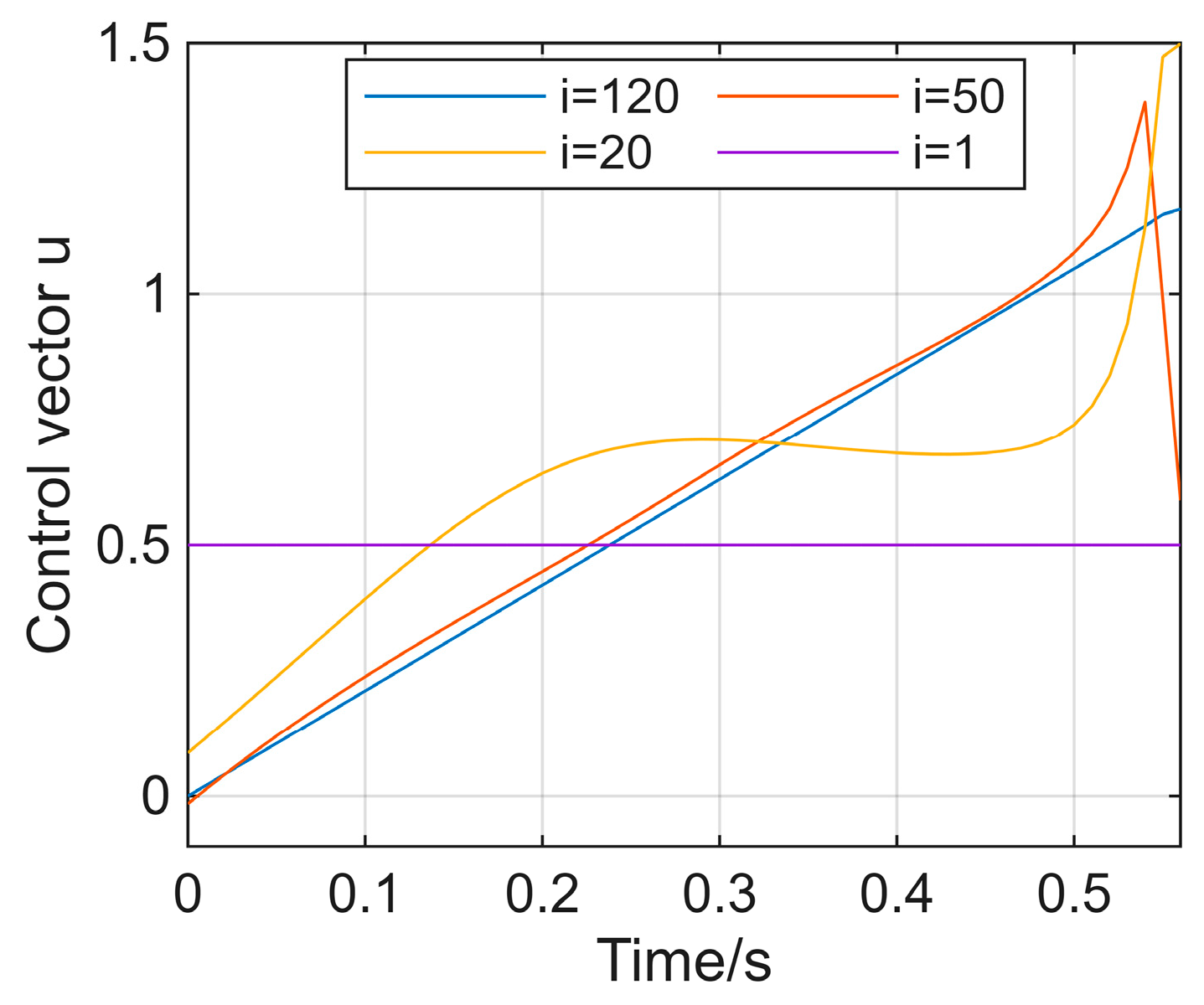
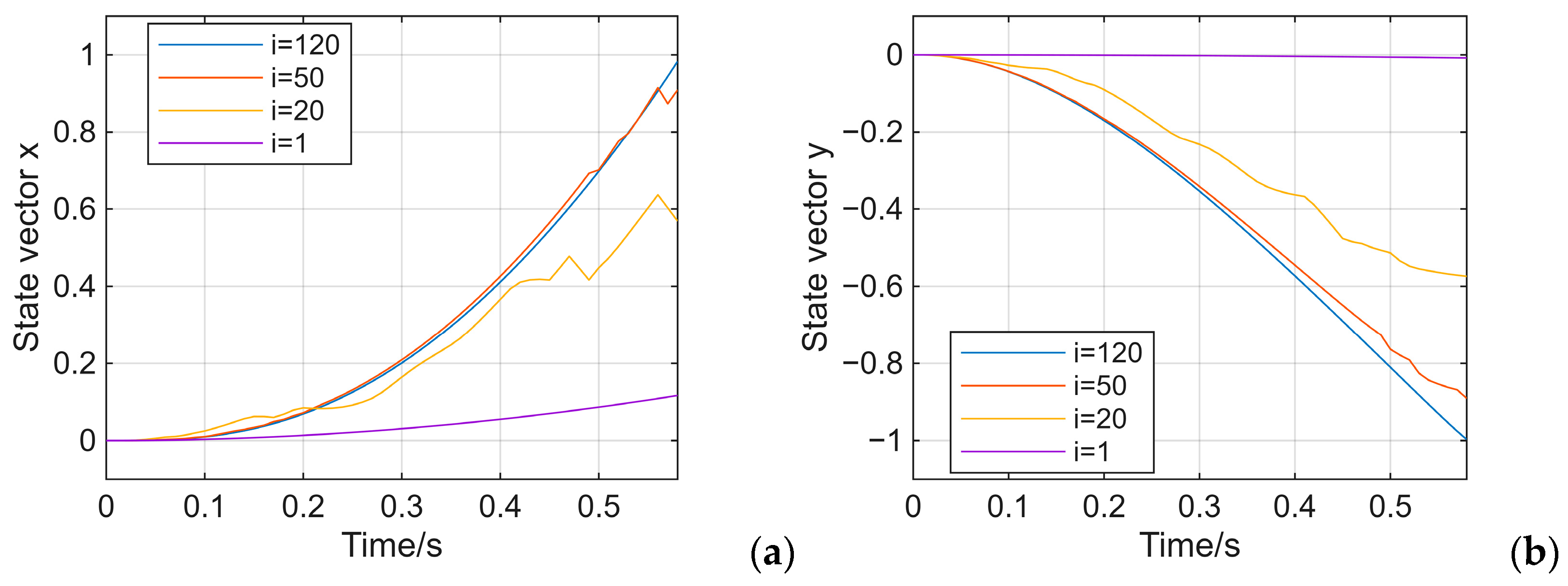
where $x$, $y$, and $v$ are three state vectors, u is the control vector, and its range is between −1.5 and 1.5. The initial state is [0, 0, 0], and the target state vectors are reached at [1, −1, Free] after 0.58 s; the first two state vectors must obtain the specified positions. We used the proposed AP-DDP method to constrain the control vector’s range and to generate the optimal trajectories for both the control and state vectors. The trajectory convergence of the control vector is shown in Figure 3, indicating that it remains within the constraints at all times. Figure 4 depicts the trajectory convergence of the state vectors, showing that, as the iterations progress, the final position of the state vector gradually approaches the target position. The final states produced by different trajectory optimization methods are listed in

Table 1. Comparison of the final state vectors and target state vectors of different trajectory optimization methods.

		Target	Truncated-DDP	Projection-DDP	Box-DDP	AP-DDP
State vectors	x	1.0	0.9806	0.9852	0.9827	0.9831
	y	−1.0	−1.0020	−0.9933	−0.9961	−0.9973
	v	Free	4.5171	4.4975	4.5039	4.5065

.

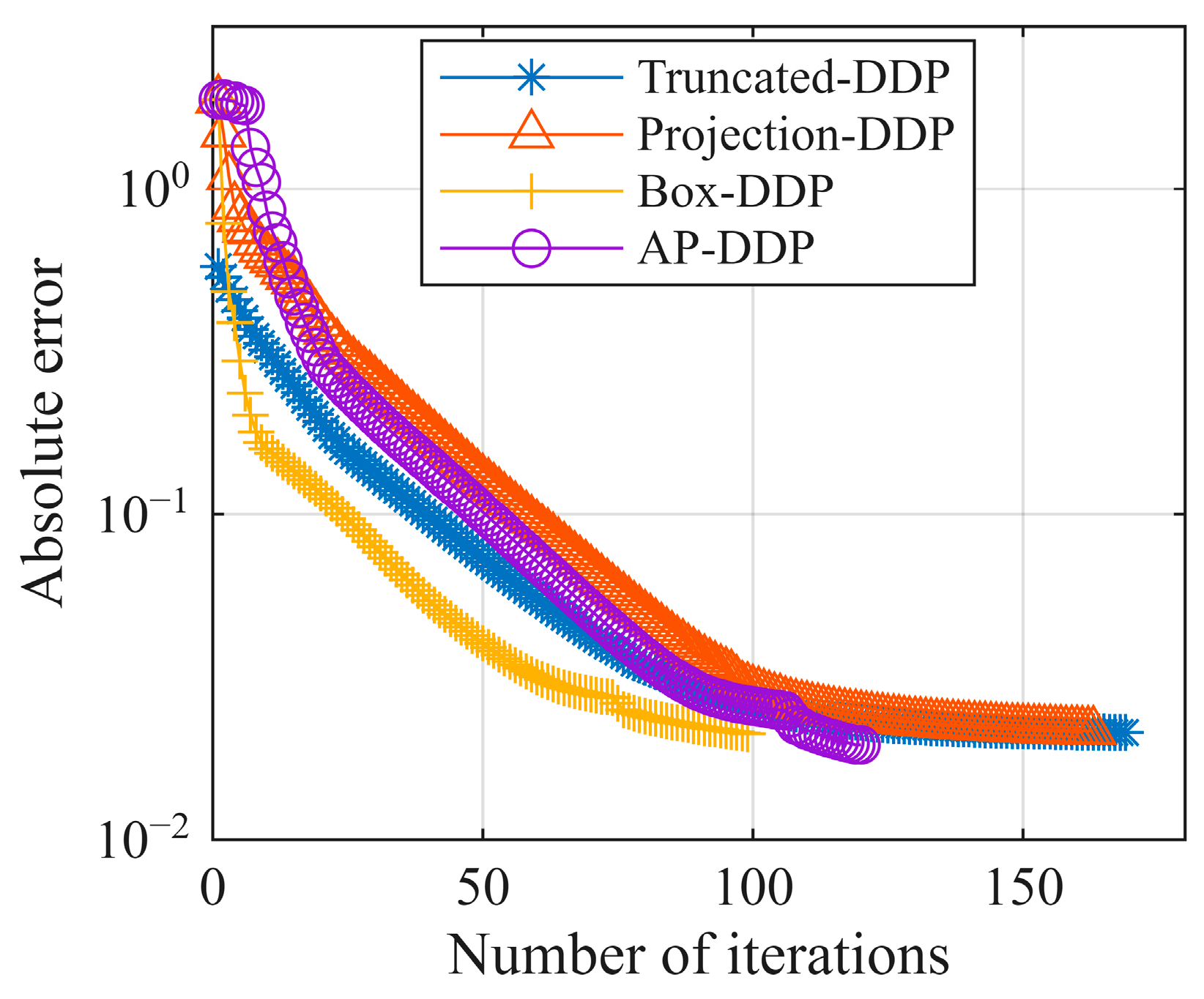
The absolute error and computational consumption are shown in

Table 2. Comparison of errors and computational consumption corresponding to different methods of the numerical example.

	Truncated-DDP	Projection-DDP	Box-DDP	AP-DDP
Absolute error	0.0214	0.0215	0.0212	0.0196
Variance	$3.804\times {10}^{-4}$	$2.639\times {10}^{-4}$	$3.145\times {10}^{-4}$	$2.929\times {10}^{-4}$
Standard deviation	0.0195	0.0162	0.0177	0.0171
Number of iterations	169	163	99	120
Time consumption(s)	4.21	3.93	21.99	2.64

and Figure 5. The results indicate that the absolute errors of all methods are around $1\times {10}^{-2}$. The final state vectors generated by the AP-DDP method are the closest to the target state vectors. Although the Box-DDP method has the least number of iterations, its computational process requires solving a quadratic programming sub-problem in each iteration, resulting in low computational efficiency and the highest computational consumption. Compared with the other three methods, the proposed AP-DDP method has the shortest computational time. It achieves higher computational efficiency while maintaining high computational accuracy.

4.2. Example of Pendulum

The second example is the pendulum, which consists of three state variables and one control variable. Its state equation is shown in Equation (16).

$$\begin{array}{l}\theta =\arctan (x/y)\\ {\theta }^{\prime }=v\\ v^{\prime }=-3\cdot 9.8*\sin (\theta )/2+3\cdot u/2\\ x=\sin (\theta )\\ y=\cos (\theta )\end{array}$$

(16)

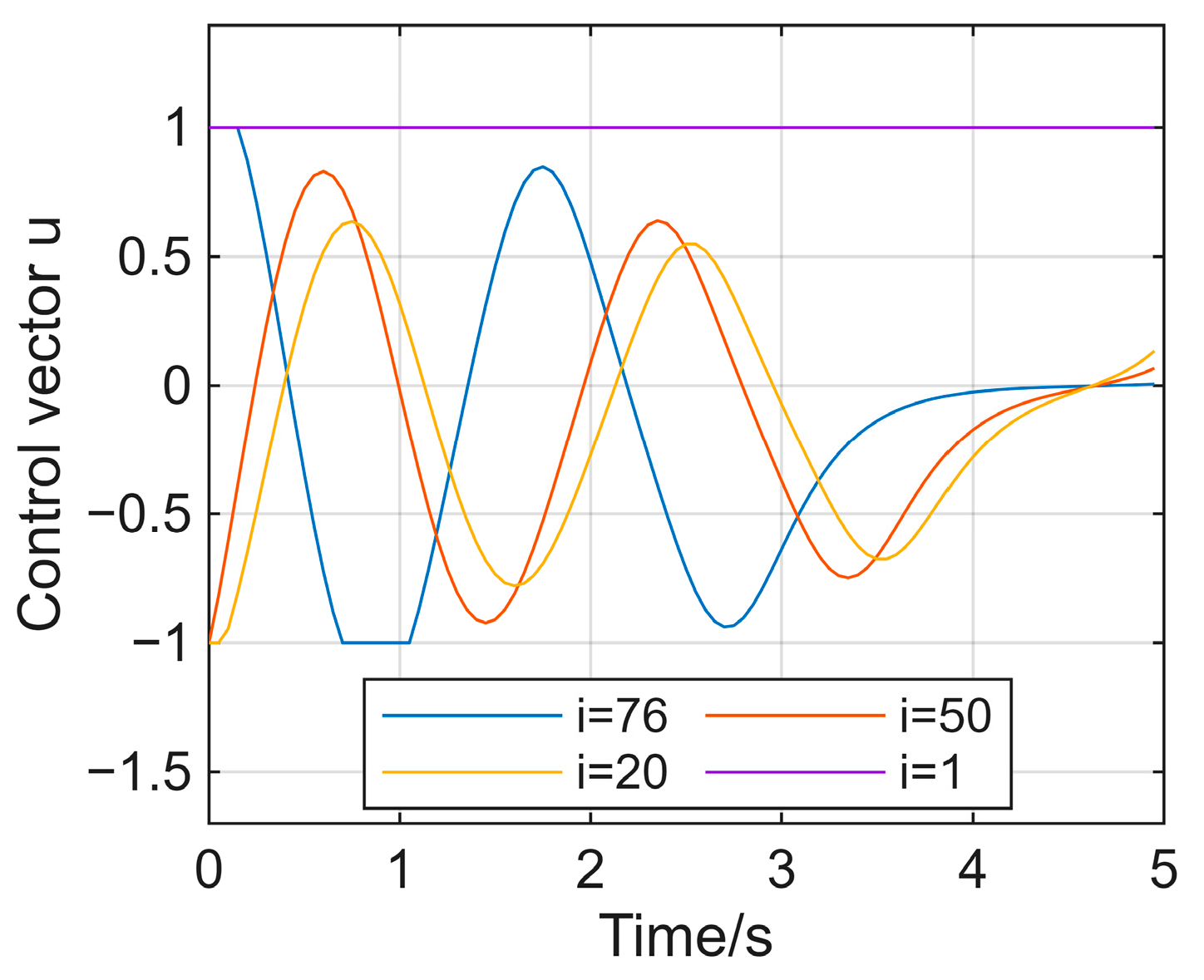
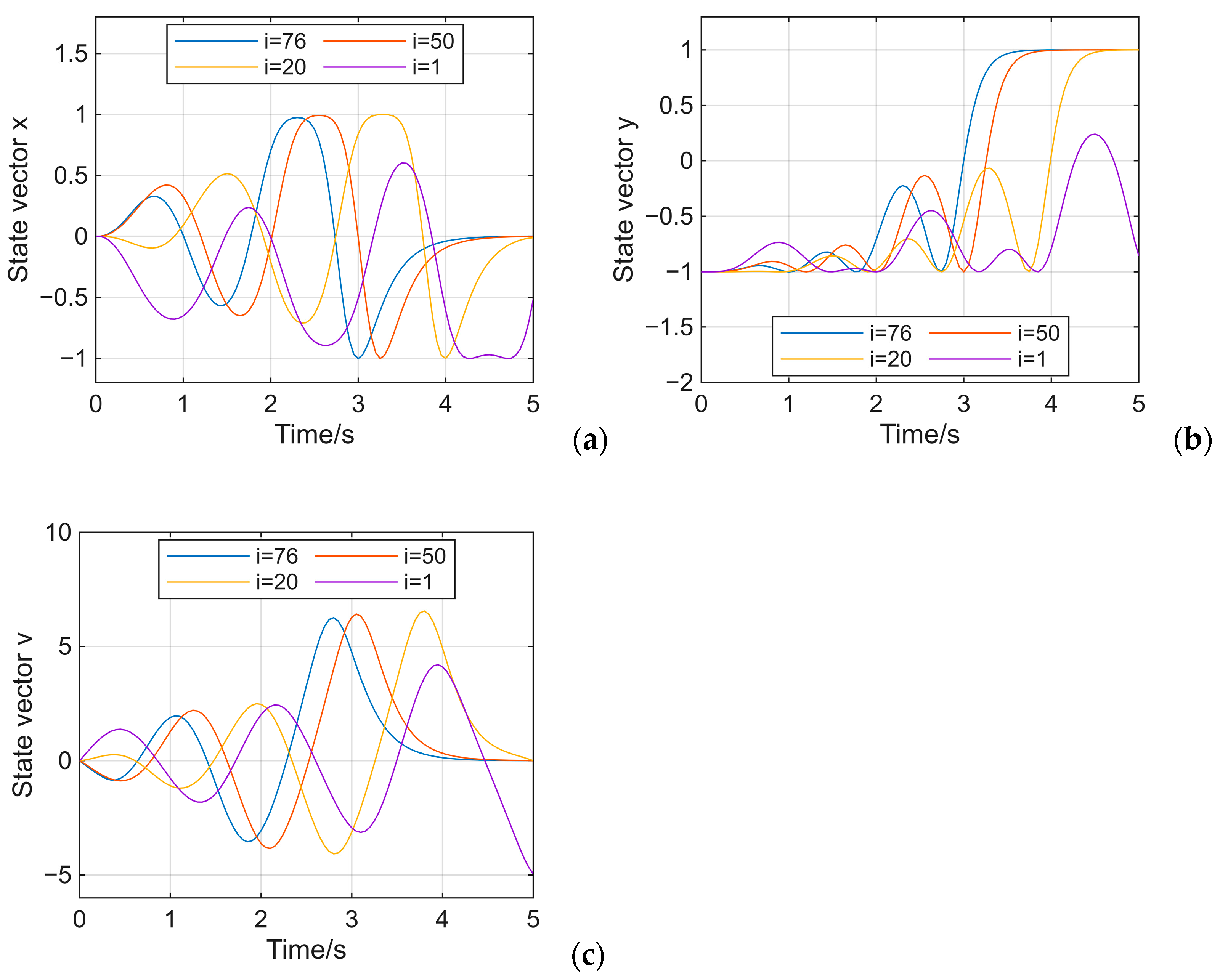
where $x$, $y$, and $v$ are three state vectors, u is the control vector, and $\theta$ represents the angle used as an intermediate vector to solve the state vectors x and y. The range of the control vector is between −1.0 and 1.0. The initial state is [0, −1, 0], and the objective state vectors reached [0, 1, 0] after 5 s. We employed the proposed AP-DDP method to limit the range of the control vector and to generate the optimal trajectories of the control vector and state vectors. The trajectory convergence process of the control vector is shown in Figure 6. It can be seen that the control vector is always within the constraints. Figure 7 illustrates the trajectory convergence process of the state vectors. It can be seen that, as the iterations proceed, the final position of the state vector gradually approaches the target position. The final states generated by different trajectory optimization methods are shown in

Table 3. Comparison of the final state vectors and the target state vectors of different trajectory optimization methods.

		Target	Truncated-DDP	Projection-DDP	Box-DDP	AP-DDP
State vectors	x	1.0	$-5.28\times {10}^{-4}$	$-3.8\times {10}^{-3}$	$-7.06\times {10}^{-4}$	$-4.19\times {10}^{-4}$
	y	−1.0	1.0	1.0	1.0	1.0
	v	0	$1.09\times {10}^{-4}$	0.0012	$1.47\times {10}^{-4}$	$8.30\times {10}^{-5}$

.

Table 4. Comparison of errors and computational consumption corresponding to different methods of the pendulum.

	Truncated-DDP	Projection-DDP	Box-DDP	AP-DDP
Absolute error	$6.37\times {10}^{-4}$	$5.0\times {10}^{-3}$	$8.53\times {10}^{-4}$	$5.02\times {10}^{-4}$
Variance	$2.901\times {10}^{-7}$	$1.588\times {10}^{-5}$	$5.20\times {10}^{-7}$	$1.824\times {10}^{-7}$
Standard deviation	$5.39\times {10}^{-4}$	$3.98\times {10}^{-3}$	$7.21\times {10}^{-4}$	$4.27\times {10}^{-4}$
Number of iterations	91	103	95	76
Time consumption(s)	1.13	1.24	3.96	0.98

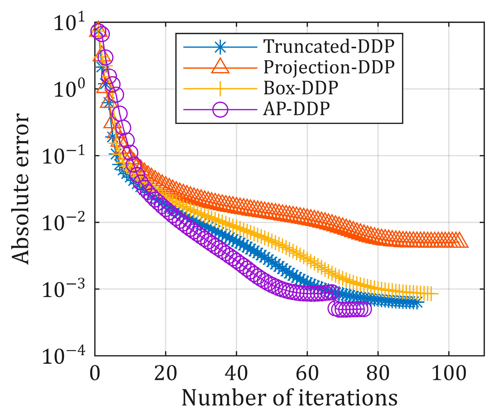
and Figure 8 show the absolute errors and computational costs, respectively. The results indicate that the absolute errors of all methods are around $1\times {10}^{-3}$. Table 4 and Figure 7 show the specific number of iterations, Figure 7 and Table 4 show that the AP-DDP method achieves the smallest absolute error, and its number of iterations and computing time are also the least.

4.3. Example of Trajectory Optimization for a Two-Stage Rocket

The third example is the trajectory optimization of a two-stage rocket. During the flight, the missile’s first stage sends the rocket to a certain altitude, separating it from the second stage. The rocket’s second stage continues to fly, sending the satellite to the predetermined orbit. The state equation of the two-stage rocket is expressed as Equation (17) in the geocentric rectangular inertial coordinate system.

$$\begin{array}{l}{r}^{\prime }=v\\ v^{\prime }=-{\displaystyle \frac{\mu }{{‖r‖}^3}}\cdot r+{\displaystyle \frac{T}{m}}\cdot u+{\displaystyle \frac{D}{m}}\\ m^{\prime }=-{\displaystyle \frac{T}{g_0{I}_{sp}}}\end{array}$$

(17)

where $r$ represents the three-dimensional coordinates of the rocket’s position, $v$ represents the three-dimensional velocity of the rocket, $\mu$ is the gravitational parameter, $T$ is the rocket’s thrust, where the first-stage rocket is equipped with nine engines and the second-stage rocket is equipped with one engine, $D$ represents the air resistance in three directions of the rocket, $m$ is the rocket’s mass (gradually decreasing as fuel is consumed), $g_0$ is the gravitational acceleration corresponding to the initial position, and $I_{sp}$ is the specific impulse of the engine. When the separation occurs, the first-stage rocket detaches from the entire rocket. Subsequently, the rocket’s mass will suddenly change, and the initial mass after the separation is the mass of the second-stage rocket. The calculation for air resistance is shown in Equation (18).

$$\begin{array}{l}D=-{\displaystyle \frac{1}{2}}\cdot \rho \cdot S\cdot C_D\cdot v^2\\ \rho ={\rho }_0\cdot \exp (-h/H)\\ h=‖r‖-R_e\end{array}$$

(18)

where $\rho$ represents the air density which varying with altitude, $S$ represents the contact area, $C_D$ represents the drag coefficient, ${\rho }_0$ represents the initial air density, $h$ represents the altitude, $H$ represents the standard density altitude, and $R_e$ represents the radius of the Earth. As the rocket’s altitude decreases, the air density decreases, and the corresponding air resistance decreases. Additionally, the control vectors’ limits, the components of the rocket’s thrust in three directions, must be considered. To maintain control stability, it is assumed that the missile always operates at maximum power, meaning the sum of the squares of the thrust components equals 1, as shown in Equation (19):

$${‖u‖}^2=u_x^2+u_y^2+u_z^2=1$$

(19)

where $u_x,u_y,u_z$ represent the components of the thrust in the three directions. Two of them are selected as control vectors, and their value ranges are between 0 and 1. The objective function is to minimize the distance between the final state vectors and the target state vectors. Six parameters of the orbit determine the target state vectors, and the operating time of the first-stage rocket is 130 s, while that of the second-stage rocket is 350 s. The specific parameters for optimizing the rocket’s orbit are shown in

Table 5. Parameters required for the rocket trajectory optimization.

Parameter	Value	Parameter	Value
The mass of the first-stage rocket (kg)	431,600	Semi-major axis (km)	7083.6
The mass of the second-stage rocket (kg)	107,500	Eccentricity	0.1670
Initial position	(6023.4, 0, 2097.6)	Inclination (rad)	0.4279
Gravitational acceleration (m·s−2)	9.807	Right ascension (rad)	5.6998
Maximum stress coefficient (kpa)	80	Argument of periapsis (rad)	5.8564
Maximum acceleration (m/s2)	100	True anomaly (rad)	1.2667
Gravity parameter	$3.986\times {10}^{14}$	Resistance coefficient	0.5
The radius of the Earth (km)	6378.1	Density standard height (m)	7200
Thrust specific impulse of the engine	340	Engine thrust (N)	934,000

.

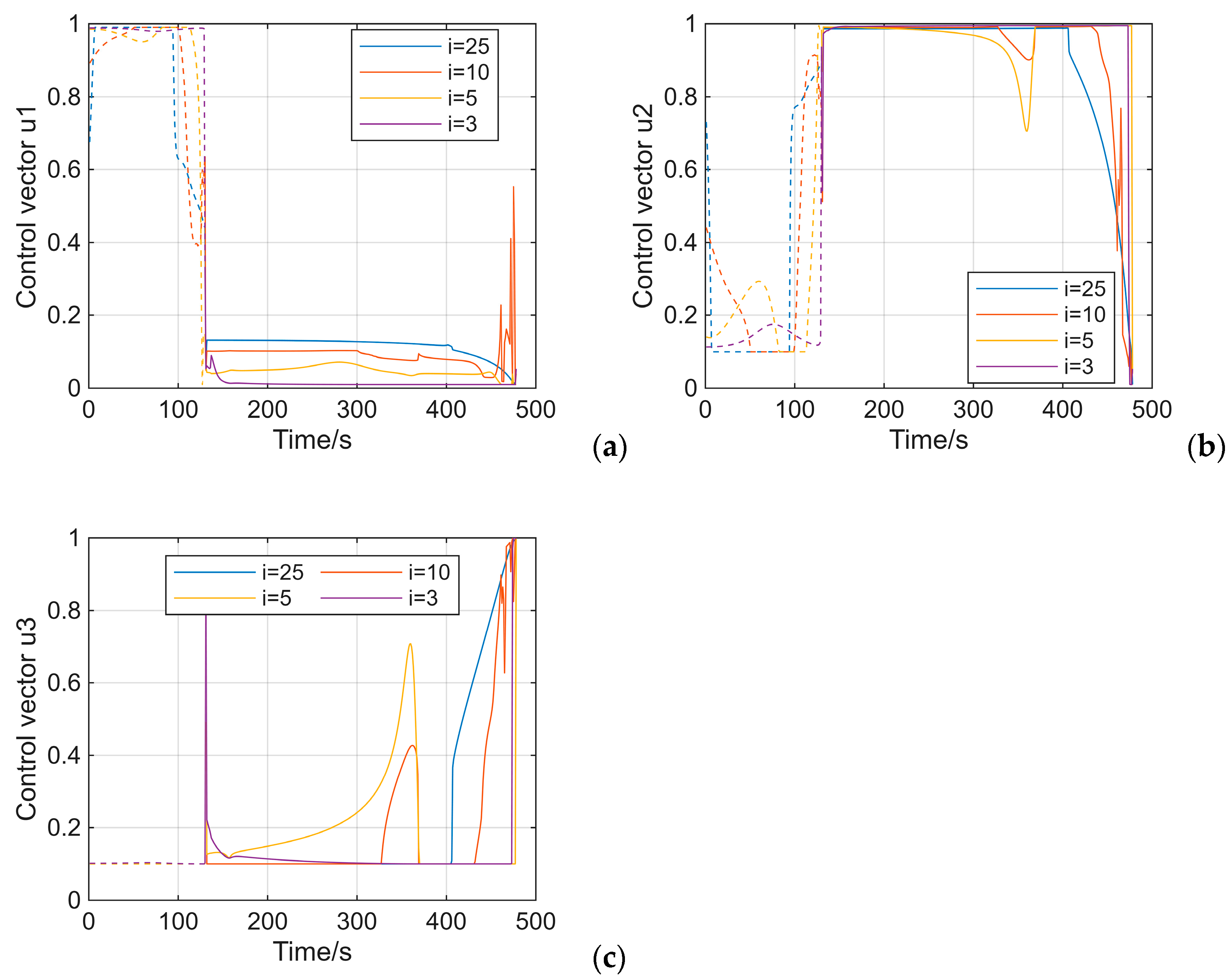
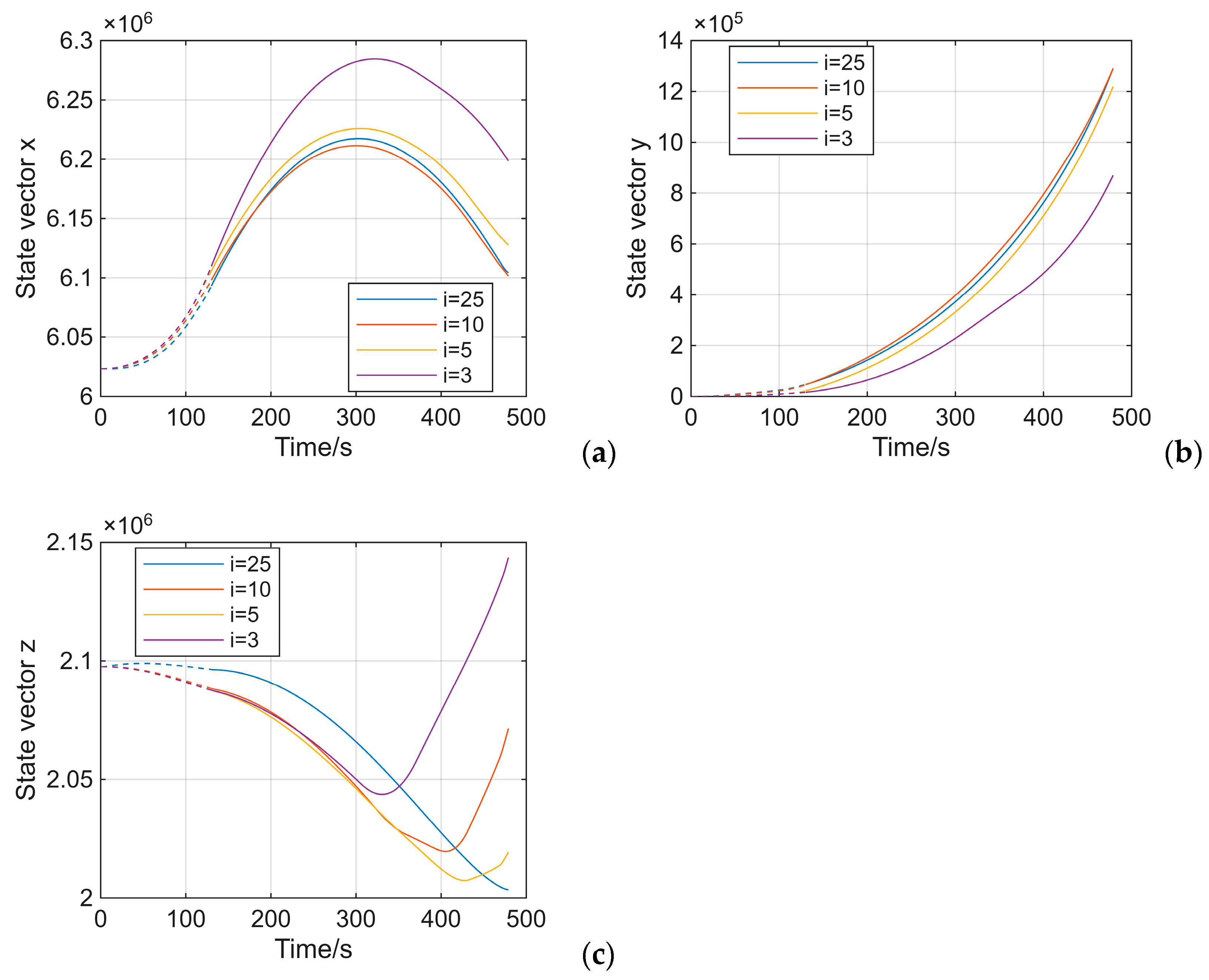
We used the proposed AP-DDP method to restrict the control vector’s range and to generate the optimal control and state trajectories. Figure 9 shows the control vector’s trajectory convergence process, demonstrating that it always remains within the constraints. Figure 10 illustrates the trajectory convergence process of the state vectors, showing that, as the iterations progress, the final position of the state vector gradually approaches the target position. The final states produced by different trajectory optimization methods are listed in

Table 6. Comparison of the final state vectors and target state vectors corresponding to different methods of the rocket.

		Target	Truncated-DDP	Projection-DDP	Box-DDP	AP-DDP
State vectors	x	6,100,869.48	6,100,870.14	6,128,518.29	6,100,870.09	6,100,869.66
	y	1,296,779.84	1,296,779.84	1,233,028.36	1,296,779.84	1,296,779.82
	z	2,026,578.26	2,026,578.25	2,119,693.18	2,026,578.22	2,026,578.13

.

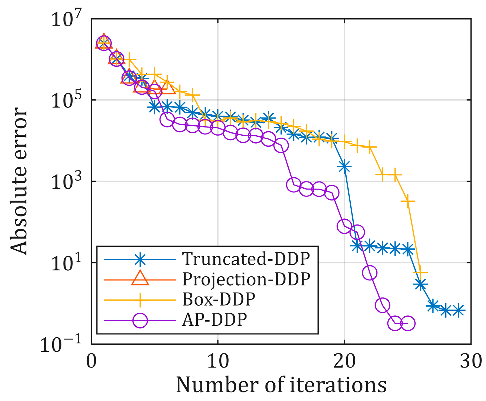
The absolute error and computational cost are shown in

Table 7. Comparison of errors and computational consumption corresponding to different methods of the rocket.

	Truncated-DDP	Projection-DDP	Box-DDP	AP-DDP
Absolute error	0.676	$1.85\times {10}^5$	0.650	0.3226
Variance	0.4357	$1.35\times {10}^{10}$	0.3737	0.0497
Standard deviation	0.660	$1.162\times {10}^5$	0.6113	0.2229
Number of iterations	29	-	26	25
Time consumption(s)	6.94	-	20.88	5.64

and Figure 11, respectively. The results indicate that the projection-DDP method has a significant mistake and has fallen into a local optimum. The other three methods have minor errors, while the AP-DDP method proposed in this paper has the fewest errors. The truncated DDP, Box-DDP, and AP-DDP methods converged to the global optimum after 29, 26, and 25 cycles, respectively. The AP-DDP method had the fewest iterations and the shortest computational time. This demonstrates that the AP-DDP algorithm has higher computational efficiency while maintaining high accuracy.

5. Conclusions

This paper proposes the AP-DDP method to address the issue of missing control variable constraints in the trajectory optimization problems solved by the traditional DDP method. The AP-DDP method prevents the issue of gradient disappearance near constraint boundaries in control variables, which can cause the algorithm to get stuck in local optima, thereby improving stability. Additionally, using larger relaxation coefficients during the initial optimization stage accelerates exploring feasible solutions and boosts the algorithm’s efficiency. We compared the AP-DDP method with similar methods across three test cases. The results show that the final state vectors obtained by the AP-DDP method are the closest to the target state vectors, requiring less computational effort. While ensuring the iterative process reaches the global optimum, the computing time of the AP-DDP method was reduced by 32.8%, 13.3%, and 18.5%, respectively, in the three examples. This confirms the efficiency of this method in solving constrained optimal control problems. Subsequent research will explore the combination of the AP-DDP method with reliability and robustness approaches, ultimately achieving the reliable control of aircraft and robots in the presence of external environmental disturbances.

References

1. Song, Z.Y.; Liu, L.D.; Chen, X.F.; Xu, S.; Wu, Y. Development and key technologies of the new generation medium launch vehicle Long March 8. J. Astronaut. 2023, 44, 476–485. [Google Scholar]
2. Nyborg, K.; Anderson, M.C.; Gee, K.L. Turbulence-induced variability of a far-field Falcon-9 sonic boom measurement. J. Acoust. Soc. Am. 2024, 155, A256–A257. [Google Scholar] [CrossRef]
3. Rao, A.V. A Survey of Numerical Methods for Optimal Control. Adv. Astronaut. Sci. 2010, 135, 497–528. [Google Scholar]
4. Gidas, B.; Ni, W.M.; Nirenberg, L. Symmetry and related properties via the maximum principle. Commun. Math. Phys. 1979, 68, 209–243. [Google Scholar] [CrossRef]
5. Liu, T.; Zhang, Y.; Yin, X.; He, W. Aviation Fuel Pump Fault Diagnosis Based on Conditional Variational Self-Encoder Adaptive Synthetic Less Data Enhancement. Mathematics 2025, 13, 2218. [Google Scholar] [CrossRef]
6. He, B. Rocket Flight Parameter Optimization Design Based on Improved Genetic Algorithm. Ph.D. Thesis, Nanjing University of Science and Technology, Nanjing, China, 2020. [Google Scholar]
7. Cui, N.G.; Guo, D.Z.; Li, K.Y.; Wei, C. Survey of numerical methods for spacecraft trajectory optimization. Tactical Missile Technol. 2020, 05, 38–75. [Google Scholar] [CrossRef]
8. Liu, Z.; Lu, H.R.; Zheng, W.; Wen, G.; Wang, Y.; Zhou, X. Fast time-cooperative trajectory planning for multiple gliding vehicles. Acta Aeronaut. Astronaut. Sin. 2021, 42, 524497. [Google Scholar]
9. Tian, B.L.; Li, Z.Y.; Wu, S.Y.; Zong, Q. Review of reentry trajectory and guidance and control methods for reusable launch vehicles. Acta Aeronaut. Astronaut. Sin. 2020, 41, 624072. [Google Scholar]
10. Rao, A.V.; Benson, D.A.; Darby, C.; Patterson, M.A.; Francolin, C.; Sanders, I.; Huntington, G.T. Algorithm 902: GPOPS, A MATLAB software for solving multiple-phase optimal control problems using the gauss pseudospectral method. ACM Trans. Math. Softw. 2010, 37, 1–39. [Google Scholar] [CrossRef]
11. Jiang, R.Y.; Chao, T.; Wang, S.Y.; Yang, M. Pseudospectral method solving low-thrust orbit for deep space exploration. J. Syst. Simul. 2017, 29, 2043–2053. [Google Scholar]
12. Zhang, Z.G.; Yu, M.L.; Geng, G.Y.; Song, Q. Research on online guidance method for launch vehicle using pseudospectral method. J. Astronaut. 2017, 38, 262–269. [Google Scholar]
13. Ma, L.; Wang, K.; Shao, Z.; Song, Z.; Biegler, L.T. Direct trajectory optimization framework for vertical takeoff and vertical landing reusable rockets: Case study of two-stage rockets. Eng. Optim. 2018, 51, 627–645. [Google Scholar] [CrossRef]
14. Bertsekas, D.P. Reinforcement Learning and Optimal Control; Li, Y.C., Translator; Tsinghua University Press: Beijing, China, 2020. [Google Scholar]
15. Wang, Q.M.; Jiang, J.Y.; Lyu, Z.C.; Zhang, H.Z. Research on cooperative adaptive cruise control strategy based on improved MPC. J. Syst. Simul. 2022, 34, 2087–2097. [Google Scholar]
16. Li, J.Q. Research on Trajectory Optimization and Guidance for Vertical Recovery of Reusable Rocket Boosters. Ph.D. Thesis, Huazhong University of Science and Technology, Wuhan, China, 2023. [Google Scholar]
17. Mastalli, C.; Budhiraja, R.; Merkt, W.; Saurel, G.; Hammoud, B.; Naveau, M.; Carpentier, J.; Righetti, L.; Vijayakumar, S.; Mansard, N. Crocoddyl: An Efficient and Versatile Framework for Multi-Contact Optimal Control. In Proceedings of the 2020 IEEE International Conference on Robotics and Automation, Paris, France, 31 May–31 August 2020. [Google Scholar]
18. Cao, K.; Cao, M.; Yuan, S.; Xie, L. DIRECT: A Differential Dynamic Programming Based Framework for Trajectory Generation. IEEE Robot. Autom. Lett. 2022, 7, 2439–2446. [Google Scholar] [CrossRef]
19. Xie, Z.; Liu, C.K.; Hauser, K. Differential dynamic programming with nonlinear constraints. In Proceedings of the 2017 IEEE International Conference on Robotics and Automation, Singapore, 29 May–3 June 2017. [Google Scholar]
20. Sleiman, J.P.; Farshidian, F.; Hutter, M. Constraint Handling in Continuous-Time DDP-Based Model Predictive Control. In Proceedings of the 2021 IEEE International Conference on Robotics and Automation, Xi’an, China, 30 May–5 June 2021. [Google Scholar]
21. Howell, T.A.; Jackson, B.E.; Manchester, Z. ALTRO: A Fast Solver for Constrained Trajectory Optimization. In Proceedings of the 2019 IEEE/RSJ International Conference on Intelligent Robots and Systems, Macau, China, 3–8 November 2019. [Google Scholar]
22. Mastalli, C.; Merkt, W.; Marti-Saumell, J.; Ferrolho, H.; Solà, J.; Mansard, N.; Vijayakumar, S. A feasibility-driven approach to control-limited DDP. Auton. Robot. 2022, 46, 985–1005. [Google Scholar] [CrossRef]
23. Marti-Saumell, J.; Solà, J.; Mastalli, C.; Santamaria-Navarro, A. Squash-Box Feasibility Driven Differential Dynamic Programming. In Proceedings of the 2020 IEEE/RSJ International Conference on Intelligent Robots and Systems, Las Vegas, NV, USA, 24 October–24 January 2021. [Google Scholar]
24. Aoyama, Y.; Boutselis, G.; Patel, A.; Theodorou, E.A. Constrained Differential Dynamic Programming Revisited. In Proceedings of the 2021 International Conference on Robotics and Automation, Yokohama, Japan, 30 May–5 June 2021. [Google Scholar]
Figure 1. The influence of different relaxation coefficients on the projection function. (a) The influence of different relaxation coefficients on the projection function. (b) The influence of different relaxation coefficients on the derivative of the projection function.
Mathematics 13 02637 g001
Figure 2. The framework of the AP-DDP method.
Mathematics 13 02637 g002
Figure 3. The trajectory update process of the control vector for the numerical example.
Mathematics 13 02637 g003
Figure 4. The trajectory update process of the state vectors for the numerical example. (a) The trajectory update process of the state vectors x for the numerical example. (b) The trajectory update process of the state vectors y for the numerical example.
Mathematics 13 02637 g004
Figure 5. The iterative processes corresponding to different methods of the numerical example.
Mathematics 13 02637 g005
Figure 6. The trajectory update process of the control vector for the pendulum.
Mathematics 13 02637 g006
Figure 7. The trajectory update process of the state vectors for the pendulum. (a) The trajectory update process of the state vectors x for the pendulum. (b) The trajectory update process of the state vectors y for the pendulum. (c) The trajectory update process of the state vectors v for the pendulum.
Mathematics 13 02637 g007
Figure 8. The iterative processes corresponding to different methods of the pendulum.
Mathematics 13 02637 g008
Figure 9. The trajectory update process of the control vectors for the rocket. (a) The trajectory update process of the control vectors u1 for the rocket. (b) The trajectory update process of the control vectors u2 for the rocket. (c) The trajectory update process of the control vectors u3 for the rocket.
Mathematics 13 02637 g009
Figure 10. The trajectory update process of the state vectors for the rocket. (a) The trajectory update process of the state vectors x for the rocket. (b) The trajectory update process of the state vectors y for the rocket. (c) The trajectory update process of the state vectors z for the rocket.
Mathematics 13 02637 g010
Figure 11. The iterative processes corresponding to different methods of the rocket.
Mathematics 13 02637 g011