Abstract
The voltage source converters convert the DC to AC in order to interface distributed generation units with the utility grid, typically using an LCL filter to smooth the modulated wave. However, the LCL filter can introduce resonance, potentially cause instability, and necessitate the use of damping techniques, such as active damping, which utilizes feedback from the current control loop to suppress resonance. This paper presents a comprehensive performance assessment of four current-feedback-based active damping (AD) techniques—converter current feedback (CCF), CCF with capacitor current feedback (CCFAD), grid current feedback (GCF), and GCF with capacitor current feedback (GCFAD)—under a broad range of realistic grid disturbances and low switching frequency conditions. Unlike prior works that often analyze individual feedback strategies in isolation, this study highlights and compares their dynamic behavior, robustness, and total harmonic distortion (THD) in eight operational scenarios. The results reveal the severe instability of GCF in the absence of damping and the superior inherent damping property of CCF while demonstrating the comparable effectiveness of GCFAD. Moreover, a simplified yet robust design methodology for the LCL filter is proposed, enabling the filter to maintain stability and performance even under significant variations in grid impedance. Additionally, a sensitivity analysis of switching frequency variation is included. The findings offer valuable insights into selecting and implementing robust active damping methods for grid-connected converters operating at constrained switching frequencies. The effectiveness of the proposed methods has been validated through both MATLAB/Simulink simulations and hardware-in-the-loop (HIL) testing.
MSC:
93C10
1. Introduction
Due to its environmentally beneficial and sustainable properties, the distributed generation based on renewable energy has garnered much interest, offering a practical solution to future energy shortages and environmental degradation [1]. Grid-connected VSCs are essential in ensuring the safe, reliable, and high-quality operation of distributed generation units, since they serve as the mediator for energy conversion in the middle of distributed generation units and the utility grid [1,2]. To attenuate harmonics induced via the switching behavior of the VSC, a filtering stage is required [3]. VSCs rely on passive filters to provide this coupling and mitigate the switching frequencies, as they have low sensitivity to the system component values compared to active filters [4]. Typically, there are two options: LCL and L filter. A capacitor and two inductors make up the LCL filter, whereas a single inductor constitutes the L filter.
The L-filter is a first-order filter that provides an attenuation rate of 20 dB per decade throughout the frequency spectrum, so it is used with VSCs that have high switching frequencies; however, its inductance significantly reduces the overall system dynamics [5]. The L filters have a straightforward construction and require only minimal control methods. By utilizing more complex control schemes like proportional–repetitive and proportional–resonant, it is also possible to achieve greater closed-loop effectiveness [4]. Due to the large size required for L filters to meet standards, like IEEE 519 [6] and IEEE 1547 [7], and their limited suitability for high-power applications, LCL filters have gained focus as a solution, offering advantages such as lightweight, low cost, excellent high-frequency harmonic attenuation, superior filter and grid impedance decoupling, and operation at a lower switching frequency [5,8,9]. LCL filters exhibit resonance frequencies that require damping methods to prevent system instability, as improper damping of the resonant frequencies may result in grid current oscillations [10].
The researchers in [4] conducted a comparative evaluation of L and LCL filters in single-phase grid-tied power converters for active power injection, focusing on their ability to mitigate high-frequency harmonics. The study presents the state-space modeling and transfer functions of both filters, incorporating parasitic resistance effects, and utilizes a single-phase H-bridge inverter with unipolar PWM for numerical simulations. The findings indicate that, while L filters offer simplicity in implementation and control, they require large inductance values or higher switching frequencies to achieve acceptable current ripple, leading to increased power losses and reduced efficiency. In contrast, LCL filters provide superior attenuation of switching harmonics with smaller passive component values, reducing power losses and system size. However, LCL filters introduce stability challenges that necessitate damping mechanisms—either passive, which increases power losses, or active, which complicates control. The study concludes that the choice between L and LCL filters depends on the specific application, trade-offs between simplicity, efficiency, and harmonic performance. In the study of [8], the authors evaluate and compare L, LC, and LCL filters used in grid-connected VSCs, focusing on their ability to mitigate harmonics generated by semiconductor switching. The study highlights the increasing penetration of distributed generation (DG) and the necessity of high-quality power injection into the grid. While L and LC filters have been traditionally used, their required inductance values become impractical and costly at lower switching frequencies. The research finds that LCL filters provide a more efficient alternative, offering superior harmonic attenuation with lower component values, making them more economical. However, the study also emphasizes that LCL filters introduce resonance issues due to the presence of two inductors, requiring effective damping strategies to maintain stability.
Resonance issues are typically addressed using either passive damping (PD) or active damping (AD) techniques [11,12,13,14]. The PD approach with resistors is straightforward and cost-effective, but it reduces the ability to filter high-frequency harmonics and causes power losses [15], while the AD increases control complexity as it requires additional sensors, which may introduce noise problems because the differentiator amplifies high-frequency signals [5,16]. There are different types of AD techniques [17], such as filter-based, involving placing a digital filter alongside the current controller [18]; weighted average, utilizing the weighted average of the converter side and the grid side currents to prevent resonance [19]; and feedback-based, where the feedback states can be the capacitor current [11,20,21,22,23], the converter current (CCF) [12,13], the grid current (GCF) [14,24,25], or a combination of several different states [26,27,28].
Feedback-based AD techniques are straightforward, adaptable, and efficient; however, they necessitate high-accuracy sensors [2,14]. To address this, non-sensor-based estimation techniques have been suggested to acquire the required information [12,14]. The proportional capacitor current feedback and derivative capacitor voltage feedback are evaluated in the study of [20], concluding that only capacitor current feedback maintains system stability at high resonance frequencies, whereas both types of feedback are effective at midrange resonance frequencies. The capacitor current feedback is simple to implement, functioning as a virtual resistor parallel to the filter capacitor [2,13,14]. Controllers are typically classified as linear or nonlinear based on their operational characteristics [29]. The Proportional–Integral (PI) controller, the most commonly employed linear controller, offers a simple structure and reliable tracking of DC reference signals without steady-state error. However, its application is limited to controlling only DC reference signals. The PI controller operates by taking the error between the reference and feedback signals as input and producing an output that is a linear combination of the proportional and integral components of that error. In specific applications with current feedback, PI control in the dq reference frame is common. CCF can cause instability at low ratios of switching frequencies to the resonance frequency, prompting the integration of capacitor current feedback with a current control loop [20]. Otherwise, resonance is inherently dampened by CCF, and performance may be maximized by appropriately adjusting the ratio of LCL filter inductors [12]. In the industry, CCF is commonly executed because it allows for more straightforward circuit protection implementation [30]. Relying solely on GCF results in an unacceptable low bandwidth and current harmonics [14], while [29] emphasizes the challenges in attaining stability in closed-loop control. A stable GCF can be obtained without damping because of the transport delay’s natural dampening effect, provided that the resonance frequency exceeds a sixth of the system’s switching frequency [24,25]. However, changes in grid impedance in weak power grids can cause a significant variation in the resonance frequency of the LCL filter, making active damping necessary for stable control [25].
According to the aforementioned, it is evident that the application of AD based on current feedback suffers from practical challenges regarding the switching frequencies to the resonance frequency ratio. Higher switching frequencies broaden the control bandwidth and facilitate placing the artificial damping pole within the resonance range. In contrast, low switching frequencies increase sampling delay and reduce the closed-loop response, shrinking the effective damping range and making the system more susceptible to instability. The importance of operating at low switching frequencies is particularly pronounced in medium-voltage renewable energy systems and heavy electric vehicles, where efficiency and reduced switching losses are critical [31,32,33,34].
While the importance of low switching frequency operation has been acknowledged in high-power applications, a clear gap remains in the systematic evaluation of active damping strategies under such constraints. As shown in Table 1, the majority of studies in the literature have focused on switching frequencies at or above 8–10 kHz, with only a limited number of works [12], such as ref. [23] exploring lower switching frequencies near 5 kHz. Notably, studies operating at or below 5 kHz are sparse and typically limited to capacitor or converter current feedback, without offering comparative analyses among different feedback strategies or under varied grid disturbance scenarios. The limited availability of such studies makes it difficult to generalize or optimize active damping designs for these conditions.

Table 1.
Survey of switching frequencies and feedback strategies in some active damping studies.
Although various AD methods based on current feedback have been studied in the literature, most prior works examine each feedback state in isolation or under limited operating scenarios. They rarely offer a unified and comparative assessment that captures the practical challenges arising from low switching frequencies and abnormal grid conditions such as unbalanced voltages, frequency deviations, and voltage disturbances. Furthermore, while several studies highlight the theoretical properties of CCF or GCF-based damping, few evaluate their dynamic behavior and limitations under grid-induced stress conditions.
This paper addresses this gap by conducting a systematic comparison between CCF, CCFAD, GCF, and GCFAD configurations. Additionally, a sensitivity analysis is conducted to evaluate the effect of switching frequency changes on system performance. A simple yet effective LCL filter design methodology is also introduced under conditions that enable the filter to maintain its stability and performance. The proposed control strategies and design procedures were validated through MATLAB/Simulink simulations and further verified using hardware-in-the-loop (HIL) testing to ensure their practical feasibility and robustness.
Section 2 presents and compares various control strategies applicable to grid-connected VSCs, including both classical and modern techniques, highlighting their operational characteristics, advantages, and limitations. Section 3 describes the modeling of the studied system, including the LCL filter design methodology and current feedback-based active damping (AD) techniques. Section 4 outlines the simulated case studies, discusses the obtained results, and provides a comprehensive analysis under different control configurations. Finally, Section 5 summarizes the main conclusions and proposes future research directions.
2. Control Techniques
2.1. PI Controllers
Conventional linear controllers, particularly the Proportional–Integral (PI) and Proportional–Integral–Derivative (PID) controllers, remain widely used in industrial applications due to their structural simplicity, ease of implementation, and intuitive tuning processes. These classical controllers serve as the foundational elements of control theory and are extensively documented in the literature for their effectiveness in regulating linear systems. One of their key advantages is their adaptability to various plant dynamics with minimal computational overhead, making them highly accessible and cost-effective for commercial deployment. Several research efforts have investigated and evaluated the application of such conventional controllers in power electronics and grid-connected systems, as reported in the studies of [27,36,37,38,39,40,41].
Despite these advantages, controllers of this type exhibit notable limitations when applied to more complex or dynamic control tasks. Specifically, while PI controllers can effectively eliminate steady-state errors in tracking constant (DC) reference signals, they struggle to accurately track periodic or time-varying signals, such as sinusoidal references, without introducing significant errors. Furthermore, their performance in terms of transient response, robustness to parameter variations, and disturbance rejection is generally inferior to that of more advanced control strategies.
2.2. PR Controllers
To overcome the limitations of PI controllers in tracking sinusoidal reference signals, proportional–resonant (PR) controllers have been developed. Functionally, the resonant component extends integral control into the frequency domain, allowing selective amplification of specific frequencies, particularly the fundamental grid frequency. This enables PR controllers to accurately regulate sinusoidal voltages or currents directly in the stationary reference frame, eliminating the need for coordinate transformations, which simplifies implementation in applications such as grid-connected VSCs.
The PR controller offers advantages over conventional PI control, particularly in its ability to eliminate steady-state errors at the resonant frequency due to its high gain characteristics near that frequency. This makes it well-suited for applications involving periodic signals, such as grid synchronization and current control in VSCs. Numerous studies have explored the development, implementation, and performance analysis of PR controllers in grid-connected systems, highlighting both their strengths and practical limitations [42,43,44,45,46].
However, PR controllers also present several challenges. Their performance is highly dependent on precise tuning, and they are sensitive to deviations in the grid frequency. Without adaptive mechanisms, such as frequency tracking or variable-resonant structures, their control accuracy can degrade under frequency variations. Additionally, while they offer improved tracking and transient response over PI controllers, their effectiveness is limited to frequencies near the resonant point. Handling harmonics outside this narrow band requires auxiliary harmonic compensators. Moreover, practical implementations often face damping issues, necessitating careful integration of passive or active damping techniques, which adds to system complexity.
2.3. Linear Quadratic Regulator (LQR)
The LQR is a well-established optimal control technique grounded in modern control theory. It is particularly suited for linear systems represented in state-space form and aims to minimize a quadratic cost function that balances system performance against control effort. This cost function typically comprises weighted terms for both the system states and the control inputs, and the optimal state-feedback gain matrix is computed by solving the corresponding Riccati equation. The effectiveness of LQR control critically depends on the appropriate selection of the weighting matrices, which define the relative importance of the state regulation and control effort in the cost function.
One of the main strengths of LQR lies in its ability to achieve optimal performance in both transient and steady-state conditions. Compared to traditional PI control, LQR offers greater flexibility in defining control objectives, such as minimizing energy consumption during dynamic transitions or achieving rapid convergence to the steady state. Several studies have addressed its application in power converter systems [47,48,49].
However, the practical deployment of LQR controllers is not without challenges. Since the feedback gain matrix is derived from the system’s state-space model, any deviations or uncertainties in system parameters can adversely affect performance. Moreover, the selection of suitable weighting matrices often relies on heuristic tuning, which may limit the applicability of LQR in systems with highly variable or nonlinear dynamics.
2.4. Hysteresis Control
Hysteresis control is a nonlinear control technique widely used for current regulation in power electronic converters. Its primary advantage lies in its simple structure, ease of implementation, and robust performance, especially in systems where parameter uncertainties exist. The control strategy operates by continuously comparing the measured and reference current values; switching actions are triggered whenever the error exceeds a predefined hysteresis bandwidth. This makes the controller inherently fast-responding and independent of system parameters, which has made it attractive for analog control platforms.
Despite these strengths, hysteresis control suffers from a fundamental limitation: the switching frequency is not constant but varies with operating conditions, such as load dynamics and DC-link voltage. This frequency variability can lead to high switching losses, increased electromagnetic interference (EMI), and design complexity for output filters, especially in digital implementations. Consequently, its use is generally limited to low-power applications, where the impact of high switching frequency is more manageable.
To address these issues, various enhancements have been proposed in the literature, including Direct Torque Control (DTC) and Direct Power Control (DPC), which apply hysteresis principles to control torque, flux, or power directly. These control methods and their adaptations have been explored in several studies [50,51,52,53].
In summary, while hysteresis control remains a robust and straightforward method for current regulation, its inherent switching frequency variability and high switching losses pose significant challenges for high-power applications, limiting its scalability without substantial modifications or hybridization with other control strategies.
2.5. Sliding Mode Control (SMC)
SMC is a nonlinear, robust control strategy that has been extensively applied in power electronic systems due to its inherent resilience to parameter variations and external disturbances. This strategy is particularly effective in scenarios where conventional linear controllers fail to deliver adequate robustness or dynamic performance.
The fundamental principle of SMC involves designing a sliding surface that encapsulates the desired dynamic behavior of the system. The controller then forces the system state trajectories toward this surface using a discontinuous control law, after which the system “slides” along the surface toward equilibrium. This two-phase operation—reaching and sliding—ensures that the system dynamics are unaffected by model uncertainties or perturbations once it enters the sliding mode.
Among its advantages, SMC offers strong robustness, fast transient response, and high tracking precision. These features make it especially suitable for power converters and grid-interfaced systems, where the rapid and stable regulation of voltage or current is critical. Practical implementations often integrate a PI-based formulation of the sliding surface to manage steady-state errors and facilitate digital realization.
However, SMC also suffers from notable drawbacks, primarily the chattering phenomenon, which is caused by the high-frequency switching inherent in the discontinuous control signal. Chattering can lead to increased switching losses, heating, and mechanical stress, particularly in power electronic devices. This issue becomes more pronounced when implemented on digital platforms with limited sampling rates or in systems with unmodeled fast dynamics.
To mitigate chattering, several smoothing techniques and modified control laws—such as boundary layer methods and higher-order sliding mode controllers—have been proposed, but these often introduce trade-offs in control precision or complexity. Numerous studies have addressed these improvements and analyzed the practical limitations of SMC in power electronic applications [54,55,56]. Additionally, designing an appropriate sliding surface that ensures global stability and optimal performance remains a challenging task.
To sum up, while SMC offers significant advantages over linear control schemes in terms of robustness and adaptability, its practical deployment requires careful attention to chattering suppression and controller design, especially in high-frequency switching applications.
2.6. Fuzzy Logic Control (FLC)
FLC is an intelligent control strategy that has gained considerable attention in power electronic applications, particularly where system dynamics are nonlinear and precise mathematical modeling is difficult or impractical. Unlike classical linear controllers such as PI or PID, FLC is rule-based and relies on human expertise, experiential knowledge, and heuristic decision making to formulate its control actions. Numerous studies have explored the design, implementation, and performance of FLC in such applications [57,58,59,60].
The core of a Fuzzy Logic controller involves three main stages: fuzzification, decision making (inference), and defuzzification. In the fuzzification stage, crisp numerical inputs—typically the error signal and its derivative—are converted into linguistic variables using membership functions. These fuzzified values are then processed in the decision-making stage, where a predefined set of fuzzy rules (if–then statements) determines the appropriate control response. Finally, the defuzzification stage converts the output of the fuzzy inference system back into a crisp value to drive the actuator or modulate the converter.
One of the main advantages of FLC is its ability to handle system nonlinearities and parameter uncertainties without requiring an exact mathematical model. This makes it particularly useful in power electronic systems such as VSCs and active filters, where system parameters may vary dynamically. Furthermore, FLCs offer a flexible and intuitive control design process, allowing customization based on qualitative insights and empirical tuning.
However, FLC also presents notable challenges and limitations. The controller’s performance is heavily dependent on the quality of the rule base and membership functions, which must be crafted by experts familiar with the system behavior. This reliance on human expertise introduces subjectivity and can affect the consistency and repeatability of control performance. Additionally, while FLC systems are conceptually simple, their practical implementation can be complex and computationally demanding, particularly when extended to multivariable or high-speed applications. The need for accurate input signals and potential sensitivity to noise can further reduce control accuracy.
Overall, Fuzzy Logic control provides a robust and adaptable alternative to traditional control methods in systems with uncertain or highly nonlinear dynamics. Nonetheless, its dependency on expert knowledge, potential for high implementation cost, and limited precision under uncertain inputs necessitate careful design and validation for high-performance applications.
2.7. Artificial Neural Network (ANN)
ANN controllers represent a class of intelligent control strategies inspired by the information processing behavior of the human brain. These controllers are composed of interconnected artificial neurons that simulate the biological neural structure, enabling them to learn complex nonlinear mappings between inputs and outputs. In power electronics applications, ANN-based controllers are often employed to enhance system performance, especially in scenarios involving model uncertainties, parameter variations, or nonlinearities. Numerous studies have investigated the integration and effectiveness of ANNs [61,62,63,64].
The fundamental operating principle of ANN controllers involves feeding scaled versions of reference tracking error signals into the network. Through a trained set of weights and activation functions, the ANN processes this input to generate appropriate control signals—such as gating signals for power converters—to ensure accurate and adaptive control. One key advantage of this method is its ability to maintain constant switching frequency in converter applications, thereby improving control precision and system efficiency.
ANN controllers can be implemented in both online (real-time learning) and offline (pre-trained) modes. Their most notable strengths include robustness to noise and parameter variations, as well as the capacity for nonlinear function approximation without requiring a detailed mathematical model of the plant. However, while a physical model of the system is not strictly necessary, a thorough understanding of the converter’s operational characteristics is essential during the ANN’s design and training stages to ensure effective control behavior.
Despite their potential, ANN controllers do face some practical limitations. The training process can be computationally intensive and time consuming, particularly for large or deep networks. Moreover, the “black-box” nature of neural networks can make their behavior difficult to interpret or analytically verify, which can pose challenges in safety-critical or regulated environments.
2.8. Model Predictive Control (MPC)
MPC is an advanced optimal control strategy that leverages a system model to predict future system behavior and optimize control actions accordingly. Unlike traditional linear controllers, MPC is not inherently limited to linear systems; its effectiveness is primarily influenced by the formulation of the cost function and the accuracy of the prediction model. A wide range of research has examined the features of MPC in various applications [65,66,67,68].
In essence, MPC operates on a rolling optimization basis. At each control step, it solves a finite-horizon optimization problem using a predictive model of the system. A cost function—typically a weighted sum of control errors and control efforts—is minimized to determine the optimal control inputs. These inputs are applied to the system in real time, and the optimization process is repeated at the next sampling instance with updated measurements, allowing the controller to adapt dynamically to system changes, disturbances, or operating condition variations.
The three core components of an MPC scheme include the following: Prediction Model, Rolling Optimization, and Feedback Correction. The Prediction Model forecasts future system outputs based on past and present data. The Rolling Optimization continuously updates control signals by minimizing a cost function over a moving time horizon. The Feedback Correction compensates for model-prediction errors by adjusting control decisions based on real-time measurements.
In power electronic systems, MPC has garnered significant attention due to its flexibility and capability to achieve multiple control objectives. It can be employed not only for current or voltage regulation but also to reduce switching losses, suppress torque or power ripple, and handle multivariable interactions. One of its prominent features is the ability to generate PWM signals directly, without requiring a separate modulator or synchronization block.
Moreover, MPC allows the tuning of control performance via weighting factors in the cost function, enabling trade-offs between conflicting goals such as dynamic response and switching frequency. However, a critical drawback of basic MPC implementations is the variable switching frequency, which complicates the design of output filters and may increase electromagnetic interference (EMI).
While MPC offers excellent transient and steady-state performance, its implementation is sensitive to system model accuracy. Errors in system parameter identification can significantly degrade performance, akin to other predictive strategies such as deadbeat control. Additionally, the computational complexity of solving an optimization problem at every time step requires efficient numerical solvers and sufficient processing capabilities, although modern hardware and algorithmic advancements have mitigated these constraints.
2.9. Adaptive Control
Adaptive Control is a dynamic control strategy that addresses system uncertainties by continuously estimating system states and adjusting control parameters in real time. This method is particularly effective for systems subject to parameter variations during operation, where fixed-gain controllers may suffer from degraded performance, such as steady-state errors or undesirable dynamic responses. Adaptive control has been widely studied in the literature [69,70,71,72].
Unlike traditional control strategies that rely on fixed parameters derived from nominal models, adaptive control schemes are designed to respond to variations in system parameters or operating conditions. This makes them especially valuable in power electronic systems and other nonlinear applications where operating points can shift significantly and where parameter deviations can compromise system performance.
The primary characteristic of an adaptive controller is its self-tuning capability. It can modify the control law based on current system behavior without requiring prior knowledge of system dynamics or operating conditions. This capability allows the controller to maintain both stability and desired performance under varying or uncertain conditions. It is applicable to both static and dynamic systems and is widely recognized for its robustness to parameter uncertainty.
Despite its advantages, adaptive control presents implementation challenges. The computational complexity of the underlying algorithms, especially under fast-changing conditions, can be significant. Moreover, ensuring convergence and robustness in the presence of noise, nonlinearity, or time delays adds to the design effort.
2.10. H-Infinity Control (H∞)
H∞ control marked a significant advancement in the field of robust control, offering a mathematically rigorous framework for managing system uncertainties and external disturbances. The core idea behind H∞ control is the minimization of the worst-case gain measured in the (H∞-norm) from disturbance inputs to controlled outputs, thereby embedding a quantitative robustness measure directly into the control objective. Several works in the literature have investigated its applications, highlighting both its strengths and inherent challenges [73,74,75,76].
This technique has recently been applied in power electronics, particularly in the control of active power filters, due to its strong capability in ensuring performance under uncertain or varying system conditions. The control design is typically formulated as an optimization problem within the H∞ space—comprising matrix-valued transfer functions that are analytic and bounded in the right-half of the complex plane.
A prominent advantage of H∞ control is its suitability for multivariable systems, where it provides a systematic method to attenuate disturbances and model uncertainties. The methodology involves shaping the open-loop transfer function through the use of weighting functions. These functions must be carefully selected to achieve a desirable trade-off between robustness and performance.
Despite these strengths, H∞ control has not achieved widespread adoption in practical systems as compared to conventional strategies. The reasons are primarily due to the high-order nature of the synthesized controllers and complex system modeling requirements. The resulting controllers are often computationally intensive, making them difficult to implement in analog circuits or resource-constrained digital controllers.
Furthermore, early implementations lacked reliable numerical algorithms, although advancements such as the state-space solution via Riccati equations have made synthesis more accessible. However, even this approach is limited to the so-called regular case, where the system transfer function satisfies specific structural conditions, restricting its general applicability.
In summary, this section has provided a comprehensive overview of both classical and advanced control strategies applicable to power electronic systems, particularly in the context of grid-connected VSCs. Techniques such as PI and PR remain prevalent in industrial applications due to their simplicity, while modern approaches—including Model Predictive Control (MPC), Sliding Mode Control (SMC), Fuzzy Logic Control (FLC), and H∞ control—offer superior performance in terms of robustness, adaptability, and disturbance rejection, albeit at the cost of increased computational and implementation complexity.
As illustrated in Table 2 and Table 3, each control method presents a unique trade-off among design simplicity, control flexibility, robustness, and sensitivity to system uncertainties. For instance, while MPC and ANNs offer high adaptability and strong performance under varying conditions, they require substantial computational resources and detailed knowledge during implementation. In contrast, PI and PR controllers, though easier to deploy, are limited in handling nonlinear dynamics and real-time disturbances.
Table 2.
Pros and cons of the control methods.
Table 3.
Detailed comparison between the control methods.
From the perspective of active damping for LCL-filtered VSCs, the selection of an appropriate control strategy must strike a balance between control performance and practical feasibility. This is particularly critical in systems operating under low switching frequencies and exposed to grid disturbances—conditions under which advanced controllers may offer tangible benefits.
3. Materials and Methods
Figure 1 illustrates the circuit configuration of a three-phase VSC linked to the grid via an LCL filter. The assumptions made in this system are that, in harmonic analysis aimed at identifying the resonance frequency of the LCL filter, the grid voltage can be approximated as a short circuit, since it contains only positive sequence fundamental components [12]. Additionally, the resistances associated with the LCL filter were disregarded, which eliminates the inherent damping.

Figure 1.
Three-phase VSC interfaced with the grid via an LCL filter.
The three-phase system model [30] can be obtained by applying Kirchhoff’s laws as follows:
where , , , , , and denote the three-phase converter side current, the grid side current, the grid voltage, the capacitor voltage, and the voltage at neutral points, respectively. The control signals (Sa, Sb, Sc) are indicated by the vector and have values of either 1 or −1. To linearize the above averaged model, the Clarke–Park transformation is commonly applied [29]. In balanced power systems, AC voltages do not exhibit components of zero-sequence. Therefore, the Clarke transformation can be used to convert the abc frame into the αβ frame by applying the following equation:
The three-phase signals were converted into two-phase, but xα and xβ remained time-varying. Therefore, the Park transformation was applied to convert the stationary αβ frame into the dq frame:
Here, xa, xb, and xc denote the three-phase currents or voltages; xα and xβ represent the corresponding components in the αβ frame; xd and xq are the transformed quantities in the dq frame; and ω denotes the angular speed of the dq frame. The formula in the rotating dq-frame is transformed as in (4) through using the Clarke–Park transformation on (1). At grid frequency, the capacitor branch impedance in the LCL filter is negligible, causing it to behave like an L filter at low frequencies [30]. Thus, (4) can be reduced to the form that appears in (5).
In these equations, stands for the grid’s angular frequency, and indicates the averaged switching functions’ transmission in the dq-frame. The transfer function relating the s-domain currents and input variables in (5) can be derived as follows:
The transfer function represented by (6) can be reformulated in the matrix format as follows:
where
The value of located in the off-diagonal matrix in (7) signifies the presence of coupling between the axes, which causes the controller to depend not only on the corresponding input for a given output but also on other inputs. Therefore, a decoupling control is necessary. Current controllers come in two varieties, GCF and CCF, and, according to that, two categories of decoupling strategies exist. Figure 2 displays the controller block diagrams for the two decoupling techniques. The (5) makes it evident that the complex output voltages of the converter can be expressed as in (10).

Figure 2.
Decoupling block diagram.
In Figure 2, denotes the reference current, and (,) refer to the feedback side that is used. To achieve a unity power factor, (,) should be equal to zero when using the GCF. However, when the CCF is used, it should be set to rather than zero, as there is no direct control over the grid current, and the effect of the capacitor must be considered. The expression for the PI controller is the following:
where and stand for proportional and integral gains, respectively.
3.1. Phase-Locked Loop (PLL)
Since the PI controller can only ensure zero steady-state error for DC signals, the three-phase AC signals in the stationary reference frame must be transformed into DC quantities in the synchronous reference frame. Consequently, a phase-locked loop (PLL) and coordinate transformation are essential components of this control strategy [29]. In other words, unlike control in the αβ frame, dq-frame control requires a synchronization mechanism—typically realized through a PLL—which can be considered a drawback of the dq-frame approach [77].
The PLL was employed to estimate the grid angle. It takes the three-phase grid voltages as inputs and provides the angular frequency and grid angle as outputs. As illustrated in Figure 3, the three-phase voltages were first transformed using the Clarke–Park transformation, yielding voltages in the dq-frame. The q-axis voltage was regulated to remain at zero by comparing it to a zero reference. To eliminate the q-axis component, a PI controller was implemented within the feedback loop to adjust the dq-frame accordingly [1].
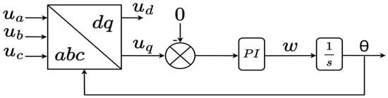
Figure 3.
The control loop of the PLL.
3.2. Design of LCL Filter
The design of the LCL filter plays a critical role in ensuring both harmonic attenuation and system stability in grid-connected voltage source converters (VSCs). In this work, a simplified yet robust methodology was followed, which balances ripple reduction, resonance avoidance, and dynamic performance, while accounting for practical constraints such as low switching frequencies and grid impedance uncertainty. The procedure was adapted from established guidelines in the studies of [7,8,11,78,79,80,81,82,83], and it was refined through analytical derivation and stability checks.
In the s-domain per-phase LCL filtered VSC equivalent circuit seen in Figure 4, the transfer functions are derived as follows:
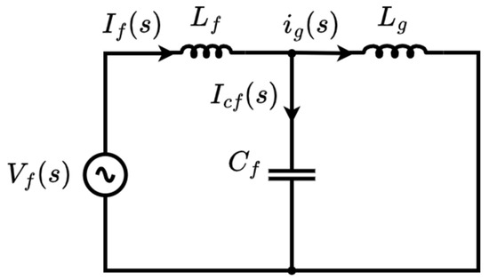
Figure 4.
Per-phase LCL filtered VSC equivalent circuit.
In the s-domain, , , and represent the grid current, the VSC output voltage, and the filter’s capacitor current, respectively. Figure 5 and Figure 6 illustrate the block diagram and the Bode plot according to the transfer function illustrated in (12). At the resonance frequency shown in Figure 6, there is a clear resonance that should be avoided due to the potential for instability caused by the quick phase change. This resonance can be mitigated by applying damping techniques, reducing the sharp peak in magnitude, and smoothing the sudden phase shift.
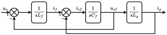
Figure 5.
LCL filter block diagram.

Figure 6.
LCL filter Bode plot.
3.2.1. Filter Design Inputs
The LCL filter design procedure requires the specification of five fundamental system parameters as inputs. These values define the electrical and operational characteristics of the converter-grid interface and serve as the foundation for calculating the filter components. The required inputs are as follows:
- DC-Link Voltage (): This determines the available modulation range and influences the size of the inverter-side inductor.
- Grid Line-to-Line Voltage (): This defines the voltage level that the converter must synchronize with.
- Nominal Grid Frequency (): This affects the resonance conditions and reactive power behavior of the filter capacitor.
- Rated Apparent Power (): This is used to derive the base current and to limit the reactive power drawn by the capacitor.
- Switching Frequency (): This plays a key role in determining the required filter attenuation and the size of the passive components.
3.2.2. Design Objectives and Key Parameters
The primary objectives of the LCL filter design are to achieve effective suppression of switching harmonics, reduce electrical and thermal stress on components, and ensure overall system stability under varying grid conditions. To fulfill these objectives, the LCL filter must be designed in accordance with the following criteria:
- Sufficient attenuation of high-frequency switching harmonics at the converter’s switching frequency.
- Placement of the resonance frequency outside the control bandwidth to avoid excitation.
- Restriction of reactive power drawn by the filter capacitor to prevent degradation of the power factor.
- Minimization of the total inductance to reduce conduction losses and voltage drops.
- Adherence to relevant grid codes concerning THD limits.
To systematically address these criteria, three critical design parameters are utilized:
- Attenuation gain (): Controls the filter’s frequency response and its ability to suppress resonant peaks.
- Current ripple ratio (): Sets an upper limit on the permissible ripple in the converter-side current, influencing the design of the inverter-side inductor.
- Capacitor utilization factor (): Determines the fraction of the maximum allowable filter capacitance to be employed, balancing reactive power and filtering performance.
3.2.3. Filter Capacitor Design ()
The selection of the filter capacitor () in an LCL filter is a critical step that affects both the filtering performance and the power quality at the point of common coupling (PCC). An excessively large capacitor can improve harmonic attenuation but leads to high reactive power injection into the grid, which degrades the system power factor. Conversely, a small capacitor may not provide sufficient attenuation of switching harmonics.
To balance these trade-offs, [78] proposes selecting the capacitor value such that its reactive power consumption at nominal frequency does not exceed 5% of the converter’s rated apparent power. From this, the filter capacitor maximum value ( can be calculated by the following:
To provide flexibility and ensure compliance with practical design constraints, a scaling factor () ∈ [0.5, 1] was introduced. This factor determines the fraction of the maximum allowable filter capacitance that will actually be utilized in the design:
Using a fraction of the maximum allowable capacitance rather than its full value reduces reactive power injection, preserves power factor, and introduces a margin to account for component tolerances and resonance shifts. This approach enables fine-tuning of the filter’s dynamic response, particularly under low switching frequencies.
Due to manufacturing tolerances, the actual value of the filter capacitor may slightly deviate from its nominal value. To account for this, a typical capacitance error of ±5% is considered in the resonance frequency analysis by evaluating both the upper and lower bounds of the capacitance:
3.2.4. Converter-Side Inductance Design ()
The inverter-side inductance () is designed to limit the high-frequency current ripple generated by the PWM switching process. Excessive current ripple not only increases the stress on switching devices and passive components but also degrades current control accuracy. Therefore, a design objective is to ensure that the peak-to-peak current ripple () remains within a specified fraction of the rated current. The ripple is defined as a ratio (Irip) relative to the peak phase current (), typically in the range of 0.05 to 0.25 [82]. Choosing an appropriate value for () allows for a trade-off between ripple suppression and inductor size. The lower ripple values require larger inductors, increasing cost and volume, while higher ripple may compromise performance and increase electromagnetic interference (EMI). Thus, () is selected to meet both electrical and practical design constraints. The maximum current ripple on the converter side, as shown in Figure 7 [78], occurs when the converter voltage falls between to ; thus, it can be expressed as follows:

Figure 7.
The VSC current in relation to the applied VSC voltage.
When the VSC modulation factor (m) is equal to 0.5, the greatest peak-to-peak current ripple happens [79]; then, the expression of (16) can be expressed as follows:
When taking the adequate ripple ratio () from the maximum current (), then the converter side inductance () can be determined from (17), where
3.2.5. Grid-Side Inductance Design
The grid-side inductance was selected to effectively suppress harmonic components in the grid current, ensuring conformity with international standards and utility grid code regulations. After the inverter-side inductance () and filter capacitor () were determined, the grid-side inductance () was calculated to achieve the desired dynamic behavior and place the resonance frequency () within a safe range—away from both the control bandwidth and the switching frequency spectrum. The value of () was derived through the dimensionless parameter (), which reflects the ratio between and , and was directly influenced by the harmonic attenuation rate (). The grid’s injected harmonic current was associated with the one produced by the inverter to be the “harmonic attenuation rate” as in (19) [79]. The typical value to utilize for the harmonic attenuation rate is 20% [80].
From (19), the ratio () can be calculated as follows:
Then
3.2.6. Design Constraints
Resonance Frequency
After choosing the LCL filter’s component values, the resonance frequency should be verified using (22) [11]. To prevent resonance from occurring within the bandwidth of control and to have resonance apparent to the controller, the resonance frequency must adhere to the requirement given by (23) [81].
In systems utilizing PI-based current controllers with grid current feedback, the resonance frequency must be carefully positioned to ensure stable operation. According to [78], stability can be inherently maintained if () falls within a specific frequency window bounded by two critical points: a lower limit ( = ) and an upper limit ( = ). When the resonance frequency resides within this range, the PI controller remains effective, and resonance-related instabilities are avoided.
The grid-side inductance () may vary significantly depending on the grid configuration and connection impedance. Meanwhile, the actual value of the filter capacitor () may deviate slightly from its nominal specification due to manufacturing tolerances, as previously discussed. Since the resonance frequency () is related to both () and (), and the filter inductors () and () are typically fixed by design, the variation range of the resonance frequency can be estimated using Equation (24).
where
Maximum Total Inductance
In LCL filter design, the total inductance () = + must be limited to prevent excessive voltage drop across the filter and to reduce conduction losses. This constraint ensures that the filter inductance remains within 10% of the grid base inductance. High inductance values can degrade dynamic response, increase physical size, and introduce unwanted delays in current control loops. Therefore, an upper bound is imposed on the total inductance to ensure efficient and responsive converter operation. As proposed in the study of [78], the maximum permissible total inductance is given by the following:
The selected filter inductances must satisfy:
Minimum DC-Link Voltage
According to the design procedure in the studies of [78,82], the minimum required DC-link voltage () must ensure that the VSC can supply the maximum required voltage across the filter and the grid under the worst-case conditions. These include the highest possible grid voltage and the voltage drop induced by the current ripple flowing through the total inductance of the LCL filter.
The required condition is derived by evaluating the vector sum of the peak grid voltage () and the maximum voltage drop across the filter inductance (), which occurs at the nominal grid frequency and maximum output current (). The corresponding expression is as follows:
This formulation guarantees that the modulation index of the VSC remains below unity, allowing for sinusoidal voltage generation without entering nonlinear modulation regions. As shown in the study of [78], violating this condition may result in modulation saturation, increased harmonic distortion, or instability, particularly in low switching frequency environments. Therefore, the design must ensure the following:
Harmonic Attenuation Rate (Ka)
A reduced harmonic attenuation rate contributes to diminishing the amplitude of current harmonics, thereby lowering the THD observed in the grid current.
Upon replacing the grid-side inductance with its equivalent expression, the formulas for and were reformulated as follows:
Based on the boundaries according to (24), the corresponding constraints were formulated in the study of [82] as follows:
where
These equations impose a constraint on the harmonic attenuation rate, ensuring that the resulting resonance frequency remains within the stable operating region. Additionally, the selected value of (Ka) must exceed a defined minimum threshold, which corresponds to the maximum allowable resonance shift.
Finally, the design parameter (a) is required to satisfy the following limits:
3.3. Design of Resonance AD Controllers
Since the capacitor causes the resonance, one effective method of AD techniques involves utilizing the current feedback of the LCL filter capacitor with a basic proportional controller to provide compensation. Figure 8 depicts the block diagram of a VSC based on an LCL filter with feedback of the capacitor current. To facilitate the analysis, the capacitor current feedback connection point was moved to the grid current side, producing the block diagram depicted in Figure 9, which produced the same block diagram as Figure 8, except the feedback term will be (). It is feasible to determine the grid current and converter voltage transfer function as follows:
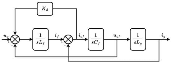
Figure 8.
LCL filter block diagram with the feedback of the capacitor current.

Figure 9.
Equivalent LCL filter block diagram with the feedback of the capacitor current.
It is evident from looking at (12) and (41) that the term appears in the denominator due to the feedback of the capacitor current. The damping factor (ζ) was used to assess the damping intensity [30], which is represented by the following:
where is the angular resonant frequency. Typically, 0.707 is the optimum damping factor based on most of the literature [3,8,12,14,29,30,77]. By implementing (42) on (41), the damping will be achieved if the proper gain is selected as follows:
The Bode plot of (41), shown in Figure 10, when compared to Figure 6, makes it clear how damping techniques can reduce resonance while also mitigating rapid phase shift and peak magnitude reaction.

Figure 10.
LCL filter with AD Bode plot.
3.3.1. GCF
In the practical implementation of active damping strategies, the GCF method is characterized by its simplicity and minimal hardware requirements. This technique employs the measured grid current to generate a damping signal that is fed back to the control loop. The following analysis presents the transfer function derivation and dynamic response evaluation of the GCF configuration.
Figure 11 shows the GCF block diagram, and the transfer function can be derived as in (44). The absence of the second-highest-order term in (44) indicates the difficulty in achieving stability and insufficient damping extent in the case of GCF according to the criteria of (42). The response is therefore dynamically slow, exhibiting a limited control bandwidth. The Bode plot of the transfer function of the GCF is depicted in Figure 12, where it is evident that GCF fails to mitigate the peak magnitude and rapid phase shift.

Figure 11.
The GCF block diagram.
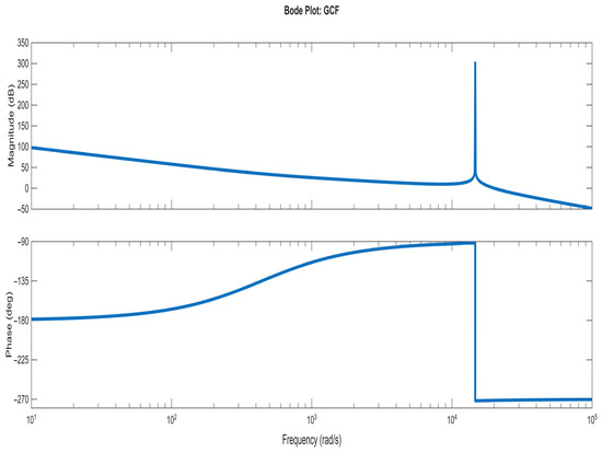
Figure 12.
The Bode plot of GCF.
3.3.2. GCFAD
To enhance the dynamic performance and stability of the GCF approach and to constrain the infinite gain, a practical modification is introduced by incorporating active damping (AD) into the control loop. When adding the AD block as depicted in Figure 13, the transfer function will be as
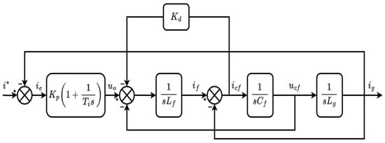
Figure 13.
The GCF with the AD block diagram.
The s3 coefficients in (45) do not contain the current controller parameters ( and ), indicating that the PI controller has no effect on the resonant damping with GCFAD. By implementing (42) on (45), the damping will be achieved as
The Bode plot of the GCFAD transfer function is shown in Figure 14. It clearly demonstrates that the inclusion of active damping significantly attenuates the resonance peak and smooths the phase trajectory. Unlike the undamped GCF response, GCFAD effectively reduces the gain around the resonance frequency, thereby enhancing system stability and preserving phase margin.

Figure 14.
The Bode plot of GCFAD.
3.3.3. CCF
To further investigate the damping capabilities inherent in different feedback strategies, the practical implementation of the CCF technique is analyzed. This subsection presents the restructured block diagram, derivation of the transfer function, and formulation of damping criteria to assess the effectiveness of CCF in suppressing resonance.
To facilitate the analysis, the block diagram of the CCF depicted in Figure 15 is equivalently modified by shifting the feedback current connection point from the converter-current side to the grid-current side. When comparing the CCF block diagram to the GCF, an extra (s2) term appears in the feedback, which is interpreted as the CCF’s inherent damping characteristic [12]. The transfer function of the block diagram depicted in Figure 15 can be obtained as follows:

Figure 15.
The CCF block diagram.
By applying Equation (42) to Equation (47), the damping will be the following:
The Bode plot of the CCF-based control response is illustrated in Figure 16. The inclusion of CCF noticeably reduces the resonance peak and improves phase behavior, indicating inherent damping characteristics. The plot confirms that CCF significantly suppresses the gain at the resonance frequency without the need for additional damping blocks. This inherent damping arises from the feedback path, which includes the filter capacitor and grid inductance, as observed in the block diagram.
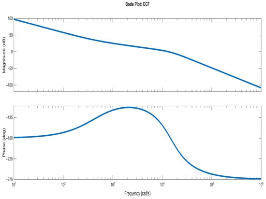
Figure 16.
The Bode plot of CCF.
3.3.4. CCFAD
To enhance the resonance damping performance of the CCF method, especially under conditions where the desired damping ratio cannot be achieved by tuning the proportional gain or the converter-side inductance, an additional damping term can be introduced into the control loop.
When the AD block is added as depicted in Figure 17, the transfer function of CCF will be as follows:
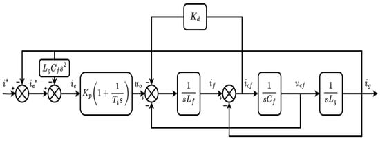
Figure 17.
The CCF with the AD block diagram.
The damping can be reached by:
The Bode plot of the CCFAD transfer function, shown in Figure 18, confirms the successful suppression of the resonance peak and the abrupt phase shift observed in the undamped LCL system. The addition of active damping effectively stabilizes the frequency response and enhances the phase behavior around the resonance region.
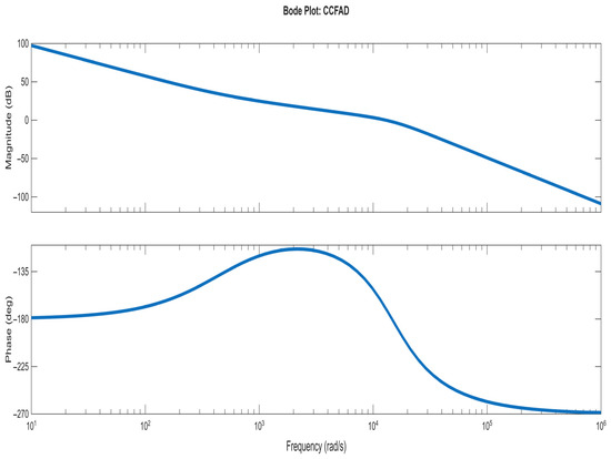
Figure 18.
The Bode plot of CCFAD.
4. Results and Discussion
This section presents a comprehensive evaluation of the system illustrated in Figure 1, considering four control strategies: GCF, GCFAD, CCF, and CCFAD. The assessment combines MATLAB/Simulink-based simulations with real-time validations. Detailed descriptions of the system configuration, including the control parameters and LCL filter component values, are provided in Table 4, Table 5 and Table 6. The performance of the systems was compared in seven different cases:
Table 4.
System parameters.
Table 5.
LCL filter design results.
Table 6.
Controller gains.
- Case 1: Steady-state operating conditions.
- Case 2: Balanced voltage swell.
- Case 3: Balanced voltage sag.
- Case 4: Unbalanced voltage swell.
- Case 5: Unbalanced voltage sag.
- Case 6: Grid frequency drop.
- Case 7: Tracking of active and reactive power (transient analysis).
The selection of these diverse cases was made to thoroughly evaluate the system’s performance under a variety of real-world operational circumstances. The system was tested under voltage sag and swell conditions, as well as balanced and unbalanced grid scenarios, to assess its robustness in the face of both voltage disturbances and grid imbalances. Additionally, a sudden frequency reduction was introduced to evaluate the system’s ability to withstand frequency variations, which may result from sudden changes in loads. The transient tracking of active and reactive powers was conducted to examine dynamic response and control effectiveness, while steady-state testing of harmonics was performed to guarantee the system’s stability and efficiency in situations of continuous load.
All harmonic performance results obtained in this study were benchmarked against the limits defined by the IEEE 519-2022 standard [6] for current harmonics. The evaluation included both total harmonic distortion (THD) and individual harmonic components (e.g., 3rd, 5th, 7th, 9th, and 11th orders), and the compliance of each configuration—namely, CCF, GCFAD, and CCFAD—was explicitly verified in all operating scenarios. Although IEEE 519 recommends using Total Demand Distortion (TDD) for current harmonic assessment, it is common practice—especially in simulations and preliminary studies—to evaluate current harmonics using total harmonic distortion (THD). As highlighted in the study of [84], if compliance with IEEE 519 limits is achieved using THD, then TDD will most likely be within acceptable limits. This approach provides a conservative and valid confirmation of harmonic compliance.
Next, a pole-zero (PZ) map analysis is conducted to assess the closed-loop stability characteristics of each configuration. The results are further validated through real-time implementation using the OPAL-RT platform, with corresponding waveforms and observations compared against simulation outputs. Finally, a sensitivity analysis is performed to quantify the impact of switching frequency on current THD.
The studied system is a three-phase, grid-connected voltage source converter (VSC) rated at 1 MW, operating with a DC-link voltage of 1250 V and interfaced with a 480 V (line-line), 60 Hz grid. The converter is connected to the grid via an LCL filter, whose detailed component values are listed in Table 5. Control is implemented using PI-based current regulators with gains specified in Table 6. Active damping gains are also documented.
All simulations were carried out at a nominal switching frequency of 4800 Hz, unless otherwise specified. For consistency, the following assumptions were made: (i) the AC grid voltage is purely sinusoidal with a fundamental positive-sequence component; (ii) grid impedance is modeled as an ideal short circuit; and (iii) equivalent series resistance (ESR) of passive elements is neglected. These assumptions eliminate passive damping effects, ensuring that all observed damping behavior arises solely from the implemented control strategies.
4.1. Case 1
In this case, the system performance was assessed under normal grid and power reference for four control configurations: GCF, GCFAD, CCF, and CCFAD. The corresponding waveforms for three-phase output voltage, output current, and power at the PCC are presented in Figure 19, while the detailed harmonic analysis, including THD and individual harmonic orders, is summarized in Table 7.
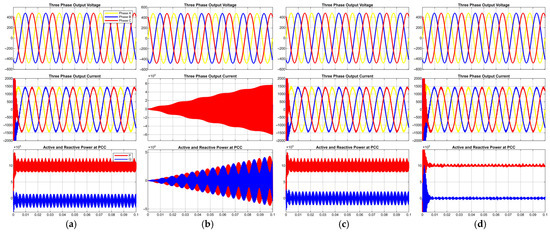
Figure 19.
Output current, output voltage, and injected power in case one: (a) the CCF, (b) the GCF, (c) the CCFAD, (d) the GCFAD.
Table 7.
Harmonic distortion comparison with IEEE 519-2022 under normal conditions.
From the results, it is apparent that the GCF configuration suffers from significant instability. The THD reached 13,971.42%, indicating an unstable and divergent response due to the absence of sufficient damping. This emphasizes that grid current feedback alone is insufficient to maintain stable operation without active damping measures. Accordingly, the GCF configuration will be excluded from further cases, as it failed to achieve stable operation under nominal conditions.
Conversely, the other configurations—GCFAD, CCF, and CCFAD—maintained stable and balanced current injection into the grid. Among these, the harmonic performance of CCFAD remained comparable to that of CCF and GCFAD, with a slightly higher THD of 3.05%, compared to 3.01% and 3.02%, respectively. More importantly, all harmonic components—namely, the 3rd, 5th, 7th, 9th, and 11th—remained well below the limits specified by IEEE 519-2022 [6], confirming full compliance with harmonic standards.
The GCFAD configuration, which incorporates an active damping mechanism into the grid current feedback loop, successfully mitigated the instability observed in the GCF case. As shown in Table 7, the THD was significantly reduced to 3.02%, and all individual harmonic components complied with IEEE 519-2022 limits. This demonstrates that the introduction of active damping is essential to stabilize the system when relying on grid current as the feedback signal. Despite achieving acceptable harmonic performance, the GCFAD approach inherently requires accurate sensing of the grid current and proper tuning of the damping coefficient.
An important observation is the inherent damping capability exhibited by the CCF configuration, which achieved nearly the same performance as the more complex CCFAD. This highlights the effectiveness of converter current feedback in introducing intrinsic damping without requiring additional derivative terms or sensors. In contrast, CCFAD involves increased implementation complexity and sensor requirements due to the inclusion of a derivative action. In cases where the desired damping cannot be achieved by CCF through solely tuning the proportional gain Kp, the CCFAD approach can be adopted as an auxiliary method by introducing additional damping terms to ensure stability.
The waveforms illustrated in Figure 19 further support the numerical findings. In all three stable configurations—GCFAD, CCF, and CCFAD—the output voltage and current exhibit clean, sinusoidal profiles with minimal distortion. The power waveforms at the PCC also confirm stable operation, where the power tracks its reference closely with negligible fluctuations. These results collectively verify that the three damping-based configurations successfully ensure dynamic stability and effective power exchange under normal grid conditions.
4.2. Case 2
In this case, the system was subjected to a high-voltage ride-through (HVRT) scenario, where a sudden voltage swell of 10% was introduced at 0.05 s to evaluate the controller’s robustness and harmonic performance under overvoltage conditions. The three-phase output voltage, current, and PCC power waveforms for the CCF, GCFAD, and CCFAD configurations are illustrated in Figure 20. The corresponding harmonic distortion analysis is provided in Table 8.
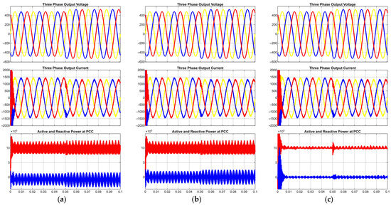
Figure 20.
Output current, output voltage, and injected power in case two: (a) the CCF, (b) the CCFAD, (c) the GCFAD.
Table 8.
Harmonic distortion comparison with IEEE 519-2022 under Case 2.
Despite the voltage swell event, all three control configurations succeeded in maintaining stable operation and balanced current injection. The CCF configuration exhibited the lowest total harmonic distortion (THD) at 3.81%, followed by GCFAD (3.89%) and CCFAD (3.99%). Although the THD values were slightly higher compared to the nominal condition, they remained well within the 5% limit specified by IEEE 519-2022, confirming compliance under overvoltage scenarios.
Examining individual harmonics, the 5th and 7th orders were again the most dominant, with values ranging from 1.51% to 1.80% and 0.85% to 0.96%, respectively. All harmonic components—including the 3rd, 9th, and 11th—remained below their corresponding IEEE 519-2022 limits. Notably, the GCFAD method achieved the lowest 3rd harmonic content at 0.0125%, while CCFAD showed slightly elevated levels in the 11th harmonic (0.3537%), though still acceptable.
The waveform plots In Figure 20 reflect this behavior, with clearly sinusoidal voltage and current profiles and no sign of instability or saturation during the voltage swell. Furthermore, the power at the PCC continued to follow its reference closely with minimal transient deviation, indicating effective control action.
As depicted in Figure 20, both the active and reactive power exhibited transient deviations immediately following the voltage swell disturbance at 0.05 s. The active power showed a bounded overshoot before settling back to its reference value, while the reactive power briefly deviated from zero but promptly returned to its nominal level. Across all configurations, the settling time remained within 90–100 ms, indicating a fast and well-damped dynamic response.
Quantitatively, the GCFAD configuration achieved the lowest active power overshoot at 15.37 kW, compared to 43.44 kW and 43.76 kW for CCF and CCFAD, respectively. The peak active power reached approximately 1.21 MW for GCFAD, while slightly higher peaks of 1.26 MW and 1.27 MW were observed for CCF and CCFAD, respectively.
These findings confirm the ability of the CCF, GCFAD, and CCFAD controllers to withstand short-term voltage swell disturbances while maintaining harmonic compliance and power stability. While CCF exhibited slightly better THD performance, GCFAD outperformed in mitigating specific low-order harmonics and demonstrated the most favorable dynamic behavior.
4.3. Case 3
In this case, the system was exposed to a low-voltage ride-through (LVRT) condition caused by a sudden 10% voltage dip at 0.05 s, simulating a temporary grid disturbance. The objective was to evaluate the controllers’ ability to maintain stability and harmonic compliance during voltage sags. The waveforms of three-phase voltage, current, and PCC power for the CCF, GCFAD, and CCFAD configurations are presented in Figure 21. Table 9 summarizes the harmonic distortion levels for each case.

Figure 21.
Output current, output voltage, and injected power in case three: (a) the CCF, (b) the CCFAD, (c) the GCFAD.
Table 9.
Harmonic distortion comparison with IEEE 519-2022 under Case 3.
All three control configurations demonstrated resilient behavior, sustaining sinusoidal current injection and stable power delivery despite the voltage dip. Among them, the CCF configuration achieved the lowest total harmonic distortion (THD) at 2.24%, followed by CCFAD (2.33%) and GCFAD (2.55%), all well below the IEEE 519-2022 limit of 5%. These results reflect a slight improvement in harmonic performance compared to the voltage swell case (Case 2), indicating favorable conditions for harmonic suppression during undervoltage events.
Regarding individual harmonics, the 5th and 7th orders remained the most dominant across all methods, ranging from 0.71% to 0.79% and 0.48% to 0.51%, respectively, though all remained well below the IEEE 519 thresholds. Notably, CCFAD exhibited the lowest 11th harmonic component at 0.096%, further confirming its effectiveness in suppressing high-order harmonics.
The waveform plots in Figure 21 reveal that all configurations maintained stable voltage and current waveforms with no signs of resonance or distortion growth following the voltage sag. The active and reactive power signals also confirm the system’s dynamic robustness. Both active and reactive power experienced brief transient deviations following the voltage dip at 0.05 s, yet rapidly stabilized thereafter. The active power response showed bounded overshoots of 34.12 kW for CCF, 33.43 kW for CCFAD, and only 18.47 kW for GCFAD, confirming that the latter achieved the most damped transient behavior among the three. Likewise, the peak power reached approximately 1.24 MW (CCF), 1.23 MW (CCFAD), and 1.19 MW (GCFAD), indicating smoother energy exchange with the grid under GCFAD. Across all configurations, the power signals settled within ~100 ms, reflecting a well-damped and fast recovery response.
These findings highlight GCFAD’s advantage in dynamic power stability, while CCFAD offered better suppression of higher-order harmonics, and CCF provided the lowest THD.
4.4. Case 4
In this case, the system was exposed to an unbalanced grid condition by introducing a sudden 20% voltage swell in phase A at 0.05 s. This scenario was designed to assess the controller’s capability to maintain stability and harmonic compliance under asymmetrical voltage disturbances. The voltage, current, and power waveforms for the CCF, GCFAD, and CCFAD configurations are illustrated in Figure 22, while the corresponding harmonic data are provided in Table 10.

Figure 22.
Output current, output voltage, and injected power in case four: (a) the CCF, (b) the CCFAD, (c) the GCFAD.
Table 10.
Harmonic distortion comparison with IEEE 519-2022 under Case 4.
Despite the phase-specific voltage swell, all configurations maintained continuous power injection without entering instability or saturation. However, the harmonic distortion levels increased compared to balanced cases due to the asymmetry of the disturbance. The GCFAD configuration recorded the lowest THD at 4.86%, followed by CCF (4.98%), while CCFAD slightly exceeded the 5% threshold at 5.19%. This suggests that the CCFAD method may require further tuning under unbalanced scenarios to meet IEEE 519-2022 standard limits.
Analyzing the individual harmonic orders reveals that the third, fifth, and seventh harmonics became more prominent due to the imbalance. The third harmonic content, in particular, increased significantly, reaching 3.45% for CCFAD. However, both CCF and GCFAD maintained third harmonic levels just below 3.23% and 3.18%, respectively. The higher harmonics remained within acceptable limits across all methods, although the 11th harmonic under CCFAD reached 0.4033%.
The dynamic behavior of active and reactive power under the unbalanced voltage swell is illustrated in Figure 22. All control configurations responded promptly to the disturbance at 0.05 s, showing transient deviations that were rapidly attenuated. The active power signals exhibited bounded overshoots, with GCFAD achieving the lowest overshoot at only 6.26 kW, compared to 41.77 kW and 43.49 kW for CCFAD and CCF, respectively. This highlights the superior damping capability of GCFAD under asymmetrical voltage conditions. Additionally, the peak power reached 1.08 MW for GCFAD, noticeably lower than the 1.26 MW observed for both CCF and CCFAD, indicating more controlled and conservative energy transfer to the grid.
Overall, GCFAD proved most resilient under unbalanced grid conditions, delivering the lowest THD, best suppression of the third harmonic, and demonstrating the most favorable dynamic performance in terms of overshoot minimization and smooth power recovery. Although CCFAD showed a slight violation of the 5% THD limit, it still ensured system stability and reliable power exchange.
4.5. Case 5
In this case, an imbalanced grid scenario was simulated by introducing a sudden 20% voltage sag in phase A at 0.05 s, aiming to evaluate the controller performance under asymmetrical under-voltage conditions. Figure 23 presents the voltage, current, and PCC power waveforms for the CCF, GCFAD, and CCFAD configurations, while Table 11 lists the corresponding harmonic distortion metrics.

Figure 23.
Output current, output voltage, and injected power in case five: (a) the CCF, (b) the CCFAD and (c) the GCFAD.
Table 11.
Harmonic distortion comparison with IEEE 519-2022 under Case 5.
Despite the asymmetric voltage sag, all controllers sustained power injection without instability or saturation. Among the three methods, GCFAD achieved the lowest THD at 4.41%, followed by CCF (4.47%), while CCFAD recorded the highest value at 4.66%. All configurations remained within the IEEE 519-2022 limit.
The third harmonic was the most dominant due to the unbalance, peaking at 3.93% under CCFAD, while CCF and GCFAD maintained values around 3.71% and 3.64%, respectively. The fifth and seventh harmonic levels remained moderate, with all orders falling well below their limits. CCFAD recorded the highest 11th harmonic at 0.08%, still compliant with the standard.
The dynamic response in terms of active and reactive power is shown in Figure 23. All configurations responded promptly to the sag, with transient power deviations quickly settling within ~100 ms. The active power overshoot was significantly minimized in GCFAD at only 4.61 kW, compared to 34.50 kW and 34.57 kW for CCF and CCFAD, respectively. Moreover, GCFAD reached the lowest peak power at 1.07 MW, indicating better damping and smoother grid interaction under asymmetrical sag conditions.
In summary, GCFAD demonstrated the most robust dynamic behavior with minimal overshoot and peak power and also achieved the lowest THD, reflecting superior overall performance under asymmetrical sag conditions. CCF and CCFAD exhibited slightly higher harmonic levels but still ensured reliable operation and compliance with IEEE 519-2022.
4.6. Case 6
This case examines the system’s behavior under a grid frequency disturbance, simulated by a sudden drop from 60 Hz to 59.76 Hz at 0.05 s. The objective was to evaluate the impact of frequency deviations on the controller performance in terms of harmonic quality and power stability. The waveforms of the output voltage, current, and PCC power for the CCF, GCFAD, and CCFAD controllers are illustrated in Figure 24, and the corresponding harmonic data are presented in Table 12.
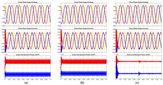
Figure 24.
Output current, output voltage, and injected power in case six: (a) the CCF, (b) the CCFAD, (c) the GCFAD.
Table 12.
Harmonic distortion comparison with IEEE 519-2022 under Case 6.
All control configurations maintained stable current injection and consistent power delivery, indicating resilience against minor frequency variations. The total harmonic distortion (THD) values remained low and within IEEE 519-2022 limits for all methods, with CCF achieving the lowest THD at 3.01%, followed closely by CCFAD (3.04%) and GCFAD (3.05%).
In terms of individual harmonics, the fifth and seventh orders were the most dominant, yet all remained well below the standard thresholds. The third harmonic component was effectively minimized by GCFAD at 0.0566%, compared to 0.1335% and 0.1029% for CCF and CCFAD, respectively. Similarly, the 11th harmonic was also lowest under GCFAD.
Regarding dynamic performance, all controllers quickly responded to the frequency drop at 0.05 s, with transient effects dissipating rapidly. The active power overshoot was significantly reduced under GCFAD at only 8.50 kW, compared to 38.19 kW and 37.75 kW for CCF and CCFAD, respectively. Furthermore, the peak power for GCFAD was limited to 1.11 MW, which is lower than the 1.23 MW and 1.24 MW recorded for CCF and CCFAD, respectively.
Overall, GCFAD delivered the best dynamic performance, in terms of overshoot and peak power minimization, and also showed excellent harmonic suppression, particularly for the 3rd and 11th harmonics. While CCF slightly outperformed others in THD, the differences were marginal, and all methods ensured reliable operation under frequency deviations.
4.7. Case 7
Figure 25 presents the transient response of the system under sequential step changes in active and reactive power references. The active power reference was raised from 0 to 1 MW at 0.02 s and returned to 0 MW at 0.06 s, while the reactive power reference was increased from 0 to 1 MVAR at 0.04 s and set back to 0 MVAR at 0.08 s. This test aimed to assess the controllers’ ability to follow dynamic power demands with minimal distortion and stable operation.
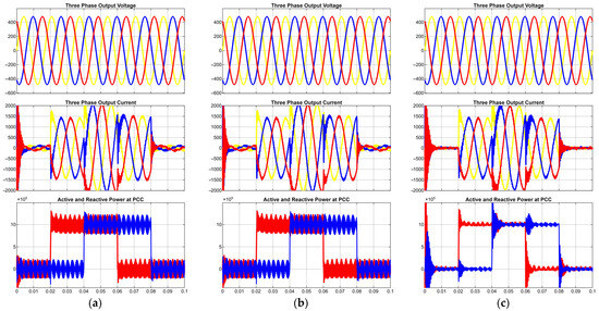
Figure 25.
Output current, output voltage, and injected power in case seven: (a) the CCF, (b) the CCFAD, (c) the GCFAD.
All controllers—CCF, GCFAD, and CCFAD—successfully tracked the reference signals without loss of synchronism or instability. However, the GCFAD configuration exhibited noticeable overshoot, particularly during the initial step in active power, and demonstrated limited decoupling between the active and reactive power. In contrast, both CCF and CCFAD showed well-damped responses and maintained better decoupling between the power components during transitions.
4.8. Stability Analysis
To assess the stability characteristics of the studied current control strategies, a detailed pole-zero map (PZ map) analysis was conducted for the closed-loop transfer functions corresponding to GCF, GCFAD, CCF, and CCFAD. The corresponding PZ map is illustrated in Figure 26, and its numerical values are summarized in Table 13.
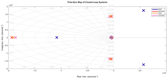
Figure 26.
Closed-loop pole-zero map for compared controllers.
Table 13.
Poles, zeros, and stability of closed-loop systems.
In the GCF structure, grid current feedback introduces a real zero at approximately −439.6 and a pole at −451, in addition to a complex conjugate pole pair at 5637 + j17468 and 5637 − j17468, and a real pole at −10822. It is worth noting that the complex conjugate poles lie in the right-half plane (RHP), indicating the presence of unstable dynamics. Despite the implementation of current feedback, the dominant poles remain on the right side of the imaginary axis, and, thus, the closed-loop system is classified as unstable.
The inclusion of active damping in GCFAD significantly improves system stability. The poles shift deeper into the left-half plane (LHP), with one real dominant pole at −19380, a complex conjugate pair at −444 + j13717 and −444 − j13717, and an additional pole at −451. Zeros are located at −451 and −439.6. This leftward pole shift indicates increased damping of resonant components and confirms stability.
Similarly, the CCF controller exhibits an improved pole configuration, with a dominant real pole at –19048 and a complex pair at −610 + j13822 and −610 − j13822, accompanied by a zero at −439.6. Further improvement is achieved with the CCFAD scheme, where the poles shift to −18677 and −783 + j13577, −783 − j13577, with corresponding zeros at −476 and −462.7. The more pronounced displacement of poles to the left suggests a stronger damping effect and enhanced system robustness.
In summary, the stability analysis confirms that both GCFAD and CCFAD techniques effectively stabilize the system, with CCFAD demonstrating comparatively superior damping due to deeper pole placement. On the other hand, the GCF system, in the absence of active damping, remains unstable.
4.9. Real-Time Validations
To further validate the findings obtained from the MATLAB/Simulink simulations, real-time testing was conducted using the OPAL-RT OP4510 platform. The same test case (Case 1) and control configurations—GCF, GCFAD, CCF, and CCFAD—were implemented and evaluated.
The Simulink-based control model was compiled into a real-time executable and deployed onto the OPAL-RT hardware platform, as shown in Figure 27. This enabled the system to operate under real-time constraints, providing a realistic validation environment that closely emulates the dynamic behavior of the physical system.
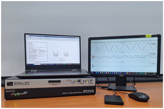
Figure 27.
Real-time validation setup using OPAL-RT.
The real-time waveforms for each configuration are presented in Figure 28, Figure 29, Figure 30 and Figure 31, while the corresponding MATLAB/Simulink-based simulation results are shown in Figure 19. Upon comparison, the real-time results closely matched the simulation outcomes. In both environments, the GCF configuration exhibited clear instability and failed to maintain bounded current and power profiles. Conversely, the damping-based schemes—GCFAD, CCF, and CCFAD—produced sinusoidal waveforms and ensured stable operation, confirming the effectiveness of the proposed control strategies.
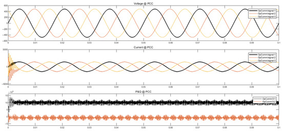
Figure 28.
The CCF output current, output voltage, and injected power in case one using OPAL-RT.

Figure 29.
The GCF output current, output voltage, and injected power in case one using OPAL-RT.

Figure 30.
The CCFAD output current, output voltage, and injected power in case one using OPAL-RT.
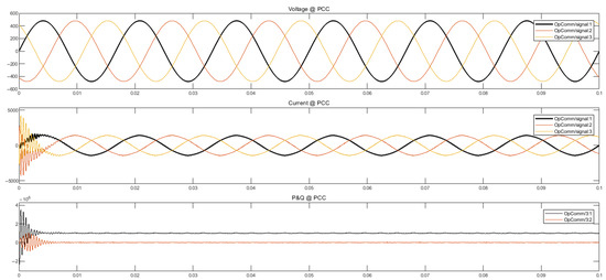
Figure 31.
The GCFAD output current, output voltage, and injected power in case one using OPAL-RT.
Minor differences in signal amplitude and transient settling time were observed in the OPAL-RT results. However, these discrepancies did not affect the overall system behavior or control performance, thereby reinforcing the credibility and robustness of the simulation-based conclusions.
4.10. Sensitivity Analysis of Switching Frequency
To investigate the impact of switching frequency on the harmonic performance of the current injected into the grid, a dedicated sensitivity analysis was performed. The THD was evaluated for three control configurations—CCF, GCFAD, and CCFAD—while varying the switching frequency fs from 2800 Hz to 10,800 Hz. The results are tabulated in Table 14 and graphically illustrated in Figure 32. This analysis was conducted under the following assumptions and constraints:
Table 14.
Switching frequency sensitivity test results.
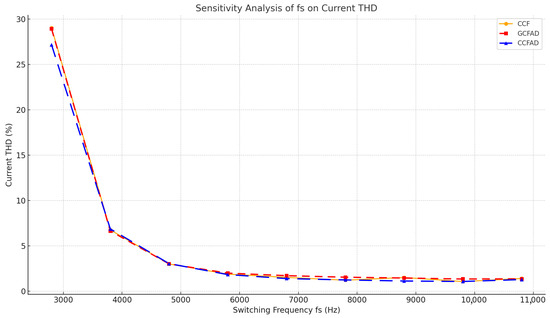
Figure 32.
Variation in current THD with switching frequency for CCF, GCFAD, and CCFAD configurations.
- The system parameters were designed and fixed based on a nominal switching frequency of 4800 Hz.
- No equivalent series resistance (ESR) or additional passive damping was included in the LCL filter, effectively eliminating internal damping effects and exposing the system to ideal resonance behavior.
- The grid was modeled as an ideal source with purely positive-sequence components and zero source impedance.
From the results, it is evident that the THD is significantly influenced by the selected switching frequency. As shown in Table 14, low switching frequencies (e.g., 2800 Hz) result in extremely high THD values exceeding 27% for all schemes, rendering the system unstable or non-compliant with harmonic standards.
In contrast, increasing fs leads to a sharp reduction in THD, with all configurations achieving THD < 5% for fs > 3800 Hz. The lowest THD values are observed around 7800–9800 Hz. However, it is notable that, beyond this point, the THD does not improve significantly and may exhibit slight fluctuations due to switching artifacts, as evident in the increase at 10,800 Hz.
High switching frequencies offer the advantages of enhanced harmonic attenuation and reduced LCL filter size; however, they come at the expense of increased switching losses and elevated thermal stress.
Overall, this analysis confirms that 4800 Hz–7800 Hz represents a practical and efficient operating range for the studied 1 MW grid-tied converter, balancing harmonic compliance and switching loss considerations.
5. Conclusions
This paper presented a comprehensive analysis and performance comparison of four current control strategies for three-phase grid-connected VSCs with LCL filters: GCF, GCFAD, CCF, and CCFAD. This study focused on low switching frequency operation and covered LCL filter design, controller modeling, closed-loop stability assessment using pole-zero analysis, harmonic and dynamic performance evaluation under multiple operating scenarios, and real-time validations using OPAL-RT.
The results demonstrated that, while the GCF approach lacks adequate damping and results in instability, both GCFAD and CCFAD significantly improve system stability and harmonic compliance. Notably, the CCF configuration—despite its simplicity—exhibited inherent damping and achieved competitive performance compared to more complex active damping schemes. Moreover, real-time experimental results aligned closely with simulation data, reinforcing the practical applicability of the proposed strategies. Sensitivity analysis on switching frequency further confirmed the critical role of proper selection of switching frequency in maintaining THD within grid code limits.
A summary comparison of the four controllers in terms of complexity, dynamic response, stability, and harmonic ranking across test cases is provided in Table 15.
Table 15.
Performance comparison of the four current controllers.
Future work will aim to evaluate the proposed strategies under variable grid impedance conditions, extend their functionality to support grid-forming and islanding modes, and incorporate adaptive or intelligent control techniques (e.g., Fuzzy Logic, ANN, or MPC) to enhance system robustness.
Author Contributions
Conceptualization, M.A. and A.A.A.; methodology, M.A., A.A.A. and F.H.; software, M.A. and A.A.A.; validation, M.A. and A.A.A.; formal analysis, M.A., A.A.A. and S.A.; investigation, M.A., A.A.A. and F.H.; resources, S.A. and Y.A.A.; data curation, S.A. and Y.A.A.; writing—original draft preparation, M.A., A.A.A. and F.H.; writing—review and editing, M.A., S.A. and Y.A.A.; visualization, F.H., S.A. and Y.A.A.; supervision, Y.A.A.; project administration, A.A.A. and Y.A.A.; funding acquisition, Y.A.A. All authors have read and agreed to the published version of the manuscript.
Funding
This research work was funded by the Institutional Fund Projects under grant no. (IFPDP-240-22).
Data Availability Statement
All data required are provided within this manuscript.
Acknowledgments
This research work was funded by the Institutional Fund Projects under grant no. (IFPDP-240-22). Therefore, the authors gratefully acknowledge technical and financial support from the Ministry of Education and Deanship of Scientific Research (DSR), King Abdulaziz University (KAU), Jeddah, Saudi Arabia.
Conflicts of Interest
The authors declare no conflicts of interest.
Abbreviations
The following abbreviations are used in this manuscript:
| AD | Active Damping |
| CCF | Converter Current Feedback |
| CCFAD | Converter Current Feedback with Active Damping (Capacitor Current Feedback) |
| DG | Distributed Generation |
| GCF | Grid Current Feedback |
| GCFAD | Grid Current Feedback with Active Damping (Capacitor Current Feedback) |
| L | Inductor (or L Filter) |
| LC | Inductor–Capacitor Filter |
| LCL | Inductor–Capacitor–Inductor Filter |
| PD | Passive Damping |
| PI | Proportional–Integral (Controller) |
| PLL | Phase-Locked Loop |
| PWM | Pulse Width Modulation |
| THD | Total Harmonic Distortion |
| VSC | Voltage Source Converter |
References
- Almatani, N.O.; Alhussainy, A.A.; Alghamdi, S.; Kotb, H.; AboRas, K.M.; Vellingiri, M.; Rawa, M. Assessment of a High-Order Stationary Frame Controller for Two-Level and Three-Level NPC Grid-Connected Inverters. Energies 2022, 15, 9313. [Google Scholar] [CrossRef]
- Ma, W.; Guan, Y.; Zhang, B.; Wu, L. Active Disturbance Rejection Control Based Single Current Feedback Resonance Damping Strategy for LCL-Type Grid-Connected Inverter. IEEE Trans. Energy Convers. 2021, 36, 48–62. [Google Scholar] [CrossRef]
- Ruan, X.; Wang, X.; Pan, D.; Yang, D.; Li, W.; Bao, C. Control Techniques for LCL-Type Grid-Connected Inverters; CPSS Power Electronics Series; Springer: Singapore, 2018; ISBN 978-981-10-4276-8. [Google Scholar]
- Sosa, J.M.; Escobar, G.; Martínez-Rodríguez, P.R.; Vázquez, G.; Juárez, M.A.; Diosdado, M. Comparative Evaluation of L and LCL Filters in Transformerless Grid Tied Converters for Active Power Injection. In Proceedings of the 2014 IEEE International Autumn Meeting on Power, Electronics and Computing (ROPEC), Ixtapa, Mexico, 5–7 November 2014; pp. 1–6. [Google Scholar]
- Lettl, J.; Bauer, J.; Linhart, L. Comparison of Different Filter Types for Grid Connected Inverter. In Proceedings of the PIERS Proceedings, Marrakesh, Morocco, 20–23 March 2011. [Google Scholar]
- IEEE Std 519-2022 Revis. IEEE Std 519-2014; IEEE Standard for Harmonic Control in Electric Power Systems. IEEE: New York, NY, USA, 2022; pp. 1–31. [CrossRef]
- IEEE Std 1547-2003; IEEE Standard for Interconnecting Distributed Resources with Electric Power Systems. IEEE: New York, NY, USA, 2003; pp. 1–28. [CrossRef]
- Yagnik, U.P.; Solanki, M.D. Comparison of L, LC & LCL Filter for Grid Connected Converter. In Proceedings of the 2017 International Conference on Trends in Electronics and Informatics (ICEI), Tirunelveli, India, 11–12 May 2017; pp. 455–458. [Google Scholar]
- Elsaharty, M.A.; Ashour, H.A. Passive L and LCL Filter Design Method for Grid-Connected Inverters. In Proceedings of the 2014 IEEE Innovative Smart Grid Technologies—Asia (ISGT ASIA), Kuala Lumpur, Malaysia, 20–23 May 2014; pp. 13–18. [Google Scholar]
- Wu, W.; Liu, Y.; He, Y.; Chung, H.S.-H.; Liserre, M.; Blaabjerg, F. Damping Methods for Resonances Caused by LCL-Filter-Based Current-Controlled Grid-Tied Power Inverters: An Overview. IEEE Trans. Ind. Electron. 2017, 64, 7402–7413. [Google Scholar] [CrossRef]
- Peña-Alzola, R.; Liserre, M.; Blaabjerg, F.; Ordonez, M.; Yang, Y. LCL-Filter Design for Robust Active Damping in Grid-Connected Converters. IEEE Trans. Ind. Inform. 2014, 10, 2192–2203. [Google Scholar] [CrossRef]
- Tang, Y.; Loh, P.C.; Wang, P.; Choo, F.H.; Gao, F. Exploring Inherent Damping Characteristic of LCL-Filters for Three-Phase Grid-Connected Voltage Source Inverters. IEEE Trans. Power Electron. 2012, 27, 1433–1443. [Google Scholar] [CrossRef]
- Pan, D.; Ruan, X.; Wang, X.; Bao, C.; Li, W. Robust Capacitor-Current-Feedback Active Damping for the LCL-Type Grid-Connected Inverter. In Proceedings of the 2013 IEEE Energy Conversion Congress and Exposition, Denver, CO, USA, 15–19 September 2013; pp. 728–735. [Google Scholar]
- Xu, J.; Xie, S.; Tang, T. Active Damping-Based Control for Grid-Connected LCL-Filtered Inverter With Injected Grid Current Feedback Only. IEEE Trans. Ind. Electron. 2014, 61, 4746–4758. [Google Scholar] [CrossRef]
- Zhang, C.; Dragicevic, T.; Vasquez, J.C.; Guerrero, J.M. Resonance Damping Techniques for Grid-Connected Voltage Source Converters with LCL Filters—A Review. In Proceedings of the 2014 IEEE International Energy Conference (ENERGYCON), Dubrovnik, Croatia, 13–16 May 2014; pp. 169–176. [Google Scholar]
- Xu, J.; Xie, S. LCL-Resonance Damping Strategies for Grid-Connected Inverters with LCL Filters: A Comprehensive Review. J. Mod. Power Syst. Clean Energy 2018, 6, 292–305. [Google Scholar] [CrossRef]
- Dannehl, J.; Liserre, M.; Fuchs, F.W. Filter-Based Active Damping of Voltage Source Converters With LCL Filter. IEEE Trans. Ind. Electron. 2011, 58, 3623–3633. [Google Scholar] [CrossRef]
- Zhao, W.; Chen, G. Comparison of Active and Passive Damping Methods for Application in High Power Active Power Filter with LCL-Filter. In Proceedings of the 2009 International Conference on Sustainable Power Generation and Supply, Nanjing, China, 6–7 April 2009; pp. 1–6. [Google Scholar]
- He, N.; Xu, D.; Zhu, Y.; Zhang, J.; Shen, G.; Zhang, Y.; Ma, J.; Liu, C. Weighted Average Current Control in a Three-Phase Grid Inverter With an LCL Filter. IEEE Trans. Power Electron. 2013, 28, 2785–2797. [Google Scholar] [CrossRef]
- Dannehl, J.; Fuchs, F.W.; Hansen, S.; Thøgersen, P.B. Investigation of Active Damping Approaches for PI-Based Current Control of Grid-Connected Pulse Width Modulation Converters With LCL Filters. IEEE Trans. Ind. Appl. 2010, 46, 1509–1517. [Google Scholar] [CrossRef]
- Bao, C.; Ruan, X.; Wang, X.; Li, W.; Pan, D.; Weng, K. Step-by-Step Controller Design for LCL-Type Grid-Connected Inverter with Capacitor–Current-Feedback Active-Damping. IEEE Trans. Power Electron. 2014, 29, 1239–1253. [Google Scholar] [CrossRef]
- Ma, Z.; Zhou, L.; Liu, J. Proportional Capacitor Current Feedback Based Active Damping Control for LCL-Filter Converters with Considerable Control Delay. In Proceedings of the 2020 IEEE Applied Power Electronics Conference and Exposition (APEC), New Orleans, LA, USA, 15–19 March 2020; pp. 3110–3114. [Google Scholar]
- Li, X.; Wu, X.; Geng, Y.; Yuan, X.; Xia, C.; Zhang, X. Wide Damping Region for LCL-Type Grid-Connected Inverter With an Improved Capacitor-Current-Feedback Method. IEEE Trans. Power Electron. 2015, 30, 5247–5259. [Google Scholar] [CrossRef]
- Wang, X.; Blaabjerg, F.; Loh, P.C. Grid-Current-Feedback Active Damping for LCL Resonance in Grid-Connected Voltage-Source Converters. IEEE Trans. Power Electron. 2016, 31, 213–223. [Google Scholar] [CrossRef]
- Wang, X.; Blaabjerg, F.; Loh, P.C. Analysis and Design of Grid-Current-Feedback Active Damping for LCL Resonance in Grid-Connected Voltage Source Converters. In Proceedings of the 2014 IEEE Energy Conversion Congress and Exposition (ECCE), Pittsburgh, PA, USA, 14–18 September 2014; pp. 373–380. [Google Scholar]
- Wu, E.; Lehn, P.W. Digital Current Control of a Voltage Source Converter with Active Damping of LCL Resonance. In Proceedings of the Twentieth Annual IEEE Applied Power Electronics Conference and Exposition, APEC 2005, Austin, TX, USA, 6–10 March 2005; Volume 3, pp. 1642–1649. [Google Scholar]
- Dannehl, J.; Fuchs, F.W.; Thøgersen, P.B. PI State Space Current Control of Grid-Connected PWM Converters With LCL Filters. IEEE Trans. Power Electron. 2010, 25, 2320–2330. [Google Scholar] [CrossRef]
- Massing, J.R.; Stefanello, M.; Grundling, H.A.; Pinheiro, H. Adaptive Current Control for Grid-Connected Converters With LCL Filter. IEEE Trans. Ind. Electron. 2012, 59, 4681–4693. [Google Scholar] [CrossRef]
- Frede, B. Control of Power Electronic Converters and Systems; Academic Press: Cambridge, UK, 2021; Volume 3, ISBN 978-0-12-819432-4. [Google Scholar]
- Matijevic, E.; Sharma, R.; Zare, F.; Kumar, D. A Unified Active Damping for Grid and Converter Current Feedback in Active Front End Converters. IEEE Access 2022, 10, 30913–30924. [Google Scholar] [CrossRef]
- Edpuganti, A.; Rathore, A.K. A Survey of Low Switching Frequency Modulation Techniques for Medium-Voltage Multilevel Converters. IEEE Trans. Ind. Appl. 2015, 51, 4212–4228. [Google Scholar] [CrossRef]
- Wang, Z.; Hao, S.; Han, D.; Jin, X.; Gu, X. Low Switching Frequency Operation Control of Line Voltage Cascade Triple Converter. Electronics 2021, 10, 3059. [Google Scholar] [CrossRef]
- Roldan-Perez, J.; Avila-Martinez, R.; Rodriguez-Cabero, A.; Prodanovic, M.; Bueno, E. LTCL-Filter Active-Damping Design Considerations for Low-Switching-Frequency Grid-Tied VSCs. In Proceedings of the IECON 2018—44th Annual Conference of the IEEE Industrial Electronics Society, Washington, DC, USA, 21–23 October 2018; IEEE: New York, NY, USA, 2018; pp. 1315–1320. [Google Scholar]
- Ricchiuto, D.; Liserre, M.; De Santis, D. Low-Switching-Frequency Active Damping Methods of Medium-Voltage Multilevel Inverters. In Proceedings of the 2012 IEEE International Symposium on Industrial Electronics, Hangzhou, China, 28–31 May 2012; IEEE: New York, NY, USA, 2012; pp. 1991–1996. [Google Scholar]
- Xu, A.J.; Xie, B.S.; Kan, C.J.; Ji, D.L. An Improved Inverter-Side Current Feedback Control for Grid-Connected Inverters with LCL Filters. In Proceedings of the 2015 9th International Conference on Power Electronics and ECCE Asia (ICPE-ECCE Asia), Seoul, Republic of Korea, 1–5 June 2015; IEEE: New York, NY, USA, 2015; pp. 984–989. [Google Scholar]
- Liu, Z.; Liu, J.J.; Zhao, Y.L. A Unified Control Strategy for Three-Phase Inverter in Distributed Generation. IEEE Trans. Power Electron. 2014, 29, 1176–1191. [Google Scholar] [CrossRef]
- Miret, J.; Camacho, A.; Castilla, M.; De Vicuna, L.G.; Matas, J. Control Scheme With Voltage Support Capability for Distributed Generation Inverters Under Voltage Sags. IEEE Trans. Power Electron. 2013, 28, 5252–5262. [Google Scholar] [CrossRef]
- Li, Y.; Jiang, S.; Cintron-Rivera, J.G.; Peng, F.Z. Modeling and Control of Quasi-Z-Source Inverter for Distributed Generation Applications. IEEE Trans. Ind. Electron. 2013, 60, 1532–1541. [Google Scholar] [CrossRef]
- Selvaraj, J.; Rahim, N.A. Multilevel Inverter For Grid-Connected PV System Employing Digital PI Controller. IEEE Trans. Ind. Electron. 2009, 56, 149–158. [Google Scholar] [CrossRef]
- Yuan, X.; Merk, W.; Stemmler, H.; Allmeling, J. Stationary-Frame Generalized Integrators for Current Control of Active Power Filters with Zero Steady-State Error for Current Harmonics of Concern under Unbalanced and Distorted Operating Conditions. IEEE Trans. Ind. Appl. 2002, 38, 523–532. [Google Scholar] [CrossRef]
- Freijedo, F.D.; Vidal, A.; Yepes, A.G.; Guerrero, J.M.; Lopez, O.; Malvar, J.; Doval-Gandoy, J. Tuning of Synchronous-Frame PI Current Controllers in Grid-Connected Converters Operating at a Low Sampling Rate by MIMO Root Locus. IEEE Trans. Ind. Electron. 2015, 62, 5006–5017. [Google Scholar] [CrossRef]
- Dai, M.; Marwali, M.N.; Jung, J.-W.; Keyhani, A. A Three-Phase Four-Wire Inverter Control Technique for a Single Distributed Generation Unit in Island Mode. IEEE Trans. Power Electron. 2008, 23, 322–331. [Google Scholar] [CrossRef]
- Castilla, M.; Miret, J.; Matas, J.; Garcia De Vicuna, L.; Guerrero, J.M. Control Design Guidelines for Single-Phase Grid-Connected Photovoltaic Inverters With Damped Resonant Harmonic Compensators. IEEE Trans. Ind. Electron. 2009, 56, 4492–4501. [Google Scholar] [CrossRef]
- Jia, Y.Q.; Zhao, J.Q.; Fu, X.W. Direct Grid Current Control of LCL-Filtered Grid-Connected Inverter Mitigating Grid Voltage Disturbance. IEEE Trans. Power Electron. 2014, 29, 1532–1541. [Google Scholar] [CrossRef]
- Delghavi, M.B.; Yazdani, A. Islanded-Mode Control of Electronically Coupled Distributed-Resource Units Under Unbalanced and Nonlinear Load Conditions. IEEE Trans. Power Deliv. 2011, 26, 661–673. [Google Scholar] [CrossRef]
- Holmes, D.G.; Lipo, T.A.; McGrath, B.P.; Kong, W.Y. Optimized Design of Stationary Frame Three Phase AC Current Regulators. IEEE Trans. Power Electron. 2009, 24, 2417–2426. [Google Scholar] [CrossRef]
- Ye, H.; Pei, W.; Kong, L.; An, T. Low-Order Response Modeling for Wind Farm-MTDC Participating in Primary Frequency Controls. IEEE Trans. Power Syst. 2019, 34, 942–952. [Google Scholar] [CrossRef]
- Markovic, U.; Chu, Z.; Aristidou, P.; Hug, G. LQR-Based Adaptive Virtual Synchronous Machine for Power Systems With High Inverter Penetration. IEEE Trans. Sustain. Energy 2019, 10, 1501–1512. [Google Scholar] [CrossRef]
- Olalla, C.; Leyva, R.; El Aroudi, A.; Queinnec, I. Robust LQR Control for PWM Converters: An LMI Approach. IEEE Trans. Ind. Electron. 2009, 56, 2548–2558. [Google Scholar] [CrossRef]
- Mohseni, M.; Islam, S.M. A New Vector-Based Hysteresis Current Control Scheme for Three-Phase PWM Voltage-Source Inverters. IEEE Trans. Power Electron. 2010, 25, 2299–2309. [Google Scholar] [CrossRef]
- Prabhakar, N.; Mishra, M.K. Dynamic Hysteresis Current Control to Minimize Switching for Three-Phase Four-Leg VSI Topology to Compensate Nonlinear Load. IEEE Trans. Power Electron. 2010, 25, 1935–1942. [Google Scholar] [CrossRef]
- Shukla, A.; Ghosh, A.; Joshi, A. Hysteresis Modulation of Multilevel Inverters. IEEE Trans. Power Electron. 2011, 26, 1396–1409. [Google Scholar] [CrossRef]
- Zhang, Y.; Li, Z.; Zhang, Y.; Xie, W.; Piao, Z.; Hu, C. Performance Improvement of Direct Power Control of PWM Rectifier With Simple Calculation. IEEE Trans. Power Electron. 2013, 28, 3428–3437. [Google Scholar] [CrossRef]
- Mir, A.S.; Senroy, N. Adaptive Model Predictive Control Scheme for Application of SMES for Load Frequency Control. IEEE Trans. Power Syst. 2024, 1. [Google Scholar] [CrossRef]
- Hu, J.; Nian, H.; Hu, B.; He, Y.; Zhu, Z.Q. Direct Active and Reactive Power Regulation of DFIG Using Sliding-Mode Control Approach. IEEE Trans. Energy Convers. 2010, 25, 1028–1039. [Google Scholar] [CrossRef]
- Mohamed, Y.A.-R.I. Mitigation of Converter-Grid Resonance, Grid-Induced Distortion, and Parametric Instabilities in Converter-Based Distributed Generation. IEEE Trans. Power Electron. 2011, 26, 983–996. [Google Scholar] [CrossRef]
- Azeem, H.; Yellasiri, S.; Jammala, V.; Naik, B.S.; Panda, A.K. A Fuzzy Logic Based Switching Methodology for a Cascaded H-Bridge Multi-Level Inverter. IEEE Trans. Power Electron. 2019, 34, 9360–9364. [Google Scholar] [CrossRef]
- Talaq, J.; Al-Basri, F. Adaptive Fuzzy Gain Scheduling for Load Frequency Control. IEEE Trans. Power Syst. 1999, 14, 145–150. [Google Scholar] [CrossRef]
- Wang, H.; Li, Z.S. Multi-Area Load Frequency Control in Power System Integrated With Wind Farms Using Fuzzy Generalized Predictive Control Method. IEEE Trans. Reliab. 2023, 72, 737–747. [Google Scholar] [CrossRef]
- Aziz, S.; Wang, H.; Liu, Y.; Peng, J.; Jiang, H. Variable Universe Fuzzy Logic-Based Hybrid LFC Control With Real-Time Implementation. IEEE Access 2019, 7, 25535–25546. [Google Scholar] [CrossRef]
- Zhang, C.; Mijatovic, N.; Cai, X.; Dragicevic, T. Artificial Neural Network-Based Pole-Tracking Method for Online Stabilization Control of Grid-Tied VSC. IEEE Trans. Ind. Electron. 2022, 69, 13902–13909. [Google Scholar] [CrossRef]
- Xu, J.; Wu, Z.; Yang, X.; Ye, J.; Shen, A. ANN-Based Control Method Implemented in a Voltage Source Converter for Industrial Micro-Grid. In Proceedings of the 2011 Sixth International Conference on Bio-Inspired Computing: Theories and Applications, Penang, Malaysia, 27–29 September 2011; IEEE: New York, NY, USA, 2011; pp. 140–145. [Google Scholar]
- Al-Majidi, S.D.; Al-Nussairi, M.K.; Mohammed, A.J.; Dakhil, A.M.; Abbod, M.F.; Al-Raweshidy, H.S. Design of a Load Frequency Controller Based on an Optimal Neural Network. Energies 2022, 15, 6223. [Google Scholar] [CrossRef]
- Kang, J.; Meng, W.; Abraham, A.; Liu, H. An Adaptive PID Neural Network for Complex Nonlinear System Control. Neurocomputing 2014, 135, 79–85. [Google Scholar] [CrossRef]
- Choi, D.-K.; Lee, K.-B. Dynamic Performance Improvement of AC/DC Converter Using Model Predictive Direct Power Control With Finite Control Set. IEEE Trans. Ind. Electron. 2015, 62, 757–767. [Google Scholar] [CrossRef]
- Mariethoz, S.; Morari, M. Explicit Model-Predictive Control of a PWM Inverter With an LCL Filter. IEEE Trans. Ind. Electron. 2009, 56, 389–399. [Google Scholar] [CrossRef]
- Liu, J.; Yao, Q.; Hu, Y. Model Predictive Control for Load Frequency of Hybrid Power System with Wind Power and Thermal Power. Energy 2019, 172, 555–565. [Google Scholar] [CrossRef]
- Cortes, P.; Kazmierkowski, M.P.; Kennel, R.M.; Quevedo, D.E.; Rodriguez, J. Predictive Control in Power Electronics and Drives. IEEE Trans. Ind. Electron. 2008, 55, 4312–4324. [Google Scholar] [CrossRef]
- Fu, C.; Liu, J.; Zhang, Z.; Wang, Q.-G.; Yu, J. Cascade Finite-Time Adaptive Control for Stand-Alone Inverters With Load Disturbances. IEEE Trans. Autom. Sci. Eng. 2025, 22, 16512–16521. [Google Scholar] [CrossRef]
- Nazir, R.; Wood, A.; Laird, H.; Watson, N. An Adaptive Repetitive Controller for Three-Phase PWM Regenerative Rectifiers. In Proceedings of the 2015 International Conference on Renewable Energy Research and Applications (ICRERA), Palermo, Italy, 22–25 November 2015; IEEE: New York, NY, USA, 2015; pp. 1126–1131. [Google Scholar]
- Do, T.D.; Leu, V.Q.; Choi, Y.-S.; Choi, H.H.; Jung, J.-W. An Adaptive Voltage Control Strategy of Three-Phase Inverter for Stand-Alone Distributed Generation Systems. IEEE Trans. Ind. Electron. 2013, 60, 5660–5672. [Google Scholar] [CrossRef]
- Nazir, R.; Zhou, K.; Watson, N.R.; Wood, A. Frequency Adaptive Repetitive Control of Grid-Connected Inverters. In Proceedings of the 2014 International Conference on Control, Decision and Information Technologies (CoDIT), Metz, France, 3–5 November 2014; IEEE: New York, NY, USA, 2014; pp. 584–588. [Google Scholar]
- Hornik, T.; Zhong, Q.-C. A Current-Control Strategy for Voltage-Source Inverters in Microgrids Based on $H^{\infty }$ and Repetitive Control. IEEE Trans. Power Electron. 2011, 26, 943–952. [Google Scholar] [CrossRef]
- Zames, G. Feedback and Optimal Sensitivity: Model Reference Transformations, Multiplicative Seminorms, and Approximate Inverses. IEEE Trans. Autom. Control 1981, 26, 301–320. [Google Scholar] [CrossRef]
- Lee, T.-S.; Chiang, S.-J.; Chang, J.-M. H/Sub /Spl Infin// Loop-Shaping Controller Designs for the Single-Phase UPS Inverters. IEEE Trans. Power Electron. 2001, 16, 473–481. [Google Scholar] [CrossRef]
- Yao, Z.; Lahaie, S.; Rajagopalan, V. Robust Compensator of Harmonics and Reactive Power. In Proceedings of the PESC’95—Power Electronics Specialist Conference, Atlanta, GA, USA, 18–22 June 1995; IEEE: New York, NY, USA, 1995; Volume 1, pp. 215–221. [Google Scholar]
- Voltage-Sourced Converters in Power Systems: Modeling, Control, and Applications IEEE eBooks IEEE Xplore. Available online: https://ieeexplore.ieee.org/book/6739364 (accessed on 23 February 2025).
- Saïd-Romdhane, M.B.; Naouar, M.W.; Belkhodja, I.S.; Monmasson, E. Simple and Systematic LCL Filter Design for Three-Phase Grid-Connected Power Converters. Math. Comput. Simul. 2016, 130, 181–193. [Google Scholar] [CrossRef]
- Reznik, A.; Simões, M.G.; Al-Durra, A.; Muyeen, S.M. LCL Filter Design and Performance Analysis for Grid-Interconnected Systems. IEEE Trans. Ind. Appl. 2014, 50, 1225–1232. [Google Scholar] [CrossRef]
- Paukner, F.L.; Carati, E.G.; Cardoso, R.; Stein, C.M.O.; da Costa, J.P. Dynamic Behavior of the PV Grid-Connected Inverter Based on L and LCL Filter with Active Damping Control. In Proceedings of the 2015 IEEE 13th Brazilian Power Electronics Conference and 1st Southern Power Electronics Conference (COBEP/SPEC), Fortaleza, Brazil, November 29–December 2 2015; pp. 1–6. [Google Scholar]
- Jayalath, S.; Hanif, M. An LCL-Filter Design With Optimum Total Inductance and Capacitance. IEEE Trans. Power Electron. 2018, 33, 6687–6698. [Google Scholar] [CrossRef]
- Said-Romdhane, M.; Naouar, M.; Belkhodja, I.; Monmasson, E. An Improved LCL Filter Design in Order to Ensure Stability without Damping and Despite Large Grid Impedance Variations. Energies 2017, 10, 336. [Google Scholar] [CrossRef]
- Mahlooji, M.H.; Mohammadi, H.R.; Rahimi, M. A Review on Modeling and Control of Grid-Connected Photovoltaic Inverters with LCL Filter. Renew. Sustain. Energy Rev. 2018, 81, 563–578. [Google Scholar] [CrossRef]
- Ivry, P.M.; Thomas, D.W.P.; Sumner, M. Assessment of Power Quality in a Microgrid with Power Electronic Converters. In Proceedings of the 2016 Asia-Pacific International Symposium on Electromagnetic Compatibility (APEMC), Shenzhen, China, 18–21 May 2016; IEEE: New York, NY, USA, 2016; pp. 825–827. [Google Scholar]


Disclaimer/Publisher’s Note: The statements, opinions and data contained in all publications are solely those of the individual author(s) and contributor(s) and not of MDPI and/or the editor(s). MDPI and/or the editor(s) disclaim responsibility for any injury to people or property resulting from any ideas, methods, instructions or products referred to in the content. |
© 2025 by the authors. Licensee MDPI, Basel, Switzerland. This article is an open access article distributed under the terms and conditions of the Creative Commons Attribution (CC BY) license (https://creativecommons.org/licenses/by/4.0/).