DSC-CBAM-BiLSTM: A Hybrid Deep Learning Framework for Robust Short-Term Photovoltaic Power Forecasting

Abstract

To address the challenges of photovoltaic (PV) power prediction in highly dynamic environments. We propose an improved Long Short-Term Memory (ILSTM) model. The model uses Principal Component Analysis (PCA) and Particle Swarm Optimization (PSO) for feature selection, ensuring key information is preserved while reducing dimensionality. The Depthwise Separable Convolution (DSC) module extracts spatial features, while the Channel-Spatial Attention Mechanism (CBAM) focuses on important time-dependent patterns. Finally, Bidirectional Long Short-Term Memory (BiLSTM) captures nonlinear dynamics and long-term dependencies, boosting prediction performance. The model is called DSC-CBAM-BiLSTM. It selects important features adaptively. It captures key spatial-temporal patterns and improves forecasting performance based on RMSE, MAE, and $R^2$. Extensive experiments using real-world PV datasets under varied meteorological scenarios show the proposed model significantly outperforms traditional approaches. Specifically, RMSE and MAE are reduced by over 70%, and the coefficient of determination ($R^2$) is improved by 8.5%. These results confirm the framework’s effectiveness for real-time, short-term PV forecasting and its applicability in energy dispatching and smart grid operations.

1. Introduction

With advances in technology and supportive policies, the installed capacity of photovoltaic (PV) power systems continues to grow [1,2]. However, PV power generation remains highly volatile, influenced by various factors such as weather, seasons, and sunlight conditions [3]. As a result, accurately forecasting photovoltaic power generation, especially in the short term, has become essential for improving power system efficiency, optimizing grid operation, ensuring energy supply stability, and minimizing energy waste [4].

In recent years, the rapid advancement of photovoltaic (PV) power generation technology, alongside growing demand for renewable energy, has further emphasized the need for accurate short-term PV power forecasting [5]. Traditional forecasting methods, such as statistical and physical models, often struggle to capture the nonlinear dynamics and complex dependencies inherent in PV data [6]. As a result, the shift towards machine learning and deep learning models has significantly enhanced forecasting accuracy. Long Short-Term Memory (LSTM) networks, in particular, have become a popular choice due to their ability to capture long-term dependencies in time-series data, making them highly effective for PV power prediction [7]. However, LSTM models are not without limitations, including challenges related to feature selection, model robustness, and scalability in handling high-dimensional, noisy data [8,9].

Recent research has also explored hybrid models that combine LSTM with other advanced techniques to address these limitations. Xu et al. [10] proposed an LSTM-based model to capture solar radiation time-series, significantly improving short-term prediction accuracy. Fan et al. [11] enhanced LSTM’s performance by integrating it with genetic algorithms for feature selection. Beyond LSTMs, other approaches, such as convolutional neural networks (CNNs), attention mechanisms, and transformer models, have been increasingly employed to further improve prediction performance [12]. Additionally, the use of ensemble learning methods and hybrid architectures combining deep learning with physical models has demonstrated promising results in enhancing the robustness and generalization of PV forecasting models [13,14]. These advancements are shaping the future of PV power generation forecasting and offering more reliable solutions to real-world challenges [15].

Hybrid models, combining multiple techniques, have shown promise for improving prediction accuracy [16]. For example, Pattnaik et al proposed a model integrating LSTM and Random Forest (RF), leveraging LSTM’s time-series prediction ability and RF’s feature selection [17]. While PSO has been widely applied with LSTM, its integration with BiLSTM remains under-explored [18]. Zayed et al. introduced a novel approach combining PSO with BiLSTM for feature selection, enabling better handling of complex nonlinear features and long-term dependencies [19]. Although this hybrid model shows strong predictive performance and robustness, there are still gaps in optimizing feature selection [20,21]. The model’s interpretability and generalization also need improvement. Recent studies have focused on enhancing accuracy through feature optimization [22]. However, more research is needed to fully utilize BiLSTM combined with advanced techniques like PSO [23]. Additionally, there is still a need for more transparent and interpretable models for real-world forecasting applications [24].

Despite the success of advanced models, several challenges remain in improving prediction accuracy, selecting the best features, and ensuring robustness across different weather and seasonal conditions. While many studies have explored hybrid models and feature optimization, there is still a gap in combining BiLSTM with advanced optimization techniques like PSO. Additionally, many models lack interpretability, which is essential for their real-world application in forecasting. This paper addresses these issues by proposing a new model for the prediction of photovoltaic power generation based on LSTM neural networks, with advanced optimization techniques to improve its generalizability and interpretability.

The main innovations of this model are as follows:

• Adaptive Feature Selection: An adaptive feature selection method combining PCA and PSO is used to identify key features for prediction, eliminating redundancy and noise to improve model performance.
• Depthwise Separable Convolution (DSC) for Feature Extraction: The model employs DSC to extract local spatial features from photovoltaic data. These features are then used as initial input to the BiLSTM, improving the model’s ability to capture relevant spatial patterns.
• Channel-Spatial Attention Mechanism (CBAM): The CBAM adjusts feature weights to help the model focus on important information in both the channel and spatial dimensions. This enhances its ability to capture key temporal patterns across different time periods.
• Bidirectional LSTM Network (BiLSTM): The model uses BiLSTM to capture temporal dependencies in photovoltaic data, utilizing both past and future information. This improves long-term dependency understanding, enhancing prediction performance and robustness.

Section 1 provides a review of the research background, Section 2 details the model development, Section 3 discusses the experiments and results, and Section 4 wraps up the paper.

2. Methodology

This section outlines the theoretical foundation and modeling framework for the proposed approach, focusing on key concepts such as Principal Component Analysis (PCA) and Particle Swarm Optimization (PSO) for data preprocessing and parameter optimization. It then introduces an enhanced long short-term memory (LSTM) neural network, incorporating depthwise separable convolutions for efficient feature extraction, bidirectional LSTM layers to capture temporal dependencies in both directions, and a channel-spatial attention mechanism to prioritize important features.

2.1. Particle Swarm Optimization Algorithm

This study presents a BiLSTM-based short-term photovoltaic power prediction model integrating PCA and PSO for feature selection, DSC for spatial feature extraction, and CBAM for key information focus [25]. The BiLSTM captures nonlinear patterns and long-term dependencies, helping improve performance and robustness.The PSO algorithm flowchart is illustrated in Figure 1.

In Figure 1, the particle swarm optimization (PSO) algorithm begins by initializing parameters and randomly assigning positions and velocities to each particle. It then checks if the maximum number of iterations is reached. If not, the algorithm updates particle velocities and positions, calculates fitness values, and updates the historical best values. This process repeats until the maximum iterations are met, at which point the optimal solution is output.

In the feature selection task, each particle corresponds to a feature subset, and its position vector represents the current set of selected features. Suppose the dataset has n features. Then the position of the particle can be expressed as $X_i=(x_{i1},x_{i2},x_{i3}, \dots ,x_{in})$, where the value $x_{ij}$ is 0 or 1, indicating that the J feature is not selected or selected, respectively. The particle searches through velocity update and position update, and its iterative update formula is as follows Equations (1) and (2):

$$v_{ij}^{(t+1)}=w{v}_{ij}^{\left(t\right)}+c_1{r}_1\left(p_{ij}^{\left(t\right)}-x_{ij}^{\left(t\right)}\right)+c_2{r}_2\left(g_j^{\left(t\right)}-x_{ij}^{\left(t\right)}\right)$$

(1)

$$x_{ij}^{(t+1)}=x_{ij}^{\left(t\right)}+v_{ij}^{(t+1)}$$

(2)

where, $v_{ij}^{\left(t\right)}$ is the velocity of particle i in generation t, w is the inertia weight, $c_1$ and $c_2$ are the individual learning factor and the global learning factor respectively, $r_1$ and $r_2$ are the random numbers between [0, 1], $p_{ij}^{\left(t\right)}$ is the individual optimal position of particle i in generation t, $g_j^{\left(t\right)}$ represents the global optimal position of the population.

2.2. Principal Component Analysis

PCA is a widely used dimensionality reduction technique. It applies a linear transformation to the original dataset, creating a new coordinate system that maximizes data variance.The core concept behind PCA is to identify the most significant directions in the data, which allows for a reduction in dimensionality while retaining as much of the original information as possible [26].

Let the photovoltaic power generation data set be $X\in {\mathbb{R}}^{m\times n}$. Firstly, it is mean-centered, and the calculation formula is as follows:

$$Y=X-\overline{X}$$

(3)

$$\overline{X}={\displaystyle \frac{1}{m}}\sum _{i=1}^m{X}_i$$

(4)

m represents the number of samples, n represents the feature dimension, $\overline{X}$ is the mean vector of the data matrix X, and $X_i$ represents the feature vector of the i sample. Next, we compute the covariance matrix of our data:

$$C={\displaystyle \frac{1}{m}}{X}^{T}X$$

(5)

The covariance matrix C is eigen decomposed to obtain the eigenvalues and corresponding eigenvectors $v_i$ as follows:

$$C{v}_i={\lambda }_i{v}_i,i=1,2,\dots ,n$$

(6)

According to the variance contribution rate of each principal component, the variance contribution rate ${\gamma }_i$ is:

$${\gamma }_i={\displaystyle \frac{{\lambda }_i}{{\sum }_{j=1}^n{\lambda }_j}}$$

(7)

The top k principal components whose cumulative contribution rate reaches the threshold $\tau$ are selected as the new feature input, so as to remove redundant information and reduce the data dimension. Finally, the data can be reduced by a principal component matrix $P\in {\mathbb{R}}^{n\times k}$:

$$X^{\prime }=XP$$

(8)

where, $X^{\prime }\in {\mathbb{R}}^{m\times k}$ is the characteristic data of photovoltaic power generation after dimension reduction, which retains the key information and reduces the data dimension and improves the computational efficiency and prediction performance of the model.

2.3. Research Model Construction

As shown in Figure 2, this deep-learning model combines Depthwise Separable Convolution (DSC), Bidirectional LSTM (BiLSTM), and CBAM for feature processing and prediction. First, raw input features enter the DSC network: Depthwise Convolution extracts channel—specific local features, 1 × 1 Convolution fuses cross—channel info, and Max Pooling downsamples. A Fully Connected Layer then prepares these features for BiLSTM.

The BiLSTM module uses bidirectional cells to capture temporal dependencies in the sequence. After another Fully Connected Layer, features reach CBAM: Channel Attention weights critical channels, and Spatial Attention highlights key spatial regions. Together, they enhance important features. Finally, a Fully Connected Layer outputs predictions. This pipeline combines DSC for local feature extraction, BiLSTM for temporal modeling, and CBAM for key feature enhancement, ensuring accurate predictions and excelling in time-series and image-based tasks.

2.4. Depthwise Separable Convolution

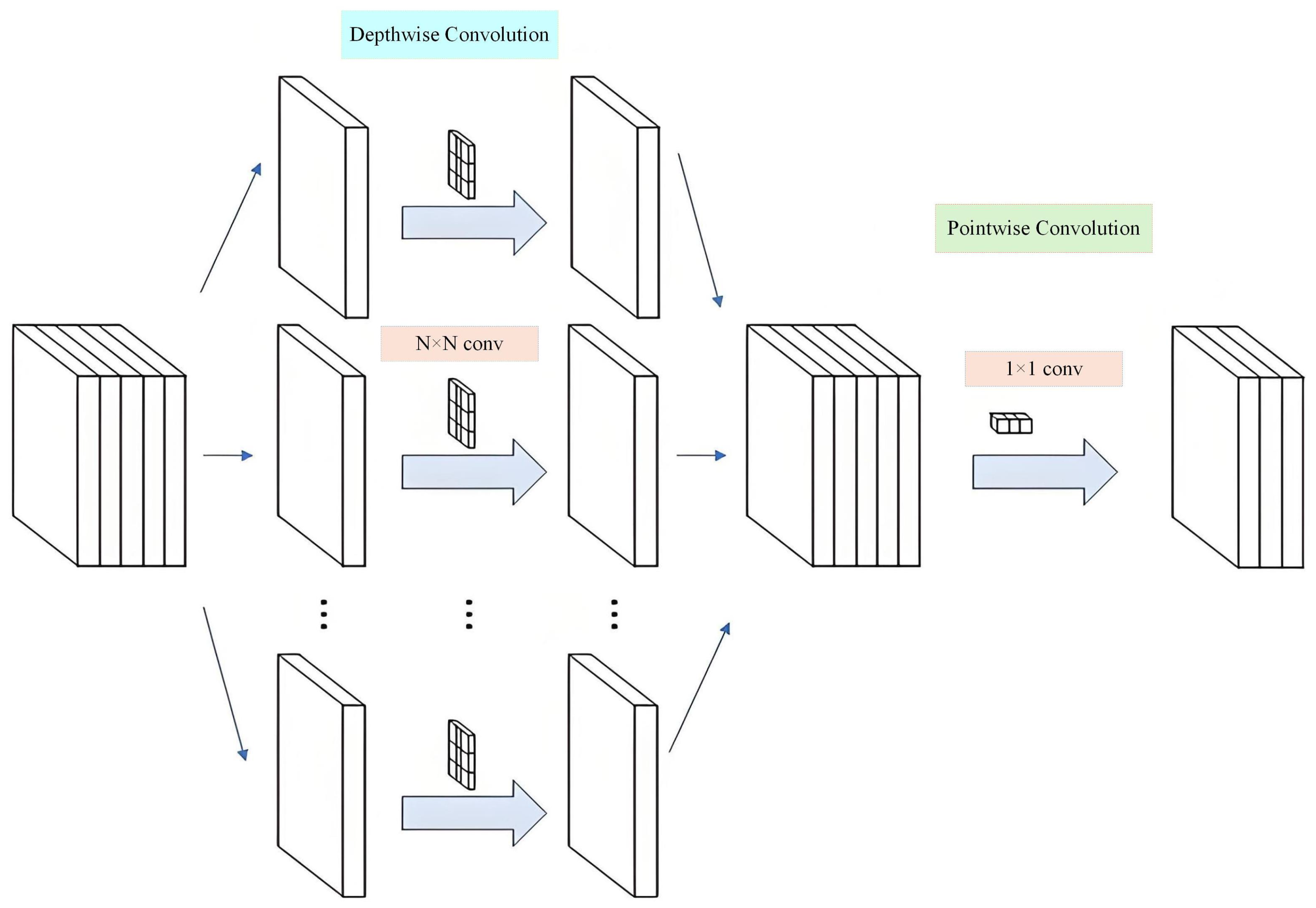
DSC is an efficient technique that splits convolution into two parts: Depthwise Convolution and Pointwise Convolution. Compared to traditional CNNs, DSC reduces both parameter and computational complexity, making it ideal for lightweight modeling and efficient feature extraction, as shown in Figure 3.

In short-term photovoltaic power generation prediction, the data is complex and heavily influenced by environmental factors like solar radiation, temperature, and humidity. Moreover, it exhibits significant spatial and temporal dependencies [27]. DSC is particularly well-suited for processing high-dimensional features. Through its two-stage convolution operation, DSC efficiently extracts essential information, preserving spatial relationships while enhancing the model’s expressive power, while reducing computational load.

The deep convolution operation extracts features by applying a convolution kernel to each input channel independently, and the output feature map has a smaller number of parameters. For the input feature map $X\in {\mathbb{R}}^{H\times W\times C_{\mathrm{in}}}$, the depth convolution operates independently on the spatial dimension H × W through the convolution kernel $K_c\in {\mathbb{R}}^{k\times k}$ of each channel to obtain the output $X_c^{\prime }$ of each channel:

$$X_c^{\prime }=X_c\ast K_c,c=1,2,\dots ,C_{\mathrm{in}}$$

(9)

where, ∗ represents the convolution operation, and the output $X_c^{\prime }$ is the feature map of the $X\in {\mathbb{R}}^{H\times W\times C_{\mathrm{in}}}$ channel.

2.5. Bidirectional Long Short-Term Memory

Although DSC improves the model’s operational efficiency by reducing computational complexity and the number of parameters. By utilizing both forward and backward information, BiLSTM improves the modeling of time-series features, enhancing the performance of short-term photovoltaic power generation predictions.The context vector and final output of BiLSTM can be obtained by Formulas (10)–(14).

$$\begin{array}{cc}\hfill h_t^{bi}& =[{\overrightarrow{h}}_t;{\overleftarrow{h}}_t]\hfill \end{array}$$

(10)

$$\begin{array}{cc}\hfill s_t& =\sum _{i=1}^T{\alpha }_{t,i}{h}_i^{bi}\hfill \end{array}$$

(11)

$$\begin{array}{cc}\hfill {\alpha }_{t,i}& ={\displaystyle \frac{exp\left(e_{t,i}\right)}{{\sum }_{j=1}^{T}exp\left(e_{t,j}\right)}}\hfill \end{array}$$

(12)

$$\begin{array}{cc}\hfill e_{t,i}& =v_a^{T}tanh(W_a{h}_t^{bi}+U_a{h}_i^{bi}+b_a)\hfill \end{array}$$

(13)

$$\begin{array}{cc}\hfill y_t& =\mathrm{softmax}(W_y{s}_t+b_y)\hfill \end{array}$$

(14)

where, $h_t^{bi}$ is Bi-directional hidden state at time t, formed by concatenating the forward and backward hidden states. The context vector $s_t$ at time t is a weighted sum of bi-directional hidden states. The attention weight ${\alpha }_{t,i}$ for the i hidden state is computed using softmax over attention scores $e_{t,i}$, which are calculated with a tanh activation. Finally, the output $y_t$ at time t is obtained by applying softmax to the context vector $s_t$.

The BiLSTM network has input, forget, and output gates that manage the flow of information. These gates help keep important temporal features and remove irrelevant data. The final hidden state is formed by merging the outputs from both the forward and backward LSTM layers. This structure enables the BiLSTM to capture dynamic patterns in short-term PV power generation time series, improving prediction stability and performance. The network structure is illustrated in Figure 4.

2.6. Convolutional Block Attention Module

While BiLSTM utilizes both forward and backward information to capture long-term dependencies in photovoltaic power time series data, it struggles to distinguish the importance of different time steps and feature channels. This limitation can lead to the model overlooking key information, impacting predictionperformance. To address this, the CBAM is introduced to optimize feature extraction and improve the model’s focus on critical information. The network structure with CBAM is shown in Figure 5.

The model incorporates Channel Attention (CA) and Spatial Attention (SA) to adjust feature map weights, focusing on key time steps and channels. Channel attention extracts global features using Global Average Pooling (GAP) and Global Max Pooling (GMP), and then calculates channel weights through a fully connected layer to emphasize important channels. Spatial attention captures critical spatial features through pooling and convolutional layers. In future work, we will conduct an interpretability analysis, using attention heatmaps and feature importance techniques to visualize and assess the relative importance of different channels and time steps. This will provide deeper insights into the model’s decision-making process.

2.7. The DSC-CBAM-BiLSTM Model

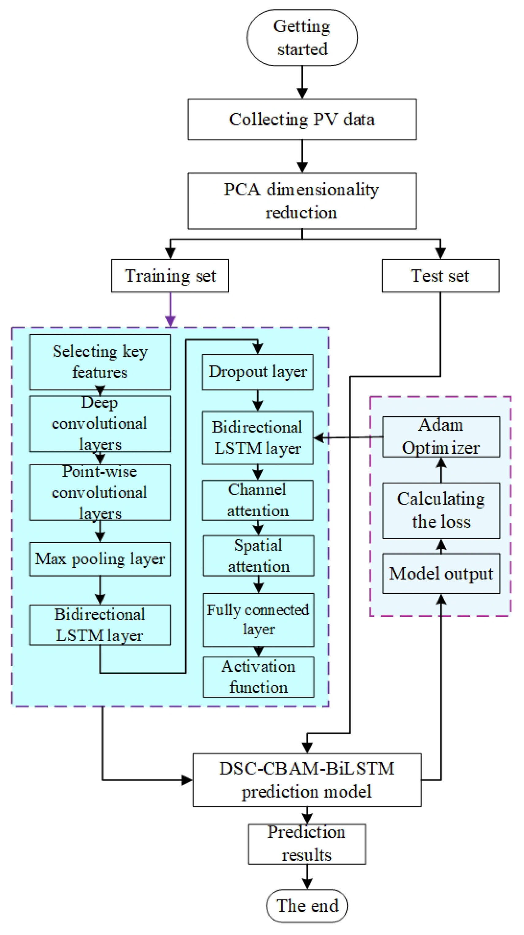
The construction process of the PPSO model involves five key stages: data preprocessing, feature selection, feature extraction, feature optimization, and time series modeling. PCA is used to reduce the dimensionality of the original PV data, eliminating redundancy while preserving key features. Then, the Particle Swarm PSO algorithm selects the optimal feature subset, enhancing prediction performance and lowering computational complexity. Then, a DSC is used to extract the local spatial features of the PV data, which are used as the initial state for the BiLSTM. Moreover, the channel spatial attention mechanism further enhances the key features. After feature extraction and optimization, the BiLSTM captures the dynamic trends in PV power changes more comprehensively, improving the stability of short-term predictions by combining forward and backward information. Finally, the output of the BiLSTM, optimized by CBAM weighting, is processed by a fully connected layer and passed through a Sigmoid activation function to obtain the predicted value of short-term PV generation.The flowchart is shown in Figure 6.

3. Experimental Environment

This section presents the key findings of the study, organized into three parts: experimental data selection and preprocessing, error analysis, and result analysis.

3.1. Data Selection and Preprocessing

The experimental data is collected from a photovoltaic power station in a specific area, covering the period from 17 June 2023, to 15 November 2023, with a 30-min sampling interval in megawatts (MW). The dataset includes features such as temperature, humidity, radiation intensity, wind speed, atmospheric pressure, power generation, season, and precipitation, among others. To ensure data quality, the original data is first preprocessed. Missing values are filled using linear interpolation, while outliers are detected using the box plot method (IQR), with values outside a reasonable range either corrected or removed. To eliminate the influence of feature dimensions, different features are normalized and preprocessed, ensuring that each feature is input to the model on the same scale. The dataset is then split into training and test sets, with a ratio of 8:2.

After preprocessing, PCA was used to convert correlated variables into a set of uncorrelated principal components ranked by their explained variance. As shown in

Table 1. Principal component contribution table.

Component	Eigenvalue	Variance Contribution (%)	Cumulative Contribution (%)
Temperature	45.28	45.32	45.32
Humidity	29.75	29.80	75.12
Radiation intensity	15.83	14.78	89.90
Atmospheric pressure	5.26	5.00	94.90
Wind speed	3.50	3.00	97.90
Precipitation	1.50	1.00	98.90
Season	0.80	0.20	99.10
Generation power	0.40	0.10	99.20

, the first four components account for over 89% of the total variance. This enables effective feature selection by retaining the most informative variables while reducing dimensionality and computational cost.

Table 1 shows the eigenvalues, variance contribution rates, and cumulative variance contributions for each principal component. Temperature, humidity, and radiation intensity contribute the most, with contribution rates of 45.32%, 29.80%, and 14.78%. These factors have a strong influence on the photovoltaic power prediction model. Atmospheric pressure, wind speed, precipitation, and season contribute less, with contribution rates of 5.00%, 3.00%, 1.00%, and 0.20%, respectively. Generation power has the smallest contribution at 0.10%.

In total, the first five components account for 97.90% of the total variance. These components are selected as the model’s initial input signals, which reduces redundancy and improves computational efficiency for the analysis and modeling.

3.2. Network Parameters

This study uses a structured model design and clear training settings to support the DSC-CBAM-BiLSTM model. The BiLSTM network has two layers, each with 128 hidden units per direction. The input size matches the selected feature dimension. A dropout rate of 0.3 helps prevent overfitting. The DSC layer uses 32 filters and a kernel size of 3. The CBAM module enhances key features. The output layer has 96 units for multi-step forecasting.

The model is trained using the Adam optimizer with a learning rate of 0.001 and batch size of 64. Training runs for 150 epochs with early stopping when the validation RMSE does not improve after 10 rounds. The validation set takes up 20% of the data. A fixed random seed ensures reproducibility.

3.3. Error Evaluation Index

To evaluate the prediction performance of different models, this paper uses the Mean Absolute Error (MAE), Root Mean Squared Error (RMSE), Accuracy, the coefficient of determination ($R^2$) as performance metrics and Confidence interval of RMSE ($C{I}_{RMSE}$). The formulas for these regression metrics are presented in Equations (15)–(19).

While these metrics are widely accepted for evaluating forecasting accuracy and model fit, we recognize the importance of additional statistical evaluations, such as confidence intervals, statistical significance tests, and robustness checks.

$$\mathrm{RMSE}=\sqrt{{\displaystyle \frac{1}{n}}\sum _{i=1}^n{(y_i-{\overline{y}}_i)}^2}$$

(15)

$$\mathrm{MAE}={\displaystyle \frac{1}{n}}\sum _{i=1}^n\left|y_i-{\overline{y}}_i\right|$$

(16)

$$R^2=1-{\displaystyle \frac{{\sum }_{i=1}^n{(y_i-{\overline{y}}_i)}^2}{{\sum }_{i=1}^n{(y_i-\overline{y})}^2}}$$

(17)

$$Accuracy={\displaystyle \frac{\mathrm{N}}{n}}\times 100\%$$

(18)

$$C{I}_{RMSE}=RMSE\pm Z_{\alpha /2}·SE\left(RMSE\right)$$

(19)

where, $y_i$ represents the true value, ${\widehat{y}}_i$ represents the predicted value, $\overline{y}$ is the mean value of the true values, and n represents the number of samples. N represents the number of correct predictions. $Z_{\alpha /2}$ is the critical value of the standard normal distribution, $SE\left(RMSE\right)$ is the standard error of RMSE, and $\alpha =0.05$ for a 95% confidence interval.

3.4. Prediction Results and Analysis

To evaluate the model’s performance across various training and validation sets, k-fold cross-validation is employed. The dataset is divided into five contiguous subsets based on time order, ensuring the continuity of the time series. The choice of a 5-month period is particularly meaningful, as it captures a range of diverse seasonal and weather conditions, which are essential for testing the model’s robustness in real-world PV forecasting scenarios.

By using this specific 5-month period, we ensure that the training and validation sets reflect typical operational timeframes, providing relevant insights into the model’s performance under realistic conditions. The division of these subsets is shown in

Table 2. Principal component contribution table.

Principal Name	Time Range
Sub 1	00:00 17 June 2023–24:00 15 July 2023
Sub 2	00:00 16 July 2023–24:00 15 August 2023
Sub 3	00:00 16 August 2023–24:00 15 September 2023
Sub 4	00:00 16 September 2023–24:00 15 October 2023
Sub 5	00:00 16 October 2023–24:00 15 November 2023

.

As shown in

Table 3. The K-fold cross-verification results.

Fold Number	Training Set	Validation Set	Average Error %	Accuracy %
1	sub 1,2,3,4	sub 5	5.23	85.4
2	sub 1,2,3,5	sub 4	4.76	86.3
3	sub 1,2,4,5	sub 3	5.14	84.9
4	sub 1,3,4,5	sub 2	4.95	86.1
5	sub 2,3,4,5	sub 1	5.08	85.7

, the model achieves an average error of 5.03% across all tests and an average performance of 85.7%, indicating stable behavior and strong predictive capability across diverse time periods. This reliability stems in part from our use of 5-fold cross-validation.

In 5-fold cross-validation, the dataset is divided into five equal parts. For each round, four parts are used for training and one for validation. This repeats five times so each part is a validation set once. The final results are the average of all five rounds. This method reduces bias from data splitting, ensuring the model performance is real and not overfitting. Though briefly mentioned before, 5-fold cross-validation is key to making our results reliable.

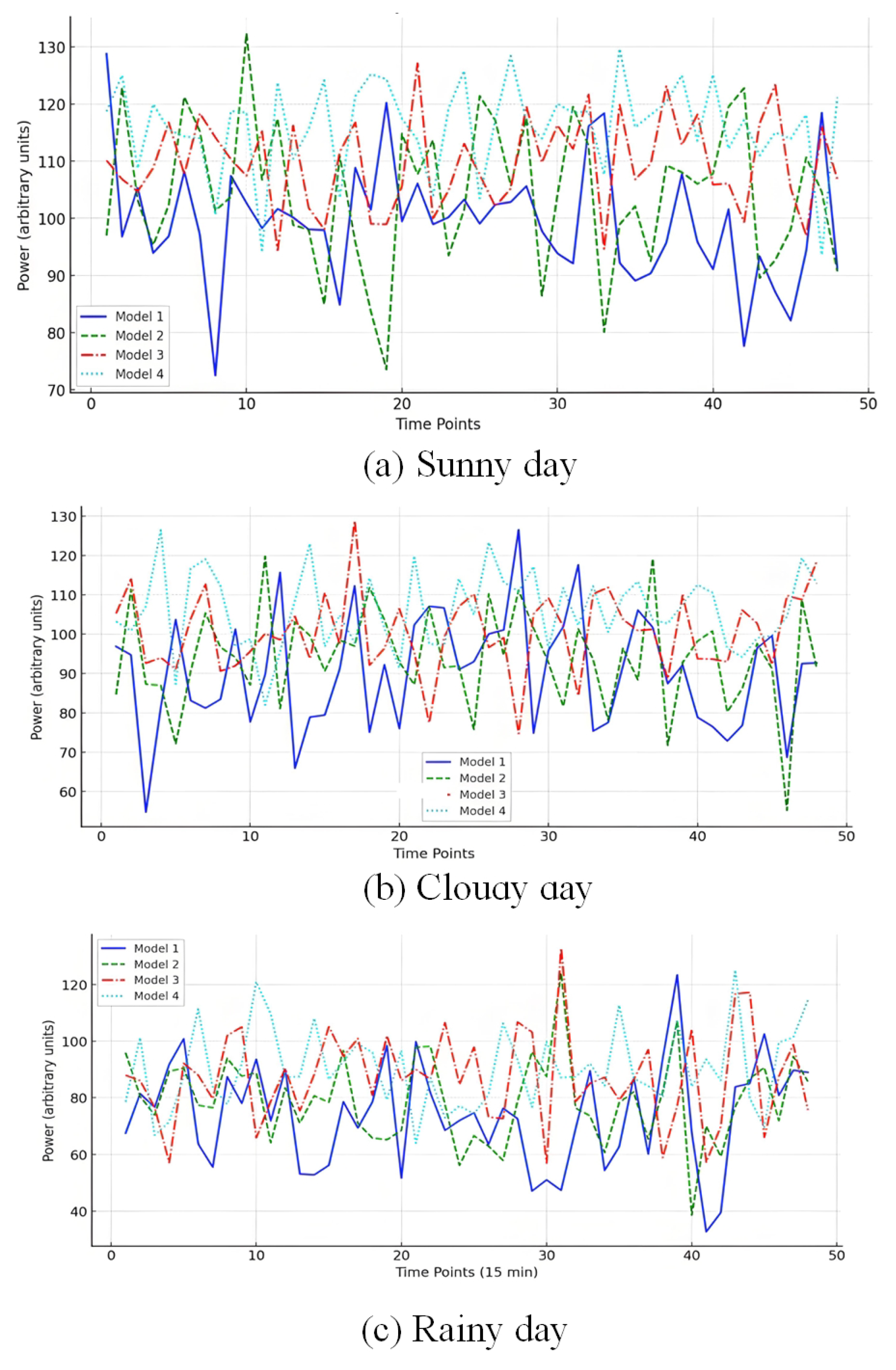
To evaluate the performance of the proposed DSC-CBAM-BiLSTM model, we compared it with DSC (Model 1), BiLSTM (Model 2), DSC-BiLSTM (Model 3), and DSC-BiLSTM-CBAM (Model 4) under various weather conditions. All models were tested using the same training and test sets, with consistent parameters, including the Adam optimizer, a PSO population size of 10, and a maximum of 100 iterations. Figure 7 illustrates the PV power predictions across different weather scenarios, demonstrating the reliability and effectiveness of the proposed model.

Figure 7 presents the predicted power output trends of different models under various weather conditions. On sunny days, the models show regular fluctuations, reflecting the predictable nature of photovoltaic (PV) generation. However, these curves alone are insufficient to claim that the predicted results “closely match” the actual values; quantitative error metrics are necessary for a more accurate assessment. Under cloudy conditions, power fluctuations become more complex due to factors like cloud movement and radiation changes. On rainy days, PV generation is more irregular and significantly impacted, consistent with the suppression of PV output in such weather. To better evaluate the prediction results across different conditions, we introduced a quantitative analysis, which is detailed in the

Table 4. Model Performance Across Different Weather Conditions with Confidence Intervals and Statistical Significance.

Weather	Model	RMSE	MAE	${\mathit{R}}^2$	CIRMSE
Sunny	model 1	8.265	6.125	0.894	[7.852, 8.678]
Sunny	model 2	6.674	5.836	0.918	[6.320, 7.028]
Sunny	model 3	2.438	1.653	0.935	[2.234, 2.642]
Sunny	model 4	2.126	1.476	0.954	[1.963, 2.289]
Cloudy	model 1	7.452	6.285	0.876	[7.112, 7.792]
Cloudy	model 2	7.004	5.105	0.894	[6.693, 7.315]
Cloudy	model 3	2.785	1.927	0.917	[2.596, 2.974]
Cloudy	model 4	2.467	1.706	0.936	[2.311, 2.623]
Rainy	model 1	8.053	7.727	0.854	[7.654, 8.452]
Rainy	model 2	7.574	6.301	0.887	[7.236, 7.912]
Rainy	model 3	3.206	2.053	0.905	[2.974, 3.438]
Rainy	model 4	2.853	1.832	0.927	[2.671, 3.035]

.

Table 4 shows the prediction results for each model under different weather conditions. It is clear that as the model is optimized, its prediction performance improves across all weather scenarios. On sunny days, Model 4 achieves the best performance, with an RMSE of 2.126, an MAE of 1.476, and an $R^2$ value of 0.954. These results indicate both high prediction accuracy and a strong fit to the data. Under cloudy conditions, Model 4 continues to outperform the other models. Although the RMSE (2.467) is slightly higher than on sunny days, it still delivers lower errors and a better fit, with an $R^2$ of 0.936. On rainy days, Model 4 remains the top performer, effectively predicting power generation data. These results demonstrate that, with continued optimization, the model’s performance improves across different weather conditions, with Model 4 being the most accurate under all scenarios.Additionally, the $C{I}_{RMSE}$ values are provided, representing the 95% confidence intervals of the RMSE. These intervals give a range within which the true RMSE is expected to fall with 95% confidence.

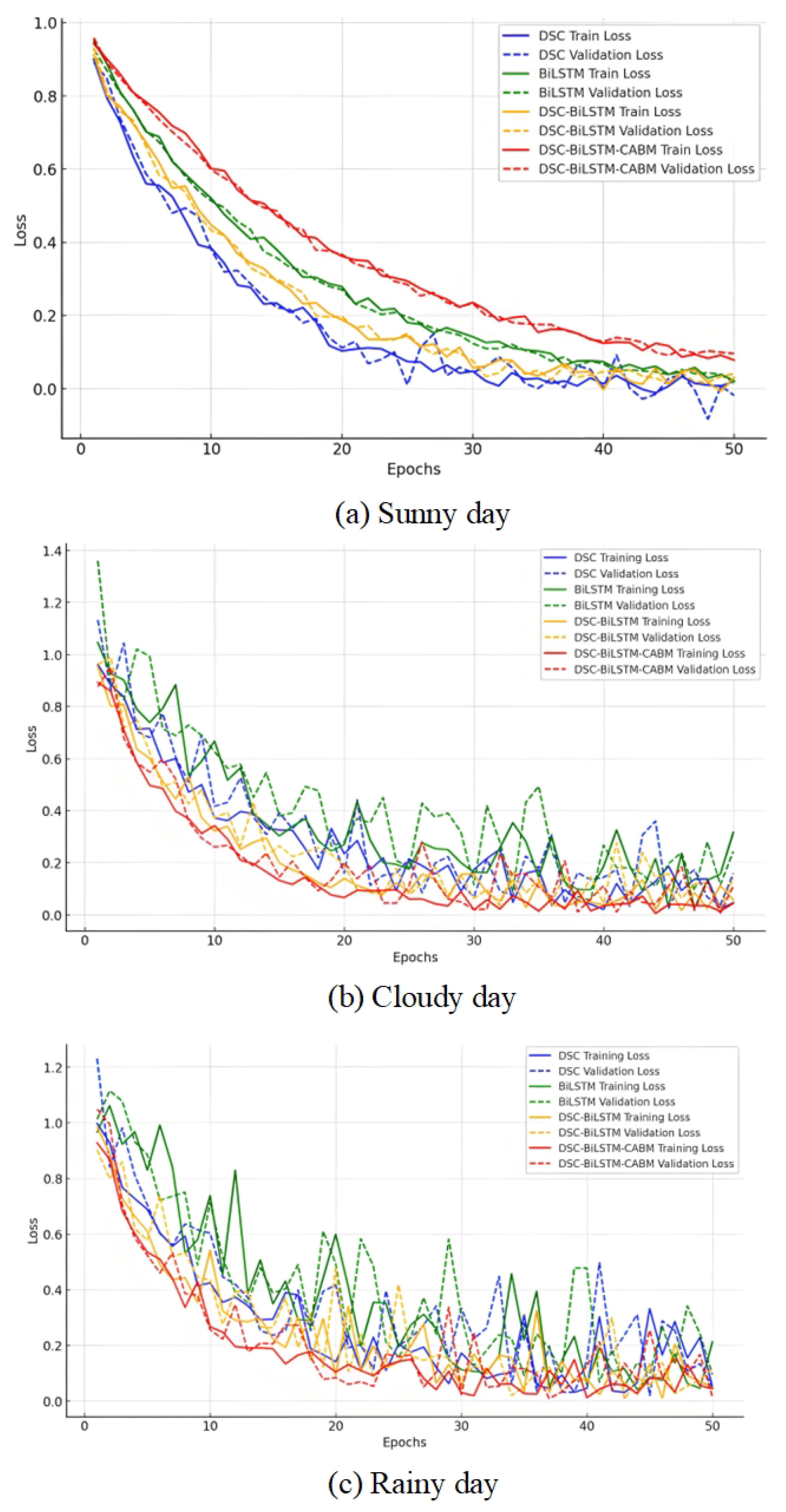
Figure 8 shows the loss curves for each model during training under different weather conditions. As the weather transitions from sunny to cloudy, and then to rainy, the loss curves of all models exhibit a gradual increase, with this effect being more pronounced under more complex weather conditions. This trend demonstrates the challenges in model generalization as weather conditions become more unpredictable. Specifically, the blue line representing the DSC model shows a noticeable rise in loss, particularly under cloudy and rainy conditions, suggesting limited generalization ability. Similarly, the green line for the BiLSTM model also experiences increased loss during more complex weather transitions, although its performance remains somewhat more stable than that of the DSC model.

In contrast, the yellow line for the DSC-BiLSTM model exhibits a better performance, especially under cloudy and rainy conditions, indicating the benefit of combining both the DSC and BiLSTM models. However, the red line, which represents the DSC-BiLSTM-CBAM model, consistently shows the best performance across all weather conditions, with much lower and more stable loss curves. This indicates that the CBAM module plays a crucial role in enhancing the model’s overall performance, particularly when facing more complex and variable weather conditions. Under sunny weather, all models converge relatively smoothly, but as the conditions shift to cloudy and rainy, the loss becomes more volatile, and the generalization ability of the models, except for the DSC-BiLSTM-CBAM model, is significantly compromised.

4. Conclusions

This study proposes DSC-BiLSTM-CBAM, a novel short-term photovoltaic power prediction model. By integrating PCA for dimensionality reduction, PSO for parameter optimization, DSC for efficient spatial feature extraction, CBAM for adaptive feature emphasis, and BiLSTM for capturing nonlinear temporal patterns, the model overcomes the limitations of traditional methods. Experiments show the model outperforms others in various weather, with RMSE down 74.3%, MAE 75.9%, and R-squared up 8.5%, proving its superior performance, stability, and adaptability to complex meteorological changes for practical value.

Future research will improve model generalization via advanced feature selection, including deep learning methods, and adopt statistical tools such as significance tests, and robustness checks to ensure result reliability. We also aim to incorporate real-time data for dynamic predictions and extend the model to longer-term forecasting and other renewables like wind and hydropower, enhancing scalability and practical use.

References

1. Rao, Z.; Yang, Z.; Li, J.; Li, L.; Wan, S. Prediction of Photovoltaic Power Generation Based on Parallel Bidirectional Long Short-Term Memory Networks. Energy Rep. 2024, 112, 3620–3629. [Google Scholar] [CrossRef]
2. Gao, X.; Zang, Y.; Ma, Q.; Liu, M.; Cui, Y.; Dang, D. A Physics-Constrained Deep Learning Framework Enhanced with Signal Decomposition for Accurate Short-Term Photovoltaic Power Generation Forecasting. Energy 2025, 326, 136220. [Google Scholar] [CrossRef]
3. Rathore, A.; Gupta, P.; Sharma, R.; Singh, R. Day Ahead Solar Forecast Using Long Short-Term Memory Network Augmented with Fast Fourier Transform-Assisted Decomposition Technique. Renew. Energy 2025, 247, 123021. [Google Scholar] [CrossRef]
4. Chen, F.; Ding, J.; Zhang, Q. A PV Power Forecasting Based on Mechanism Model-Driven and Stacking Model Fusion. J. Electr. Eng. Technol. 2024, 19, 4683–4697. [Google Scholar] [CrossRef]
5. Aman, R.; Dilshod, M.; Ulmas, Z.; Kumar, A.; Rizwan, M. A novel hybrid GWO-Bi-LSTM-based metaheuristic framework for short-term solar photovoltaic power forecasting. J. Renew. Sustain. Energy 2025, 17, 046101. [Google Scholar] [CrossRef]
6. Quan, R.; Qiu, Z.; Wan, H.; Yang, Z.; Li, X. Dung Beetle Optimization Algorithm-Based Hybrid Deep Learning Model for Ultra-Short-Term PV Power Prediction. iScience 2024, 27, 111126. [Google Scholar] [CrossRef] [PubMed]
7. Deng, H.; Alkhayyat, A. Sentiment analysis using long short term memory and amended dwarf mongoose optimization algorithm. Sci. Rep. 2025, 15, 17206. [Google Scholar] [CrossRef]
8. Dimitriadis, C.N.; Passalis, N.; Georgiadis, M.C. A Deep Learning Framework for Photovoltaic Power Forecasting in Multiple Interconnected Countries. Sustain. Energy Technol. Assess. 2025, 77, 104330. [Google Scholar] [CrossRef]
9. Pereira, S.; Canhoto, P.; Oozeki, T.; Salgado, R. Comprehensive Approach to Photovoltaic Power Forecasting Using Numerical Weather Prediction Data, Physics-Based Models, and Data-Driven Techniques. Renew. Energy 2025, 251, 123495. [Google Scholar] [CrossRef]
10. Xu, X.; Guan, L.; Wang, Z.; Yao, R.; Guan, X. A Double-Layer Forecasting Model for PV Power Forecasting Based on GRU-Informer-SVR and Blending Ensemble Learning Framework. Appl. Soft Comput. 2025, 172, 112768. [Google Scholar] [CrossRef]
11. Fan, S.; Geng, H.; Zhang, H. Multi-Step Power Forecasting Method for Distributed Photovoltaic (PV) Stations Based on Multimodal Model. Sol. Energy 2025, 298, 113572. [Google Scholar] [CrossRef]
12. Wang, R.; Ma, R.; Zeng, L.; Yan, Q.; Johnston, A.J. Improved Bidirectional Long Short-Term Memory Network-Based Short-Term Forecasting of Photovoltaic Power for Different Seasonal Types and Weather Factors. Comput. Electr. Eng. 2025, 123 Pt C, 110219. [Google Scholar] [CrossRef]
13. Souhe, F.G.Y.; Mbey, C.F.; Kakeu, V.J.F.; Meyo, A.E.; Boum, A.T. Optimized forecasting of photovoltaic power generation using hybrid deep learning model based on GRU and SVM. Electr. Eng. 2024, 106, 7879–7898. [Google Scholar] [CrossRef]
14. Min, H.; Noh, B. SolarNexus: A Deep Learning Framework for Adaptive Photovoltaic Power Generation Forecasting and Scalable Management. Appl. Energy 2025, 391, 125848. [Google Scholar] [CrossRef]
15. Li, J.; Rao, C.; Gao, M.; Xiao, X.; Goh, M. Efficient Calculation of Distributed Photovoltaic Power Generation Power Prediction via Deep Learning. Renew. Energy 2025, 246, 122901. [Google Scholar] [CrossRef]
16. Cubillo-Leyton, P.I.; Montoya, O.D.; Grisales-Noreña, L.F. Optimized Integration of Photovoltaic Systems and Distribution Static Compensators in Distribution Networks Using a Novel Discrete-Continuous Version of the Adaptive JAYA Algorithm. Results Eng. 2025, 26, 104726. [Google Scholar] [CrossRef]
17. Pattnaik, S.R.; Bisoi, R.; Dash, P.K. Solar Irradiance Forecasting Using Hybrid Long-Short-Term-Memory Based Recurrent Ensemble Deep Random Vector Functional Link Network. Comput. Electr. Eng. 2025, 123 Pt C, 110174. [Google Scholar] [CrossRef]
18. Fu, J.; Sun, Y.; Li, Y.; Wang, W.; Wei, W.; Ren, J.; Han, S.; Di, H. An Investigation of Photovoltaic Power Forecasting in Buildings Considering Shadow Effects: Modeling Approach and SHAP Analysis. Renew. Energy 2025, 245, 122821. [Google Scholar] [CrossRef]
19. Zayed, M.E.; Rehman, S.; Elgendy, I.A.; Al-Shaikhi, A.; Mohandes, M.A.; Irshad, K.; Abdelrazik, A.S.; Alam, M.A. Benchmarking Reinforcement Learning and Prototyping Development of Floating Solar Power System: Experimental Study and LSTM Modeling Combined with Brown-Bear Optimization Algorithm. Energy Convers. Manag. 2025, 332, 119696. [Google Scholar] [CrossRef]
20. Liu, J.; Zang, H.; Cheng, L.; Ding, T.; Wei, Z.; Sun, G. Robust Photovoltaic Power Forecasting Against Multi-modal Adversarial Attack via Deep Reinforcement Learning. IEEE Trans. Sustain. Energy 2025, 213, 16397. [Google Scholar] [CrossRef]
21. Şener, İ.F.; Tuğal, İ. Optimized CNN-LSTM with Hybrid Metaheuristic Approaches for Solar Radiation Forecasting. Case Stud. Therm. Eng. 2025, 72, 106356. [Google Scholar] [CrossRef]
22. Sardarabadi, A.; Heydarian Ardakani, A.; Matrone, S.; Ogliari, E.; Shirazi, E. Multi-temporal PV Power Prediction Using Long Short-Term Memory and Wavelet Packet Decomposition. Energy AI 2025, 21, 100540. [Google Scholar] [CrossRef]
23. Yang, K.; Cai, Y.; Cheng, J. A Deep Learning Model Based on Multi-Attention Mechanism and Gated Recurrent Unit Network for Photovoltaic Power Forecasting. Comput. Electr. Eng. 2025, 123, 110250. [Google Scholar] [CrossRef]
24. Alharthi, Y.; Chiroma, H.; Gabralla, L. Enhanced framework embedded with data transformation and multi-objective feature selection algorithm for forecasting wind power. Sci. Rep. 2025, 15, 16119. [Google Scholar] [CrossRef]
25. Yunqiao, L.; Yan, F. An innovative power prediction method for bifacial PV modules. Electr. Eng. 2023, 105, 2151–2159. [Google Scholar] [CrossRef]
26. Yang, D.Y.; Zhang, Z.; Gao, H.; Lv, Y. Variational Autoencoder-Based Learning Intrinsic Periodic-Trend Representations of Power Load Series for Short-Term Forecasting. Energy Rep. 2025, 13, 6584–6595. [Google Scholar] [CrossRef]
27. Li, J.; Ren, X.; Zhang, F.; Li, J.; Liu, Y. A Novel Deep Learning-Based Method for Theoretical Power Fitting of Photovoltaic Generation. Renew. Energy 2025, 250, 123271. [Google Scholar] [CrossRef]
Figure 1. The flowchart of the PSO algorithm.
Mathematics 13 02581 g001
Figure 2. Improved structure of the long short-term memory neural network model.
Mathematics 13 02581 g002
Figure 3. Depth-separable convolution structure diagram.
Mathematics 13 02581 g003
Figure 4. BiLSTM network structure.
Mathematics 13 02581 g004
Figure 5. CBAM network structure.
Mathematics 13 02581 g005
Figure 6. The flowchart of DSC-CBAM-BiLSTM.
Mathematics 13 02581 g006
Figure 7. Photovoltaic power prediction results for various weather conditions.
Mathematics 13 02581 g007
Figure 8. Photovoltaic power prediction results across different weather conditions.
Mathematics 13 02581 g008