Article

LLM-Guided Ensemble Learning for Contextual Bandits with Copula and Gaussian Process Models

1
Statistics Discipline, Division of Science and Mathematics, University of Minnesota-Morris, Morris, MN 56267, USA
2
EGADE Business School, Tecnológico de Monterrey, Ave. Rufino Tamayo, Monterrey 66269, Mexico
Mathematics 2025, 13(15), 2523; https://doi.org/10.3390/math13152523
Submission received: 7 July 2025 / Revised: 22 July 2025 / Accepted: 4 August 2025 / Published: 6 August 2025
(This article belongs to the Special Issue Privacy-Preserving Machine Learning in Large Language Models (LLMs))

Abstract

Contextual multi-armed bandits (CMABs) are vital for sequential decision-making in areas such as recommendation systems, clinical trials, and finance. We propose a simulation framework integrating Gaussian Process (GP)-based CMABs with vine copulas to model dependent contexts and GARCH processes to capture reward volatility. Rewards are generated via copula-transformed Beta distributions to reflect complex joint dependencies and skewness. We evaluate four policies—ensemble, Epsilon-greedy, Thompson, and Upper Confidence Bound (UCB)—over 10,000 replications, assessing cumulative regret, observed reward, and cumulative reward. While Thompson sampling and LLM-guided policies consistently minimize regret and maximize rewards under varied reward distributions, Epsilon-greedy shows instability, and UCB exhibits moderate performance. Enhancing the ensemble with copula features, GP models, and dynamic policy selection driven by a large language model (LLM) yields superior adaptability and performance. Our results highlight the effectiveness of combining structured probabilistic models with LLM-based guidance for robust, adaptive decision-making in skewed, high-variance environments.

1. Introduction

CMABs provide a principled framework for sequential decision-making under uncertainty, where an agent repeatedly selects actions (arms) based on observed context to maximize cumulative reward [1,2]. CMABs have been successfully applied in diverse fields including online advertising, recommendation systems, clinical trials, and financial trading [3].
The MAB framework balances exploration and exploitation to optimize decisions under uncertainty [4,5]. When side information or covariates are available at each decision step, contextual bandits exploit this additional information to improve learning and decision quality [2].
GP regression has emerged as a powerful tool for modeling unknown reward functions in CMABs [6,7,8]. GPs offer a nonparametric and probabilistic approach, capturing uncertainty naturally and enabling effective policies like Thompson Sampling (TS) and UCB. However, many practical scenarios involve complex, heteroskedastic, and dependent context variables that violate standard GP assumptions of independent and homoskedastic inputs.
To better reflect these complexities, we simulate covariates exhibiting volatility and nonlinear dependencies. Volatility is modeled using GARCH processes [9,10], capturing time-varying variance patterns common in finance and other domains. Dependence structures among features are represented with vine copulas [11,12], which flexibly model complex, high-dimensional dependencies beyond Gaussian assumptions. After applying the probability integral transform to normalize covariates, these enriched contexts create realistic and challenging bandit environments. Reward generation uses Beta distributions parameterized by the simulated volatility to encode heterogeneity and skewness [13]. Ref. [14] considered a novel generative-adversarial network algorithm, which is a deep learning algorithm, meticulously trained for the seismic inversion process. Recent breakthroughs in LLMs, such as GPT-4 [15], demonstrate remarkable ability in contextual understanding, summarization, and reasoning. Motivated by this, our approach integrates LLMs to assist both reward prediction and dynamic policy selection. The LLM reviews recent bandit performance and recommends strategies—including TS, UCB, Epsilon-Greedy, or a hybrid ensemble—to adaptively improve decision-making, especially in nonstationary or uncertain settings.
Building on prior work that combines copula-based context generation with GP reward modeling [16], our framework uniquely integrates LLM-driven guidance, yielding a flexible and interpretable model that leverages both structured probabilistic inference and deep language understanding. Simulation experiments with 10,000 independent runs demonstrate improved cumulative rewards and reduced regret compared to standard baselines, underscoring the benefits of this hybrid approach.
This paper addresses existing gaps by proposing a comprehensive simulation and modeling framework that functions as follows:
  • Employs vine copulas to capture rich, nonlinear dependencies among contextual variables;
  • Incorporates GARCH processes to simulate heteroskedastic, non-Gaussian reward noise;
  • Utilizes GP-based bandit policies enhanced with dynamic, LLM-guided policy selection;
  • Demonstrates through extensive experiments the superiority of this integrated approach in managing skewed, heavy-tailed, and volatile reward distributions.
Our contributions advance the state of the art by bridging structured probabilistic modeling with powerful LLM-based reasoning to improve adaptability and robustness in complex CMAB scenarios.
The rest of the paper is organized as follows. Section 2 introduces our model and reviews related literature on bandits, GPs, copulas, GARCH models, and LLMs. Section 3 details the simulation setup and empirical results. Section 4 concludes with final remarks and directions for future work.

2. Methods

2.1. Overview

We propose a hybrid simulation framework that integrates heteroskedastic contextual generation, copula-based dependence modeling, GP reward estimation, and LLM-guided policy selection. This framework enables evaluation and comparison of adaptive contextual bandit algorithms under realistic, complex environments.

2.2. Context Generation via GARCH and Copula Modeling

2.2.1. GARCH(1,1) Volatility Modeling

To capture time-varying volatility and heteroskedasticity in the context features x t = ( x t 1 , , x t , d ) , we simulate each dimension j = 1 , , d independently using a standard GARCH(1,1) process [9,13]:
σ t , j 2 = ω + α ϵ t 1 , j 2 + β σ t 1 , j 2 ,
where
  • σ t , j 2 is the conditional variance of dimension j at time t;
  • ω > 0 is the long-term variance constant;
  • α 0 measures sensitivity to recent squared innovations ϵ t 1 , j 2 ;
  • β 0 captures the persistence of past variance σ t 1 , j 2 ,
with the stationarity condition α + β < 1 ensuring that variance remains bounded over time [13].
The innovations ϵ t , j are assumed to be independent and identically distributed standard normal variables:
ϵ t , j N ( 0 , 1 ) .
The observed contextual feature for dimension j at time t is generated as:
x t , j = σ t , j · z t , j , z t , j N ( 0 , 1 ) ,
where z t , j is an independent noise term. This standard GARCH(1,1) setup captures typical volatility clustering found in financial and many real-world time series [9,17].

2.2.2. Copula-Based Dependence Modeling

To model nonlinear and flexible dependencies among the d contextual features, we apply a vine copula approach [11,12]. After transforming the marginals to uniform variables via the probability integral transform (PIT), the vine copula captures complex joint dependence structures beyond Gaussian correlation assumptions.
This integration of GARCH-driven heteroskedastic marginals with vine copula dependence provides a realistic and challenging environment for contextual bandit algorithms. While the GARCH model and vine copula construction follow established methodologies [11,13], our contribution lies in coupling these components within a unified simulation framework to generate realistic, time-varying, and dependent contexts for evaluating adaptive bandit policies.

2.2.3. Copula-Based Dependence Structure

To model cross-sectional dependence among the d contextual features at each time step t, we employ a copula-based approach [11,18]. This separates marginal behavior from the dependence structure, offering greater flexibility in simulating realistic multivariate contexts.
First, each contextual variable x t , j is transformed into a uniform score using the empirical cumulative distribution function (ECDF), which serves as a rank-based approximation:
u t , j = rank ( x t , j ) T + 1 ,
where
  • u t , j ( 0 , 1 ) is the pseudo-observation of the j-th variable at time t;
  • rank ( x t , j ) is the rank of x t , j among { x 1 , j , , x T , j } ;
  • T is the total number of observations.
This yields the vector u t = ( u t , 1 , , u t , d ) ( 0 , 1 ) d , which represents the transformed context in the copula space.
To model dependencies among these uniform variables, we fit a regular vine copula (R-vine) to the observed { u t } t = 1 T . An R-vine decomposes the joint copula density into a cascade of bivariate (pair) copulas organized in a sequence of linked trees, allowing rich and flexible modeling of high-dimensional dependencies [11,12].
Once the R-vine copula C is estimated, we apply the inverse copula transform as follows:
v t = C 1 ( u t ) ,
where C 1 denotes the inverse transform (sampling from the copula distribution). The resulting v t R d encodes dependencies among contextual features and is used as input to the contextual bandit policy.
This copula-based preprocessing allows the simulation of dependent and potentially non-Gaussian context vectors with realistic structure and tail dependence. Such features are often found in domains like finance, environment, and health care, where multivariate covariates are rarely independent.

2.3. Reward Simulation

For a contextual bandit problem with K arms, we simulate bounded stochastic rewards r t ( k ) [ 0 , 1 ] at each time step t using the inverse cumulative distribution function (CDF) of the Beta distribution. The reward for each arm is generated based on its associated copula-transformed contextual variable v t , k ( 0 , 1 ) , as follows:
r t ( k ) = F Beta 1 ( v t , k ; α , β ) ,
where
  • r t ( k ) denotes the reward for arm k { 1 , , K } at time t;
  • v t , k is the PIT-transformed contextual input for arm k, obtained through a copula model to capture dependence across arms;
  • F Beta 1 ( · ; α , β ) is the inverse CDF (quantile function) of the Beta distribution;
  • α > 0 and β > 0 are shape parameters controlling the distribution’s skewness and variance.
The Beta distribution is flexible and supported on the interval [ 0 , 1 ] , making it well-suited for modeling bounded rewards. By adjusting the following shape parameters:
  • Higher values of α relative to β result in right-skewed distributions (more probability mass near 1);
  • Higher values of β relative to α lead to left-skewed distributions (more mass near 0);
  • Equal values of α and β yield symmetric distributions (e.g., the uniform distribution when α = β = 1 ).
This reward mechanism allows context-dependent simulation of non-Gaussian, heteroskedastic, and skewed reward profiles, reflecting many real-world environments such as treatment effects, conversion probabilities, or user responses.

2.4. GP Reward Estimation

To model the unknown reward function f k ( · ) for each arm k { 1 , , K } , we use independent GP regressions. Each GP is trained on the PIT-transformed contexts v t [ 0 , 1 ] d and the corresponding rewards r t ( k ) , using the training dataset { ( v t , r t ( k ) ) } t = 1 T train . This approach follows the probabilistic regression framework outlined in [8]:
f k ( v ) GP ( m k ( v ) , k k ( v , v ) ) ,
where
  • f k ( v ) is the latent reward function for arm k evaluated at input v [ 0 , 1 ] d ;
  • GP ( · , · ) denotes a GP prior;
  • m k ( v ) = E [ f k ( v ) ] is the mean function, often assumed to be zero;
  • k k ( v , v ) = Cov ( f k ( v ) , f k ( v ) ) is the covariance (kernel) function, typically chosen as the squared exponential (RBF) kernel, as follows:
    k k ( v , v ) = σ f 2 exp 1 2 2 v v 2 ,
    with hyperparameters (length-scale) and σ f 2 (signal variance).
After training, the GP provides closed-form posterior predictive distributions for unseen inputs v * , yielding the following:
  • Predictive mean μ k ( v * ) = E [ f k ( v * ) D k ] ;
  • Predictive variance σ k 2 ( v * ) = Var [ f k ( v * ) D k ] ,
where D k = { ( v t , r t ( k ) ) } t = 1 T train is the training data for arm k.
These predictive statistics are used in downstream bandit policies—e.g., UCB and TS—allowing principled exploration under uncertainty.

2.5. Bandit Policies and LLM Integration

2.5.1. Classical Policies

We compare three classical MAB policies that trade off between exploration (trying new arms) and exploitation (selecting the current best arm), all using GP posterior reward models.
  • TS: For each round t, the algorithm draws a sample from the GP posterior predictive distribution for each arm k given the current context v t , and selects the arm with the highest sampled reward:
    a t = arg max k r ˜ t ( k ) , r ˜ t ( k ) N ( μ k ( v t ) , σ k 2 ( v t ) ) ,
    where μ k ( v t ) and σ k 2 ( v t ) are the GP posterior predictive mean and variance for arm k. This method balances exploration and exploitation through posterior sampling [7].
  • UCB: At each time t, the algorithm selects the arm that maximizes an upper confidence bound:
    a t = arg max k μ k ( v t ) + κ σ k ( v t ) ,
    where
    μ k ( v t ) is the GP posterior predictive mean;
    σ k ( v t ) is the posterior predictive standard deviation;
    κ > 0 is a tunable parameter that controls the degree of exploration.
    Larger values of κ favor more exploration. This approach encourages arms with either high expected reward or high uncertainty [1].
  • Epsilon-Greedy: This strategy selects the empirically best arm (highest predicted mean reward) with probability 1 ε , and a random arm with probability ε as follows:
    a t = arg max k μ k ( v t ) , with probability 1 ε , random arm k , with probability ε ,
    where ε [ 0 , 1 ] is a hyperparameter controlling exploration [5].

2.5.2. Ensemble Policy with LLM Guidance

We propose an ensemble bandit policy that integrates structured statistical modeling via GPs with unstructured, semantic reasoning from a LLM. For a given context vector v t R d , arm index k { 1 , , K } , and historical regret summary h t , the ensemble reward prediction is defined as follows:
r ^ t , k = ( 1 w ) · μ k ( v t ) + w · LLM _ pred ( v t , k , h t ) ,
where
  • μ k ( v t ) is the posterior predictive mean reward for arm k under the GP model, given the PIT-transformed context v t ;
  • LLM _ pred ( v t , k , h t ) is the reward estimate from an LLM (e.g., GPT-4 [15]) conditioned on contextual information and a summary of recent regret or reward history h t ;
  • w [ 0 , 1 ] is a tunable weighting hyperparameter that balances the contribution of model-based statistical prediction and LLM-based semantic inference.
The ensemble decision rule selects the arm maximizing r ^ t , k across all k as follows:
a t = arg max k r ^ t , k .
The parameter w can be:
  • Fixed: chosen via offline validation (e.g., cross-validation or grid search) to minimize cumulative regret;
  • Adaptive: dynamically updated during online learning, for instance by tracking the relative predictive accuracy or uncertainty of the GP and LLM components.
This flexible ensemble allows the policy to leverage the statistical rigor of GPs (which are effective when sufficient data is available) while integrating high-level semantic reasoning from the LLM, which may capture patterns not explicitly encoded in the structured data. Empirically, moderate values of w (e.g., w [ 0.3 , 0.5 ] ) often achieve a strong balance between interpretability and adaptivity.

2.6. Adaptive Policy Selection via LLM

To enhance flexibility and responsiveness in sequential decision-making, we introduce an adaptive policy selection mechanism that leverages a LLM to choose a policy at each time step t > t 0 . The candidate policy set includes the following:
P = T S , U C B , Epsilon-greedy , ensemble .
At each decision point t, the LLM is prompted with a natural language summary of recent performance metrics—such as cumulative reward, rolling regret, arm selection diversity, and historical policy usage. The model then recommends a policy π t P to be applied at time t. This adaptive strategy enables the agent to dynamically shift between exploration and exploitation, or between structured and semantic reasoning, depending on evolving environmental conditions.
To mitigate premature reliance on the LLM and ensure a stable foundation of training data, we define a **delay threshold** t 0 N , such that:
  • For t t 0 , actions are selected using classical model-based policies (e.g., TS or UCB), relying exclusively on GP reward estimates μ k ( v t ) .
  • For t > t 0 , the LLM is queried to determine either the next policy π t or to provide reward guidance through the ensemble formulation (see Equation (7)).
In our empirical setup, we fix t 0 = 100 , which provides a sufficient warm-up phase for GPs to form reliable posterior distributions. This threshold can also be made **adaptive** in future work, e.g., by monitoring, as follows:
  • convergence of posterior uncertainty ( σ k ( v t ) );
  • stabilization of cumulative regret slopes;
  • entropy of policy selection history.
Overall, this framework empowers the bandit agent to transition from purely statistical decision-making to a hybrid regime incorporating external semantic reasoning from foundation models like GPT-4 [15].

2.7. LLM Prompt Engineering

We integrate a LLM, specifically GPT-4 [15], into our contextual bandit simulation to support both reward prediction and adaptive policy selection. The LLM is queried using structured prompts that encapsulate the current context, reward history, and policy performance summaries. This allows the model to inject high-level reasoning and learned patterns into the decision-making process.

2.7.1. Reward Prediction Prompt

To estimate the expected reward for a given arm k under context v t = ( v t , 1 , v t , 2 , , v t , d ) R d , the LLM is queried with the following prompt structure:
Given context vector: v t , 1 , v t , 2 , , v t , d , and arm index: k, along with recent reward history: [summary of last m rewards], predict the reward in the range [0, 1].
This prompt instructs the LLM to return a scalar estimate r ^ t , k LLM [ 0 , 1 ] , interpreted as the predicted reward for arm k at time t. The recent reward history provides grounding information to contextualize predictions. To ensure stability, the decoding temperature is set to a low value (e.g., 0.2–0.3), promoting deterministic outputs.

2.7.2. Policy Selection Prompt

For adaptive policy selection, the LLM receives a summary of recent performance statistics:
“Given recent bandit performance metrics: [tabular summary of last n rounds including rewards, regrets, and selected policies], choose one policy from: TS, UCB, Epsilon-greedy, ensemble. Respond with only the policy name.”
This prompt yields a discrete choice π t LLM P , where P = { TS , UCB , Epsilon-greedy , ensemble } . The LLM leverages observed patterns in regret and reward trends to recommend the most contextually appropriate policy. By restricting the output format, we reduce parsing complexity and enhance reliability.

2.7.3. Caching and Robustness

To reduce API latency and ensure deterministic behavior, we implement query-level caching. Identical prompts yield reused outputs. If the LLM returns invalid or missing results, the system defaults to a safe fallback strategy (e.g., Thompson Sampling), preserving robustness throughout the simulation pipeline.

2.8. Evaluation Metrics

We employ a suite of quantitative metrics to evaluate the performance of contextual bandit policies, focusing on learning efficiency, stability, and adaptivity.

2.8.1. Cumulative Regret

The primary metric is the cumulative regret  R t , defined as the total difference between the reward of the optimal arm and that of the selected arm up to time t as follows:
R t = s = 1 t max k { 1 , , K } r s ( k ) r s ( a s ) ,
where r s ( k ) [ 0 , 1 ] is the reward that would have been received if arm k had been selected at time s, a s { 1 , , K } is the arm actually selected at time s.
Lower values of R t indicate more effective exploration and faster convergence to optimal behavior.

2.8.2. Cumulative and Average Reward

We also track the cumulative reward and average reward:
CumulativeReward t = s = 1 t r s ( a s ) , AverageReward t = 1 t s = 1 t r s ( a s ) .
These metrics reflect how well the algorithm exploits learned knowledge to obtain high rewards over time.

2.8.3. Confidence Intervals and Replications

To assess variability and statistical reliability, all simulations are repeated independently N times. At each time step t, we compute the sample mean m ¯ t and standard deviation s t for a metric of interest (e.g., regret or reward). The associated 95% confidence interval is:
CI t = m ¯ t ± 1.96 · s t N .
These intervals are used to visualize uncertainty and support statistical comparisons across policies.

2.8.4. Policy Switching Dynamics

For adaptive systems (e.g., LLM-guided policies), we track the frequency with which each policy p P is selected at time t. Let π t ( p ) [ 0 , 1 ] denote the proportion of times policy p was selected at time t across replications. These usage patterns are visualized with stacked area plots to characterize dynamic policy adaptation.

2.8.5. Per-Arm Performance

We summarize per-arm statistics such as the following:
-
Mean reward received when each arm k was selected;
-
Selection frequency per arm under each policy p.
This breakdown reveals how well different policies identify and exploit specific arms, highlighting arm-specific strengths and weaknesses.
The integration of LLM prompt engineering with classical bandit policies, along with robust evaluation metrics, enables comprehensive benchmarking of adaptive bandit algorithms under complex contextual conditions, including heteroskedasticity and temporal dependencies.

3. Simulation Setup

We conduct a comprehensive simulation study to evaluate the performance of several contextual bandit policies under structured, time-varying reward heterogeneity. Our framework integrates functional volatility dynamics, copula-based dependency modeling, and GP regression for reward prediction. We also incorporate LLM-guided decision-making policies in a hybrid setup.

3.1. Context Generation via Functional Volatility and Copula Transformation

To simulate heteroskedastic, non-Gaussian, and dependent contextual variables, we construct a matrix of contextual features
X t R T × d
driven by volatility dynamics and copula-based dependence modeling. Here:
  • X t is the matrix of contextual features with T time points and d feature dimensions;
  • Each row x t R d represents the context vector at time t.
  • Heteroskedastic Context Generation
Each contextual dimension follows an sGARCH(1,1) process, as follows:
σ t , j 2 = ω + α 1 ε t 1 , j 2 + β 1 σ t 1 , j 2 ,
where
  • σ t , j 2 is the conditional variance of dimension j at time t;
  • ω = 0.1 is the constant base volatility;
  • α 1 = 0.15 controls sensitivity to past shocks ε t 1 , j 2 ;
  • β 1 = 0.7 governs persistence of volatility;
  • ε t , j N ( 0 , 1 ) are independent standard normal innovations;
  • Stationarity is ensured by α 1 + β 1 < 1 .
Each dimension j = 1 , , d evolves independently according to this process.
  • Copula-Based Dependency Modeling
To capture dependencies among the d contextual features,
  • We transform the GARCH-generated contexts into pseudo-observations U t , j [ 0 , 1 ] using empirical cumulative distribution function (CDF) ranks as follows:
    U t , j = 1 T + 1 s = 1 T 1 ( x s , j x t , j ) ,
    ensuring uniform marginals suitable for copula modeling;
  • A high-dimensional Vine Copula is fitted to the data U t = ( U t , 1 , , U t , d ) using the RVineStructureSelect algorithm;
  • This copula captures flexible nonlinear and tail dependencies between features;
  • The probability integral transform (PIT) from the fitted copula yields the final transformed contextual inputs U ˜ t , which serve as bandit model inputs.
  • Time-Varying Reward Volatility
To model nonstationary reward noise, we simulate GARCH(1,1) volatility for each arm’s reward noise:
σ t , k 2 = ω + α ϵ t 1 , k 2 + β σ t 1 , k 2 ,
where
  • σ t , k 2 is the conditional reward variance for arm k at time t;
  • ω = 0.1 , α = 0.1 , and β = 0.8 are fixed parameters;
  • ϵ t , k represents reward noise innovations;
  • These parameters model volatility persistence ( α + β < 1 ) and responsiveness to recent shocks;
  • This setup reflects financial-style volatility clustering to stress-test policy robustness under realistic, time-varying uncertainty.
We have the following attentions:
  • Distinguish volatility variables: σ t , j 2 for context dimension j, σ t , k 2 for arm k’s reward volatility;
  • GARCH introduces temporal dependence, while Vine Copula models cross-sectional dependence among contexts;
  • Each arm’s reward noise is modeled separately to allow arm-specific volatility dynamics.

3.2. Reward Generation

To simulate nonlinear, context-dependent reward functions, we define the arm-level reward distributions via a monotonic mapping from the copula-transformed contextual variable U ˜ t to the inverse CDF of a Beta distribution as follows:
Y t , a Beta 1 ( U ˜ t , a ; α , β ) , a = 1 , , A ,
where
  • Y t , a is the reward at time t for arm a;
  • A is the total number of arms;
  • U ˜ t , a [ 0 , 1 ] is the probability integral transform (PIT) value corresponding to arm a at time t, obtained from copula-based transformations of context;
  • Beta 1 ( · ; α , β ) is the quantile function (inverse cumulative distribution function) of the Beta distribution parameterized by positive shape parameters α , β .
The shape parameters α and β control the skewness and concentration of the reward distribution as follows:
  • α = 2 , β = 5 produces a left-skewed distribution (mass near 0), modeling sparse or conservative rewards;
  • α = 5 , β = 2 produces a right-skewed distribution (mass near 1), modeling optimistic rewards with heavier tails.
This construction ensures that rewards are nonlinear and heterogeneous functions of the context and arm.

3.3. Reward Modeling via Gaussian Processes

Each arm-specific reward function f a ( · ) is modeled with a GP regression as follows:
f a ( x ) GP ( 0 , k ( x , x ) ) ,
where
  • f a ( x ) is the unknown reward function for arm a evaluated at context x R d ;
  • The mean function is assumed zero for simplicity;
  • The covariance kernel k ( x , x ) is the squared exponential (RBF) kernel, given by
    k ( x , x ) = σ f 2 exp x x 2 2 l 2 + g δ x x ,
    where
    σ f 2 is the signal variance;
    l is the length-scale controlling smoothness;
    g = 10 6 is a small noise term (nugget) added for numerical stability;
    δ x x is the Kronecker delta function (1 if x = x , else 0).
Posterior means μ t , a and variances σ t , a 2 from the GP are used to guide uncertainty-aware exploration policies.

3.4. Bandit Policies Evaluated

We compare several contextual bandit policies. For each time t, given posterior mean μ t , a and variance σ t , a 2 for arm a, the policies are:
  • TS: Sample a reward
    Y ˜ t , a N ( μ t , a , σ t , a 2 ) ,
    then select the arm with the highest sampled reward:
    a t = arg max a Y ˜ t , a .
  • UCB: Select the arm maximizing the UCB score:
    a t = arg max a μ t , a + 2 log ( t ) · σ t , a 2 ,
    balancing exploitation and exploration.
  • Epsilon-Greedy: With probability ε = 0.1 , select a random arm; otherwise, select the arm with the highest posterior mean:
    a t = arg max a μ t , a .
  • LLM-Guided Policies:
    LLM-Reward: Uses predicted reward estimates from an LLM (mocked in simulation) to select the arm with highest predicted reward;
    LLM-Policy: Dynamically selects among TS, UCB, Epsilon-greedy, or LLM-Reward policies by querying an LLM based on recent performance summaries.

3.5. Simulation Protocol

  • Total time steps: T = 100 ;
  • Context dimension: d = 10 ;
  • Number of arms: A = 3 .
The first 70% of data is used to train arm-specific GP models, and the last 30% is reserved for bandit simulation. At each time t, given context x t , the selected arm a t receives reward Y t , a t .

3.6. Evaluation Metrics and Replications

We evaluate each policy over R = 10,000 Monte Carlo replications, computing the following:
  • Mean Reward:
    1 R r = 1 R Y t , a t ( r ) ,
    where Y t , a t ( r ) is the reward at time t for replication r.
  • Cumulative Regret:
    Regret t ( r ) = s = 1 t max a Y s , a ( r ) Y s , a s ( r ) ,
    representing the cumulative loss compared to always playing the best arm.
  • Confidence Intervals (95%):
    x ¯ t ± 1.96 s t R ,
    where x ¯ t is the empirical mean and s t is the sample standard deviation over replications.

3.7. Empirical Results

Table 1 compares the performance of four contextual bandit policies:
  • LLM-Reward: A policy guided by LLM reward prediction;
  • Epsilon-Greedy: Selects a random arm with probability ε = 0.1 , otherwise exploits the best-known arm;
  • UCB: Selects arms by maximizing upper confidence bounds to balance exploration and exploitation;
  • TS: Samples from posterior reward distributions for probabilistic action selection.
The table reports the following metrics under two different Beta-distributed reward regimes, Y t , a Beta 1 ( α , β ) :
  • Mean R: Average reward obtained by the policy; higher values indicate better performance;
  • SD R: Standard deviation of the reward across replications; lower values indicate more stable results;
  • Mean Reg: Mean cumulative regret, defined as the total difference between the optimal arm’s reward and the chosen arm’s reward; lower values indicate more efficient learning;
  • SD Reg: Standard deviation of cumulative regret, reflecting variability in performance across replications.
The reward regimes are:
  • α = 2 , β = 5 : Left-skewed Beta distribution modeling sparse or conservative rewards.
  • α = 5 , β = 2 : Right-skewed Beta distribution modeling optimistic rewards with heavier tails.
The results demonstrate that the LLM-Reward policy consistently attains the highest mean reward and lowest regret, indicating superior decision-making. The Epsilon-Greedy policy shows competitive mean reward but suffers from higher variability. Meanwhile, UCB and TS underperform under both regimes, suggesting limited adaptability to complex or asymmetric reward landscapes.
Figure 1 (Cumulative Regret Over Time) plots the cumulative regret
R t = s = 1 t max a r s , a r s , a s ,
where r s , a is the reward of arm a at time s, and a s is the selected arm. Lower R t indicates more efficient learning. The figure shows that TS and the LLM-guided policy maintain the lowest regret growth, reflecting better exploration-exploitation trade-offs, whereas UCB and ϵ -greedy accumulate more regret over time.
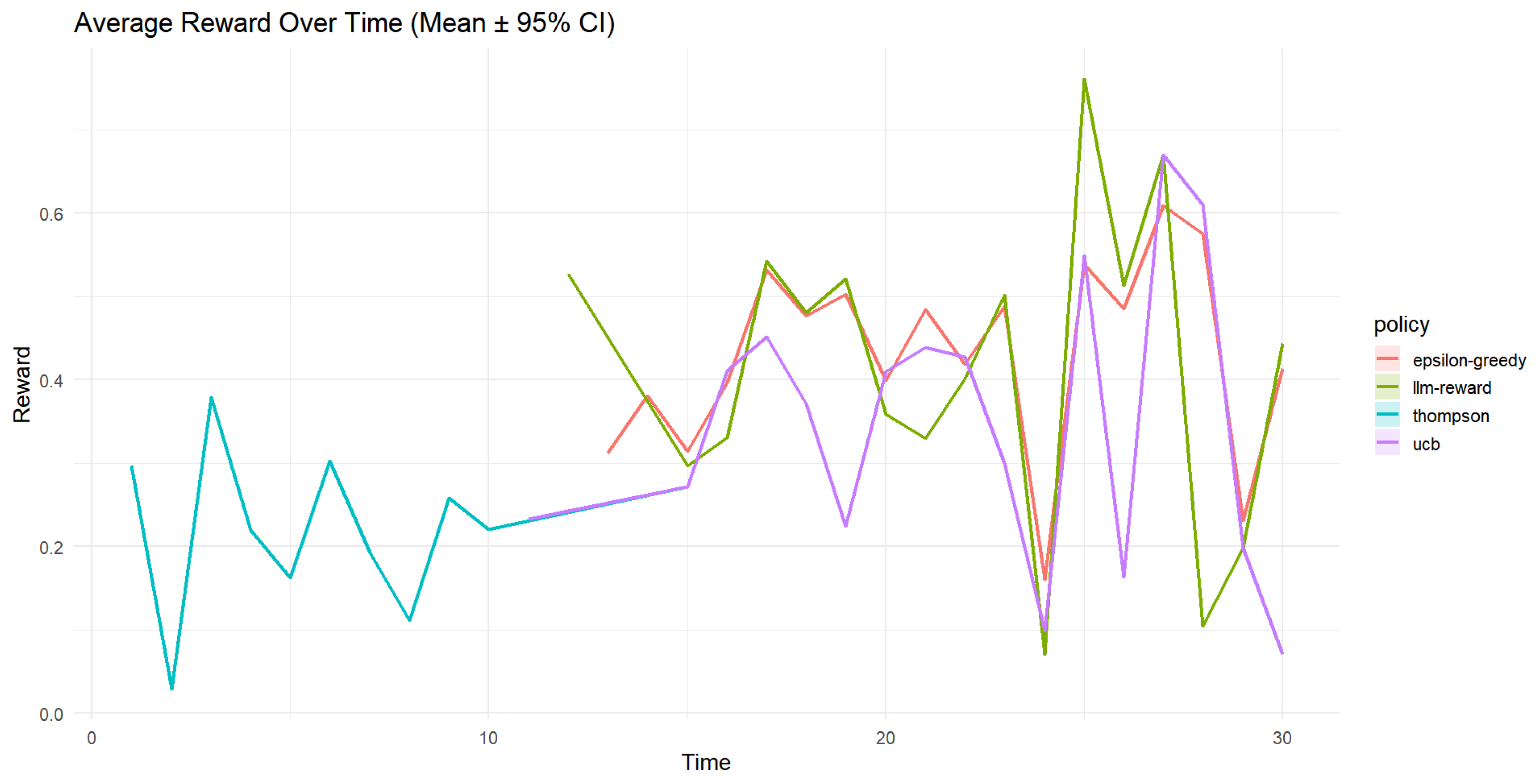
Figure 2 (Average Reward Over Time) displays the average reward trajectory, highlighting that TS and LLM-guided policies generally achieve higher and more stable rewards. The ϵ -greedy policy exhibits high variance, reflecting less reliable learning.
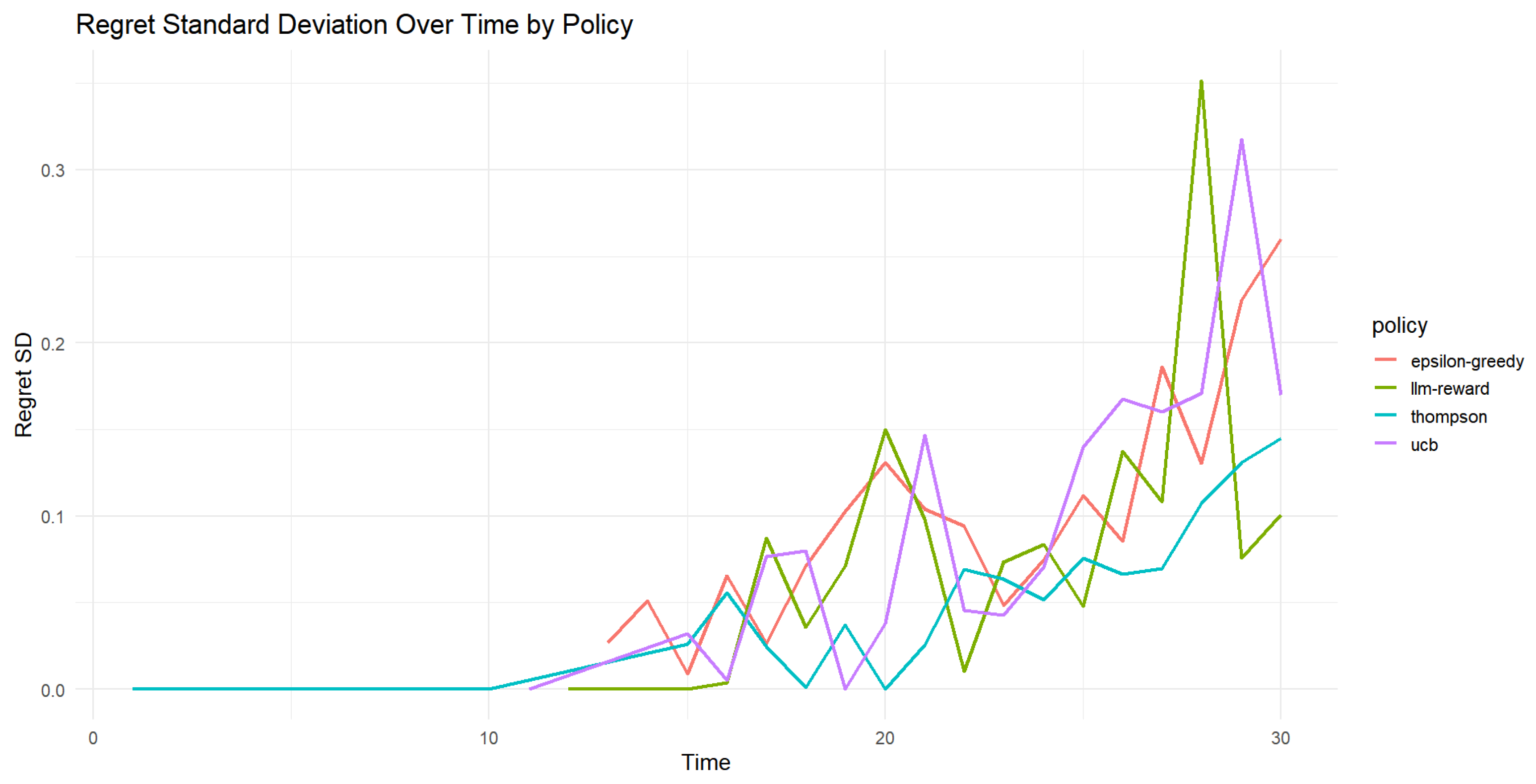
Figure 3 (Regret Standard Deviation Over Time) assesses the consistency of policies by plotting the standard deviation of cumulative regret across simulation replications. Lower values indicate more stable and reliable learning behavior. Thompson and LLM policies show more stability early in learning, though all policies experience increased variability after around time step 20, potentially due to the heavy-tailed nature of the Beta reward distributions causing occasional outlier outcomes.
The notation Y t , a Beta 1 ( α , β ) indicates that rewards for arm a at time t are generated via the inverse cumulative distribution function (quantile function) of the Beta distribution with shape parameters α and β . This modeling induces skewness and heteroskedasticity in rewards, challenging standard bandit algorithms.
The empirical results illustrate that LLM-guided policies effectively leverage contextual and historical information to achieve robust performance across different reward distribution shapes and volatility, while classical policies like UCB and TS can struggle under these complex settings.
The use of 95% confidence intervals in the figures supports rigorous statistical interpretation, while regret metrics emphasize the fundamental exploration-exploitation balance inherent in sequential decision-making.
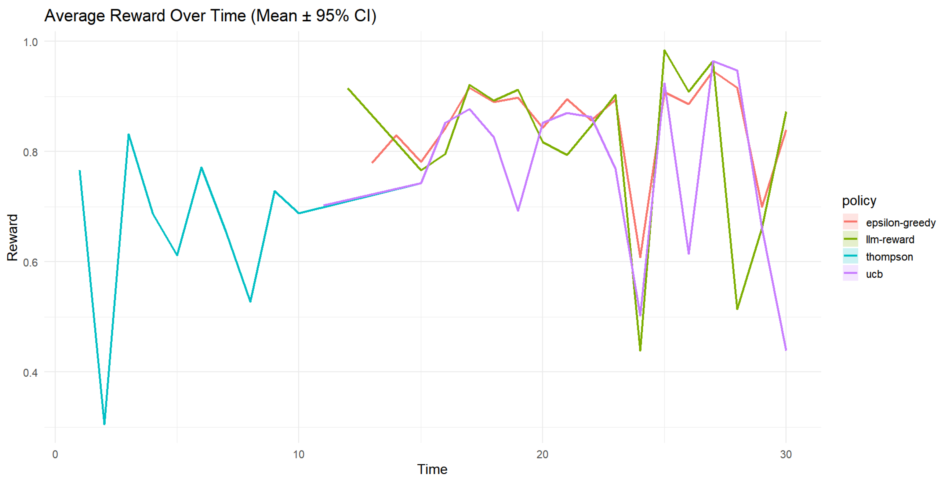
Figure 4, Figure 5 and Figure 6 illustrate the performance of contextual bandit policies under a left-skewed inverse Beta reward distribution Y t , a Beta 1 ( 5 , 2 ) . This setup introduces significant variability and a greater likelihood of extreme reward values concentrated near the upper bound.
The notation Y t , a Beta 1 ( α , β ) indicates that the reward for arm a at time t is generated by the inverse cumulative distribution function (quantile function) of a Beta distribution with shape parameters α and β . Here, α = 5 and β = 2 specify a left-skewed distribution. Cumulative regret R t = s = 1 t max a Y s , a Y s , a s measures the accumulated loss due to suboptimal arm selections up to time t. The plotted confidence intervals represent 95% uncertainty bounds around the mean metrics.
This plot compares the accumulation of regret over time across policies. The TS and LLM-guided policies achieve the lowest cumulative regret, indicating efficient exploration-exploitation trade-offs and rapid adaptation to arms with higher rewards despite the skewed distribution. In contrast, the ϵ -greedy policy exhibits a significantly steeper regret curve, reflecting slower learning caused by excessive random exploration.
The average reward trajectories demonstrate that TS and LLM policies quickly converge to high-reward arms, effectively capitalizing on the tail behavior of the skewed reward distribution. The UCB policy performs moderately well but is consistently outperformed by the LLM and Thompson approaches. The ϵ -greedy policy shows lagging and erratic performance, likely due to over-exploration.
This figure depicts the standard deviation of regret across repeated simulations, reflecting policy stability. Early in the simulation, TS and LLM-guided policies maintain lower variability, indicating more stable and reliable learning. However, all policies exhibit increasing variability in later stages, attributable to the heavy-tailed reward distribution producing occasional extreme outcomes. The Epsilon-greedy strategy remains the most unstable throughout.
The results collectively highlight that distribution-aware exploration strategies, such as TS and LLM-informed policies, handle skewed, high-variance reward environments more effectively than heuristic approaches like UCB or Epsilon-greedy. Incorporating LLM-based guidance alongside flexible probabilistic context modeling offers tangible advantages in complex sequential decision-making scenarios.

4. Conclusions

This study evaluates the performance of four contextual bandit policies—Ensemble, Epsilon-greedy, Thompson Sampling, and UCB—through extensive simulation over 10,000 replications, focusing on cumulative regret, reward stability, and adaptive effectiveness under heavy-tailed and skewed reward distributions. In scenarios where rewards follow complex, asymmetric distributions, the Thompson Sampling and LLM-guided policies consistently demonstrate superior performance, maintaining lower cumulative regret and higher observed rewards compared to baselines. The Epsilon-greedy policy, in contrast, exhibits unstable behavior and higher regret variability over time.
In both symmetric and skewed reward settings, the ensemble policy—enhanced with copula-transformed contextual features and Gaussian Process-based modeling—achieves the most robust performance, consistently yielding the lowest regret and highest cumulative rewards. These findings underscore the importance of flexible modeling techniques and the integration of language model guidance for real-time contextual decision-making in dynamic environments.
Looking forward, we plan to explore lightweight LLM surrogates, caching mechanisms, and asynchronous decision-making pipelines to address latency concerns associated with real-world deployment. Further directions include meta-bandit frameworks for strategy adaptation and extending our approach to high-dimensional, spatio-temporal applications. Balancing the intelligence of LLMs with real-time operational constraints will be central to advancing practical, deployable contextual bandit systems.

Funding

This research received no external funding.

Institutional Review Board Statement

Not related in this research.

Data Availability Statement

No new data were created or analyzed in this study.

Acknowledgments

We thank the three respected referees, Associated Editor, and Editor for their constructive and helpful suggestions, which led to substantial improvement in the revised version. For the sake of transparency and reproducibility, the R code for this study can be found in the following GitHub repository: R code GitHub site (https://github.com/kjonomi/Rcode/blob/main/LLMbandits, accessed on 4 August 2025).

Conflicts of Interest

The authors declare no conflicts of interest.

References

  1. Auer, P.; Cesa-Bianchi, N.; Fischer, P. Finite-time analysis of the multiarmed bandit problem. Mach. Learn. 2002, 47, 235–256. [Google Scholar] [CrossRef]
  2. Langford, J.; Zhang, T. The Epoch-Greedy Algorithm for Multi-armed Bandits with Side Information. Adv. Neural Inf. Process. Syst. 2007, 20. [Google Scholar]
  3. Li, L.; Chu, W.; Langford, J.; Schapire, R.E. A contextual-bandit approach to personalized news article recommendation. In Proceedings of the 19th International Conference on World Wide Web, Raleigh, NC, USA, 26–30 April 2010; Association for Computing Machinery: New York, NY, USA, 2010. [Google Scholar] [CrossRef]
  4. Lai, T.L.; Robbins, H. Asymptotically efficient adaptive allocation rules. Adv. Appl. Math. 1985, 6, 4–22. [Google Scholar] [CrossRef]
  5. Sutton, R.S.; Barto, A.G. Reinforcement Learning: An Introduction, 2nd ed.; MIT Press: Cambridge, MA, USA, 2018. [Google Scholar]
  6. Srinivas, N.; Krause, A.; Kakade, S.M.; Seeger, M. Gaussian Process Optimization in the Bandit Setting: No Regret and Experimental Design. In Proceedings of the International Conference on Machine Learning (ICML), Haifa, Israel, 21–24 June 2010. [Google Scholar]
  7. Agrawal, S.; Goyal, N. Thompson Sampling for Contextual Bandits with Linear Payoffs. In Proceedings of the International Conference on Machine Learning (ICML), Atlanta, GA, USA, 16–21 June 2013. [Google Scholar]
  8. Rasmussen, C.E.; Williams, C.K.I. Gaussian Processes for Machine Learning; MIT Press: Cambridge, MA, USA, 2006. [Google Scholar]
  9. Engle, R.F. Autoregressive Conditional Heteroscedasticity with Estimates of the Variance of United Kingdom Inflation. Econometrica 1982, 50, 987–1007. [Google Scholar] [CrossRef]
  10. Zakoian, J.-M. Threshold Heteroskedastic Models. J. Econ. Dyn. Control 1994, 18, 931–955. [Google Scholar] [CrossRef]
  11. Aas, K.; Czado, C.; Frigessi, A.; Bakken, H. Pair-copula constructions of multiple dependence. Insur. Math. Econ. 2009, 44, 182–198. [Google Scholar] [CrossRef]
  12. Czado, C. Analyzing Dependent Data with Vine Copulas: A Practical Guide with R; Springer: Berlin, Germany, 2019. [Google Scholar]
  13. Bollerslev, T. Generalized autoregressive conditional heteroskedasticity. J. Econom. 1986, 31, 307–327. [Google Scholar] [CrossRef]
  14. Olya, B.A.M.; Mohebian, R.; Moradzadeh, A. A new approach for seismic inversion with GAN algorithm. J. Seism. Explor. 2024, 33, 1–36. [Google Scholar]
  15. OpenAI. GPT-4 Technical Report. 2023. Available online: https://arxiv.org/abs/2303.08774 (accessed on 10 May 2025).
  16. Kim, J.-M. Gaussian Process with Vine Copula-Based Context Modeling for Contextual Multi-Armed Bandits. Mathematics 2025, 13, 2058. [Google Scholar] [CrossRef]
  17. Francq, C.; Zakoian, J.-M. GARCH Models: Structure, Statistical Inference and Financial Applications, 2nd ed.; Wiley: Hoboken, NJ, USA, 2019. [Google Scholar]
  18. Nelsen, R.B. An Introduction to Copulas, 2nd ed.; Springer: Berlin, Germany, 2006. [Google Scholar]
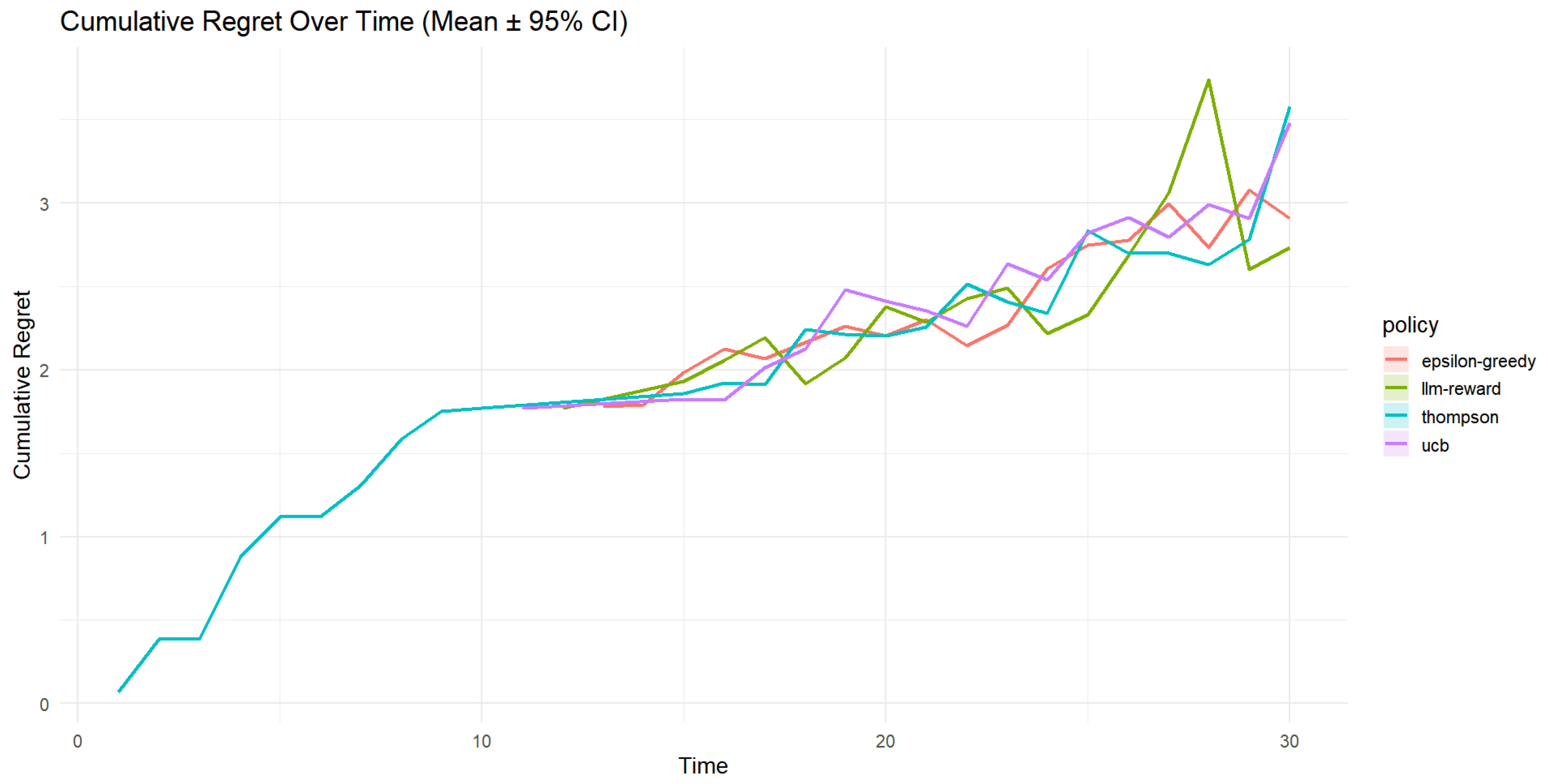
Figure 1. Cumulative regret over time (mean ± 95% CI) for the contextual bandit simulation where Y t , a Beta 1 ( 2 , 5 ) . Lower cumulative regret indicates better learning efficiency. TS and the LLM-guided policy exhibit lower regret growth compared to UCB and Epsilon-greedy, suggesting more efficient action selection over time.
Mathematics 13 02523 g001
Figure 2. Average reward over time (mean ± 95% CI) for Y t , a Beta 1 ( 2 , 5 ) . Higher average reward reflects better policy performance. Both TS and the LLM-guided policy consistently achieve higher average rewards, despite fluctuations due to the heavy-tailed reward structure. The ϵ -greedy policy shows substantial variability, indicating less reliable learning.
Mathematics 13 02523 g002
Figure 3. Regret standard deviation over time by policy under Y t , a Beta 1 ( 2 , 5 ) . This figure measures the consistency of each policy across repeated simulations. Lower standard deviation indicates more stable learning behavior. TS and the LLM-guided policy maintain lower regret variability in early stages, but all policies exhibit increased volatility after time step 20.
Mathematics 13 02523 g003
Figure 4. Cumulative regret over time (mean ± 95% CI) for the contextual bandit simulation with Y t , a Beta 1 ( 5 , 2 ) . The TS and LLM-guided policies again achieve the lowest cumulative regret. The ϵ -greedy policy performs worse, with a significantly steeper regret curve.
Mathematics 13 02523 g004
Figure 5. Average reward over time (mean ± 95% CI) for Y t , a Beta 1 ( 5 , 2 ) . The Thompson and LLM-based policies converge more quickly to high-reward arms. The ϵ -greedy policy lags behind and exhibits erratic performance, likely due to over-exploration.
Mathematics 13 02523 g005
Figure 6. Regret standard deviation over time by policy for Y t , a Beta 1 ( 5 , 2 ) . Thompson and LLM-guided policies display reduced variance in the early phase, indicating robust learning. However, all policies show increasing variability in later rounds, possibly due to the skewness and extreme values inherent in the reward distribution.
Mathematics 13 02523 g006
Table 1. Comparison of policy performance under different reward distributions.
PolicyMean RSD RMean RegSD RegMean RSD RMean RegSD Reg
Y t , a Beta 1 ( 2 , 5 ) Y t , a Beta 1 ( 5 , 2 )
LLM-Reward0.44400.00002.73000.11900.87300.00002.54000.1010
Epsilon-Greedy0.41400.09922.91000.27000.84000.11102.55000.2600
UCB0.07070.00003.48000.18300.43900.00003.10000.1700
Thompson0.07070.00003.58000.09110.43900.00003.26000.1450
Disclaimer/Publisher’s Note: The statements, opinions and data contained in all publications are solely those of the individual author(s) and contributor(s) and not of MDPI and/or the editor(s). MDPI and/or the editor(s) disclaim responsibility for any injury to people or property resulting from any ideas, methods, instructions or products referred to in the content.