Abstract
This paper is concerned with the problem of dynamic output feedback exponential stability control of T-S fuzzy networked control systems (NCSs) with varying communication delays. First, with consideration of varying communication delays, a new model of the networked systems is established by using the T-S fuzzy method, and a state observer is designed to estimate the unknown control disturbance. Then, a delay-dependent exponential stability criterion of closed-loop systems is derived by means of iterative technique and multiple augmented Lyapnov functionals and the linear matrix inequality (LMI) method. Furthermore, an observer-based controller is explicitly constructed to realize exponential stability control for this class of NCSs. An iterative algorithm is developed to compute the controller’s matrix by means of the Cone Complementarity Linearization Method (CCLM). Lastly, the validity and feasibility of the proposed exponential stability criterion are confirmed via a numerical simulation example.
MSC:
93D15; 93D23
1. Introduction
Networked control systems (NCSs) are network-based feedback control systems that utilize network technology to connect dispersed devices, sensors, and actuators, enabling information exchange as well as greatly improving the automation and intelligence level of the systems. Since its proposal at the end of the 20th century, NCSs have attracted widespread attention from both academia and industry [1,2,3]. Compared with traditional control systems, NCSs have advantages such as flexible structure, easy scalability, and resource sharing, providing new ideas and methods for the design, implementation, and maintenance of the control systems. However, the research on NCSs also faces some challenges, such as the introduction of networks, which make it difficult to avoid latency and packet loss issues. These problems may lead to a decrease in controller performance and even instability.
In recent years, with the rapid development of control, network, and communication technologies, NCSs have gradually become a hot research topic [4,5,6]. The research content covers multiple aspects such as modeling, time delay, stability analysis, disturbance handling, controller design, and performance evaluation. In terms of modeling, researchers are committed to establishing more accurate NCS models to better describe the dynamic behavior of the systems. These models help us to understand the operating mechanism of the systems and provide a foundation for subsequent control.
Time delay and stability are key issues in NCSs. Researchers have conducted extensive research on time delay compensation, stability analysis, and other aspects to improve the robustness and stability of the systems. Disturbance handling is also one of the important directions in the research of NCSs. In practical applications, the systems are often affected by various external disturbances, such as noise, interference, etc. In order to improve the anti-interference ability of the systems, researchers have conducted in-depth research on disturbance suppression, filtering algorithms, and other aspects. In addition, network predictor design, traffic optimization, controller design, and scheduling are also hot topics in the research of NCSs. In summary, the research status of NCSs shows a trend of diversification and deepening, covering multiple key issues and research directions. With the continuous advancement of technology and the expansion of application fields, research on NCSs will continue to deepen, providing more efficient and intelligent control solutions for fields such as industrial automation and intelligent transportation [7,8]. Kundu et al. studied the allocation of communication resources in networked control systems. A method for finding periodic scheduling strategies has been proposed, under which the global asymptotic stability of each system in NCSs is maintained. A stable scheduling strategy is built by using loops that satisfy appropriate contractility conditions on the underlying weighted directed graph of NCSs [9]. An improved algorithm has been proposed to accelerate the convergence speed of the network systems. By using smaller initial values and faster decay rates, a more accurate upper limit of the system states can be obtained. The effectiveness of the improvement was demonstrated through simulation [10]. The finite-time stabilization problem of a class of discrete-time networked control systems with network-induced delay, as well as packet loss in feedback and forward channels, was studied. A new finite-time state feedback and output feedback stable controller is proposed using predictive control methods, and compensation is made for time delay and packet loss. A sufficient condition for finite-time stabilization is given for a given discrete-time networked control system [11]. Chen et al. studies the delay-dependent state feedback control problem of a class of networked control systems with nonlinear disturbances and two delay components. Based on the dynamic delay interval method and Wirdinger integral inequality, some improved delay-dependent stability analyses have been obtained. Subsequently, the results were extended to NCSs with time delay, and the corresponding stability analysis results and state feedback controllers were obtained [12].
Fuzzy systems are intelligent control systems based on fuzzy mathematics theory, which uses language rules and fuzzy logic reasoning to make decisions. Fuzzy systems have been widely applied in various industries and practical applications [13,14,15,16,17]. In the industrial field, fuzzy control is applied in various aspects such as industrial furnaces, petrochemical processes, robot systems, etc. The advantages of fuzzy control systems are that they do not require the establishment of an accurate mathematical model of the controlled object, have simple designs, are easy to implement, and have strong robustness. However, fuzzy systems also have some drawbacks, such as simple fuzzy processing of information, which may lead to a decrease in control accuracy and a deterioration in dynamic quality of the systems. The design of fuzzy control still lacks systematicity, making it difficult to effectively control complex systems. Li et al. studied the defense control problem of T-S fuzzy systems with multiple transmission channels for sampled data against asynchronous denial-of-service (DoS) attacks. A new exchange security control method has been proposed to tolerate asynchronous DoS attacks that act independently on each channel. In addition, by applying the segmented Lyapunov function method, the sufficient conditions dependent on the membership function were derived to ensure the exponential stability of the systems [18]. The robust fuzzy control problem of the nonlinear systems with actuator saturation limitation was studied. By using T-S fuzzy description, a fuzzy observer is established based on the sampled output affected by the network-induced delay. The saturation fuzzy control law is derived from the estimated states of the observer [19]. Zheng et al. studied the dynamic output feedback and H∞ stability analysis of a class of uncertain networked control systems with multiple time delays and external disturbances. A delay-dependent Lyapunov functional with double-product sub-items was designed, and the stability conditions in the form of LMI were obtained to ensure asymptotic stability of the closed-loop systems under the specified H∞ performance [20].
T-S fuzzy logic systems is the abbreviation of Takagi–Sugeno fuzzy logic systems, which quantifies the consequent of each fuzzy rule in pure fuzzy logic systems [21,22,23,24]. The T-S fuzzy model is an effective tool for describing nonlinear systems, which represents the dynamic characteristics of the entire system by dividing the system into a set of local models and applying a set of linear feedback control laws in each local model. This method is particularly suitable for NCSs and can effectively solve the stability problem of nonlinear systems [25,26,27,28,29]. Pan et al. investigated the design problem of a security controller based on resilient event-triggering for a nonlinear NCSs described by interval type-2 fuzzy model under non-periodic denial-of-service attacks. A resilient event-triggering strategy based on uncertain event-triggered variables is proposed for nonlinear NCSs. This strategy can transmit necessary data packets to the controller in unexpected situations [30]. Aslam1 et al. investigated the output tracking control problem of a class of T-S fuzzy nonlinear network control systems. A strategy based on event-triggered scheme is proposed to reduce bandwidth utilization in NCSs by utilizing inherent constraints, including communication latency and data transmission limitations. On this basis, a synchronous behavior-based operation model is proposed to make the design of linear controllers easier to implement [31].
However, the above research has mainly focused on the asymptotic stability and control design of fuzzy network systems, while research on exponential stability and dynamic output feedback control is relatively rare. This article is based on previous research and focuses on a class of T-S fuzzy NCSs with time-varying delays. By constructing a new Lyapunov functional and using linear matrix inequality tools to design an exponential stable state observer for the systems, the sufficient conditions for the simultaneous exponential stability of the closed-loop systems and error systems are obtained. The design strategy of the exponential stable controller is given by using the observation data.
2. Preliminaries
Consider the following fuzzy NCSs with varying communication delays given in Figure 1 with the following state delay plant:
Rule :
If is and is , and is ,
Then ,
where is the premise variable, is the state, is the number of fuzzy rules, are the fuzzy sets, is the control input, is the controlled output, , , and are a set of known real matrices. is the initial condition of the state. is the varying state delay.

Figure 1.
A typical networked control system.
In Figure 1, and are the sensor–controller delay and controller–actuator delay, respectively. Then the communication delay is given by .
Assumption 1.
Only the output of the systems is available.
Assumption 2.
and are time-varying under the following bounded condition.
Using single-point fuzzification, a product inference engine, and the central fuzzy elimination method, the global fuzzy model of the systems (1) can be described as
where
whereis the membership degree ofcorresponding to, andsatisfies
And we define
In this paper, the following fuzzy observer of the systems (2) is designed
where is the state of the observer, and is a set of constant matrices to be determined.
The observer error is defined as
With (2)–(4), the error systems can be obtained as
where .
And then, a fuzzy controller based on the above observer is designed as
Using Equations (2), (4) and (6), the resultant closed-loop systems can be written as
Before establishing our main results, the following basic definition and Lemma are given.
Definition 1
([7]). For the systems (2), if there exist constants and such that
Lemma 1
([8]). The linear matrix inequality
Remark 1.
By taking the delay from sensor to controller and control to actuator as the control input delay, the fuzzy mathematical model of the network systems with varying delays is established using T-S fuzzy method. This model is more convenient to apply to practical networked control systems, such as networked industrial robot systems, industrial transmission systems, etc. The determination of the designed observer only requires the determination of coefficient matrices .
3. Results
In this section, sufficient conditions for exponential stability of the error systems (5) and the closed-loop systems (7) are elaborated. To address this problem, we have adopted a dynamic output feedback controller such that the error systems (5) and the closed-loop systems (7) are exponentially stable.
3.1. Design of Fuzzy Observer
Theorem 1.
The error systems (5) is exponentially stable if there exist matrices, and positive-definite matrices and scalar such that
Proof of Theorem 1.
Consider the Lyapunov–Krasovskii functional candidate as
The goal is to show that if condition (8) holds, then . Following the state trajectory of the systems (5), we have
It can be obtained from reference [6]
and therefore,
where
Substituting the matrix inequality (8) into the above equality, we have
then
It is easy to know from the expression of ,
From (9), (10), it yields
According to definition 1, the error systems (5) are exponentially stable. □
Remark 2.
A sufficient condition for exponential stability of the error systems (5) is given in Theorem 1. is the exponential stability degree of the error systems (5). However, the sufficient condition (8) is not a linear matrix inequality and cannot be solved by the LMI toolbox in MATLAB2017.
Theorem 2.
The error systems (5) are exponentially stable if there exist matrices , , positive-definite matrices , and scalar , such that
Proof of Theorem 2 is omitted.
3.2. Design of Dynamic Output Feedback Fuzzy Controller
In this section, the design procedure of the controller in terms of LMIs is derived.
Theorem 3.
Under the proposed output feedback fuzzy controller (6), the error systems (5) and the closed-loop systems (7) are exponentially stable if there exist matrices, and positive-definite matrices , as well as scalars, , thus satisfying the condition (11) and the following inequality
Proof of Theorem 3.
Consider the Lyapunov–Krasovskii functional candidate as
Following the state trajectory of the closed-loop systems (7), we obtain
Therefore,
where is a scalar, and
If the matrix inequality (12) holds, the above inequality can be changed as
When , we have
According to Theorem 2, when matrix inequality (11) holds, the error systems (5) are exponentially stable, that is, the error is exponentially stable, and the state of the closed-loop systems (7) is also exponentially stable according to inequality (14).
When , the inequality (13) can be changed as
and therefore,
It is easy to know from the expression of that
Using (15) and (16), it is concluded that
meaning the closed-loop systems (7) are exponentially stable. It is also known from Theorem 2 that when the matrix inequality (11) holds, the error systems (5) and the closed-loop systems (7) are exponentially stable.
In summary, when the matrix inequalities (11) and (12) hold, the error systems (5) and the closed-loop systems (7) are exponentially stable. □
Remark 3.
In Theorem 3, the sufficient conditions (11) and (12) are not linear matrix inequalities, which cannot be solved by the LMI toolbox in MATLAB. Next, we will use Lemma 1 to transform the inequalities (11) and (12) into linear matrix inequalities.
Theorem 4.
Under the proposed output feedback fuzzy controller (6), the error systems (5) and the closed-loop systems (7) are exponentially stable if there exist matrices, and positive-definite matrices , as well as scalars, , thus satisfying the condition (11) and the following linear matrix inequality
Proof of Theorem 4.
Let
As a result,
where
in which
Applying Lemma 1, the inequality (12) is equivalent to
where
Pre- and post-multiplying (18) by , we obtain evidence that the inequality (18) is equivalent to
where
Defining
the inequality (19) is equivalent to the inequality (17). □
Remark 4.
The sufficient conditions (11) and (17) are in terms of linear matrix inequality, which can be obtained by the LMI toolbox in MATLAB. The exponential stability and of the error systems and the closed-loop systems can be obtained, and the maximum values of delay can be optimized.
Remark 5.
In order to optimize the exponential stability degree , we can select different values of , and solve the conditions (11) and (17) repeatedly, so as to obtain the optimization results.
Remark 6.
Theorem 4 gives the sufficient conditions (11) and (17) based on the existence of the dynamic output feedback fuzzy controller.
4. Simulation
To verify the effectiveness and superiority of the control design method proposed in this paper, we consider the following networked control systems with varying communication delays
where
The state feedback controller can be obtained by using the algorithm in [20] as follows:
On the other hand, using the proposed approach in this paper, by solving the linear matrix inequalities (11) and (17), we obtain the coefficient matrices of the controller and state observer as follows:
After calculation, the dynamic output feedback controller is as follows:
When we select the initial value condition such that
and the sampling time , the response curves of the systems states are obtained as shown in Figure 2, Figure 3 and Figure 4.
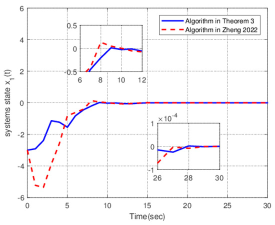
Figure 2.
The response curves of the state .
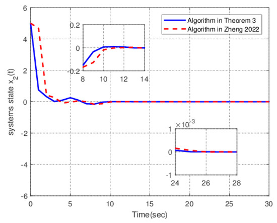
Figure 3.
The response curves of the state .
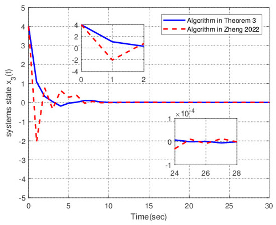
Figure 4.
The response curves of the state .
Figure 2 shows the variation in systems state under two algorithms. The solid line is the response diagram of the systems state under the control action designed by Theorem 4. The dotted line is the response diagram of the systems state under the control action designed by the method given in [20]. It is easy to see from the graph that the solid line converges to 0 faster than the dotted line. The smoothness and overshoot of solid lines are significantly better than those of dotted lines.
Figure 3 shows the variation in systems state under two algorithms. The solid line is the response diagram of the systems state under the control action designed by Theorem 4. The dotted line is the response diagram of the systems state under the control action designed by the method given in [20]. The solid line converges to a small neighborhood of origin within 7 s. The dotted line converges to a small neighborhood of origin only after 10 s, and the convergence speed is slow. The overshoots of the two lines are small, and the amplitude does not exceed 0.1.
Figure 4 shows the variation in systems state under two algorithms. The solid line is the response diagram of the systems state under the control action designed by Theorem 4. The dotted line is the response diagram of the systems state under the control action designed by the method given in [20]. The solid line converges to a small neighborhood of origin within 5 s. The curve is smooth enough, the overshoot is small, and the amplitude does not exceed 0.1. The dotted line converges to a small neighborhood of origin only after 8 s and the convergence speed is slow. The smoothness of the curve is poor, the overshoot is large, and the amplitude reaches 2.
In order to further compare the advantages and disadvantages of the two algorithms, we introduce the following Integral Absolute Error (IAE) performance function to conduct a performance comparison analysis of the systems
After calculation, the IAE performance index function changes, as shown in the following figure.
Figure 5 shows the changes in the IAE performance index of the systems under the two different algorithms. The solid line is the change curve of the IAE performance index of the systems under the algorithm in this paper. The dotted line is the change curve of the IAE performance index of the systems under the algorithm in [20]. The dotted line reaches the peak value 0.081 in 1.9 s. The solid line reaches the peak value 0.061 in 1.7 s. Overall, the slope of the dotted line is relatively large, and the upward speed is fast. The solid line is relatively flat and has good stability.
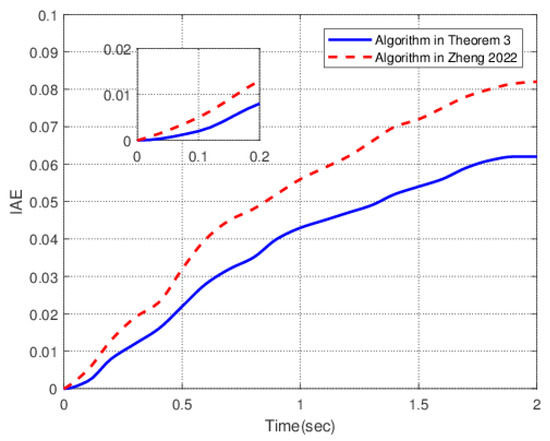
Figure 5.
The change curve of the IAE performance index.
In summary, the fuzzy controller design method proposed in this article is superior to the method presented in [20].
5. Discussion
The contribution of this paper is to design an exponentially stable state observer and dynamic output feedback controller for T-S fuzzy network systems with both state delay and communication delay by using linear matrix inequality method. A less conservative and easy-to-solve method is proposed to reduce the impact of state delay and network communication delay on system performance. The innovation of this paper lies in the design of an exponentially stable state observer and the provision of design conditions for dynamic output feedback control in the form of linear matrix inequalities. It is worth mentioning that our research results can be extended to other types of network systems, such as those with distributed delay, rapidly changing delay, or random delay, which will be our next research work.
6. Conclusions
This paper designs an exponential stable observer and dynamic output feedback control for T-S fuzzy network systems with both state delay and communication delay. The main tasks are as follows: (I) Simultaneously considering the existence of time-varying state delay and network communication delay, T-S fuzzy method is used to establish a mathematical model of the network systems that is more in line with engineering practice. (II) Based on Lyapunov stability theory, an exponential stable state observer is designed by constructing a new Lyapunov functional. (III) Using matrix inequality transformation techniques, the nonlinear stability condition is transformed into a condition in the form of a linear matrix inequality, and a design method for exponential stability control of the systems is given. Unfortunately, the research results are focused on time delay network systems based on T-S models, and studying more complex nonlinear network systems, especially stochastic network systems, will be another topic for us in the future.
Author Contributions
H.Y.: Conceptualization, methodology, software, investigation, writing—original draft, validation. F.G.: software, resources, writing—review and editing, supervision. All authors have read and agreed to the published version of the manuscript.
Funding
This work was supported by the Science and Technology Key Project Henan Province under Grant 242102220109.
Data Availability Statement
The original contributions presented in this study are included in the article. Further inquiries can be directed to the corresponding author.
Conflicts of Interest
The authors declare no conflicts of interest.
References
- Domagoj, T. Stabilizing transmission intervals and delays in nonlinear networked control systems through hybrid-system- with-memory modeling and Lyapunov-Krasovskii arguments. Nonlinear Anal. Hybrid Syst. 2020, 36, 100834. [Google Scholar]
- Song, J.S.; Chang, X.H. H∞ controller design of networked control systems with a new quantization structure. Appl. Math. Comput. 2020, 376, 125070. [Google Scholar] [CrossRef]
- Sun, H.Y.; Sun, J.; Chen, J. Analysis and synthesis of networked control systems with random network-induced delays and sampling intervals. Automatic 2021, 125, 109385. [Google Scholar] [CrossRef]
- Ding, T.F.; Ge, M.F.; Liu, Z.W.; Wang, Y.W.; Karimi, H.R. Lag-bipartite formation tracking of networked robotic systems over directed matrix-weighted. IEEE Trans. Cybern. 2022, 52, 6759–6770. [Google Scholar] [CrossRef] [PubMed]
- Park, J.M. An improved stability criterion for networked control systems with a constant transmission delay. J. Frankl. Inst. 2022, 359, 4346–4365. [Google Scholar] [CrossRef]
- Li, F.H.; Hou, Z.S. Learning-based model-free adaptive control for nonlinear discrete-time networked control systems under hybrid cyber attacks. IEEE Trans. Cybern. 2024, 54, 1560–1570. [Google Scholar] [CrossRef]
- Barmak, B.; Behrooz, R.; Zahra, R. Fuzzy-model-based fault detection for nonlinear networked control systems with periodic access constraints and Bernoulli packet dropouts. Appl. Soft Comput. 2019, 80, 465–474. [Google Scholar]
- Mani, P.; Joo, Y.H. Fuzzy-logic-based event-triggered H∞ control for networked systems and its application to wind turbine systems. Inf. Sci. 2022, 585, 144–161. [Google Scholar] [CrossRef]
- Kundu, A.; Quevedo, D.E. Stabilizing scheduling policies for networked control systems. IEEE Trans. Control Netw. Syst. 2020, 7, 163–175. [Google Scholar] [CrossRef]
- Wang, Y.L.; Yu, S.H. An improved dynamic quantization scheme for uncertain linear networked control systems. Automatica 2018, 92, 244–248. [Google Scholar] [CrossRef]
- Li, Y.J.; Liu, G.P.; Sun, S.L.; Tan, C. Prediction-based approach to finite-time stabilization of networked control systems with time delays and data packet dropouts. Neurocomputing 2019, 329, 320–328. [Google Scholar] [CrossRef]
- Chen, G.; Xia, J.; Zhuang, G. Improved delay-dependent stabilization for a class of networked control systems with nonlinear perturbations and two delay components. Appl. Math. Comput. 2018, 316, 1–17. [Google Scholar] [CrossRef]
- Qi, W.H.; Park, J.H.; Cheng, J.; Chen, X.M. Stochastic stability and L1 -gain analysis for positive nonlinear semi-Markov jump systems with time-varying delay via T-S fuzzy model approach. Fuzzy Sets Syst. 2019, 371, 110–122. [Google Scholar] [CrossRef]
- Wang, L.K.; Lam, H.K. New stability criterion for continuous-time Takagi-sugeno fuzzy systems with time varying delay. IEEE Trans. Cybern. 2019, 49, 1551–1556. [Google Scholar] [CrossRef] [PubMed]
- Yin, Z.; Jiang, X.; Tang, L. On stability and stabilization of T-S fuzzy systems with multiple random variables dependent time-varying delay. Neurocomputing 2020, 412, 91–100. [Google Scholar] [CrossRef]
- Roman, R.C.; Precup, R.E.; Petriu, E.M. Hybrid data-driven fuzzy active disturbance rejection control for tower crane systems. Eur. J. Control 2021, 58, 373–387. [Google Scholar] [CrossRef]
- Chi, R.H.; Li, H.Y.; Shen, D.; Hou, Z.S.; Huang, B. Enhanced P-type control: Indirect adaptive learning from set-point updates. IEEE Trans. Autom. Control 2022, 68, 1600–1613. [Google Scholar] [CrossRef]
- Li, X.H.; Ye, D. Observer-based defense control for networked Takagi-sugeno fuzzy systems against asynchronous DoS attacks. J. Frankl. Inst. 2021, 358, 6136–6160. [Google Scholar] [CrossRef]
- Xu, S.D.; Wen, H.; Wang, X.Y. Observer-based robust fuzzy control of nonlinear networked systems with actuator saturation. ISA Trans. 2022, 123, 122–135. [Google Scholar] [CrossRef]
- Zheng, W.; Zhang, Z.M.; Sun, F.C.; Wen, S.H. Robust stability analysis and feedback control for networked control systems with additive uncertainties and signal communication delay via matrices transformation information method. Inf. Sci. 2022, 582, 258–286. [Google Scholar] [CrossRef]
- Mahmoud, M.S.; Xia, Y.Q.; Zhang, S.X. Robust packet-based nonlinear fuzzy networked control systems. J. Frankl. Inst. 2019, 356, 1502–1521. [Google Scholar] [CrossRef]
- Zheng, W.; Zhang, Z.M.; Lam, H.K.; Sun, F.C.; Wen, S.H. LMIs-based stability analysis and fuzzy-logic controller design for networked systems with sector nonlinearities: Application in tunnel diode circuit. Expert Syst. Appl. 2022, 198, 116627. [Google Scholar] [CrossRef]
- Lian, Z.; Shi, P.; Lim, C.C. Hybrid-triggered interval type-2 fuzzy control for networked systems under attacks. Inf. Sci. 2021, 567, 332–347. [Google Scholar] [CrossRef]
- Cai, X.; Shi, K.B.; She, K.; Zhong, S.M.; Kwon, O.; Tang, Y.Q. Voluntary defense strategy and quantized sample-data control for T-S fuzzy networked control systems with stochastic cyber-attacks and its application. Appl. Math. Comput. 2022, 423, 126975. [Google Scholar] [CrossRef]
- Zhang, D.; Han, Q.; Jia, X. Network-based output tracking control for Takagi–Sugeno fuzzy systems using an event-triggered communication scheme. Fuzzy Sets Syst. 2015, 273, 26–48. [Google Scholar] [CrossRef]
- Su, M.Y.; Che, W.W. Model-free adaptive tracking control for networked control systems under DoS attacks and RTT delays. Int. J. Control Autom. Syst. 2022, 20, 2222–2230. [Google Scholar] [CrossRef]
- Du, Z.; Kao, Y.; Park, J.H.; Zhao, X.; Sun, J.A. Fuzzy event triggered control for nonlinear networked control systems. J. Frankl. Inst. 2022, 359, 2593–2607. [Google Scholar] [CrossRef]
- Li, Z.M.; Chang, X.H.; Xiong, J. Event-based fuzzy tracking control for nonlinear networked systems subject to dynamic quantization. IEEE Trans. Fuzzy Syst. 2022, 31, 941–954. [Google Scholar] [CrossRef]
- Chen, Z.; Zhang, Y.; Kong, Q.; Fang, T.; Wang, J. Observer based H∞ control for persistent dwell-time switched networked nonlinear systems under packet dropout. Appl. Math. Comput. 2022, 415, 126679. [Google Scholar] [CrossRef]
- Pan, Y.N.; Wu, Y.M.; Lam, H.K. Security-based fuzzy control for nonlinear networked control systems with DoS attacks via a resilient event-triggered scheme. IEEE Trans. Fuzzy Syst. 2022, 30, 4359–4368. [Google Scholar] [CrossRef]
- Aslam, M.S.; Radhika, T.; Chandrasekar, A.; Zhu, Q.X. Improved event-triggered-based output tracking for a class of delayed networked T–S fuzzy systems. Int. J. Fuzzy Syst. 2024, 26, 1247–1260. [Google Scholar] [CrossRef]
Disclaimer/Publisher’s Note: The statements, opinions and data contained in all publications are solely those of the individual author(s) and contributor(s) and not of MDPI and/or the editor(s). MDPI and/or the editor(s) disclaim responsibility for any injury to people or property resulting from any ideas, methods, instructions or products referred to in the content. |
© 2025 by the authors. Licensee MDPI, Basel, Switzerland. This article is an open access article distributed under the terms and conditions of the Creative Commons Attribution (CC BY) license (https://creativecommons.org/licenses/by/4.0/).