Rainfall Forecasting Using a BiLSTM Model Optimized by an Improved Whale Migration Algorithm and Variational Mode Decomposition

Abstract

The highly stochastic nature of rainfall presents significant challenges for the accurate prediction of its time series. To enhance the prediction performance of non-stationary rainfall time series, this study proposes a hybrid deep learning forecasting framework—VMD-IWMA-BiLSTM—that integrates Variational Mode Decomposition (VMD), Improved Whale Migration Algorithm (IWMA), and Bidirectional Long Short-Term Memory network (BiLSTM). Firstly, VMD is employed to decompose the original rainfall series into multiple modes, extracting Intrinsic Mode Functions (IMFs) with more stable frequency characteristics. Secondly, IWMA is utilized to globally optimize multiple hyperparameters of the BiLSTM model, enhancing its ability to capture complex nonlinear relationships and long-term dependencies. Finally, experimental validation is conducted using daily rainfall data from 2020 to 2024 at the Xinzheng National Meteorological Observatory. The results demonstrate that the proposed framework outperforms traditional models such as LSTM, ARIMA, SVM, and LSSVM in terms of prediction accuracy. This research provides new insights and effective technical pathways for improving rainfall time series prediction accuracy and addressing the challenges posed by high randomness.

1. Introduction

Multiple intertwined factors, including climate change, topographical heterogeneity, and seasonal variability, influence rainfall forecasting. As a result, rainfall time series often exhibit significant non-stationary characteristics, posing a serious challenge to improving the accuracy of prediction models. To address this issue, existing preprocessing techniques can generally be categorized into two major types: traditional statistical methods and emerging signal decomposition approaches. The traditional methods include differencing [1], logarithmic transformation [2], and exponential smoothing [3]. In contrast, modern signal decomposition techniques, such as Empirical Mode Decomposition (EMD) [4], Ensemble Empirical Mode Decomposition (EEMD) [5], and Variational Mode Decomposition (VMD) [6], have recently gained traction for their ability to transform non-stationary signals into components with more stable characteristics. Among them, VMD has demonstrated significant advantages in both decomposition stability and precision by overcoming the mode mixing problem inherent in EMD through an optimized variational framework. While VMD has been widely applied in fields such as seismic signal processing and energy consumption analysis [7,8], its application in rainfall forecasting remains in the early exploratory stage. Integrating VMD into the preprocessing pipeline for rainfall prediction holds promise for improving forecasting accuracy.

Various methods have been developed for rainfall prediction. For instance, Masum et al. employed an ARIMA model to forecast rainfall and temperature in Chittagong, Bangladesh, from 1953 to 2070 [9], while Karthikeyan et al. utilized an ARMA model to predict non-stationary rainfall data [10]. However, both ARIMA and ARMA are traditional statistical approaches based on linear assumptions, which limit their ability to effectively capture the inherent nonlinear patterns in rainfall data. As a result, these models often suffer from insufficient prediction accuracy when applied to complex hydrological time series.

With the rise of machine learning, the limitations of traditional linear models have gradually been overcome. For example, Hussein et al. applied Support Vector Machines (SVM) for regional rainfall prediction by classifying large-scale precipitation maps [11]. Ma et al. proposed an XGBoost-based flash flood risk assessment method by integrating two input strategies and validating its performance using Least Squares Support Vector Machine (LSSVM), demonstrating its effectiveness [12]. Reddy et al. combined Singular Spectrum Analysis (SSA) as a data preprocessing technique with supervised learning models such as Least Squares Support Vector Regression (LSSVR) and Random Forest (RF) to enhance rainfall prediction reliability [13]. However, these machine learning approaches often fail to capture the dynamic characteristics inherent in time series data adequately.

In recent years, deep learning techniques have garnered significant attention due to their powerful capabilities in sequence modeling. Ma et al. employed a multimodal recurrent neural network (MM-RNN) for rainfall prediction [14]. As a classical time series model, RNN can capture temporal dependencies within sequences; however, it is prone to gradient vanishing or exploding in long-term predictions, leading to the “forgetting” of critical earlier information. To address this, Poornima et al. utilized the Long Short-Term Memory (LSTM) model for rainfall estimation [15], and Salehin et al. applied LSTM to assess rainfall and improve crop yield forecasting [16]. By introducing input, forget, and output gates, LSTM effectively regulates the flow and retention of information, thereby mitigating the long-term dependency issues of RNNs and demonstrating superior temporal modeling performance in rainfall forecasting tasks. Nevertheless, conventional LSTM networks rely solely on unidirectional information flow, which limits their ability to fully capture global sequence trends and variation patterns.

To address these limitations, Xie et al. employed a Bidirectional Long Short-Term Memory (BiLSTM) model to impute temperature data [17]. At the same time, Siami-Namini et al. conducted a comparative analysis of LSTM and BiLSTM models in time series forecasting tasks [18]. BiLSTM integrates both forward and backward LSTM units, allowing it to capture information from both past and future contexts within the sequence. This dual-directional structure significantly enhances the model’s ability to comprehend and retain complex sequence patterns. Empirical studies have demonstrated that BiLSTM outperforms conventional LSTM models across various time series prediction scenarios [19]. Accordingly, this study adopts BiLSTM as the baseline model for rainfall forecasting.

In BiLSTM models, hyperparameters have a substantial impact on predictive performance. Studies have shown that the influence of hyperparameters on deep learning models often exceeds that of the model architecture itself [20]. The core objective of hyperparameter optimization is to define a search space comprising the tunable hyperparameters and their value ranges, and then use an optimization algorithm to explore this space in search of the optimal configuration [21]. However, due to the large number of hyperparameters and the broad range of possible values for each, the search space contains an enormous number of parameter combinations that must be evaluated individually to identify the best solution [22]. This renders hyperparameter optimization a challenging task in deep learning applications. In the context of BiLSTM-based rainfall forecasting, hyperparameters can generally be categorized into two groups: (1) structural hyperparameters, such as the number of units per BiLSTM layer and the number of stacked BiLSTM layers, and (2) training-related hyperparameters, such as the learning rate (i.e., the step size for parameter updates during training), dropout rate (which determines the proportion of neurons randomly dropped during training), maximum number of epochs, optimization algorithm, and loss function [23,24,25]. Due to the vast number of hyperparameters and the size of their respective search spaces, optimizing all of them simultaneously is computationally expensive. Therefore, this study focuses on optimizing the three most critical hyperparameters that have the most significant impact on BiLSTM performance.

In traditional studies, hyperparameters are often manually configured based on the researcher’s experience, a highly subjective approach that makes it challenging to ensure globally optimal solutions [26]. Against this backdrop, automated hyperparameter optimization methods have gradually become a research focus. Currently, the mainstream approaches include Grid Search [27], Random Search [28], and Bayesian Optimization [29]. Grid Search is straightforward and intuitive but suffers from high computational costs. Random Search reduces computational burden but lacks stability and consistency. Bayesian Optimization, on the other hand, constructs a probabilistic model to guide the search process effectively. However, it is prone to getting trapped in local optima in high-dimensional and complex search spaces.

In recent years, Swarm Intelligence (SI) optimization algorithms have garnered attention due to their robust global search capabilities and strong performance. They have been successfully applied in domains such as wind speed forecasting, image recognition, and medical diagnosis [30,31,32]. However, their application in rainfall prediction remains relatively limited. SI algorithms are a class of heuristic optimization methods inspired by collective behaviors in nature—such as bird flocking and fish schooling—and are designed to find global or near-global solutions through collaborative search strategies [33]. Currently, mainstream SI algorithms include the Harris hawks optimization (HHO), Sine cosine algorithm (SCA), Grey wolf optimizer (GWO), Elk herd optimization (EHO), Butterfly optimization algorithm (BOA), Whale optimization algorithm (WOA), Particle swarm optimization (PSO), and Differential evolution (DE) [34,35,36,37,38,39,40,41]. Although a wide range of SI algorithms has been developed, the “No Free Lunch” theorem suggests that no single optimization algorithm is universally superior for all types of problems [42]. In other words, an algorithm that performs well on one class of problems may not perform as well on others [43]. Therefore, enhancing existing algorithms to improve their effectiveness in solving specific types of problems remains a valuable direction for research.

The Whale Migration Algorithm (WMA), proposed by Ghasemi et al. in 2025 [44], is inspired by the cooperative and migratory behavior of humpback whales. It demonstrates strong global search capability, fast convergence speed, and excellent adaptability and robustness. Previous studies have shown that WMA outperforms several mainstream metaheuristic algorithms, including HHO, SCA, GWO, EHO, BOA, WOA, PSO, and DE, across various benchmark test functions. Despite its competitive performance, WMA tends to encounter issues such as “clustering” or “biased distribution” during the initial population generation phase, which may cause the search process to fall into local optima. To enhance population diversity and global exploration ability, this study incorporates a logistic map-based chaotic initialization strategy [45], which exhibits ergodic and stochastic properties. Furthermore, the original WMA lacks an explicit elitism mechanism, which may result in the loss of the current best solution during iterative updates. To improve convergence stability and solution accuracy, an elitism preservation strategy [46] is also introduced. Based on these enhancements, we propose an Improved Whale Migration Algorithm (IWMA). To validate the effectiveness of IWMA, comprehensive experiments were conducted on a suite of standard benchmark test functions, and the performance was compared against nine representative optimization algorithms, including HHO, SCA, GWO, EHO, BOA, WOA, PSO, DE, and the original WMA.

The paper proposes a novel hybrid deep learning prediction framework—VMD-IWMA-BiLSTM—which comprehensively utilizes Variational Mode Decomposition (VMD), Improved Whale Migration Algorithm (IWMA), and Bidirectional Long Short-Term Memory Network (BiLSTM) to achieve accurate modeling of rainfall data.

2. Materials and Methods

This study proposes a novel VMD-IWMA-BiLSTM framework for rainfall forecasting and optimization. The framework consists of three core modules. First, Variational Mode Decomposition (VMD) is introduced as a signal decomposition technique to handle non-stationary data, which serves as a preprocessing step for the rainfall series. Second, the Bidirectional Long Short-Term Memory (BiLSTM) network is employed as the central deep learning model to perform the forecasting task. Third, the Improved Whale Migration Algorithm (IWMA) is utilized as a swarm intelligence-based optimization tool to optimize three key hyperparameters of the BiLSTM network. The following sections provide a detailed introduction to the signal decomposition method, the forecasting model, and the optimization algorithm, respectively.

2.1. VMD

Variational Mode Decomposition (VMD) is a novel signal decomposition method proposed by Dragomiretskiy and Zosso in 2014 [6]. In contrast to Empirical Mode Decomposition (EMD) and its variants, Variational Mode Decomposition (VMD) eliminates the dependence on local extrema and envelope interpolation by formulating a constrained optimization problem in the frequency domain. Through a variational optimization framework, VMD enables robust and adaptive signal decomposition. This approach provides enhanced parameter controllability and algorithmic stability, effectively overcoming the mode mixing issue frequently encountered in conventional decomposition methods.

First, a variational model is constructed by assuming that the rainfall data are decomposed into $\mathrm{K}$ intrinsic mode components. The model imposes a constraint that the sum of all components equals the original signal. The corresponding constrained variational formulation is given in Equation (1):

$$\begin{array}{l}{\min }_{\{u_k,{{\displaystyle \omega }}_k\}}\left\{{\displaystyle \sum _k{\left|{\sigma }_l\left[\left(\delta (t)+\frac{j}{\pi t}\right)\ast u_k(t)\right]e^{-j{\omega }_{k}t}\right|}_2^2}\right\}\\ {\displaystyle \sum _k{u}_k}=f(t)n\end{array}$$

(1)

Here, {$u_k$} is the kth modal component, {${\omega }_k$} is the central frequency of the kth mode, $\delta \left(t\right)$ is the Dirac delta function, and * denotes the convolution operator.

Subsequently, the formulated variational problem is addressed by introducing Lagrange multipliers $\lambda$, thereby converting the original constrained problem into an unconstrained variational form. The corresponding augmented Lagrangian expression is presented in Equation (2):

$$\begin{array}{l}L(\{u_k\},\{{\omega }_k\},\lambda )=\alpha {\displaystyle \sum _k{‖{\sigma }_l\left[\left(\delta (t)+\frac{j}{\pi t}\right)\ast u_k(t)\right]e^{-j{\omega }_{k}t}‖}_2^2}\\ +{‖f(t)-{\displaystyle \sum _k{u}_k}(t)‖}_2^2+〈\lambda \left(t\right),f(t)-{\displaystyle \sum _k{u}_k}(t)〉\end{array}$$

(2)

where α is the quadratic penalty factor for reducing the interference of Gaussian noise and $\lambda \left(t\right)$ represents the Lagrange operator.

The modal components and their corresponding center frequencies are obtained through the Alternating Direction Method of Multipliers (ADMM) and Fourier isometric transformation optimization. Among them, the center frequency is constrained within the range [0,+∞), which ensures strict compliance with the requirements of isometric transformation optimization in VMD. The main procedure is as follows: Leveraging the energy-equidistant property of isometric transformation, the VMD optimization problem is mapped onto a uniformly distributed frequency space, thereby ensuring minimal spectral overlap among modes. This improves the accuracy of mode separation by mitigating mode aliasing and ensures that each ${\omega }_k$ is confined to the dominant frequency band of the actual signal, avoiding energy leakage and spectral redundancy. To this end, for low-frequency modes ($\omega \approx 0$), the center frequency update function ${\omega }_k \to {\omega }_k^{’}$ adopts a “weighted dual-boosting” strategy to penalize non-physical negative frequency values, ensuring energy-concentrated characteristics. Accordingly, when $\omega >0$ (non-zero center frequency), the update proceeds along the regular optimization direction, whereas for $\omega \le 0$, a reconstruction operation is introduced, as detailed in Equations (3)–(5).

$${\widehat{u}}_k^{n+1}(\omega )={\displaystyle \frac{\widehat{f}(\omega )-{\displaystyle \sum _{i\ne k}{u}_i}(\omega )+\widehat{\lambda }(\omega )/2}{1+2\alpha {(\omega -{\omega }_k)}^2}}$$

(3)

$${\omega }_k^{n+1}={\displaystyle \frac{{\displaystyle {\int }_0^{\infty }\omega }{\left|{\widehat{u}}_k^{n+1}(\omega )\right|}^{2}d\omega }{{\displaystyle {\int }_0^{\infty }{\left|{\widehat{u}}_k^{n+1}(\omega )\right|}^2}d\omega }}$$

(4)

$${\widehat{\lambda }}_k^{n+1}(\omega )={\widehat{\lambda }}_k^n(\omega )+\gamma \left(\widehat{f}(\omega )-{\displaystyle \sum _k{\widehat{u}}_k^{n+1}}(\omega )\right)$$

(5)

Among these variables, ${\widehat{u}}_k^{n+1}$, $u_i\left(\omega \right)$, and $\widehat{f}\left(\omega \right)$ represent the Fourier transforms of $u_k^{\left(n+1\right)}\left(t\right)$, $u_i\left(t\right)$, and $f\left(t\right)$, respectively. The constraints are applied until the constraint conditions are satisfied in Equation (6) is met:

$${\displaystyle \sum _{k=1}^K\left(\frac{\Vert {\widehat{u}}_k^{(n+1)}-{\widehat{u}}_k^n{\Vert }_2^2}{\Vert {\widehat{u}}_k^n{\Vert }_2^2}\right)}<\in$$

(6)

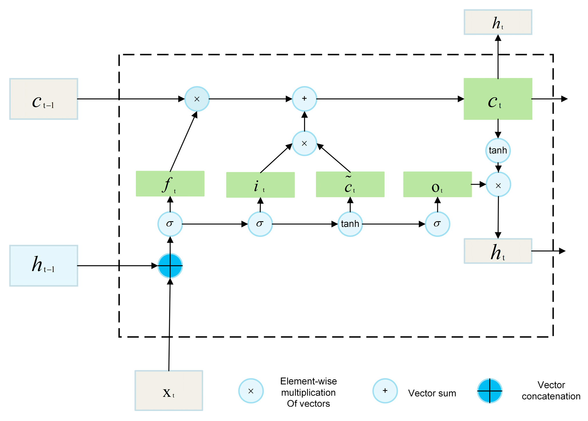
2.2. Rainfall Prediction Model: BiLSTM

The BiLSTM network used in this study is a variant of the Long Short-Term Memory (LSTM) model. It introduces three gating mechanisms—forget gate, input gate, and output gate—to regulate the flow of information, thereby enabling effective modeling of time series data. Specifically, the forget gate determines how much of the previous cell state should be discarded, the input gate controls how much of the current input should be added to the cell state, and the output gate decides how much information from the cell state should be passed to the current hidden state. The structure of the LSTM unit is illustrated in Figure 1.

The calculation of LSTM is shown in Equations (7)–(12):

$$f_t=\sigma (w_f\times h_{t-1}+u_f\times x_t+b_f)$$

(7)

$$i_t=\sigma (w_i\times h_{t-1}+u_i\times x_t+b_i)$$

(8)

$${\tilde{c}}_t=\tanh (w_c\times h_{t-1}+u_c\times x_t+b_c)$$

(9)

$$c_t=f_t\odot c_{t-1}+i_t\odot {\tilde{c}}_t$$

(10)

$$o_t=\sigma (w_o\times h_{t-1}+u_o\times x_t+b_o)$$

(11)

$$h_t=o_t\odot \tanh (c_t)$$

(12)

Among them, represents the forget gate, represents the input gate, represents the output gate, the new state is the additional new information learned at the current moment t, and the current information is how much information is extracted from previous moments plus how much information is extracted from the current moment.

The BiLSTM unit is composed of a forward LSTM and a backward LSTM, which extract temporal features from the input sequence in the forward and reverse time directions, respectively. Compared with the standard LSTM, BiLSTM can capture temporal dependencies more comprehensively through its bidirectional information flow mechanism, thereby significantly enhancing its sequence modeling capability. Therefore, BiLSTM is adopted in this study as the core unit of the prediction model. Its specific structure is shown in Figure 2.

2.3. IWMA

Since the BiLSTM model involves several critical hyperparameters that significantly influence its performance, it is necessary to employ optimization algorithms to automatically determine the optimal parameter combination. To this end, this study introduces an improved Whale Migration Algorithm (IWMA) to optimize the BiLSTM model. Based on the original Whale Migration Algorithm (WMA), IWMA integrates a chaotic initialization strategy using logistic mapping and an elite retention mechanism, thereby enhancing search diversity and convergence stability. The remainder of this section introduces the basic principles of the original WMA and details the improvements incorporated in the proposed IWMA.

2.3.1. The Original WMA

The Whale Migration Algorithm (WMA) was proposed by Ghasemi et al. in 2025 [44]. Inspired by the migratory behavior of humpback whale groups, the algorithm innovatively introduces a “leader–follower” dynamic mechanism to replace the individual hunting-based optimization strategy used in conventional algorithms such as the Whale Optimization Algorithm (WOA). As illustrated in Figure 3, the fundamental mechanism of WMA includes a “move toward the nearest solution” strategy for inexperienced individuals and a “guided exploration” strategy for experienced individuals. During the iteration process, the algorithm determines the update method for each individual based on its experience level, thereby achieving an optimization dynamic that balances “local exploitation” and “global exploration”, enhancing both convergence accuracy and search efficiency. The overall WMA process can be divided into three stages: population initialization, the follower phase for inexperienced individuals, and the exploration phase for experienced individuals. The strategies for each stage are detailed as follows.

• Population initialization phase

In the initialization phase, WMA first generates an initial population consisting of n whale individuals, where each individual is represented as a D-dimensional solution vector. The initialization is carried out using a uniform random strategy:

$$W_i = L + \mathrm{r}\mathrm{a}\mathrm{n}\mathrm{d}\left(1,D\right) \odot \left(U - L\right),i = \mathrm{1,2},\dots ,N_{\mathrm{p}\mathrm{o}\mathrm{p}}$$

(13)

where $L$ and $U$ denote the lower and upper bounds of the search space, respectively; rand(1, D) represents uniformly distributed random numbers in the interval [0, 1]; and $\odot$ denotes the Hadamard product. This step is intended to provide diverse initial solutions for the algorithm.

2.

Following Phase for Inexperienced Whales

In this stage, two key mechanisms are employed: movement of less-experienced whales (juveniles) toward the nearest solution, and guided movement under the leadership of more experienced individuals. Specifically, in each iteration, the top-performing individuals are selected based on fitness values to form the leader set. The central position of this leader group is defined as follows:

$$W_{\mathrm{m}\mathrm{e}\mathrm{a}\mathrm{n}} = {\displaystyle \frac{1}{N_L}}\sum _{i = 1}^{N_L}{W}_i$$

(14)

where $W_i$ denotes the position of the i-th leader individual, and ${\mathrm{N}}_{\mathrm{L}}$ represents the number of leader individuals.

For individuals ranked lower in the population (i.e., non-leader individuals), an imitation mechanism is adopted for the update strategy: their positions are updated by imitating the position of the previous whale, the mean position of the leaders ${\mathrm{W}}_{\mathrm{m}\mathrm{e}\mathrm{a}\mathrm{n}}$, and the current best position ${\mathrm{W}}_{\mathrm{B}\mathrm{e}\mathrm{s}\mathrm{t}}$. The update formula is as follows:

$$\begin{array}{ll}{W}_i^{\mathrm{n}\mathrm{e}\mathrm{w}} =& W_{\mathrm{m}\mathrm{e}\mathrm{a}\mathrm{n}} + \mathrm{r}\mathrm{a}\mathrm{n}\mathrm{d}\left(1,D\right) \odot (W_{i-1} - W_i)\\ & + \mathrm{r}\mathrm{a}\mathrm{n}\mathrm{d}\left(1,D\right) \odot \left(W_{\mathrm{B}\mathrm{e}\mathrm{s}\mathrm{t}}-W_{\mathrm{m}\mathrm{e}\mathrm{a}\mathrm{n}}\right),i = N_L + 1,\dots ,N_{\mathrm{p}\mathrm{o}\mathrm{p}}\end{array}$$

(15)

• ${\mathrm{W}}_{\mathrm{i}}^{\mathrm{n}\mathrm{e}\mathrm{w}}$ denotes the new position of the i-th non-leader individual;
• rand(1,D) represents a uniformly distributed random number within the interval [0, 1];
• $\odot$ denotes the Hadamard product;
• ${\mathrm{W}}_{\mathrm{B}\mathrm{e}\mathrm{s}\mathrm{t}}$ is the current best solution in the population;
• ${\mathrm{N}}_{\mathrm{p}\mathrm{o}\mathrm{p}}$ is the total population size, and ${\mathrm{N}}_{\mathrm{L}}$ is the number of leader individuals.

3.

Exploration by Experienced Whales

The top ${\mathrm{N}}_{\mathrm{L}}$ whales in the ranking are considered “leaders”. They guide the entire population to explore new regions through perturbation-based wide-range search. The position update is defined as follows:

$$\begin{array}{ll}{W}_i^{\mathrm{n}\mathrm{e}\mathrm{w}} =& W_i + r_1 \odot L\\ & +{ r}_1 \odot r_2 \odot \left(U - L\right), i =\mathrm{1,2},\dots ,N_L\end{array}$$

(16)

• $r1,r2$: random vectors with values in the interval [0, 1];
• $L,U$: the lower and upper bounds of the search space.

2.3.2. Proposed IWMA

Although the original Whale Migration Algorithm (WMA) demonstrates notable advantages in terms of global search capability, convergence speed, and robustness, it also presents several limitations. Specifically, the algorithm is prone to issues such as “clustering” or “biased distribution” during the initial population generation phase, which may cause the search process to fall into local optima. Moreover, the original WMA lacks an explicit elitism mechanism, making it possible to lose the current best solutions during iterative updates. To address these issues, we incorporate two enhancement mechanisms into the original WMA. The details of these improvements are presented below.

• Chaotic Mapping Mechanism

To enhance the population diversity and solution space coverage capability of the Whale Migration Algorithm (WMA) during the early stages of the search process, this study adopts a logistic chaotic sequence for population initialization. Compared to the traditional uniform random initialization, which may result in uneven distribution and premature convergence, chaotic mapping—owing to its properties of ergodicity, sensitivity to initial conditions, and pseudo-randomness—can effectively improve the global exploration ability in the initial phase of the algorithm. In this work, the adopted logistic map is formulated as follows:

$$\begin{array}{c}{x}_{n+1 }= r \cdot x_n\left(1 - x_n\right), r = 4, x_n \in \left(\mathrm{0,1}\right)\end{array}$$

(17)

During the initialization of the population, the chaotic sequence generated by the logistic map is mapped to the search space:

$$W_i = L + x_i \cdot \left(U - L\right), i = \mathrm{1,2},\dots ,N$$

(18)

where ${\mathrm{x}}_{\mathrm{i}}$ represents the chaotic sequence generated by the logistic map, and $L$ and $U$ denote the lower and upper bounds of the decision variables, respectively. Experimental results show that applying chaotic initialization enables a more uniform population coverage, significantly improving the quality of early-stage searches and providing a better convergence foundation for subsequent iterations.

2.

Elite Retention Mechanism

To further enhance the algorithm’s ability to maintain the global optimum and improve convergence accuracy, this study introduces an elite retention strategy. Specifically, in each iteration, the currently best-performing individual (referred to as the elite) is preserved and used to guide the update of other individuals during the evolutionary process. The detailed implementation is as follows: during each population update, the individual with the best fitness value is embedded into the update formula for non-leader individuals, serving as a guide to direct their evolution. The specific update strategy is given by the following:

$$W_i^{\mathrm{n}\mathrm{e}\mathrm{w}} ={ W}_{\mathrm{m}\mathrm{e}\mathrm{a}\mathrm{n}} + {\mathbf{r}}_1 \odot \left(W_{i - 1} - W_i\right) + {\mathbf{r}}_2 \odot \left(W_{\mathrm{E}\mathrm{l}\mathrm{i}\mathrm{t}\mathrm{e}} - W_{\mathrm{m}\mathrm{e}\mathrm{a}\mathrm{n}}\right), i >{ N}_L$$

(19)

• ${\mathrm{W}}_{\mathrm{m}\mathrm{e}\mathrm{a}\mathrm{n}}$: the mean position of the current leader individuals.
• ${\mathrm{W}}_{\mathrm{E}\mathrm{l}\mathrm{i}\mathrm{t}\mathrm{e}}$: the position of the globally optimal individual.
• ${\mathrm{r}}_1,{\mathrm{r}}_2\in {\left[\mathrm{0,1}\right]}^{\mathrm{D}}$: random vectors within the range [0, 1] in D-dimensional space.

The proposed strategy not only enhances the stability of the algorithm but also significantly improves its local exploitation capability in the middle and later stages of the search. By preventing the optimal solution from being forgotten or replaced by inferior ones, it further accelerates the convergence speed and improves the solution accuracy.

The final proposed IWMA flowchart is illustrated in Figure 4, where the components highlighted in purple represent our improvements.

3. Results and Discussion

3.1. IWMA Performance Verification Experiments

In this section, a series of experiments are conducted to evaluate the optimization performance of the proposed Improved Whale Migration Algorithm (IWMA), focusing on its exploitation capability, exploration capability, and ability to avoid local optima. The experimental design includes both ablation studies and comparative analyses with mainstream metaheuristic algorithms. All experiments are performed under the same hardware environment to ensure a fair comparison. Specifically, the experiments are conducted on a computer equipped with a 12th Gen Intel^® Core™ i5-12500H 12-core processor and an NVIDIA GeForce RTX 4060 GPU with 8 GB of VRAM (Manufacturer: Mechanical Revolution, City: Beijing, China, Country: China). To maintain consistency across tests, all algorithms are configured with the same parameters: the maximum number of iterations (T) is set to 500, and the population size (n) is set to 30.

3.1.1. Benchmark Functions

To comprehensively evaluate the optimization performance of the proposed Improved Whale Migration Algorithm (IWMA), we conducted comparative experiments using 29 benchmark functions selected from the CEC2017 test suite [47]. These 29 functions are categorized into four types: F1–F3 are unimodal benchmark functions used to assess the algorithm’s exploitation capability (note that the original F2 was removed by the official committee, resulting in an adjusted range of F1–F3); F4–F10 are multimodal benchmark functions designed to evaluate exploration capability; F11–F20 are hybrid functions used to test adaptability in heterogeneous problem landscapes; and F21–F30 are composition functions intended to evaluate the algorithm’s ability to avoid local optima. “Range” denotes the boundary constraints of the decision variables, and “F(min)” represents the global optimum. The CEC2017 benchmark functions are summarized in

Table 1. Benchmark functions of CEC 2017 [48].

Type	No.	Functions	Fi * = Fi (x*)1
Unimodal Functions	1	Shifted and Rotated Bent Cigar Function	100
	3	Shifted and Rotated Zakharov Function	200
Simple Multimodal Functions	4	Shifted and Rotated Rosenbrock’s Function	300
	5	Shifted and Rotated Rastrigin’s Function	400
	6	Shifted and Rotated Expanded Scaffer’s F6 Function	500
	7	Shifted and Rotated Lunacek Bi_Rastrigin Function	600
	8	Shifted and Rotated Non-Continuous Rastrigin’s Function	700
	9	Shifted and Rotated Levy Function	800
	10	Shifted and Rotated Schwefel’s Function	900
Hybrid Functions	11	Hybrid Function 1 (N = 3)	1000
	12	Hybrid Function 2 (N = 3)	1100
	13	Hybrid Function 3 (N = 3)	1200
	14	Hybrid Function 4 (N = 4)	1300
	15	Hybrid Function 5 (N = 4)	1400
	16	Hybrid Function 5 (N = 4)	1500
	17	Hybrid Function 6 (N = 5)	1600
	18	Hybrid Function 6 (N = 5)	1700
	19	Hybrid Function 6 (N = 5)	1800
	20	Hybrid Function 6 (N = 6)	1900
Composition Functions	21	Composition Function 1 (N = 3)	2000
	22	Composition Function 2 (N = 3)	2100
	23	Composition Function 3 (N = 4)	2200
	24	Composition Function 4 (N = 4)	2300
	25	Composition Function 5 (N = 5)	2400
	26	Composition Function 6 (N = 5)	2500
	27	Composition Function 7 (N = 6)	2600
	28	Composition Function 8 (N = 6)	2700
	29	Composition Function 9 (N = 3)	2800
	30	Composition Function 10 (N = 3)	2900

Fi *: the optimal solution function valued.

.

In this experimental section, to reduce the impact of randomness, each algorithm was independently executed 30 times on every benchmark test function, and the resulting outcomes were recorded. To systematically evaluate the overall performance of each algorithm across multiple benchmark functions, the Friedman rank test was employed to rank and statistically analyze the optimization results. This method provides a robust statistical basis for comparing the relative performance of multiple algorithms over a range of problems, enabling a comprehensive and objective assessment of their strengths and weaknesses.

3.1.2. Ablation Analysis of the IWMA

Building upon the original Whale Migration Algorithm (WMA), this study introduces a chaotic mapping strategy and an elite retention mechanism to propose an improved variant, namely IWMA. To evaluate the effectiveness of these enhancements, ablation experiments were designed to systematically assess the performance of various WMA variants incorporating different combinations of these mechanisms.

Table 2. Different variants of WMA incorporating two mechanisms.

Model	CM 1	ERM 2
IWMA	1	1
CWMA	1	0
EWMA	0	1
WMA	0	0

¹ CM: Chaotic Mapping Strategy. ² ERM: Elite Retention Strategy.

presents the WMA variants, where “1” indicates the inclusion of a specific mechanism and “0” denotes its exclusion. All algorithmic variants were executed on the 29 benchmark functions from the aforementioned CEC2017 suite. The experiments aim to comprehensively analyze the individual contributions and synergistic effects of each mechanism on the overall performance of the algorithm.

The experimental results are presented in Table 2. Here, Avg denotes the average rank value of each algorithm across the 29 benchmark functions based on the Friedman test. A lower Avg value indicates better overall optimization performance. The column “+/−/=” represents the number of functions on which the proposed IWMA achieves better, worse, or comparable performance relative to other WMA variants. Rank indicates the final comprehensive ranking of each algorithm among all compared variants.

As shown in the results of

Table 3. Ablation experiment results.

Algorithm	Rank	+/−/=	Avg
IWMA	1	~	2.3103
CWMA	2	13/12/1	2.3793
EWMA	3	12/16/1	2.6207
WMA	4	13/12/1	2.6897

, the baseline version of the WMA algorithm performs the worst among all variants. The incorporation of either the chaotic mapping strategy or the elitism strategy can improve the optimization performance to varying degrees. Among all tested algorithms, IWMA, which integrates both strategies, ranks first overall. This indicates that the combination of chaotic initialization and elitism significantly enhances the algorithm’s global search capability and convergence performance, thereby effectively improving its overall optimization ability.

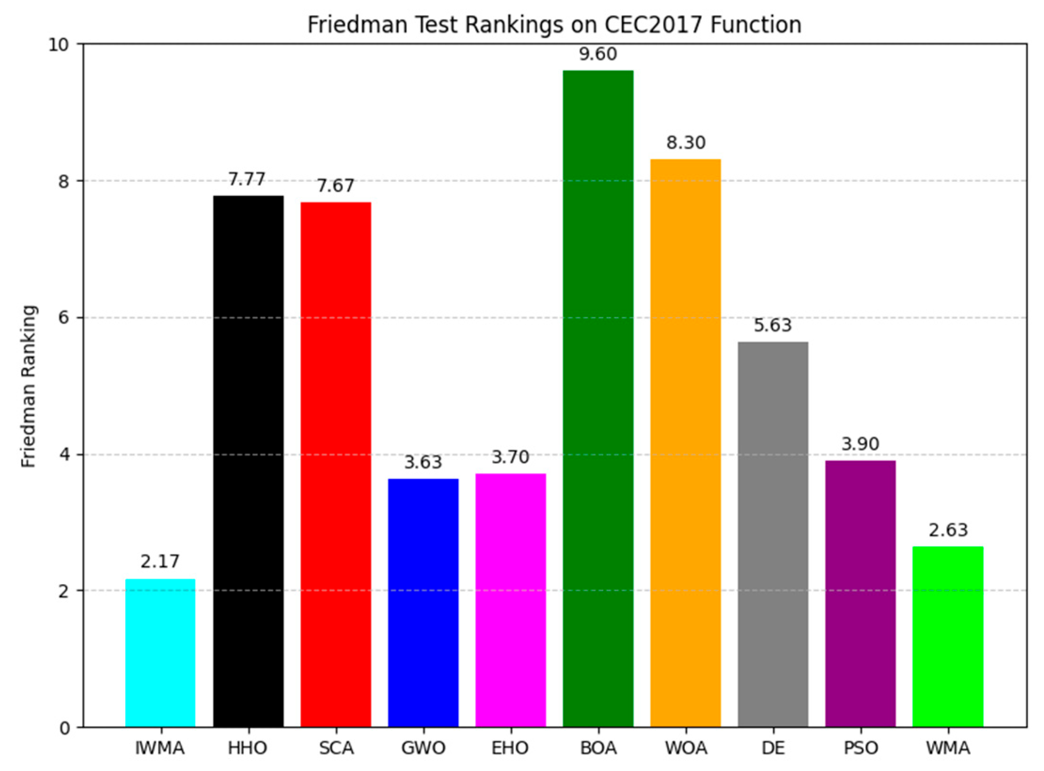
3.1.3. Comparison with Other Algorithms

To further verify the optimization performance of the proposed IWMA algorithm, this study conducted comparative experiments between IWMA, the original WMA algorithm, and eight other representative and widely used metaheuristic algorithms. The selected benchmark algorithms are as follows:

• Harris hawks optimization (HHO) [38];
• Sine cosine algorithm (SCA) [39];
• Grey wolf optimization (GWO) [40];
• Elk herd optimization (EHO) [41];
• Butterfly optimization algorithm (BOA) [42];
• Whale optimization algorithm (WOA) [43];
• Particle swarm optimization (PSO) [44];
• Differential evolution (DE) [45].

The parameter settings of the aforementioned comparison algorithm are shown in

Table 4. Parameter configurations of comparison algorithms.

Algorithm	Parameter	Value
HHO	Escape energy (E), Random number (q, r)	E ∈ (−1–1); q, r ∈ (0,1)
SCA	Convergence parameter spiral factor (a)	a = 2
GWO	Area vector (a), random vector (r1, r2)	A ∈ [0, 2], r1 ∈ [0, 1], r2 ∈ [0, 1]
EHO	Male ratio (br)	br ϵ (0–1)
BOA	Perception factor (c)	c ϵ (0.01–0.1)
WOA	Convergence factor decay rate (a)	a ϵ (2 → 0)
PSO	Population size of the particle swarm	α ϵ (20–1000)
DE	Scaling factor (F), Crossover probability (CR)	F ϵ (0–2], CR ϵ [0–1]
WMA	Population size (N), Number of leaders (NL)	N ϵ (20–100), NL ϵ (10–50)

:

To ensure fairness in the experiments, all algorithms were executed under the same computational environment, with the maximum number of iterations set to 500 and a population size of 30. To mitigate the impact of randomness on the experimental outcomes, each algorithm was independently run 30 times on each benchmark test function, and the average value (Aver) and standard deviation (Std) of the results were calculated.

Table 5. Experimental results on 29 benchmark functions (optimal values are shown in boldface).

Fun	F1		F3		F4
	Aver	Std	Aver	Std	Aver	Std
IWMA	3.8335E+03	4.2917E+03	4.5676E+04	1.3383E+04	4.9064E+02	2.1045E+01
HHO	4.6203E+08	2.8176E+08	5.6934E+04	7.3345E+03	6.8264E+02	7.5893E+01
SCA	2.0577E+10	3.1811E+09	8.7978E+04	2.0971E+04	3.5622E+03	1.2615E+03
GWO	2.3986E+09	1.5824E+09	6.3014E+04	1.2302E+04	7.1221E+02	3.0209E+02
EHO	2.7460E+04	6.2361E+04	2.2317E+08	1.3346E+05	5.1184E+02	4.2300E+01
BOA	3.6896E+10	7.5074E+09	1.4765E+05	4.8241E+04	1.2544E+04	2.6969E+03
WOA	6.5862E+09	2.8032E+09	2.7092E+05	6.0351E+04	1.3645E+03	3.8047E+02
PSO	9.6025E+08	1.1254E+09	6.6689E+04	3.0171E+04	6.9417E+02	3.3474E+02
DE	1.1514E+08	5.0998E+07	1.9832E+05	2.3148E+04	5.6293E+02	2.3962E+01
WMA	8.2757E+03	7.8386E+03	6.1679E+04	2.1791E+04	4.8691E+02	1.6544E+01
	F5		F6		F7
	Aver	Std	Aver	Std	Aver	Std
IWMA	6.1811E+02	5.3252E+01	6.2289E+02	1.0344E+01	8.9391E+02	6.4040E+01
HHO	7.7268E+02	2.8107E+01	6.6673E+02	6.5391E+00	1.3244E+03	6.1795E+01
SCA	8.2804E+02	2.6270E+01	6.6291E+02	5.7395E+00	1.2241E+03	5.3127E+01
GWO	6.1629E+02	3.2591E+01	6.1262E+02	6.0461E+00	8.9891E+02	6.3787E+01
EHO	6.3614E+02	6.3391E+01	6.1997E+02	9.3679E+00	9.3030E+02	7.8652E+01
BOA	8.4816E+02	2.8787E+01	6.8019E+02	9.3301E+00	1.2631E+03	7.9684E+01
WOA	8.6193E+02	8.0098E+01	6.8101E+02	8.2975E+00	1.3248E+03	8.0341E+01
PSO	6.2439E+02	3.1687E+01	6.1707E+02	8.2960E+00	8.7893E+02	4.3155E+01
DE	7.3265E+02	1.7138E+01	6.0717E+02	1.0704E+00	9.8986E+02	1.7707E+01
WMA	6.1073E+02	5.1076E+01	6.2055E+02	6.7917E+00	9.2189E+02	5.9488E+01
	F8		F9		F10
	Aver	Std	Aver	Std	Aver	Std
IWMA	9.2511E+02	5.0289E+01	3.1146E+03	1.4248E+03	6.6263E+03	1.4733E+03
HHO	9.8562E+02	2.1213E+01	8.5077E+03	1.1114E+03	6.1629E+03	7.8103E+02
SCA	1.1009E+03	2.3298E+01	8.1538E+03	1.4530E+03	8.9109E+03	3.7081E+02
GWO	8.9907E+02	1.9437E+01	2.6117E+03	9.8134E+02	5.7143E+03	1.5692E+03
EHO	9.2112E+02	5.4542E+01	4.6601E+03	2.6534E+03	8.1383E+03	1.6801E+03
BOA	1.0875E+03	3.4643E+01	8.4363E+03	1.8711E+03	8.2623E+03	2.6840E+02
WOA	1.0754E+03	4.6075E+01	1.1753E+04	3.9656E+03	7.6494E+03	7.5031E+02
PSO	9.1193E+02	2.3463E+01	3.5110E+03	2.2083E+03	4.4821E+03	7.2567E+02
DE	1.0397E+03	1.4250E+01	5.1060E+03	1.0360E+03	8.1185E+03	3.6845E+02
WMA	9.3006E+02	6.2443E+01	3.0402E+03	1.3284E+03	7.6698E+03	4.1130E+02
	F11		F12		F13
	Aver	Std	Aver	Std	Aver	Std
IWMA	1.2482E+03	5.5580E+01	5.2486E+05	1.1992E+06	1.1842E+04	1.2110E+04
HHO	1.5881E+03	1.8010E+02	8.8699E+07	7.5546E+07	1.0541E+06	5.9189E+05
SCA	4.3086E+03	1.4446E+03	2.6397E+09	6.8462E+08	1.2108E+09	8.5282E+08
GWO	2.7959E+03	1.1159E+03	1.3578E+08	1.3592E+08	1.7521E+07	6.6045E+07
EHO	1.2920E+03	1.4219E+02	1.5906E+06	1.7021E+06	1.6083E+04	1.5214E+04
BOA	1.4092E+04	9.0656E+03	8.1566E+09	3.0805E+09	5.5045E+09	3.8426E+09
WOA	1.1471E+04	4.9141E+03	4.4957E+08	2.6414E+08	1.3698E+07	1.3192E+07
PSO	1.2856E+03	5.3667E+01	4.3042E+07	9.9985E+07	7.2437E+07	3.7998E+08
DE	1.8917E+03	2.3892E+02	1.4808E+08	5.4445E+07	8.2392E+06	2.9812E+06
WMA	1.2859E+03	5.2266E+01	3.1658E+05	3.2888E+05	2.0172E+04	1.8563E+04
	F14		F15		F16
	Aver	Std	Aver	Std	Aver	Std
IWMA	2.5566E+04	2.4109E+04	5.3260E+03	4.2708E+03	2.6455E+03	3.7316E+02
HHO	1.4314E+06	1.7982E+06	1.2411E+05	5.5410E+04	3.7253E+03	5.0875E+02
SCA	9.4795E+05	9.1080E+05	5.5602E+07	3.2588E+07	4.0964E+03	2.2868E+02
GWO	6.4772E+05	6.3478E+05	2.6830E+06	6.9853E+06	2.6477E+03	2.7702E+02
EHO	5.1852E+04	7.4068E+04	9.3466E+03	1.0258E+04	3.3032E+03	6.4961E+02
BOA	5.5652E+06	5.7188E+06	1.0258E+04	1.0258E+04	5.1279E+03	1.0749E+03
WOA	2.5985E+06	2.0213E+06	4.6108E+06	4.0688E+06	4.3018E+03	6.1214E+02
PSO	4.5817E+04	4.9343E+04	9.3432E+03	9.9290E+03	2.7077E+03	2.6751E+02
DE	4.6123E+05	3.2696E+05	1.1444E+06	7.7283E+05	3.2785E+03	1.6600E+02
WMA	3.9975E+04	3.0426E+04	1.5217E+04	1.1414E+04	2.5404E+03	3.4748E+02
	F17		F18		F19
	Aver	Std	Aver	Std	Aver	Std
IWMA	2.2747E+03	1.9667E+02	2.1521E+05	1.9037E+05	6.9415E+03	4.1947E+03
HHO	2.7611E+03	3.3641E+02	5.4493E+06	5.3706E+06	2.1051E+06	1.5549E+06
SCA	2.7980E+03	1.9634E+02	1.2451E+07	6.8237E+06	1.1225E+08	7.7834E+07
GWO	2.0944E+03	2.0920E+02	2.5848E+06	5.2115E+06	2.4152E+06	6.9286E+06
EHO	2.4811E+03	3.3588E+02	5.0061E+06	2.0602E+06	6.0849E+03	5.5869E+03
BOA	4.3826E+03	3.3059E+03	4.9864E+07	3.6979E+07	1.1974E+08	1.1917E+08
WOA	2.8598E+03	2.5644E+02	1.9953E+07	1.4790E+07	2.8107E+07	2.5189E+07
PSO	2.1635E+03	1.8680E+02	1.7294E+06	3.6252E+06	8.9578E+04	1.9737E+05
DE	2.3102E+03	1.2255E+02	6.1156E+06	3.9196E+06	2.8107E+07	2.8107E+07
WMA	2.2430E+03	2.2677E+02	3.2512E+05	3.1613E+05	1.5112E+04	1.4898E+04
	F20		F21		F22
	Aver	Std	Aver	Std	Aver	Std
IWMA	2.4919E+03	1.6450E+02	2.4066E+03	3.8466E+01	2.5278E+03	1.2319E+03
HHO	2.7479E+03	1.8716E+02	2.6019E+03	4.9930E+01	7.2860E+03	1.6917E+03
SCA	2.9492E+03	1.1744E+02	2.5943E+03	2.2758E+01	9.9041E+03	1.3108E+03
GWO	2.4845E+03	1.4931E+02	2.4172E+03	4.2145E+01	5.5441E+03	2.3771E+03
EHO	2.8337E+03	4.7266E+02	2.4092E+03	4.8439E+01	6.4281E+03	3.6584E+03
BOA	2.8521E+03	1.4929E+02	2.6599E+03	3.9958E+01	7.4068E+03	2.1326E+03
WOA	2.9693E+03	2.0264E+02	2.6484E+03	5.0793E+01	8.2888E+03	1.5766E+03
PSO	2.5124E+03	2.4595E+02	2.4203E+03	3.0635E+01	3.7765E+03	1.7634E+03
DE	2.6176E+03	1.3078E+02	2.5281E+03	1.6652E+01	7.9579E+03	1.3318E+03
WMA	2.4771E+03	2.0009E+02	2.4228E+03	5.8878E+01	5.0660E+03	3.4448E+03
	F23		F24		F25
	Aver	Std	Aver	Std	Aver	Std
IWMA	2.7823E+03	2.8817E+01	2.9334E+03	4.8514E+01	2.8938E+03	1.4374E+01
HHO	3.2580E+03	1.4151E+02	3.5244E+03	1.2935E+02	3.0032E+03	2.6020E+01
SCA	3.0910E+03	5.1821E+01	3.2525E+03	4.7233E+01	3.6980E+03	3.1486E+02
GWO	2.7746E+03	4.0570E+01	2.9816E+03	7.5686E+01	3.0228E+03	5.7992E+01
EHO	2.7803E+03	5.6466E+01	2.9535E+03	7.5145E+01	2.9141E+03	2.6943E+01
BOA	3.4089E+03	1.7738E+02	4.1588E+03	2.9684E+02	4.8421E+03	6.2663E+02
WOA	3.1917E+03	1.0472E+02	3.2791E+03	1.1495E+02	3.2267E+03	6.9736E+01
PSO	2.9199E+03	7.5239E+01	3.1152E+03	1.0319E+02	2.9113E+03	3.3957E+01
DE	2.8671E+03	1.1840E+01	3.0541E+03	1.2370E+01	2.9637E+03	2.0632E+01
WMA	2.7725E+03	3.1533E+01	2.9500E+03	5.7793E+01	2.8944E+03	1.5054E+01
	F26		F27		F28
	Aver	Std	Aver	Std	Aver	Std
IWMA	4.9091E+03	1.1808E+03	3.2751E+03	4.7705E+01	3.2253E+03	3.1848E+01
HHO	8.1650E+03	9.1076E+02	3.5248E+03	1.2926E+02	3.4832E+03	8.7642E+01
SCA	8.0558E+03	4.9639E+02	3.5452E+03	9.1623E+01	4.5054E+03	3.6902E+02
GWO	4.9371E+03	5.2822E+02	3.2784E+03	3.4752E+01	3.5233E+03	2.5514E+02
EHO	5.2198E+03	7.3582E+02	3.2000E+03	5.9215E−05	3.3000E+03	6.4242E−05
BOA	9.8109E+03	7.4426E+02	4.2218E+03	3.4908E+02	6.6211E+03	6.9803E+02
WOA	8.5364E+03	1.0797E+03	3.4755E+03	1.3712E+02	3.8131E+03	2.5593E+02
PSO	5.2878E+03	1.2512E+03	3.2925E+03	5.9154E+01	3.3032E+03	1.2242E+02
DE	5.9038E+03	1.1456E+02	3.2437E+03	7.9643E+00	3.3778E+03	4.3239E+01
WMA	5.1406E+03	4.1734E+02	3.2840E+03	4.9737E+01	3.2314E+03	2.3790E+01
	F29		F30
	Aver	Std	Aver	Std
IWMA	3.9872E+03	2.4230E+02	8.9112E+03	8.6313E+03
HHO	4.9993E+03	5.0915E+02	8.6770E+06	6.1255E+06
SCA	5.2185E+03	3.3745E+02	2.0164E+08	8.6977E+07
GWO	3.9589E+03	1.8399E+02	1.3657E+07	1.1548E+07
EHO	3.8611E+03	4.3740E+02	1.5969E+04	1.0573E+04
BOA	8.8982E+03	8.6935E+03	7.2774E+08	5.0417E+08
WOA	5.4822E+03	5.1093E+02	6.4434E+07	6.2238E+07
PSO	3.8672E+03	2.5080E+02	1.3000E+05	2.7154E+05
DE	4.5387E+03	1.6933E+02	1.0018E+06	4.5699E+05
WMA	4.0958E+03	2.5660E+02	1.6543E+04	9.0353E+03

presents the detailed optimization results of all algorithms on the 29 CEC2017 benchmark functions. For each function, the best-performing result is highlighted in bold. In this evaluation, a smaller Aver value indicates better optimization performance on that specific function.

As clearly shown by the Aver values in Table 5, the proposed IWMA algorithm consistently ranks first on the majority of benchmark functions, demonstrating outstanding global search and local exploitation capabilities. To further validate the algorithm’s performance, the Friedman test was employed to statistically rank and evaluate the fitness performance of all algorithms across the benchmark functions. The average rank values obtained from the Friedman test are illustrated in Figure 5, where a lower average rank indicates better overall performance. The results reveal that IWMA achieves the lowest average rank on the CEC2017 benchmark suite, significantly outperforming the other competing algorithms. This strongly confirms that IWMA possesses superior adaptability and optimization performance across various types of optimization problems, including unimodal functions, multimodal functions, hybrid functions, and composite functions.

Moreover, the Wilcoxon rank-sum test was conducted to statistically evaluate the performance differences between IWMA and other competing algorithms.

Table 6. Wilcoxon rank-sum test-generated p-values (F1–F30).

Fun	IWMA VS. HHO	IWMA VS. SCA	IWMA VS. GWO	IWMA VS. EHO	IWMA VS. BOA	IWMA VS. WOA	IWMA VS. PSO	IWMA VS. DE	IWMA VS. WMA
F1	3.02E−11	3.02E−11	3.02E−11	2.71E−01	3.02E−11	3.02E−11	3.02E−11	3.02E−11	7.62E−01
F3	1.68E−03	3.08E−08	5.56E−04	3.02E−11	3.69E−11	3.02E−11	5.56E−04	3.02E−11	8.50E−02
F4	3.02E−11	3.02E−11	3.69E−11	6.74E−01	3.02E−11	3.02E−11	3.37E−05	3.02E−11	4.55E−01
F5	1.33E−10	3.34E−11	5.40E−01	4.55E−01	3.02E−11	3.02E−11	9.94E−01	2.61E−10	8.77E−02
F6	3.02E−11	3.02E−11	6.01E−08	9.33E−02	3.02E−11	3.02E−11	1.78E−04	5.49E−11	5.55E−02
F7	3.02E−11	3.02E−11	5.37E−02	1.54E−01	3.02E−11	3.02E−11	4.84E−02	1.56E−08	4.97E−02
F8	1.52E−03	3.02E−11	1.19E−01	3.48E−01	3.69E−11	1.33E−10	1.15E−01	9.76E−10	2.92E−02
F9	3.02E−11	3.02E−11	3.51E−02	9.47E−01	3.02E−11	3.02E−11	9.05E−02	5.09E−06	7.06E−01
F10	9.82E−01	4.20E−10	1.76E−02	6.77E−05	8.29E−06	3.15E−02	8.68E−03	8.88E−06	4.21E−02
F11	4.62E−10	3.02E−11	3.69E−11	5.99E−01	3.02E−11	3.02E−11	2.46E−01	3.02E−11	1.62E−01
F12	3.02E−11	3.02E−11	3.02E−11	4.44E−07	3.02E−11	3.02E−11	1.87E−07	3.02E−11	8.19E−01
F13	3.02E−11	3.02E−11	3.02E−11	2.58E−01	3.02E−11	3.02E−11	1.20E−08	3.02E−11	6.10E−03
F14	1.46E−10	3.34E−11	2.39E−08	1.75E−05	3.34E−11	3.34E−11	2.68E−06	3.69E−11	1.38E−02
F15	3.02E−11	3.02E−11	3.02E−11	9.33E−02	3.02E−11	3.02E−11	1.17E−03	3.02E−11	4.86E−03
F16	4.62E−10	4.98E−11	7.98E−02	4.03E−03	3.02E−11	8.16E−11	2.97E−01	9.83E−08	4.83E−01
F17	3.52E−07	1.41E−09	5.26E−04	7.39E−01	1.31E−08	6.01E−08	6.10E−01	1.67E−01	2.28E−01
F18	3.20E−09	3.02E−11	1.07E−07	1.44E−03	3.34E−11	1.78E−10	5.86E−06	3.02E−11	2.71E−01
F19	3.02E−11	3.02E−11	3.02E−11	9.71E−01	3.02E−11	3.02E−11	4.83E−01	3.02E−11	2.61E−02
F20	2.03E−09	2.15E−10	3.71E−01	1.03E−02	5.97E−09	4.99E−09	4.64E−01	4.46E−04	9.94E−01
F21	1.78E−10	4.08E−11	4.38E−01	1.67E−01	4.50E−11	5.49E−11	2.92E−02	5.46E−09	2.17E−01
F22	3.02E−11	3.02E−11	3.02E−11	2.03E−07	3.02E−11	3.02E−11	3.02E−11	3.02E−11	9.03E−04
F23	3.02E−11	3.02E−11	1.96E−01	5.69E−01	3.02E−11	3.69E−11	6.52E−09	1.87E−07	5.55E−02
F24	3.02E−11	3.02E−11	5.75E−02	9.59E−01	3.02E−11	3.34E−11	4.20E−10	1.41E−09	6.95E−01
F25	3.02E−11	3.02E−11	7.39E−11	2.24E−02	3.02E−11	3.02E−11	7.73E−02	1.96E−10	6.41E−01
F26	3.02E−11	3.02E−11	8.42E−01	4.03E−03	3.02E−11	4.62E−10	2.92E−02	2.61E−10	2.81E−02
F27	4.50E−11	3.02E−11	8.07E−01	3.02E−11	3.02E−11	7.38E−10	2.07E−02	3.92E−02	5.75E−02
F28	3.02E−11	3.02E−11	3.02E−11	3.02E−11	3.02E−11	3.02E−11	4.08E−11	3.02E−11	3.37E−04
F29	8.10E−10	3.34E−11	2.81E−02	6.20E−04	3.02E−11	4.08E−11	1.30E−03	3.08E−08	9.71E−01
F30	3.02E−11	3.02E−11	3.02E−11	2.00E−05	3.02E−11	3.02E−11	4.43E−03	3.02E−11	7.17E−01

reports the p-values obtained from the Wilcoxon test for IWMA versus each comparison algorithm on the 29 CEC2017 benchmark functions. A p-value less than 0.05 indicates that the performance improvement of IWMA is statistically significant compared to the corresponding algorithm. For clarity, p-values greater than 0.05 are highlighted in bold to denote non-significant differences. As shown in Table 6, the majority of p-values are below 0.05, demonstrating that the superiority of IWMA is not only numerical but also statistically significant. These findings provide further evidence of the effectiveness and robustness of the proposed enhancements in IWMA.

To further evaluate the performance of IWMA across different types of optimization problems, this study selected representative functions from the CEC2017 benchmark suite, including a unimodal function (F1), multimodal functions (F5, F7), a hybrid function (F14), and composite functions (F22, F26). The average fitness convergence curves of IWMA and nine other comparison algorithms on these functions are illustrated in Figure 6. As shown in Figure 6, IWMA consistently outperforms the other algorithms in terms of convergence behavior across all function types. On the unimodal function F1, IWMA demonstrates a very fast convergence rate and excellent exploitation ability, rapidly approaching the global optimum and maintaining stability. Although the original WMA also exhibits competitive performance, its final convergence precision is slightly inferior. For multimodal functions F5 and F7, IWMA maintains a clear advantage by effectively avoiding local optima, showing strong global exploration capabilities. Notably, on F7, IWMA continues to improve throughout the iterations and ultimately achieves the lowest fitness value, indicating superior search capability in complex landscapes. In the case of the hybrid function F14, IWMA escapes from high-fitness regions early and performs better than most competing algorithms, demonstrating good adaptability to heterogeneous problems and strong robustness. For the composite functions F22 and F26, which are more structurally complex, IWMA quickly reaches near-optimal values with smooth and stable convergence curves, showing no significant oscillations, which highlights its excellent global optimization ability and convergence stability. In summary, IWMA not only excels in the early convergence stages but also maintains stability and continues approaching the global optimum in later iterations. These results fully validate the effectiveness and superiority of IWMA across a wide range of complex optimization tasks.

3.2. VMD-IWMA-BiLSTM Framework for Rainfall Forecasting

The previous experiments have validated the performance of the proposed algorithm on benchmark functions. In this section, we apply the Improved Whale Migration Algorithm (IWMA) to a real-world optimization task by constructing a rainfall forecasting framework named VMD-IWMA-BiLSTM. In this framework, the Bidirectional Long Short-Term Memory (BiLSTM) network serves as the core deep learning model for rainfall prediction, while IWMA is employed to optimize three key hyperparameters of the BiLSTM model.

In hyperparameter optimization for deep learning models, the search space is often combinatorial and non-convex, making it challenging for traditional methods such as grid search, Bayesian optimization, and random search, which typically suffer from low efficiency and a tendency to get trapped in local optima. The Improved Whale Migration Algorithm (IWMA) proposed in this study is particularly well-suited for such optimization tasks. By integrating a chaotic initialization mechanism and an elite retention strategy into the original WMA, IWMA not only accelerates the convergence during model training but also effectively searches for the global optimum. This, in turn, significantly enhances the predictive performance of deep learning models.

3.2.1. Data Source and Missing Value Handling

The dataset used in this study was obtained from the National Centers for Environmental Information (NCEI), a subsidiary of the National Oceanic and Atmospheric Administration (NOAA) of the United States. The data consist of daily meteorological observations spanning the period from 1929 to 2024. To ensure both timeliness and representativeness in the experiments, this study selects daily rainfall data from the Xinzheng National Meteorological Observatory for the period from 1 January 2020 to 31 December 2024, comprising a total of 1827 valid records. Since the original dataset contained some missing values during the download process, and considering that Variational Mode Decomposition (VMD) requires input data to exhibit a certain degree of stationarity, linear interpolation was employed to fill in the missing values. The resulting rainfall time series after interpolation is illustrated in Figure 7, where the horizontal axis represents the year and the vertical axis denotes the daily rainfall amount in millimeters (mm).

3.2.2. VMD Decomposition

To enhance the predictive performance on non-stationary rainfall series, this study adopts the Variational Mode Decomposition (VMD) method to decompose the original rainfall sequence into five Intrinsic Mode Functions (IMFs). Subsequently, a separate predictive model is constructed for each IMF component, and the final rainfall prediction is obtained by aggregating the outputs of all individual IMF models. The decomposition results are illustrated in Figure 8. This decomposition strategy effectively decouples different frequency components within the original signal, enabling each sub-model to more accurately capture local temporal patterns, thereby improving the overall prediction accuracy. The parameter settings for the VMD decomposition are summarized in

Table 7. VMD parameters.

Mode Number (K)	Penalty Factor (α)	Noise Tolerance (τ)	Convergence Tolerance (tol)	DC Component
5	1800	0	1E−7	0

.

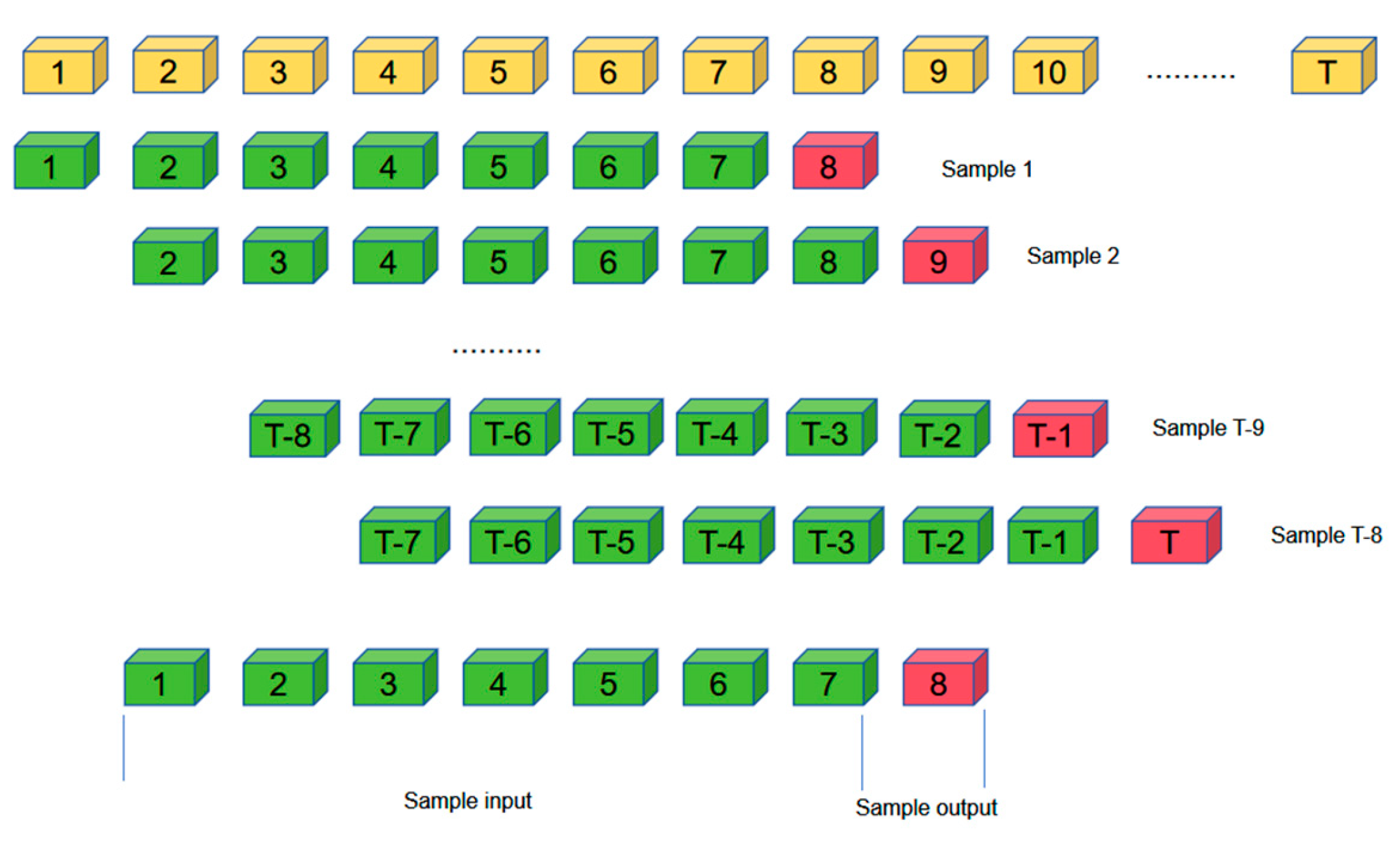
3.2.3. Sample Making

In this study, a sliding window approach is employed to construct sample data for short-term forecasting of the non-stationary rainfall series. Specifically, each sample consists of rainfall data from seven consecutive days as input, with the rainfall value on the eighth day as the prediction target, as illustrated in Figure 9. In the figure, green markers indicate the input data points, while red markers denote the prediction targets. A total of 1820 training samples are generated. Among them, 80% are used for training and the remaining 20% are reserved for testing. To optimize the model’s hyperparameters, cross-validation is conducted on the training set, where 20% of the training data is used as a validation subset in each fold. The final model is then evaluated independently on the test set.

3.2.4. Data Normalization Processing

To improve the training efficiency and prediction stability of the model, the original rainfall time series data were standardized prior to modeling. Due to the inconsistency in scale among different feature dimensions, directly feeding the raw data into the model may result in gradient imbalance or training non-convergence. Therefore, the z-score normalization method was adopted to normalize both the input features and the target outputs. The z-score normalization is calculated using the following formula:

$$x’={\displaystyle \frac{x-\mu }{\sigma }}$$

(20)

where $x$ represents the original data, $\mu$ is the mean of the training samples, $\sigma$ is the standard deviation of the training samples, and $x^{\prime }$ is the normalized data. This method transforms the data into a standard normal distribution with a mean of 0 and a standard deviation of 1, which facilitates faster convergence during the training phase and enhances the predictive performance of neural network models.

In practice, the input features and target outputs of the training set are standardized using the mean and standard deviation computed from the training data. For the test set, the same normalization parameters derived from the training set are applied to ensure consistency in data distribution, thereby improving the model’s generalization capability. During the prediction phase, in order to convert the model output back to the original rainfall scale, an inverse normalization process is applied. The corresponding inverse transformation is given by the following:

$$x=x^{\prime }\cdot \sigma +\mu$$

(21)

Here, $x^{\prime }$ denotes the predicted value from the model, and $x$ represents the actual prediction result after inverse normalization. This post-processing step enables the direct application of the forecasted results in real-world engineering scenarios.

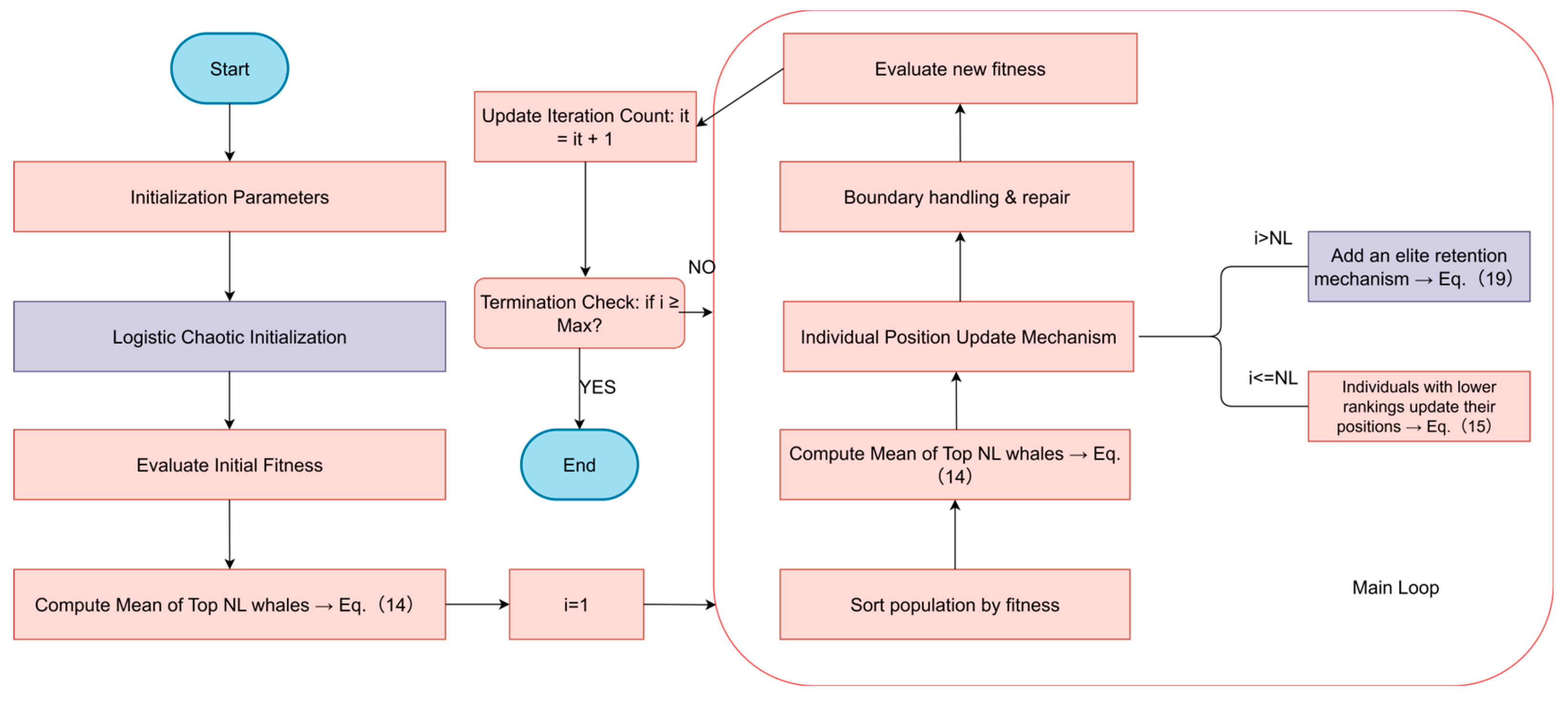
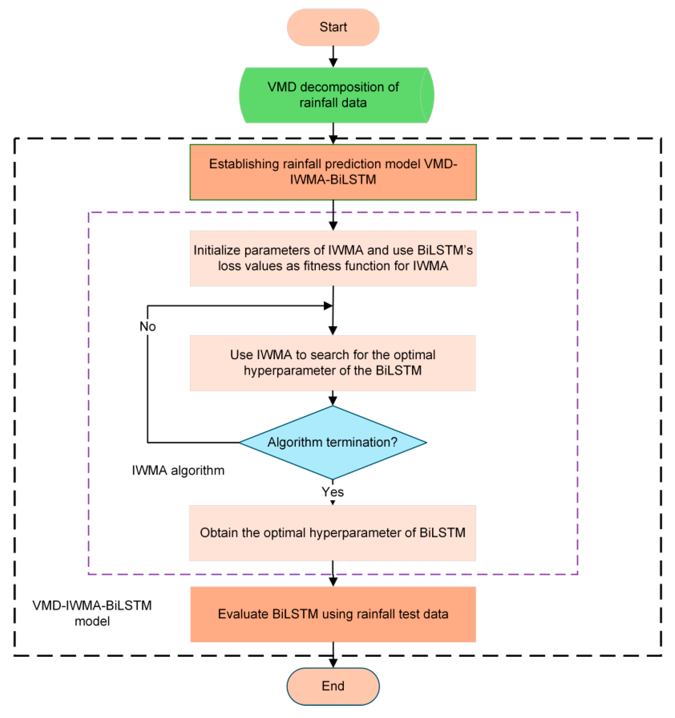
3.2.5. VMD-IWMA-BiLSTM Flowchart

When employing the BiLSTM model for rainfall prediction, the following three hyperparameters have the most significant impact on its predictive performance (1) the number of units in each BiLSTM layer (unit); (2) the learning rate for parameter updates during training (learning_rate); and (3) the maximum number of training epochs (max_epochs).

In this study, the improved IWMA is employed to optimize the three aforementioned hyperparameters. Prior to the optimization process, it is necessary to define the upper and lower bounds of the search space for each hyperparameter. The specific value ranges are presented in

Table 8. Range of values for the hyperparameter.

Hyperparameter Name	Description	Lower Bounds	Upper Bounds
unit	The number of units in the BiLSTM layer	50	300
learning_rate	Parameter update step during model training	0.001	0.01
max_epochs	Maximum number of cycles for model training	50	300

.

Subsequently, the IWMA is initialized with a maximum number of iterations set to 200, dimensionality d is 3, and population size n is 30. The BiLSTM model’s loss function—Root Mean Square Error (RMSE)—is employed as the fitness function in the optimization process. The solver for BiLSTM training is configured as AdaGrad. Finally, the IWMA algorithm is utilized to search for the optimal set of hyperparameters for the BiLSTM model. The overall flowchart of the VMD-IWMA-BiLSTM framework is illustrated in Figure 10.

3.2.6. Evaluation Metrics

This section employs four metrics to evaluate model performance: Mean Absolute Error (MAE), Root Mean Square Error (RMSE), Mean Absolute Percentage Error (MAPE), and Pearson Temporal Correlation Coefficient (PCC). Their calculation formulas are as follows:

$$MAE={\displaystyle \frac{1}{n}}{\displaystyle \sum _{i=1}^n\left|y_i-{\widehat{y}}_i\right|}$$

(22)

$$RMSE=\sqrt{{\displaystyle \frac{1}{n}}{\displaystyle \sum _{i=1}^n{\left(y_i-{\widehat{y}}_i\right)}^2}}$$

(23)

$$MAPE={\displaystyle \frac{1}{n}}{\displaystyle \sum _{i=1}^n\left(\frac{y_i-{\widehat{y}}_i}{y_i}\right)}\times 100\%$$

(24)

$${\rho }_T={\displaystyle \frac{\sum _{t=1}^n(y_t-\overline{y}\left)\right({\widehat{y}}_t-\overline{\widehat{y}})}{\sqrt{\sum (y_t-\overline{y}{)}^2}\sqrt{\sum ({\widehat{y}}_t-\overline{\widehat{y}}{)}^2}}}$$

(25)

where n is the number of test samples, is the actual measured value of the sample data, is the predicted value of the sample data, and is the average measured value of the sample data.

3.2.7. Comparison of BiLSTM Optimized by Various Algorithms

In this section, in addition to IWMA, twelve other optimization algorithms were employed to optimize the proposed BiLSTM-based rainfall prediction model, and their optimization performances were compared. These comparison algorithms include three conventional optimization methods—Grid Search, Random Search, and Bayesian Optimization—as well as eight widely used swarm intelligence algorithms, namely HHO, SCA, GWO, EHO, BOA, WOA, PSO, and DE, along with the original WMA algorithm. To minimize the impact of randomness on the experimental results, each set of comparative experiments was independently repeated 30 times.

The experimental dataset was obtained from the Xinzheng National Meteorological Observatory. The results are presented in

Table 9. Comparison of various models.

Optimization Algorithm	Optimal Solution from the Optimization Algorithm			Evaluation Indicators
	Unit	lr	mp	MAE	RMSE	MAPE	PCC
Grid Search	300	0.0080	50	1.5159	3.4205	34.57%	0.8823
Random Search	225	0.0031	298	1.1283	2.4464	28.59%	0.8932
Bayesian	235	0.0037	287	1.2386	2.6226	25.82%	0.8964
HHO	50	0.0010	50	0.5596	1.2178	9.95%	0.9786
SCA	280	0.0085	50	0.3889	0.8383	6.23%	0.9821
GWO	50	0.0068	172	0.4050	0.8899	6.82%	0.9875
EHO	53	0.0011	64	0.4770	1.0798	7.99%	0.9863
BOA	75	0.0073	286	0.4356	0.9960	7.56%	0.9833
WOA	76	0.0054	114	0.3708	0.7956	6.14%	0.9842
PSO	50	0.0064	177	0.3948	0.8560	6.90%	0.9882
DE	71	0.0040	300	0.3785	0.8380	6.81%	0.9898
WMA	300	0.0010	300	0.3427	0.7109	5.47%	0.9932
IWMA	288	0.0010	258	0.2251	0.3896	3.76%	0.9962

, where the best-performing values are highlighted in bold. The parameters unit, lr, and mp represent the optimal hyperparameters obtained by each algorithm, corresponding to the unit number (number of units in the BiLSTM layer), learning rate, and maximum number of training epochs, respectively, as described in Table 8.

Based on the results in Table 9, it is evident that traditional optimization methods such as grid search, random search, and Bayesian optimization perform significantly worse than swarm intelligence algorithms. Among the ten swarm intelligence algorithms tested, the proposed Improved Whale Migration Algorithm (IWMA) achieved the best performance.

Moreover, the experimental results indicate that different optimization algorithms, when applied to tune the hyperparameters of the same BiLSTM prediction model, can significantly improve its performance to varying degrees. This finding suggests that in deep learning applications, the effectiveness of the optimization strategy plays a decisive role in determining the model’s final performance—sometimes even more critical than the choice of the model architecture itself. Therefore, the rational design and application of efficient optimization algorithms are of great importance for enhancing prediction accuracy.

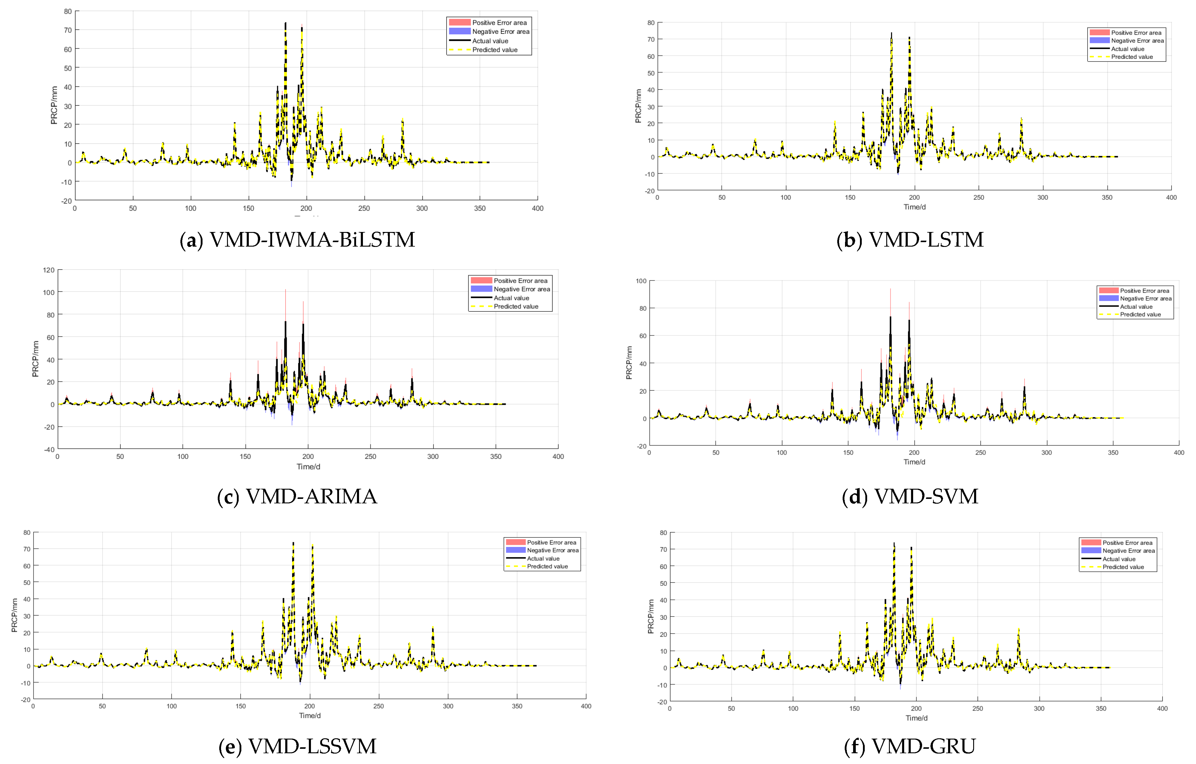
3.2.8. Comparison with Other Models

In the previous section, we analyzed the performance of the BiLSTM model under different optimization algorithms and found that the model optimized by IWMA achieved the best results. To further validate the effectiveness and advantages of this model, this section compares it with five commonly used machine learning and deep learning models, including Support Vector Machine (SVM), Least Squares Support Vector Machine (LSSVM), Gated Recurrent Unit (GRU), and Long Short-Term Memory network (LSTM). In addition, the ARIMA statistical model is introduced as a baseline to comprehensively evaluate the overall performance of the proposed VMD-IWMA-BiLSTM framework in rainfall prediction tasks.

To ensure fairness, all models were optimized using the IWMA algorithm. Each experiment was independently repeated 30 times, and the average values of the evaluation metrics across the 30 runs are presented in

Table 10. Comparative analysis of diverse models.

Detection Station	Model	MAE	RMSE	MAPE	PCC	Rank
Aver (30 Times)
Xinzheng Testing Station, Zhengzhou City	ARIMA	1.4898	3.5715	37.58%	0.8912	6
	SVM	1.1872	2.6111	26.91%	0.9494	5
	LSSVM	0.4239	0.8162	5.19%	0.9744	3
	GRU	0.3368	0.6939	5.09%	0.9869	2
	LSTM	0.3632	0.7553	5.84%	0.9861	4
	BiLSTM	0.2251	0.3896	3.76%	0.9962	1

. The table also reports the performance results of each model, with the best results highlighted in bold. The column “Rank” represents the final ranking of each model based on overall performance. As shown in the results, the BiLSTM model significantly outperforms all other comparison models across all evaluation metrics on the Xinzheng National Meteorological Observatory rainfall dataset, confirming its superior performance in the rainfall forecasting task.

Figure 11 visually compares the predicted and actual rainfall values on the test set for each model. The x-axis represents time, while the y-axis denotes rainfall amount. As clearly illustrated in the plots, the proposed BiLSTM model exhibits the best forecasting performance, with the smallest prediction error, further validating its superiority.

4. Conclusions

To improve the accuracy of rainfall forecasting, this study proposes a hybrid prediction framework that integrates Variational Mode Decomposition (VMD), Improved Whale Migration Algorithm (IWMA) for hyperparameter optimization, and a Bidirectional Long Short-Term Memory (BiLSTM) deep learning model. The framework is empirically validated using daily rainfall data from the Xinzheng National Meteorological Observatory for the period 2020–2024.

The contributions of this paper are as follows:

• To address the nonlinear characteristics of the sample data, this study introduces the Variational Mode Decomposition (VMD) method into the field of rainfall prediction. This approach effectively mitigates the non-stationarity problem of the original sequence, thereby improving modeling accuracy and predictive performance. It provides a novel perspective for modeling complex meteorological time series.
• This paper proposes a VMD-IWMA-BiLSTM framework for rainfall prediction and systematically verifies the superiority of the Improved Whale Migration Algorithm (IWMA) in hyperparameter optimization for deep learning models, as well as its significant enhancement of BiLSTM’s predictive ability.
• In comparative experiments with models such as ARIMA, SVM, LSSVM, RNN, and LSTM, the VMD-IWMA-BiLSTM model demonstrated the best performance in both modeling capability and prediction accuracy, significantly outperforming traditional machine learning and deep learning methods. The study further confirms the effectiveness of IWMA in hyperparameter optimization and the applicability of VMD in handling complex, non-stationary time series.

In conclusion, the VMD-IWMA-BiLSTM framework demonstrates excellent performance in rainfall prediction tasks, providing viable technical pathways and methodological paradigms for improving the accuracy of rainfall time series prediction and addressing the challenges of high randomness.

References

1. Liker, J.K.; Augustyniak, S.; Duncan, G.J. Panel data and models of change: A comparison of first difference and conventional two-wave models. Soc. Sci. Res. 1985, 14, 80–101. [Google Scholar] [CrossRef]
2. West, R.M. Best practice in statistics: The use of log transformation. Ann. Clin. Biochem. 2022, 59, 162–165. [Google Scholar] [CrossRef] [PubMed]
3. De Livera, A.M.; Hyndman, R.J.; Snyder, R.D. Forecasting time series with complex seasonal patterns using exponential smoothing. J. Am. Stat. Assoc. 2011, 106, 1513–1527. [Google Scholar] [CrossRef]
4. Huang, N.E.; Shen, Z.; Long, S.R.; Wu, M.C.; Shih, E.H.; Zheng, Q.; Tung, C.C.; Liu, H.H. The empirical mode decomposition method and the Hilbert spectrum for non-stationary time series analysis. Proc. Roy. Soc. 1998, 454A, 903–995. [Google Scholar] [CrossRef]
5. Wu, Z.; Huang, N.E. Ensemble empirical mode decomposition: A noise-assisted data analysis method. Adv. Adapt. Data Anal. 2009, 1, 1–41. [Google Scholar] [CrossRef]
6. Dragomiretskiy, K.; Zosso, D. Variational mode decomposition. IEEE Trans. Signal Process. 2013, 62, 531–544. [Google Scholar] [CrossRef]
7. Banjade, T.P.; Liu, J.; Li, H.; Ma, J. Enhancing earthquake signal based on variational mode decomposition and SG filter. J. Seismol. 2021, 25, 41–54. [Google Scholar] [CrossRef]
8. Qin, Y.; Zhao, M.; Lin, Q.; Li, X.; Ji, J. Data-driven building energy consumption prediction model based on VMD-SA-DBN. Mathematics 2022, 10, 3058. [Google Scholar] [CrossRef]
9. Masum, M.H.; Islam, R.; Hossen, M.A.; Akhie, A.A. Time series prediction of rainfall and temperature trend using ARIMA model. J. Sci. Res. 2022, 14, 215–227. [Google Scholar] [CrossRef]
10. Karthikeyan, L.; Kumar, D.N. Predictability of nonstationary time series using wavelet and EMD based ARMA models. J. Hydrol. 2013, 502, 103–119. [Google Scholar] [CrossRef]
11. Hussein, E.; Ghaziasgar, M.; Thron, C. Regional rainfall prediction using support vector machine classification of large-scale precipitation maps. In Proceedings of the 2020 IEEE 23rd International Conference on Information Fusion (FUSION), Rustenburg, South Africa, 6–9 July 2020; IEEE: New York, NY, USA; pp. 1–8. [Google Scholar]
12. Ma, M.; Zhao, G.; He, B.; Li, Q.; Dong, H.; Wang, S.; Wang, Z. XGBoost-based method for flash flood risk assessment. J. Hydrol. 2021, 598, 126382. [Google Scholar] [CrossRef]
13. Reddy, P.C.S.; Yadala, S.; Goddumarri, S.N. Development of rainfall forecasting model using machine learning with singular spectrum analysis. IIUM Eng. J. 2022, 23, 172–186. [Google Scholar] [CrossRef]
14. Ma, Z.; Zhang, H.; Liu, J. MM-RNN: A multimodal RNN for precipitation nowcasting. IEEE Trans. Geosci. Remote Sens. 2023, 61, 4101914. [Google Scholar] [CrossRef]
15. Poornima, S.; Pushpalatha, M. Prediction of rainfall using intensified LSTM based recurrent neural network with weighted linear units. Atmosphere 2019, 10, 668. [Google Scholar] [CrossRef]
16. Salehin, I.; Talha, I.M.; Hasan, M.M.; Dip, S.T.; Saifuzzaman, M.; Moon, N.N. An artificial intelligence based rainfall prediction using LSTM and neural network. In Proceedings of the 2020 IEEE International Women in Engineering (WIE) Conference on Electrical and Computer Engineering (WIECON-ECE), Bhubaneswar, India, 26–27 December 2020; IEEE: New York, NY, USA; pp. 5–8. [Google Scholar]
17. Xie, C.; Huang, C.; Zhang, D.; He, W. BiLSTM-I: A deep learning-based long interval gap-filling method for meteorological observation data. Int. J. Environ. Res. Public Health 2021, 18, 10321. [Google Scholar] [CrossRef]
18. Siami-Namini, S.; Tavakoli, N.; Namin, A.S. The performance of LSTM and BiLSTM in forecasting time series. In Proceedings of the 2019 IEEE International Conference on Big Data (Big Data), Los Angeles, CA, USA, 9–12 December 2019; IEEE: New York, NY, USA; pp. 3285–3292. [Google Scholar]
19. Latifoğlu, L. A novel combined model for prediction of daily precipitation data using instantaneous frequency feature and bidirectional long short time memory networks. Environ. Sci. Pollut. Res. 2022, 29, 42899–42912. [Google Scholar] [CrossRef]
20. Khalid, R.; Javaid, N. A survey on hyperparameters optimization algorithms of forecasting models in smart grid. Sustain. Cities Soc. 2020, 61, 102275. [Google Scholar] [CrossRef]
21. Bergstra, J.; Yamins, D.; Cox, D. Making a science of model search: Hyperparameter optimization in hundreds of dimensions for vision architectures. In Proceedings of the International Conference on Machine Learning, PMLR, Atlanta, GA, USA, 17–19 June 2013; pp. 115–123. [Google Scholar]
22. Probst, P.; Boulesteix, A.L.; Bischl, B. Tunability: Importance of hyperparameters of machine learning algorithms. J. Mach. Learn. Res. 2019, 20, 1934–1965. [Google Scholar]
23. El-Kenawy, E.S.M.; Abdelhamid, A.A.; Alrowais, F.; Abotaleb, M.; Ibrahim, A.; Khafaga, D.S. Al-Biruni Based Optimization of Rainfall Forecasting in Ethiopia. Comput. Syst. Sci. Eng. 2023, 46, 2885–2899. [Google Scholar] [CrossRef]
24. Zoremsanga, C.; Hussain, J. Particle swarm optimized deep learning models for rainfall prediction: A case study in Aizawl, Mizoram. IEEE Access 2024, 12, 57172–57184. [Google Scholar] [CrossRef]
25. Amini, A.; Dolatshahi, M.; Kerachian, R. Effects of automatic hyperparameter tuning on the performance of multi-Variate deep learning-based rainfall nowcasting. Water Resour. Res. 2023, 59, e2022WR032789. [Google Scholar] [CrossRef]
26. Shawki, N.; Nunez, R.R.; Obeid, I.; Picone, J. On automating hyperparameter optimization for deep learning applications. In Proceedings of the 2021 IEEE Signal Processing in Medicine and Biology Symposium (SPMB), Philadelphia, PA, USA, 4 December 2021; IEEE: New York, NY, USA; pp. 1–7. [Google Scholar]
27. Belete, D.M.; Huchaiah, M.D. Grid search in hyperparameter optimization of machine learning models for prediction of HIV/AIDS test results. Int. J. Comput. Appl. 2022, 44, 875–886. [Google Scholar] [CrossRef]
28. Alibrahim, H.; Ludwig, S.A. Hyperparameter optimization: Comparing genetic algorithm against grid search and bayesian optimization. In Proceedings of the 2021 IEEE Congress on Evolutionary Computation (CEC), Online, 28 June–1 July 2021; IEEE: New York, NY, USA; pp. 1551–1559. [Google Scholar]
29. Du, L.; Gao, R.; Suganthan, P.N.; Wang, D.Z. Bayesian optimization based dynamic ensemble for time series forecasting. Inf. Sci. 2022, 591, 155–175. [Google Scholar] [CrossRef]
30. Wang, J.; Yang, Z. Ultra-short-term wind speed forecasting using an optimized artificial intelligence algorithm. Renew. Energy 2021, 171, 1418–1435. [Google Scholar] [CrossRef]
31. Xu, M.; Cao, L.; Lu, D.; Hu, Z.; Yue, Y. Application of swarm intelligence optimization algorithms in image processing: A comprehensive review of analysis, synthesis, and optimization. Biomimetics 2023, 8, 235. [Google Scholar] [CrossRef]
32. Venkatesh, C.; Prasad, B.V.V.S.; Khan, M.; Babu, J.C.; Dasu, M.V. An automatic diagnostic model for the detection and classification of cardiovascular diseases based on swarm intelligence technique. Heliyon 2024, 10, e25574. [Google Scholar] [CrossRef] [PubMed]
33. Gaspar, A.; Oliva, D.; Cuevas, E.; Zaldívar, D.; Pérez, M.; Pajares, G. Hyperparameter optimization in a convolutional neural network using metaheuristic algorithms. In Metaheuristics in Machine Learning: Theory and Applications; Springer International Publishing: Cham, Switzerland, 2021; pp. 37–59. [Google Scholar]
34. Heidari, A.A.; Mirjalili, S.; Faris, H.; Aljarah, I.; Mafarja, M.; Chen, H. Harris hawks optimization: Algorithm and applications. Future Gener. Comput. Syst. 2019, 97, 849–872. [Google Scholar] [CrossRef]
35. Mirjalili, S. SCA: A sine cosine algorithm for solving optimization problems. Knowl.-Based Syst. 2016, 96, 120–133. [Google Scholar] [CrossRef]
36. Mirjalili, S.; Mirjalili, S.M.; Lewis, A. Grey wolf optimizer. Adv. Eng. Softw. 2014, 69, 46–61. [Google Scholar] [CrossRef]
37. Al-Betar, M.A.; Awadallah, M.A.; Braik, M.S.; Makhadmeh, S.; Doush, I.A. Elk herd optimizer: A novel nature-inspired metaheuristic algorithm. Artif. Intell. Rev. 2024, 57, 48. [Google Scholar] [CrossRef]
38. Arora, S.; Singh, S. Butterfly optimization algorithm: A novel approach for global optimization. Soft Comput. 2019, 23, 715–734. [Google Scholar] [CrossRef]
39. Seyedali, M.; Lewis, A. The Whale Optimization Algorithm. Adv. Eng. Softw. 2015, 95, 51–67. [Google Scholar]
40. Marini, F.; Walczak, B. Particle swarm optimization (PSO). A tutorial. Chemom. Intell. Lab. Syst. 2015, 149, 153–165. [Google Scholar] [CrossRef]
41. Storn, R.; Price, K. Differential evolution–a simple and efficient heuristic for global optimization over continuous spaces. J. Glob. Optim. 1997, 11, 341–359. [Google Scholar] [CrossRef]
42. Joyce, T.; Herrmann, J.M. A review of no free lunch theorems, and their implications for metaheuristic optimisation. In Nature-Inspired Algorithms and Applied Optimization; Springer: Berlin/Heidelberg, Germany, 2017; pp. 27–51. [Google Scholar]
43. Adam, S.P.; Alexandropoulos, S.A.N.; Pardalos, P.M.; Vrahatis, M.N. No free lunch theorem: A review. In Approximation and Optimization: Algorithms, Complexity and Applications; Springer: Berlin/Heidelberg, Germany, 2019; pp. 57–82. [Google Scholar]
44. Ghasemi, M.; Deriche, M.; Trojovský, P.; Mansor, Z.; Zare, M.; Trojovská, E.; Abualigah, L.; Ezugwu, A.E.; Mohammadi, S.K. An efficient bio-inspired algorithm based on humpback whale migration for constrained engineering optimization. Results Eng. 2025, 25, 104215. [Google Scholar] [CrossRef]
45. Varol Altay, E.; Alatas, B. Bird swarm algorithms with chaotic mapping. Artif. Intell. Rev. 2020, 53, 1373–1414. [Google Scholar] [CrossRef]
46. Wang, F.; Zhou, L.; Ren, H.; Liu, X. Search improvement process-chaotic optimization-particle swarm optimization-elite retention strategy and improved combined cooling-heating-power strategy based two-time scale multi-objective optimization model for stand-alone microgrid operation. Energies 2017, 10, 1936. [Google Scholar] [CrossRef]
47. Wu, G.; Mallipeddi, R.; Suganthan, P.N. Problem Definitions and Evaluation Criteria for the CEC 2017 Competition on Constrained Real-Parameter Optimization; National University of Defense Technology: Changsha, China; Kyungpook National University: Daegu, Republic of Korea; Nanyang Technological University: Singapore, 2017. [Google Scholar]
48. Yang, Y.; Li, S.; Liu, H.; Guo, J. Carbon Dioxide Emission Forecasting Using BiLSTM Network Based on Variational Mode Decomposition and Improved Black-Winged Kite Algorithm. Mathematics 2025, 13, 1895. [Google Scholar] [CrossRef]
Figure 1. LSTM state gating structure.
Mathematics 13 02483 g001
Figure 2. BiLSTM model structure diagram.
Mathematics 13 02483 g002
Figure 3. Workflow of the Whale Migration Algorithm inspired by humpback whale behavior.
Mathematics 13 02483 g003
Figure 4. Flowchart of IWMA.
Mathematics 13 02483 g004
Figure 5. The Friedman rankings of different algorithms on 29 benchmark functions.
Mathematics 13 02483 g005
Figure 6. Fitness curve comparison across algorithms during iterative processes.
Mathematics 13 02483 g006
Figure 7. Daily rainfall data from 2020 to 2024.
Mathematics 13 02483 g007
Figure 8. Results of VMD decomposition.
Mathematics 13 02483 g008
Figure 9. Sample making map.
Mathematics 13 02483 g009
Figure 10. VMD-IWMA-BiLSTM framework.
Mathematics 13 02483 g010
Figure 11. Error curves of different models.
Mathematics 13 02483 g011