Bidirectional Conservative–Dissipative Transitions in a Five-Dimensional Fractional Chaotic System

Abstract

This study investigates a modified five-dimensional chaotic system by incorporating structural term adjustments and Caputo fractional-order differential operators. The modified system exhibits significantly enriched dynamic behaviors, including offset boosting, phase trajectory rotation, phase trajectory reversal, and contraction phenomena. Additionally, the system exhibits bidirectional transitions—conservative-to-dissipative transitions governed by initial conditions and dissipative-to-conservative transitions controlled by fractional order variations—along with a unique chaotic-to-quasiperiodic transition observed exclusively at low fractional orders. To validate the system’s physical realizability, a signal processing platform based on Digital Signal Processing (DSP) is implemented. Experimental measurements closely align with numerical simulations, confirming the system’s feasibility for practical applications.

1. Introduction

Chaos, as a ubiquitous phenomenon in natural and engineered systems, has remained a focal point of scientific research due to its intrinsic complexity and broad applicability. Its unique value manifests across diverse domains: from deciphering intricate dynamics in neural networks [1,2] and unraveling nonlinear behaviors in biological systems [3,4] to addressing security demands in image encryption and secure communication [5,6]. Characterized by aperiodicity, extreme sensitivity to initial conditions, and rich attractor topologies, chaotic behavior fundamentally encapsulates the essence of complex systems. Concurrently, fractional-order calculus has gained significant traction in nonlinear dynamics research, offering enhanced precision in modeling real-world systems with memory-dependent and non-local properties. This mathematical framework has permeated interdisciplinary fields, including material physics [7], electromagnetic wave propagation [8,9], ecological systems [10,11], robotic locomotion [12], and photonics [13], as well as all aspects of life [14,15,16]. Within this landscape, fractional-order chaotic systems—emerging from the synergy of chaos theory and fractional calculus—represent a transformative frontier. These systems demonstrate unparalleled dynamical characteristics, establishing fractional-order chaos as a pivotal methodology for advancing nonlinear science and its engineering applications.

Significant advancements have been made in the study of conservative chaotic systems, revealing the fundamental characteristics of chaotic phenomena. In 2014, Vaidyanathan et al. proposed modified three-dimensional conservative chaotic systems based on the Nosé–Hoover framework over two consecutive years, conducting in-depth analyses of their conservative dynamics [17,18]. By 2017, Cang et al. introduced two four-dimensional autonomous conservative chaotic systems [19], rigorously verifying their conservative nature using the trace of the Jacobian matrix, perpetual point theory [20,21], and Hamiltonian energy theory.

In 2018, Wu et al. developed a five-dimensional conservative chaotic system and identified hyperchaotic behavior within conservative systems for the first time [22]. Concurrently, Cang et al. discovered that certain non-conservative chaotic systems can also exhibit conservative chaotic flows [23]. That same year, Singh et al. constructed five specialized conservative chaotic systems and observed coexistence phenomena between chaotic flows, as well as between chaotic and quasi-periodic flows [24]. Further expanding the field, Gu et al. (2020) designed a four-dimensional conservative chaotic system incorporating memristors, which demonstrated hidden extreme multistability and initial-offset boosting behavior [25]. Most recently, Zhang et al. (2022) proposed a novel methodology for constructing cyclically symmetric conservative chaotic systems applicable to three-dimensional and higher-dimensional systems, validating both the conservative and chaotic properties of these systems to confirm the approach’s feasibility [26].

Fractional-order dynamical systems are typically derived from their integer-order counterparts by replacing standard differential operators with fractional-order ones. This approach has been successfully applied to classical systems such as the fractional-order Lorenz [27], Chen [28], Chua [29], Lü [30], and Jerk systems [31]. Remarkably, the resulting fractional-order systems not only retain chaotic and periodic behaviors but also exhibit unique dynamical phenomena, reigniting global scholarly interest in fractional calculus and its applications. Notable contributions include Donato et al.’s investigation of a fractional-order chaotic system without equilibrium points, which demonstrated hyperchaos for orders below 3.84, with particular emphasis on the dynamics at q = 0.96 [32]. Zhang et al. developed a four-dimensional fractional-order hyperchaotic system using feedback control, reporting the first observation of initial value-dependent antimonotonicity [33]. While these studies focused on dissipative chaotic systems, fractional-order conservative chaotic systems represent a distinct class with more complex and unpredictable dynamics compared to their dissipative counterparts. These systems hold significant theoretical importance and practical potential. Recent advances include the following: Leng et al. (2021): a four-dimensional fractional-order system exhibiting both dissipative and conservative properties, solved via the Adomian Decomposition Method (ADM), revealed order-dependent transitions (q-increasing) from dissipative to conservative dynamics alongside transient behaviors [34]; Tian et al. (2021): a novel five-dimensional conservative hyperchaotic system displayed rich dynamics, including offset boosting, multistability, and distinctive transient phenomena through parameter and order variations [35]. This present study advances the field by modifying a five-dimensional fractional-order chaotic system with the following distinctive features: parametric sensitivity: Exhibits rich dynamical behaviors—including offset boosting, phase-space rotation, phase-space contraction, and large-scale hyperchaos regions. Conservative-to-dissipative transitions: This system undergoes a conservative-to-dissipative transition as the initial values vary. Dissipative-to-conservative transitions: This system transitions from dissipative to conservative as the fractional order q varies. Temporal phenomena: Demonstrates phase trajectory reversal during time evolution along with a unique chaotic-to-quasiperiodic transition observed exclusively at low fractional orders.

Paper organization: Section 2: Introduction of a 5D fractional-order chaotic system, with analysis of its phase trajectories, offset-boosting, rotation, contraction, and reversal behaviors. Section 3: Exploration of nonlinear dynamics, including hyperchaotic regions, conservative-to-dissipative transitions, and fractional-order-controlled dynamics. Section 4: DSP-based hardware implementation and verification. Section 5: Conclusion of the study.

2. Fundamental Dynamics and Phenomena

2.1. Five-Dimensional System Construction and Analysis

Currently, chaotic systems are mainly applied in chaotic image encryption. Among them, five-dimensional chaotic systems can be more effectively integrated with image encryption algorithms. In Figure 1, we illustrate a general approach for fusing a five-dimensional system with an encryption algorithm for reference.

Therefore, building upon the framework established in prior work [36], we modified its first, fourth, and fifth terms to construct the chaotic system, as seen in Equation (1):

$$\left\{\begin{array}{l}\dot{x}=-ay+eux\hfill \\ \dot{y}=ax+bz\hfill \\ \dot{z}=-by+cw\hfill \\ \dot{w}=-cz+du\hfill \\ \dot{u}=1-dw-e{x}^2\hfill \end{array}\right.$$

(1)

where x, y, z, w, and u denote the state variables, and a, b, c, d, and e represent the parameters.

We broke the characteristic of conservative chaotic systems where the dissipation degree is always equal to 0. The calculation formula for the dissipation degree is shown in Equation (2):

$$\nabla V={\displaystyle \frac{\mathsf{\partial }\dot{x}}{\mathsf{\partial }x}}+{\displaystyle \frac{\mathsf{\partial }\dot{y}}{\mathsf{\partial }y}}+{\displaystyle \frac{\mathsf{\partial }\dot{z}}{\mathsf{\partial }z}}+{\displaystyle \frac{\mathsf{\partial }\dot{w}}{\mathsf{\partial }w}}+{\displaystyle \frac{\mathsf{\partial }\dot{\mathrm{u}}}{\mathsf{\partial }u}}=eu$$

(2)

From the calculation results, the dissipation degree of system (1) is not always equal to 0 but changes with parameter e and variable u. This phenomenon endows the system with the ability to switch between conservative and dissipative states [37]. Additionally, an analysis of equilibrium points reveals that the system lacks any finite real equilibria.

According to References [38,39], fractional-order chaotic systems exhibit richer and more complex dynamical behaviors. Therefore, in system (1), through the incorporation of the Caputo fractional derivative operator [40], we derive the fractional-order representation shown in Equation (3):

$$\left\{\begin{array}{l}{}^{c}D_{t_0}^{q}x=-ay+eux\hfill \\ {}^{c}D_{t_0}^{q}y=ax+bz\hfill \\ {}^{c}D_{t_0}^{q}z=-by+cw\hfill \\ {}^{c}D_{t_0}^{q}w=-cz+du\hfill \\ {}^{c}D_{t_0}^{q}u=1-dw-e{x}^2\hfill \end{array}\right.$$

(3)

where ${}^{c}D_{t_0}^q$ signifies the fractional differential operator of order q ∈ (0,1], with t₀ indicating initial time. Current numerical methods for solving fractional-order systems include the homotopy perturbation algorithm, the Adomian Decomposition Method (ADM), and frequency-domain algorithms based on the Laplace transform. Notably, ADM demonstrates unparalleled advantages over other approaches, achieving exceptional computational efficiency and high-precision approximate solutions in computer implementations. This method has shown significant progress in solving fractional-order chaotic systems [41,42,43,44,45,46]. As the number of iterations of the fractional-order solution increases, the accuracy improves, but the corresponding simulation time also rises. However, an excessive iteration count may lead to diminishing returns or even degraded performance; therefore, the iteration number of the ADM algorithm in this paper is set to 5. According to the ADM method, the approximate solution of system (3) can be expressed as Equation (4):

$${\tilde{x}}_j=c_j^0+c_j^1{\displaystyle \frac{{(t-t_0)}^q}{\mathrm{\Gamma }(q+1)}}+c_j^2{\displaystyle \frac{{(t-t_0)}^{2q}}{\mathrm{\Gamma }(2q+1)}}+c_j^3{\displaystyle \frac{{(t-t_0)}^{3q}}{\mathrm{\Gamma }(3q+1)}}+c_j^4{\displaystyle \frac{{(t-t_0)}^{4q}}{\mathrm{\Gamma }(4q+1)}}+c_j^5{\displaystyle \frac{{(t-t_0)}^{5q}}{\mathrm{\Gamma }(5q+1)}}$$

(4)

Additionally, in computer simulations, the time interval [t₀, t] should be as small as possible. It can be divided into several small subintervals: {[t₀, t₁], [t₁, t₂],…, [t_l−1, t_l]}. These l subintervals have the same step size, denoted as h.

Equation (4) can also be written as:

$$\left[\begin{array}{l}\tilde{x}\hfill \\ \tilde{y}\hfill \\ \tilde{z}\hfill \\ \tilde{w}\hfill \\ \tilde{u}\hfill \end{array}\right]=\left|\begin{array}{llllll}{c}_0^1\hfill & c_1^1\hfill & c_2^1\hfill & c_3^1\hfill & c_4^1\hfill & c_5^1\hfill \\ c_0^2\hfill & c_1^2\hfill & c_2^2\hfill & c_3^2\hfill & c_4^2\hfill & c_5^2\hfill \\ c_0^3\hfill & c_1^3\hfill & c_2^3\hfill & c_3^3\hfill & c_4^3\hfill & c_5^3\hfill \\ c_0^4\hfill & c_1^4\hfill & c_2^4\hfill & c_3^4\hfill & c_4^4\hfill & c_5^4\hfill \\ c_0^5\hfill & c_1^5\hfill & c_2^5\hfill & c_3^5\hfill & c_4^5\hfill & c_5^5\hfill \end{array}\right|\times \left|\begin{array}{l}\begin{array}{ccc}& 1& \end{array}\hfill \\ {\displaystyle \frac{h^q}{\Gamma (q+1)}}\hfill \\ {\displaystyle \frac{h^{2q}}{\Gamma (2q+1)}}\hfill \\ {\displaystyle \frac{h^{3q}}{\Gamma (3q+1)}}\hfill \\ {\displaystyle \frac{h^{4q}}{\Gamma (4q+1)}}\hfill \\ {\displaystyle \frac{h^{5q}}{\Gamma (5q+1)}}\hfill \end{array}\right|$$

(5)

$$\left\{\begin{array}{l}\begin{array}{l}{c}_0^1=x(t_0)\\ c_0^2=y(t_0)\end{array}\hfill \\ c_0^3=z(t_0)\hfill \\ \begin{array}{l}{c}_0^4=w(t_0)\\ c_0^5=u(t_0)\end{array}\hfill \end{array}\right.$$

(6)

$$\left\{\begin{array}{l}\begin{array}{l}{c}_1^1=-a{c}_0^2+e{c}_0^5{c}_0^1\\ c_1^2=a{c}_0^1+b{c}_0^3\end{array}\hfill \\ c_1^3=-b{c}_0^2+c{c}_0^4\hfill \\ \begin{array}{l}{c}_1^4=-c{c}_0^3+d{c}_0^5\\ c_1^5=1-d{c}_0^4-e{c}_0^1{c}_0^1\end{array}\hfill \end{array}\right.$$

(7)

$$\left\{\begin{array}{l}\begin{array}{l}{c}_2^1=-a{c}_1^2+e(c_1^1{c}_0^5+c_0^1{c}_1^5)\\ c_2^2=a{c}_1^1+b{c}_1^3\end{array}\hfill \\ c_2^3=-b{c}_1^2+c{c}_1^4\hfill \\ \begin{array}{l}{c}_2^4=-c{c}_1^3+d{c}_1^5\\ c_2^5=1-d{c}_1^4-2e{c}_0^1{c}_1^1\end{array}\hfill \end{array}\right.$$

(8)

$$\left\{\begin{array}{l}\begin{array}{l}{c}_3^1=-a{c}_2^2+e\left(c_1^1{c}_1^5+c_2^1{c}_0^5+c_0^1{c}_1^5{\displaystyle \frac{\Gamma (2q+1)}{\Gamma (q+1)\Gamma (q+1)}}\right)\\ c_3^2=a{c}_2^1+b{c}_2^3\end{array}\hfill \\ c_3^3=-b{c}_2^2+c{c}_2^4\hfill \\ \begin{array}{l}{c}_3^4=-c{c}_2^3+d{c}_2^5\\ c_3^5=1-d{c}_2^4-e\left(2c_0^1{c}_2^1+c_1^1{c}_1^1{\displaystyle \frac{\Gamma (2q+1)}{\Gamma (q+1)\Gamma (q+1)}}\right)\end{array}\hfill \end{array}\right.$$

(9)

$$\left\{\begin{array}{l}\begin{array}{l}{c}_4^1=-a{c}_3^2+e\left((c_1^1{c}_2^5+c_2^1{c}_1^5){\displaystyle \frac{\Gamma (3q+1)}{\Gamma (q+1)\Gamma (2q+1)}}+c_0^1{c}_3^5+c_3^1{c}_0^5\right)\\ c_4^2=a{c}_3^1+b{c}_3^3\end{array}\hfill \\ c_4^3=-b{c}_3^2+c{c}_3^4\hfill \\ \begin{array}{l}{c}_4^4=-c{c}_3^3+d{c}_3^5\\ c_4^5=1-d{c}_3^4-e\left(2c_0^1{c}_3^1+2c_2^1{c}_1^1{\displaystyle \frac{\Gamma (3q+1)}{\Gamma (q+1)\Gamma (2q+1)}}\right)\end{array}\hfill \end{array}\right.$$

(10)

$$\left\{\begin{array}{l}\begin{array}{l}{c}_5^1=-a{c}_4^2+e\left((c_1^1{c}_3^5+c_3^1{c}_1^5){\displaystyle \frac{\Gamma (4q+1)}{\Gamma (q+1)\Gamma (3q+1)}}+c_2^1{c}_2^5{\displaystyle \frac{\Gamma (4q+1)}{\Gamma (2q+1)\Gamma (2q+1)}}+c_0^1{c}_4^5+c_4^1{c}_0^5\right)\\ c_5^2=a{c}_4^1+b{c}_4^3\end{array}\hfill \\ c_5^3=-b{c}_4^2+c{c}_4^4\hfill \\ \begin{array}{l}{c}_5^4=-c{c}_4^3+d{c}_4^5\\ c_5^5=1-d{c}_4^4-e\left(2c_0^1{c}_4^1+2c_3^1{c}_1^1{\displaystyle \frac{\Gamma (4q+1)}{\Gamma (q+1)\Gamma (3q+1)}}+c_2^1{c}_2^1{\displaystyle \frac{\Gamma (4q+1)}{\Gamma (2q+1)\Gamma (2q+1)}}\right)\end{array}\hfill \end{array}\right.$$

(11)

To further validate the correctness of this solution method, we conducted verification tests when q = 1 (where the system becomes an integer-order system). Using the ADM method, we plotted phase trajectories and compared them with results obtained through the integer-order solution method—the Runge–Kutta method. The corresponding pseudo-code is given in

Table 1. Runge–Kutta algorithm for system.

Input: x0, h, q, a, b, c, d, e, nsteps:  Output: xs, ys, zs, ws, us

1: xs(1) = x0; ys(1) = y0; zs(1) = z0; us(1) = u0; vs(1) = v0; 2: for i = 1:nsteps-1 3: k1x = h*(-ays(i)+exs(i)vs(i)); 4: k1y = h(axs(i)+bzs(i)); 5: k1z = h*(-bys(i)+cus(i)); 6: k1u = h*(-czs(i)+dvs(i)); 7: k1v = h*(1-dus(i)-exs(i)^2); 8: k2x = h*(-a*(ys(i)+0.5k1y)+e(xs(i)+0.5k1x)(vs(i)+0.5k1v)); 9: k2y = h(a*(xs(i)+0.5k1x)+b(zs(i)+0.5k1z)); 10: k2z = h(-b*(ys(i)+0.5k1y)+c(us(i)+0.5k1u)); 11: k2u = h(-c*(zs(i)+0.5k1z)+d(vs(i)+0.5k1v)); 12: k2v = h(1-d*(us(i)+0.5k1u)-e(xs(i)+0.5k1x)^2); 13: k3x = h(-a*(ys(i)+0.5k2y)+e(xs(i)+0.5k2x)(vs(i)+0.5k2v)); 14: k3y = h(a*(xs(i)+0.5k2x)+b(zs(i)+0.5k2z)); 15: k3z = h(-b*(ys(i)+0.5k2y)+c(us(i)+0.5k2u)); 16: k3u = h(-c*(zs(i)+0.5k2z)+d(vs(i)+0.5k2v)); 17: k3v = h(1-d*(us(i)+0.5k2u)-e(xs(i)+0.5k2x)^2); 18: k4x = h(-a*(ys(i)+k3y)+e*(xs(i)+k3x)(vs(i)+k3v)); 19: k4y = h(a*(xs(i)+k3x)+b*(zs(i)+k3z)); 20: k4z = h*(-b*(ys(i)+k3y)+c*(us(i)+k3u)); 21: k4u = h*(-c*(zs(i)+k3z)+d*(vs(i)+k3v)); 22: k4v = h*(1-d*(us(i)+k3u)-e*(xs(i)+k3x)^2); 23: xs(i+1) = xs(i)+(k1x+2k2x+2k3x+k4x)/6; 24: ys(i+1) = ys(i)+(k1y+2k2y+2k3y+k4y)/6; 25: zs(i+1) = zs(i)+(k1z+2k2z+2k3z+k4z)/6; 26: us(i+1) = us(i)+(k1u+2k2u+2k3u+k4u)/6; 27: vs(i+1) = vs(i)+(k1v+2k2v+2k3v+k4v)/6; 28: end 29: return xs, ys, zs, ws, us

.

A comparison between Figure 2 and Figure 3 reveals that the phase trajectory comparison showed identical results from both methods, confirming the validity of the ADM solution approach used in our analysis.

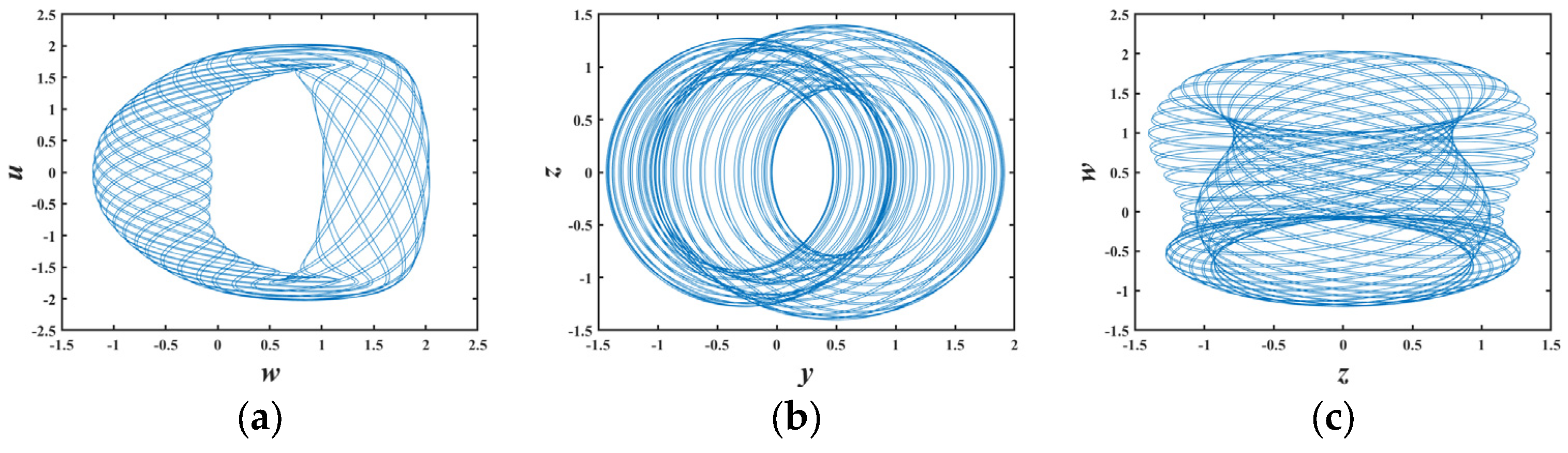
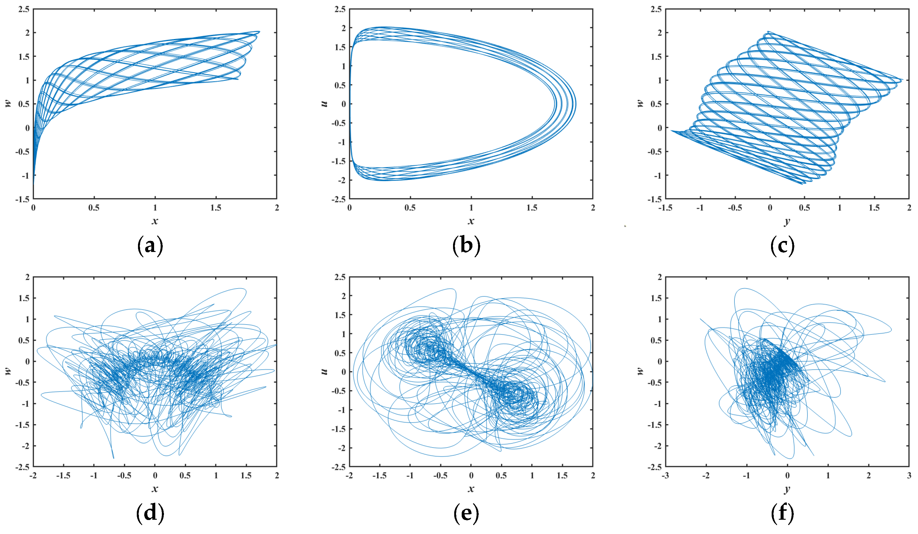
2.2. Phase Trajectory Diagram

To comprehensively demonstrate the system’s dynamic behavior, this section provides the parameters for two distinct system states: quasi-periodic and chaotic.

Quasi-period: a = 0, b = 4, c = 2, d = 1, e = 2, q = 0.98; initial values (1.2, 1.2, 1.2, 1.2, 1.2).

Chaos: a = 7, b = 7, c = 7, d = 7, e = 7, q = 0.98; initial values (1.2, 1.2, 1.2, 1.2, 1.2).

The corresponding phase diagrams (x–w plane, x–u plane, and y–w plane) for these two initial conditions are shown in Figure 4. It is evident that the surfaces in Figure 4a–c are smooth, indicating quasi-periodic motion. In contrast, Figure 4d–f shows irregular patterns, representing chaotic motion.

Meanwhile, the Poincaré cross sections and time series diagrams shown in Figure 5 and Figure 6 can further verify the quasi-periodic and chaotic states of the system.

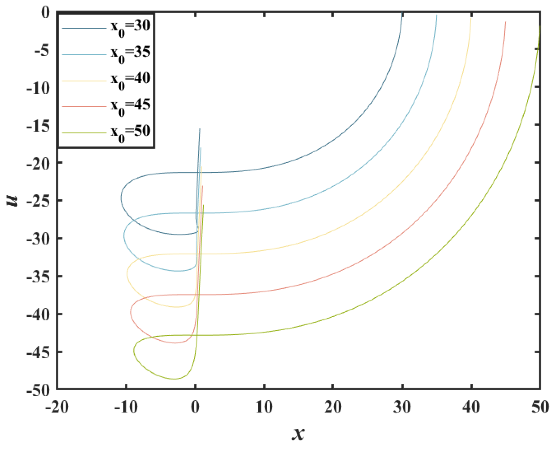
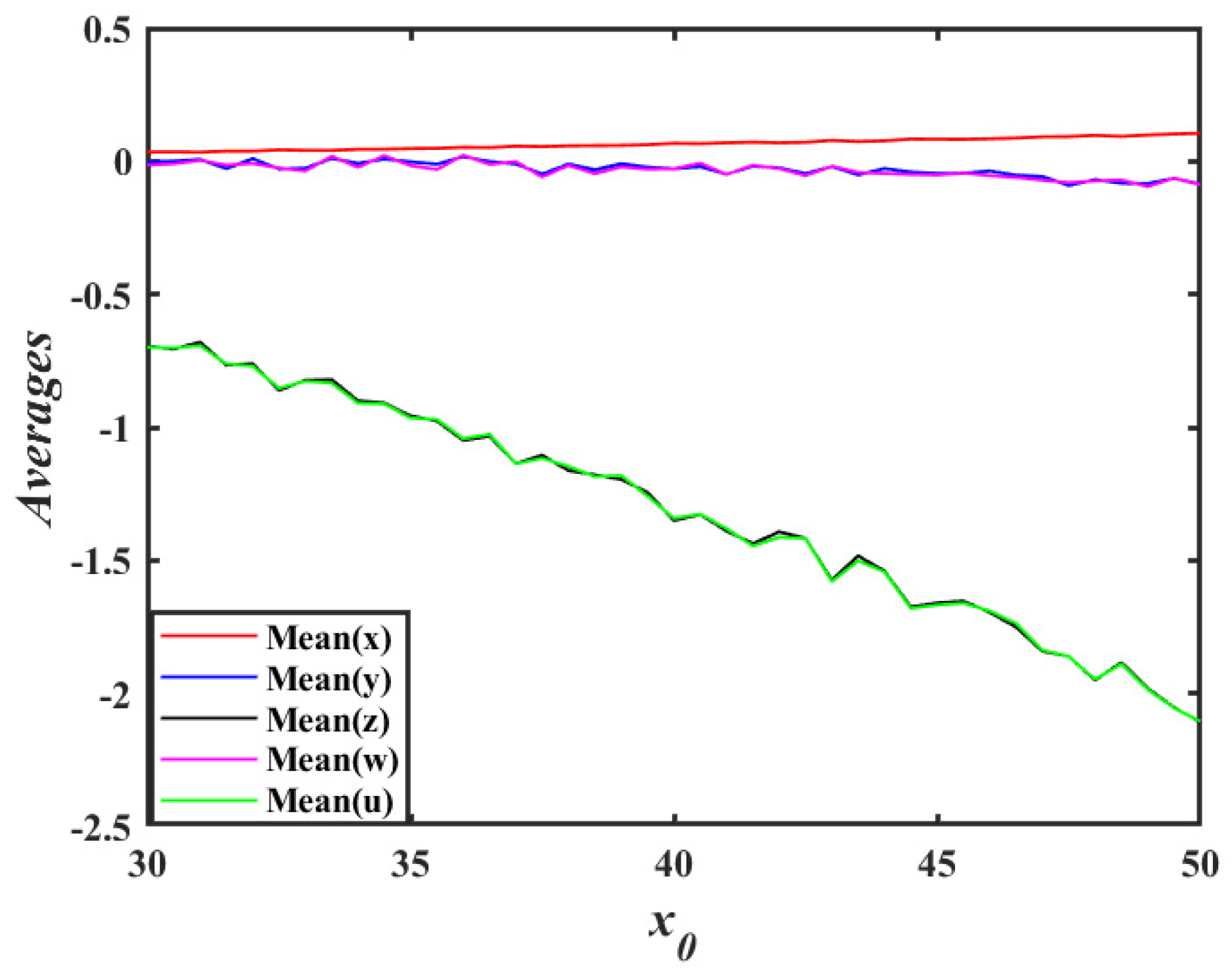
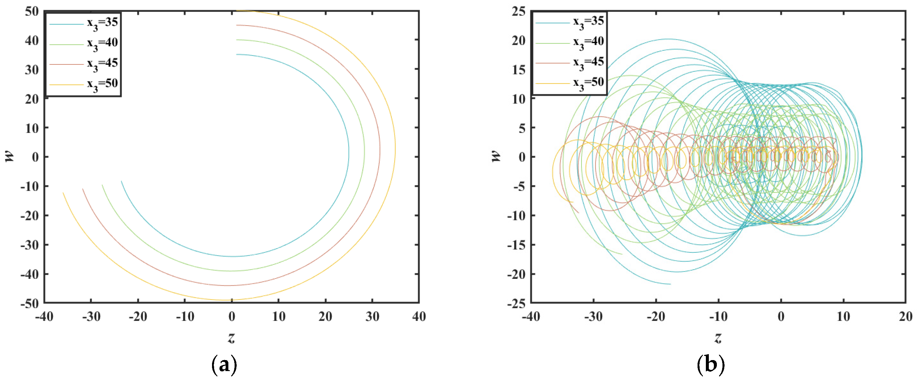
2.3. Offset Boost Behavior

In this subsection, the offset boost behavior in the system will be explained using phase diagrams. When the initial value x₀ is the variable and the parameter configuration is selected as a = 20, b = 1, c = 1, d = 1, e = 1, q = 0.98, y₀ = 1; z₀ = 1; w₀ = 1; u₀ = 1, the x–u phase trajectory diagrams for x₀ = 30, 35, 40, 45, 50 are shown in Figure 7. Examining these figures, numerical simulations show that the system’s phase space trajectories display displacement behavior in both the x and u directions. As x₀ increases, the phase trajectories in Figure 7 show varying degrees of offset in both the x and u directions, overall appearing to shift along the u–axis.

The offset boosting phenomenon can be effectively characterized by examining the mean values of system variables. Figure 8 demonstrates the x₀-dependence of mean values for all state variables. It can be observed that the mean values of x and u show systematic variation with increasing x₀, confirming attractor displacement along these axes. In fact, the phase trajectories of system (3) also show a significant shift along the z–axis.

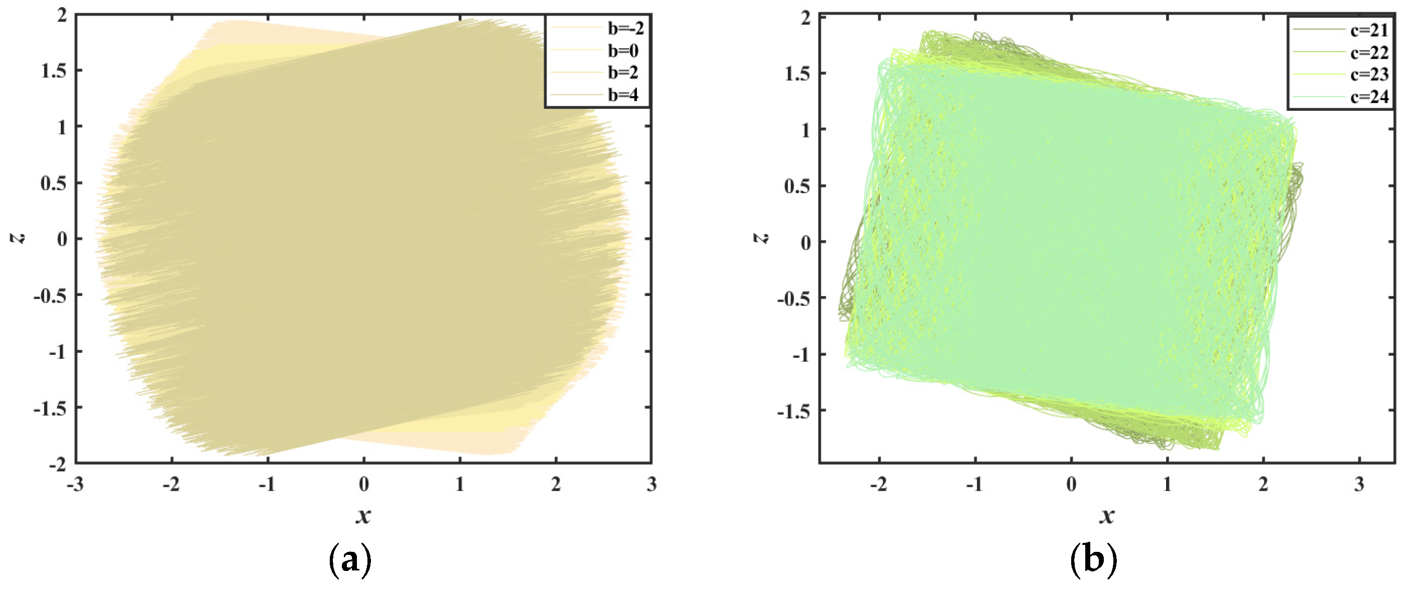
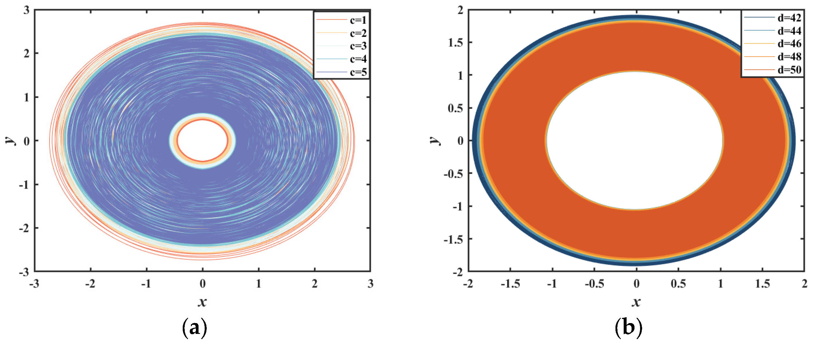
2.4. Rotational Behavior

The motion state of a chaotic system depends directly on its parameters, and selecting appropriate parameters can lead to diverse dynamic behaviors. When examining the role of parameter b in system (3), with a = 20, c = 1, d = 1, e = 1, q = 0.98, and all other initial values set to 1, the experimental results show that as b increases, the system’s phase trajectories rotate around fixed points in the phase space, as shown in the x–z phase diagrams in Figure 9a. For four values of b (−2, 0, 2, 4), the trajectories display increasing rotation with increasing b. Similarly, Figure 9b illustrates the x–z phase diagrams for varying c, with a = 20, b = 1, d = 1, e = 1, q = 0.98, and other initial values fixed at 1. For c values of (21, 22, 23, 24), the phase trajectories also show rotational behavior as c increases.

2.5. Contraction Behavior

In this subsection, the system’s scaling behavior with parameter variations is demonstrated. When c is the control variable and the other parameters are fixed at a = 20, b = 1, d = 1, e = 1, q = 0.98 with all initial values set to 1, the phase trajectories of system (3) contract as c increases. This is illustrated in the x–y phase diagrams in Figure 10a, where five values of c (1, 2, 3, 4, 5) show the trajectories contracting inward with increasing c. Similarly, when d is the control variable and the other parameters are set to a = 20, b = 1, c = 1, e = 1, q = 0.98 with all initial values at 1, the phase trajectories of system (3) also contract as d increases. This behavior is depicted in the x–y phase diagrams in Figure 10b. For five values of d (42, 44, 46, 48, 50), the phase trajectories contract inward as d increases.

2.6. Phase Trajectory Reversal

System (3) displays additional intriguing dynamical phenomena under the parameters set to (a, b, c, d, e, q) = (20, 1, 1, 1, 1, 0.98), starting from initial conditions uniformly set to 1. When x₃ is selected as the control variable, the z–w phase trajectories for x₃ = {35, 40, 45, 50} are plotted in Figure 11. Observations reveal a phase trajectory reversal mechanism: contraction dynamics, where trajectories initialized with larger x₃ values progressively contract into smaller phase-space regions over time, and expansion dynamics, where trajectories starting from smaller x₃ values expand into broader domains during evolution. To clarify this counterintuitive behavior, Figure 12 compares instantaneous phase trajectories at different times: the initial phase (Figure 12a), where phase trajectories are expansive for large x₃ and compact for small x₃, and the late phase (Figure 12b), where an inverted amplitude distribution emerges, with contracted trajectories for initially large and expanded trajectories for initially small.

This self-regulating amplitude inversion indicates a hidden energy redistribution mechanism governed by initial condition sensitivity, challenging conventional stability paradigms in systems.

3. Nonlinear Regime Analysis

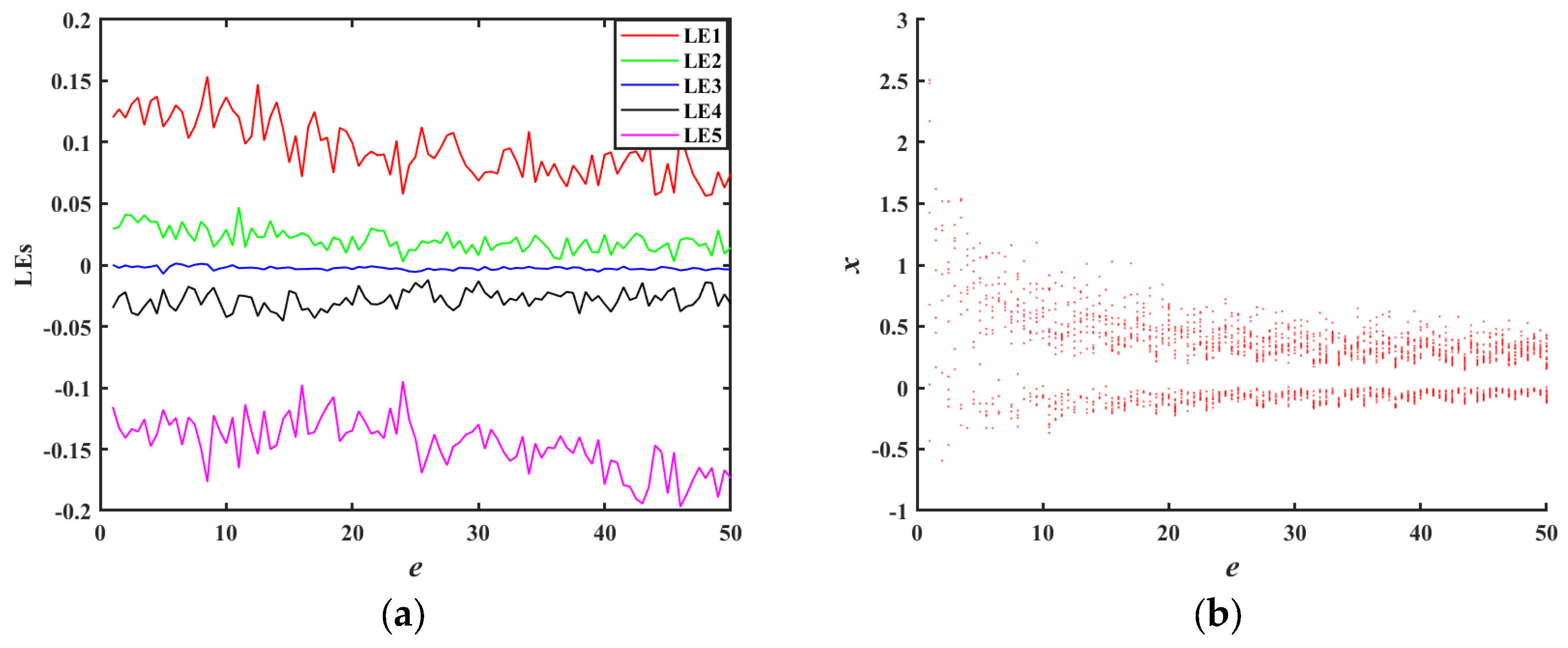
3.1. Large-Scale Hyperchaos Regions

This section explores the system characteristics under chaotic states. Through numerical simulations, system (3) is found to exhibit an exceptionally wide chaotic parameter range. When selecting e as the control variable with system parameters a = 1, b = 1, c = 1, d = 1, q = 0.98 x₀ = 1; y₀ = 1; z₀ = 1; w₀ = 1; u₀ = 1, Figure 13a shows the Lyapunov exponent spectrum (LEs) versus parameter e. The results show that throughout this range, there consistently exists at least one positive Lyapunov exponent. Furthermore, Figure 13b displays the bifurcation diagram of local maxima for variable x versus parameter a, which demonstrates remarkable consistency with the dynamic characteristics revealed by the LEs. The irregular points in the bifurcation diagram correspond well to the chaotic motion observed within this parameter range.

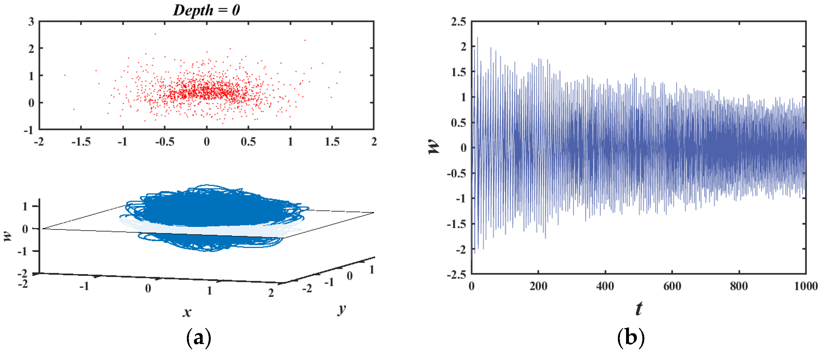
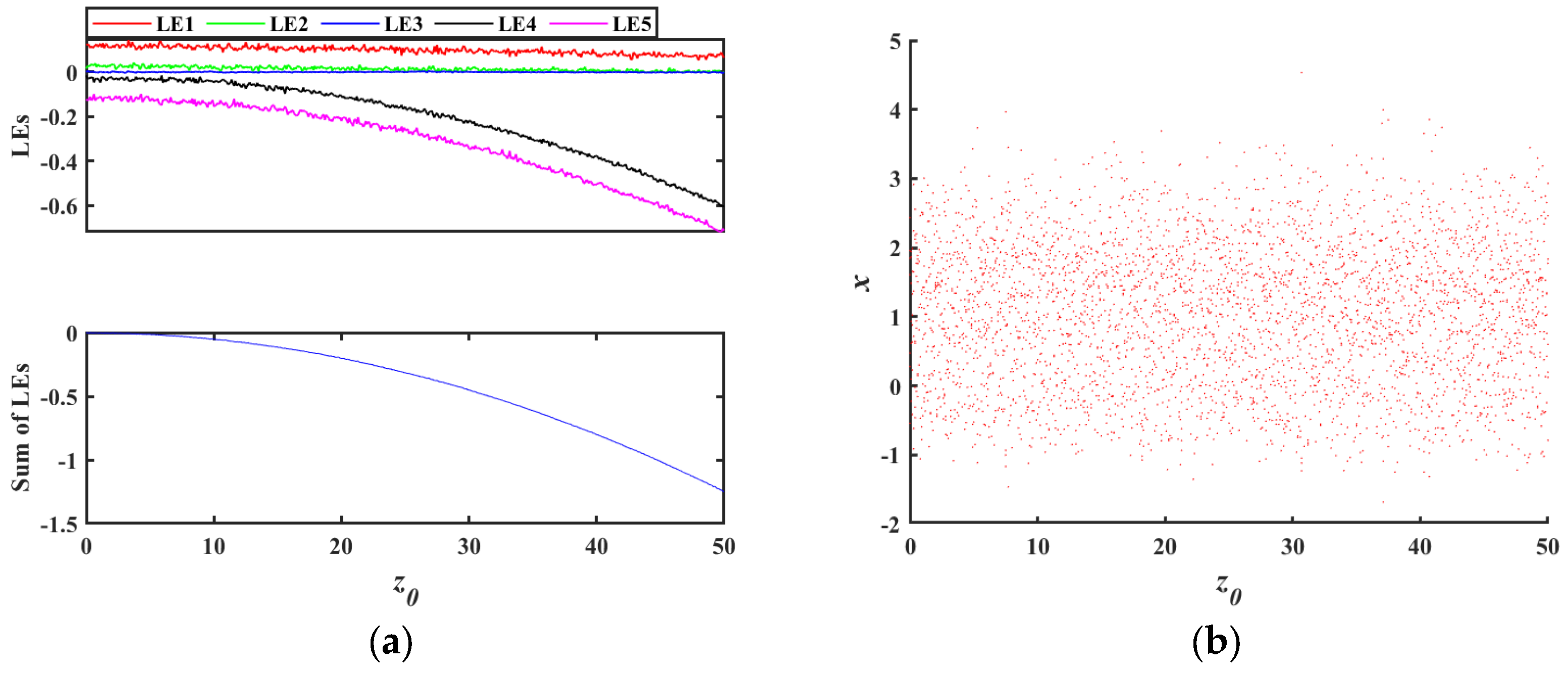
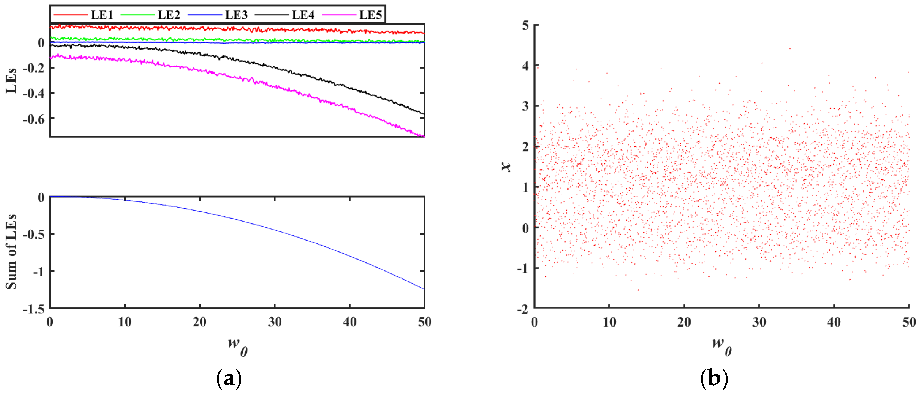
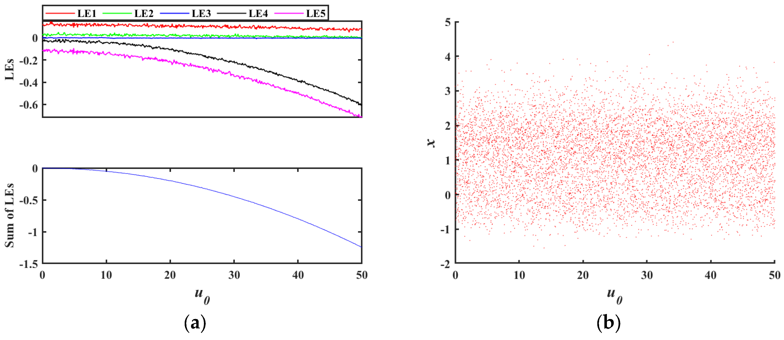
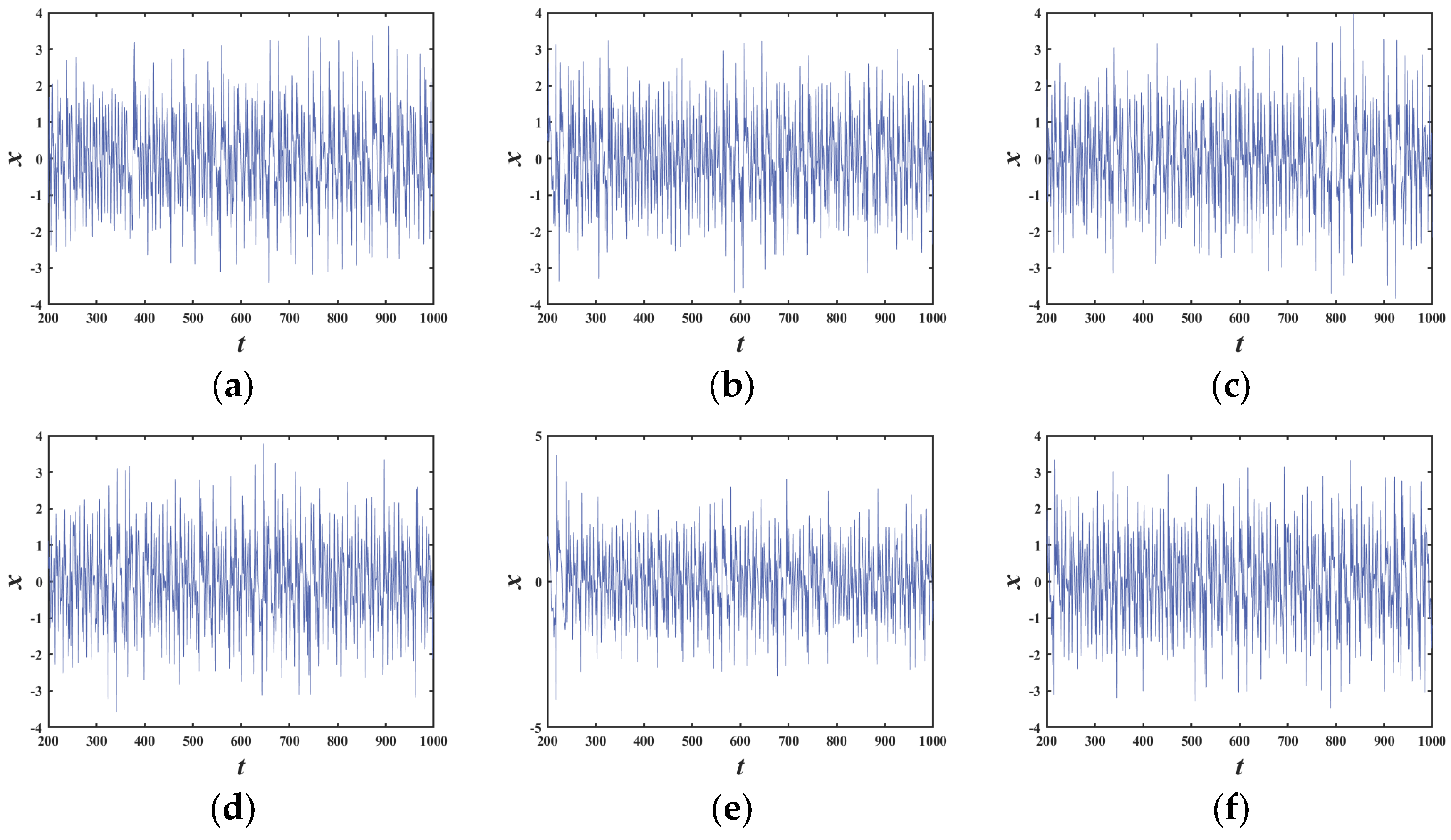
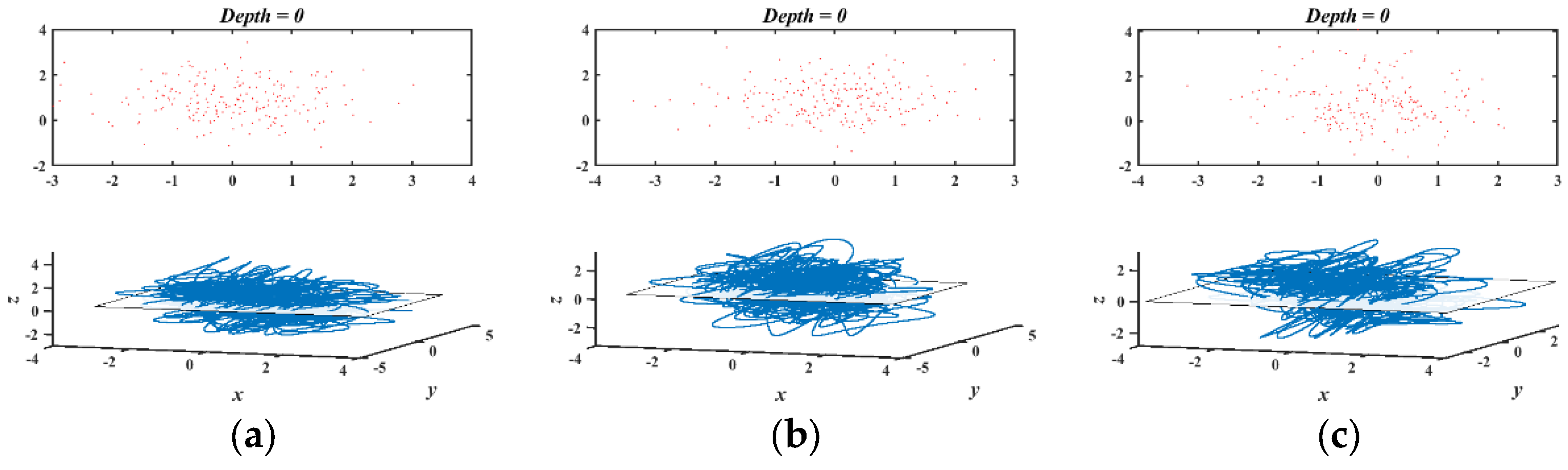
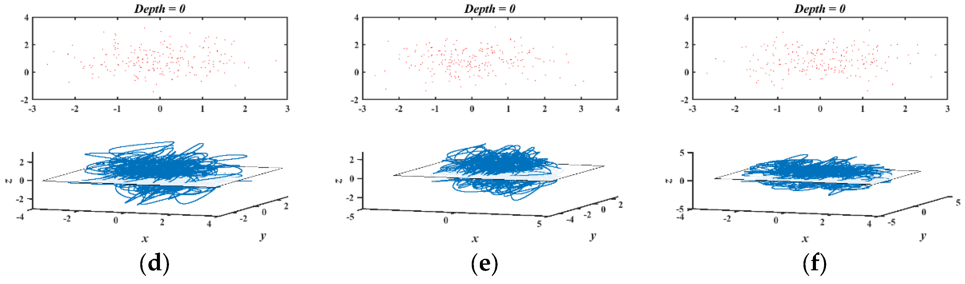
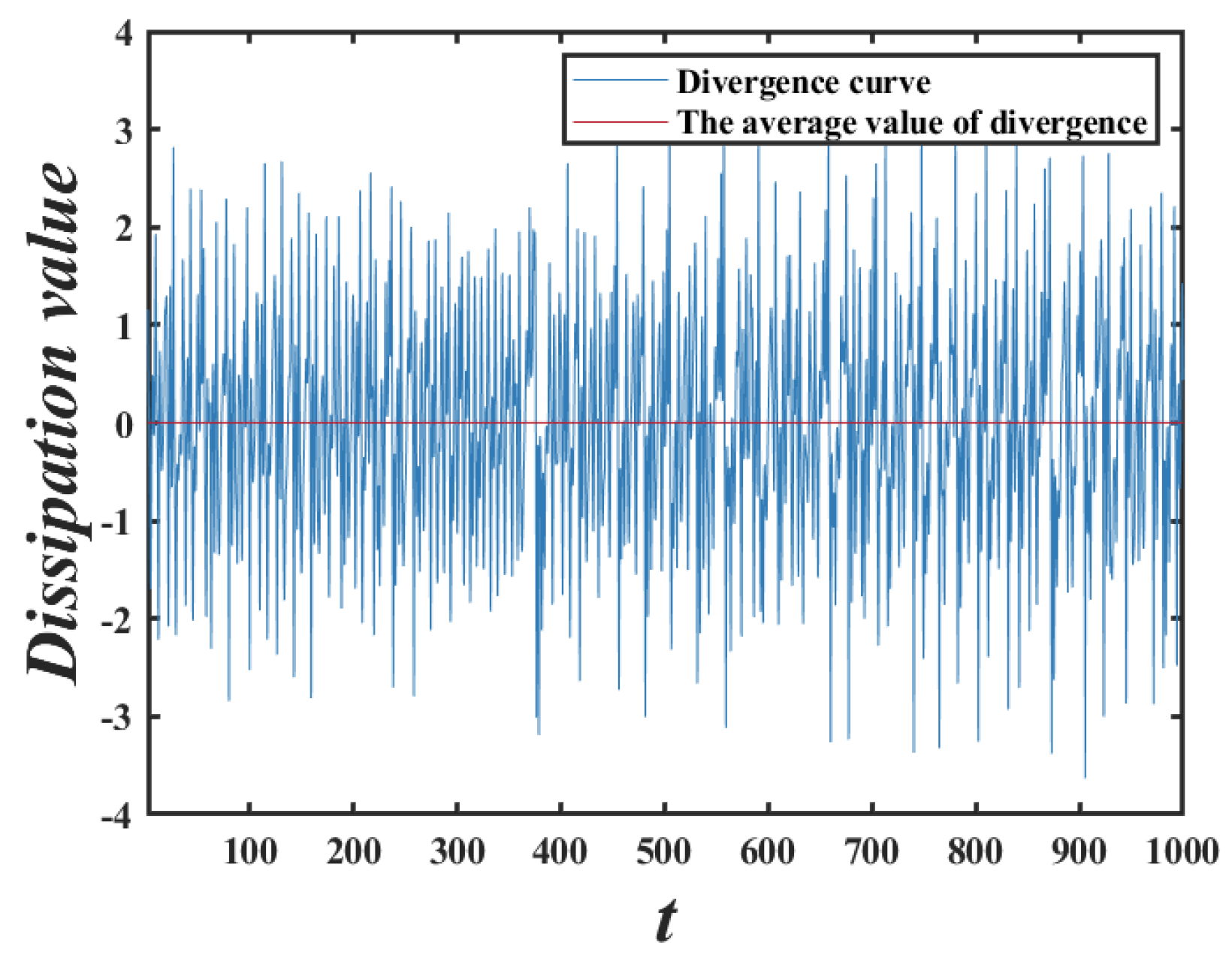
3.2. Transition from Conservative to Dissipative Behavior

This paper further explores system (3) and finds that the large-scale hyperchaotic interval phenomenon also exists for other parameter sets. Under the parameter configuration (a, b, c, d, e, q) = (1, 1, 1, 1, 1, 0.98), the initial values of other non-control variables are set to 1. The bifurcation diagrams and LEs for initial value variations in [0, 50] are shown in Figure 14, Figure 15, Figure 16, Figure 17 and Figure 18. The presence of two positive LEs and irregular points in the bifurcation diagrams indicate hyperchaos without periodic states.

The nature of a nonlinear system can be determined by calculating the sign of the sum of LEs; the relationship between the system’s properties and the sum of LEs is shown in

Table 2. System state and sum of Lyapunov exponent spectra.

Lyapunov Exponent Sum	System Properties
${\displaystyle \sum _i^n}{LE}_i>0$	Divergent
${\displaystyle \sum _i^n}{LE}_i =0$	Conservative
${\displaystyle \sum _i^n}{LE}_i <0$	Dissipative

, where a negative sum indicates dissipativity and a sum of 0 indicates conservativity. Generally, a system can only exhibit one of these properties, either dissipative or conservative. What is rare is that system (3) demonstrates a novel phenomenon: as the initial values change, the overall characteristics of the system switch between dissipativity and conservativity, meaning it possesses both dissipative and conservative properties. As can be seen from the LEs and the sum of all LEs shown from Figure 14a to Figure 18a, the cumulative sum of all LEs initially equals zero (conservative regime). However, with increasing initial values x₀; y₀; z₀; w₀; u₀, the LE sum progressively becomes negative, signifying a dissipative transition. In addition, to more intuitively demonstrate this transformation process, we also plotted the graph of the sum of Lyapunov exponent spectra. Initially, the sum of all LEs equals zero, indicating that the system is conservative at this stage; then, as initial values increase, the LE sum gradually becomes negative, at which point the system demonstrates dissipative behavior. This transitional behavior proves that system (3) undergoes a conservative-to-dissipative transformation.

Meanwhile, to further substantiate the chaotic dynamics examined in Section 3.1 and Section 3.2, we randomly selected some parameters within the chaotic interval and plotted their phase diagrams shown in Figure 19, as well as the Poincaré cross sections and time series diagrams shown in Figure 20 and Figure 21.

Furthermore, based on the dissipation formula (2), we plotted the dissipation curve and the average value of divergence over a period of time for the system under conservative parameters (a, b, c, d, e, q) = (1, 1, 1, 1, 1, 0.98) with initial values (1, 1, 1, 1, 1), as shown in Figure 22. It can be seen that the divergence curve oscillates around the zero axis while the average value of divergence is 0 indicates that the system is conservative under these conditions.

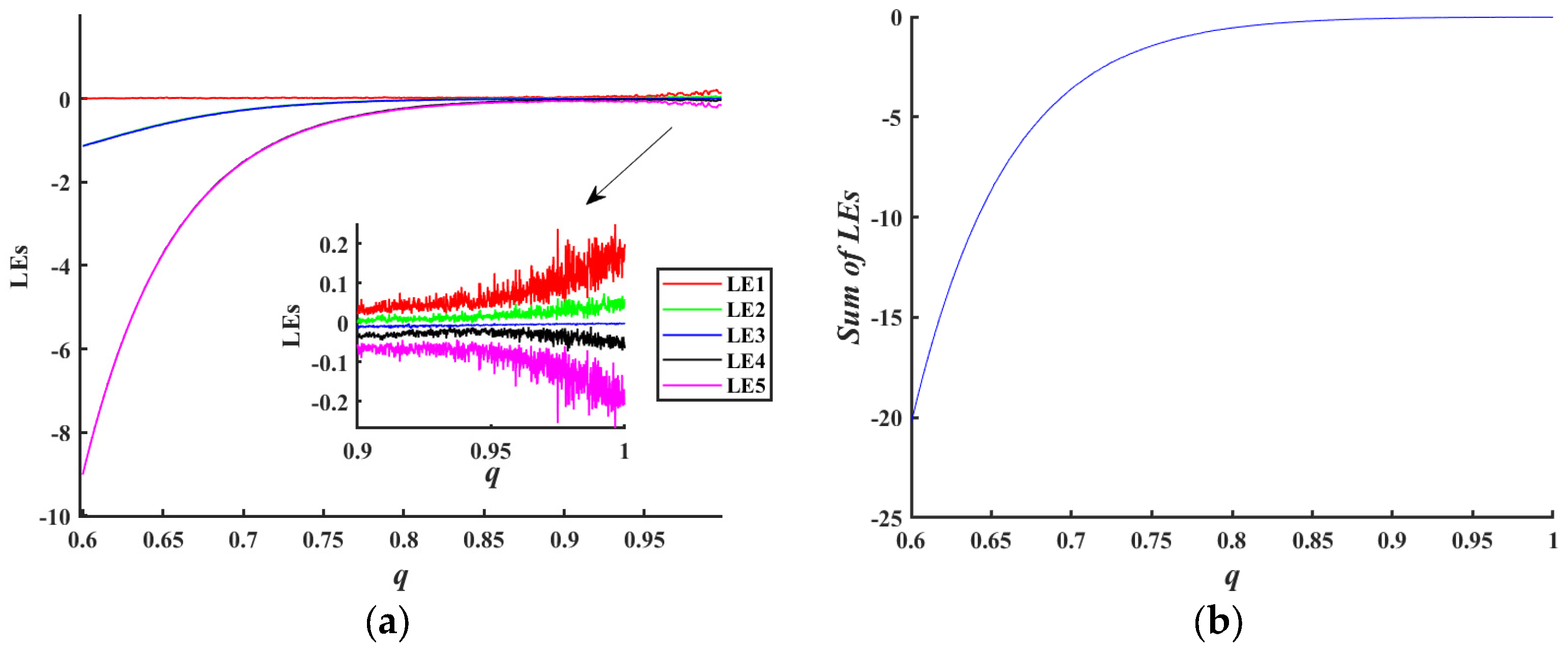
3.3. Fractional-Order Controlled Dynamics

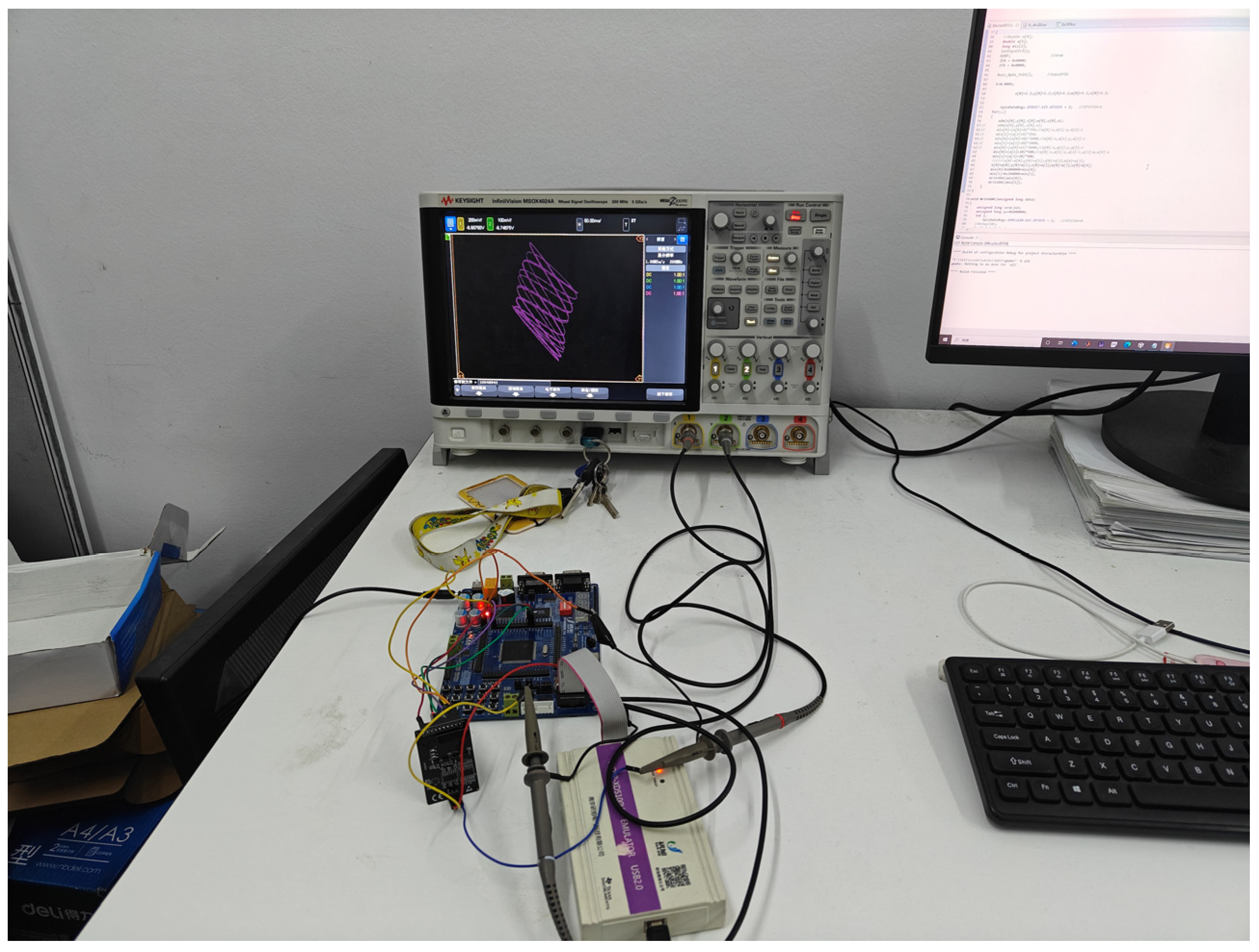
In fractional-order chaotic systems, the q-order can serve as a control variable. Even with identical initial conditions, variations in the numerical value of the fractional-order q can significantly impact the system.

Dissipative to conservative transitions

For system (3), extensive experimental analyses reveal that under the parameter configuration (a, b, c, d, e) = (7, 7, 7, 7, 7) with x₀ = 1.2, y₀ = 1.2; z₀ = 1.2; w₀ = 1.2; u₀ = 1.2. The system undergoes a special transition from dissipative to conservative behavior as the order q of the fractional-order system is altered. It is important to note that q should not be too small; otherwise, the system’s phase trajectories will diverge, losing practical significance. Here, q is set between 0.6 and 1. Figure 23 illustrates the Lyapunov exponents and the sum of all LEs as the system’s order q varies. From the figure, it can be intuitively observed that during the process of q increasing from 0.6 to 1, there is a transition from dissipative to conservative behavior.

A transition behavior related to the order q.

In addition, according to Reference [47], our further research reveals that the system exhibits a unique transient transition behavior related to the order q. When q = 0.7, the system exhibits a clear transition from chaos to quasi-periodicity, as shown in Figure 24a. As q increases to 0.85, this transition weakens and the orbit instead converges to a metastable state that lies between chaos and quasi-periodicity; Figure 24b explicitly illustrates this phenomenon. For q = 0.98, the transitional behavior disappears completely, showing only chaos-to-chaos dynamics, as shown in Figure 24c.

Meanwhile, we further explored whether the integer-order of the system has such a dynamic behavior of transition from a chaotic to a quasi-periodic state under different parameters: under the parameter configuration (a, b, c, d, e, q) = (20, 1, 1, 1, 1, 1) and with initial conditions (35, 1, 1, 1, 1), the system demonstrates chaos-to-chaos transitions, as illustrated in Figure 25a; under the parameter configuration (a, b, c, d, e, q) = (7, 7, 7, 7, 7, 1) with x₀ = 1.2; y₀ = 1.2; z₀ = 1.2; w₀ = 1.2; u₀ = 1.2, the system demonstrates chaos-to-chaos transitions, as illustrated in Figure 25b.

The preceding analysis shows that in the case of integer order, the system does not have the transition from a chaotic to a quasi-periodic state that occurs when the q value is low, which proves that this phenomenon is a unique dynamic behavior of the fractional-order system.

4. DSP Verification

As digital processing technologies like DSP have matured, more chaotic systems are being implemented on DSP experimental platforms [48,49,50]. In this paper, the DSP chip used is the TMS320F28335, which communicates with the external dual-channel DAC8552 via GPIO-emulated SPI protocol. The digital signals are converted to analog signals and displayed as 2D phase diagrams on an oscilloscope. Figure 26 illustrates the overall platform architecture, which comprises three functional layers:

Digital Signal Generation: The DSP solves fractional-order differential equations in real-time using the ADM algorithm. Mixed-Signal Conversion: The DAC8552 provides 16 bit resolution, ensuring minimal phase distortion during analog reconstruction. Dynamics Visualization: An MSOX4024 oscilloscope captures the resulting phase–plane trajectories.

The core control algorithm uses a fifth-order ADM decomposition method to solve system (3) and generate chaotic signals. The program pseudocode is shown in

Table 3. DSP implementation for chaotic system.

Input: State variables x, y, z, w, u; system parameters a, b, c, d, e  Output: Chaotic waveform

1: Configure GPIO pins: GPIO35 as SPI chip select, GPIO36 as SPI clock, GPIO37 as SPI data line. Input initial state variables and parameters. 2: for i = 1 to time do 3: [x_new, y_new, z_new, w_new, u_new] = ADM_Solver (x, y, z, w, u, a, b, c, d, e, h)//Solve differential equations 4: DAC_Ch1 = (y_new + 20) * 500   //Data mapping 5: DAC_Ch2 = (w_new + 20) * 500  //Data mapping 6: SPI_Send(DAC_Ch1, GPIO35, GPIO36, GPIO37) //SPI output, send 24 bit data 7: SPI_Send(DAC_Ch2, GPIO35, GPIO36, GPIO37) //SPI output, send 24 bit data 8: x = x_new; y = y_new; z = z_new; w = w_new; u = u_new//Update state variables 9: end for

.

The SPI_Send function is used to emulate the SPI communication protocol, with pseudocode in

Table 4. SPI communication protocol for DAC signal conversion.

Input: DAC_Ch1, GPIO35, GPIO36, GPIO37  Output: Analog Signal

1: CS = LOW         //Enable chip select 2: for i = 23 down to 0 do //Send data 3: CLK = HIGH 4: MOSI = (data >> i) & 1 //Send current bit 5: CLK = LOW 6: end for 7: CS = HIGH         //Release chip select

. The ADM_Solver function solves system (3), and its pseudocode is in

Table 5. Solution algorithm for system (3).

Input: x0, h, q, a, b, c, d, e  Output: .x_new, y_new, z_new, w_new, u_new

1: c10 = x; c20 = y; c30 =z; c40 = w; c50 = u; 2: c11 = −a* c20+e*c10*c50; 3: c21 = a*c10+b*c30; 4: c31 = −b*c20+c*c40; 5: c41 = −c*c30+d*c50; 6: c51 = 1−d*c40−e*c10*c10; 7: c12 = −a* c21+e*(c11*c50+c10*c51); 8: c22 = a*c11+b*c31; 9: c32 = −b*c21+c*c41; 10: c42 = −c*c31+d*c51; 11: c52 = 1−d*c41−2*e*c10*c11; 12: c13 = −a*c22+e*(c11*c51+c12*c50+c10*c51*(ᴦ(2q+1)/(ᴦ(q+1)^2))); 13: c23 = a*c12+b*c32; 14: c33 = −b*c22+c*c42; 15: c43 = −c*c32+d*c52; 16: c53 = 1−d*c42−e*(2*c10*c12+c11*c11*(ᴦ(2*q+1)/(ᴦ(q+1)^2))); 17: c14 = −a*c23+e*((c11*c52+c12*c51)*(ᴦ(3q+1)/(ᴦ(q+1)* ᴦ(2q+1)))+c10*c53+c13*c50); 18: c24 = a*c13+b*c33; 19: c34 = −b*c23+c*c43; 20: c44 = −c*c33+d*c53; 21: c54 = 1−d*c43−e*(2*c10*c13+2*c12*c11*(ᴦ(3*q+1)/(ᴦ(q+1)* ᴦ(2q+1)))); 22: c15 = −a* c24+e*((c11*c53+c13*c51)*(ᴦ(4q+1)/(ᴦ(q+1)* ᴦ(3q+1)))+c12*c52*(ᴦ(4q+1)/(ᴦ(2q+1)^2))+c10*c54+c14*c50); 23: c25 = a*c14+b*c34; 24: c35 = −b*c24+c*c44; 25: c45 = −c*c34+d*c54; 26: c55 = 1−d*c44−e*(2*c10*c14+2*c13*c11*(ᴦ(4q+1)/(ᴦ(q+1)* ᴦ(3q+1)))+c12*c12*(ᴦ(4q+1)/(ᴦ(2q+1)^2))); 27: x_new(1)= c10+c11*(h^q/ᴦ(q+1))+c12*h^(2*q)/ᴦ(2*q+1)+c13*h^(3*q)/ᴦ(3*q+1)+c14*h^(4*q)/ᴦ(4*q+1)+c15*h^(5*q)/ᴦ(5*q+1); 28: x_new(2)= c20+c21*(h^q/ᴦ(q+1))+c22*h^(2*q)/ᴦ(2*q+1)+c23*h^(3*q)/ᴦ(3*q+1)+c24*h^(4*q)/ᴦ(4*q+1)+c25*h^(5*q)ᴦ(5*q+1); 29: x_new(3)= c30+c31*(h^q/ᴦ(q+1))+c32*h^(2*q)/ᴦ(2*q+1)+c33*h^(3*q)/ᴦ(3*q+1)+c34*h^(4*q)/ᴦ(4*q+1)+c35*h^(5*q)/ᴦ(5*q+1); 30: x_new(4)= c40+c41*(h^q/ᴦ(q+1))+c42*h^(2*q)/ᴦ(2*q+1)+c43*h^(3*q)/ᴦ(3*q+1)+c44*h^(4*q)/ᴦ(4*q+1)+c45*h^(5*q)/ᴦ(5*q+1); 31: x_new(5)= c50+c51*(h^q/ᴦ(q+1))+c52*h^(2*q)/ᴦ(2*q+1)+c53*h^(3*q)/ᴦ(3*q+1)+c54*h^(4*q)/ᴦ(4*q+1)+c55*h^(5*q)/ᴦ(5*q+1); 32: return x_new, y_new, z_new, w_new, u_new

. Note that the numerical range from differential equations differs from the DAC’s required range, so data mapping in lines 4–5 (Table 3) of the program is needed for proper DAC data processing.

The gamma function is denoted by ᴦ. The experimental results show that a step size h = 0.0001 yields optimal phase diagrams for the system.

Figure 27 displays the main circuit for the physical hardware simulation implementation.

Figure 4 displays the phase space trajectory of system (3). The phase diagrams obtained from the DSP experimental platform with identical parameters are shown in Figure 28. A comparison shows that the phase diagrams from system (3) and the oscilloscope are almost identical, confirming the effective implementation of system (3) on the DSP. This demonstrates that system (3) has good physical realizability.

5. Conclusions

This study investigates a five-dimensional fractional-order chaotic system that exhibits exceptionally rich dynamical behaviors through comprehensive numerical simulations and experimental validations. The system demonstrates distinctive features, including phase trajectory offset boosting, rotational dynamics, and contraction phenomena, while its self-regulating amplitude inversion reveals a hidden energy redistribution mechanism, offering new insights into high-dimensional phase-space evolution.

Notably, the system achieves the following:

(1)

Conservative-to-dissipative transitions governed by initial conditions and dissipative-to-conservative transitions controlled by fractional order variations.

(2)

A unique chaotic-to-quasiperiodic transition occurring exclusively at low fractional orders.

Importantly, the signal processing platform, constructed using Digital Signal Processing (DSP) technology, achieves hardware realization. The experimental measurements exhibit remarkable consistency with numerical simulations, validating the system’s physical realizability.

References

1. Lin, H.R.; Wang, C.H.; Tan, Y.M. Hidden Extreme Multistability with Hyperchaos and Transient Chaos in a Hopfield Neural Network Affected by Electromagnetic Radiation. Nonlinear Dyn. 2020, 99, 2369–2386. [Google Scholar] [CrossRef]
2. Bao, H.; Liu, W.B.; Ma, J.; Wu, H.G. Memristor Initial-Offset Boosting in Memristive HR Neuron Model with Hidden Firing Patterns. Int. J. Bifurc. Chaos 2020, 30, 2030029. [Google Scholar] [CrossRef]
3. Sajjadi, S.S.; Baleanu, D.; Jajarmi, A.; Pirouz, H.M. A New Adaptive Synchronization and Hyperchaos Control of a Biological Snap Oscillator. Chaos Solitons Fractals 2020, 138, 109919. [Google Scholar] [CrossRef]
4. Karkaria, B.D.; Manhart, A.; Fedorec, A.J.K.; Barnes, C.P. Chaos in Synthetic Microbial Communities. PLoS Comput. Biol. 2022, 18, e1010548. [Google Scholar] [CrossRef]
5. Signing, V.R.F.; Tegue, G.A.G.; Kountchou, M.; Njitacke, Z.T.; Tsafack, N.; Nkapkop, J.D.D.; Etoundi, C.M.L.; Kengne, J. A Cryptosystem Based on a Chameleon Chaotic System and Dynamic DNA Coding. Chaos Solitons Fractals 2022, 155, 111777. [Google Scholar] [CrossRef]
6. Guler, H. Real-time Fuzzy-pid Synchronization of Memristor-based Chaotic Circuit Using Graphical Coded Algorithm in Secure Communication Applications. Phys. Scr. 2022, 97, 55212. [Google Scholar] [CrossRef]
7. Nasrolahpour, H. Fractional Electromagnetic Metamaterials. Optik 2020, 203, 163969. [Google Scholar] [CrossRef]
8. Gomez-Aguilar, J.F.; Yepez-Martínez, H.; Escobar-Jiménez, R.F.; Astorga-Zaragoza, C.M.; Morales-Mendoza, L.J.; González-Lee, M. Universal Character of the Fractional Space-time Electromagnetic Waves in Dielectric Media. J. Electromagn. Waves Appl. 2015, 29, 727–740. [Google Scholar] [CrossRef]
9. Maurya, R.K.; Devi, V.; Singh, V.K. Multistep Schemes for One and Two Dimensional Electromagnetic Wave Models Based on Fractional Derivative Approximation. J. Comput. Appl. Math. 2020, 380, 112985. [Google Scholar] [CrossRef]
10. El-Saka, H.A.A.; Lee, S.; Jang, B. Dynamic Analysis of Fractional-order Predator-prey Biological Economic System with Holling Type II Functional Response. Nonlinear Dyn. 2019, 96, 407–416. [Google Scholar] [CrossRef]
11. Ramesh, P.; Sambath, M.; Mohd, H.M.; Krishnan, B. Stability Analysis of the Fractional-order Prey-predator Model with Infection. Int. J. Model. Simul. 2020, 41, 434–450. [Google Scholar] [CrossRef]
12. Wang, J.; Lee, M.C.; Kim, J.H.; Kim, H.H. Fast Fractional-Order Terminal Sliding Mode Control for Seven-Axis Robot Manipulator. Appl. Sci. 2020, 10, 7757. [Google Scholar] [CrossRef]
13. Saad, F.; Belafhal, A. Propagation Properties of Hollow Higher-order Cosh-Gaussian Beams in Quadratic Index Medium and Fractional Fourier Transform. Opt. Quantum Electron. 2021, 53, 28. [Google Scholar] [CrossRef]
14. Mystkowski, A.; Zolotas, A. PLC-based Discrete Fractional-order Control Design for an Industrial-oriented Water Tank Volume System with Input Delay. Fract. Calc. Appl. Anal. 2018, 21, 1005–1026. [Google Scholar] [CrossRef]
15. Li, Y.; Wang, H.P.; Tian, Y. Fractional-order Adaptive Controller for Chaotic Synchronization and Application to a Dual-channel Secure Communication System. Mod. Phys. Lett. B 2019, 33, 1950290. [Google Scholar] [CrossRef]
16. Rivero, M.; Trujillo, J.J.; Vázquez, L.; Velasco, M.P. Fractional Dynamics of Populations. Appl. Math. Comput. 2011, 218, 1089–1095. [Google Scholar] [CrossRef]
17. Vaidyanathan, S.; Pakiriswamy, S. A 3-D Novel Conservative Chaotic System and Its Generalized Projective Synchronization via Adaptive Control. J. Eng. Sci. Technol. Rev. 2014, 8, 52–60. [Google Scholar] [CrossRef]
18. Vaidyanathan, S.; Volos, C. Analysis and Adaptive Control of a Novel 3-D Conservative No-equilibrium Chaotic System. Arch. Control Sci. 2015, 25, 333–353. [Google Scholar] [CrossRef]
19. Cang, S.J.; Wu, A.G.; Wang, Z.H.; Chen, Z.Q. Four-dimensional Autonomous Dynamical Systems with Conservative Flows: Two-case Study. Nonlinear Dyn. 2017, 89, 2495–2508. [Google Scholar] [CrossRef]
20. Jafari, S.; Nazarimehr, F.; Sprott, J.C.; Golpayegani, S.M.R.H. Limitation of Perpetual Points for Confirming Conservation in Dynamical Systems. Int. J. Bifurc. Chaos 2015, 25, 1550182. [Google Scholar] [CrossRef]
21. Prasad, A. Existence of Perpetual Points in Nonlinear Dynamical Systems and Its Applications. Int. J. Bifurc. Chaos 2015, 25, 1530005. [Google Scholar] [CrossRef]
22. Wu, A.G.; Cang, S.J.; Zhang, R.Y.; Wang, Z.; Chen, Z. Hyperchaos in a Conservative System with Nonhyperbolic Fixed Points. Complexity 2018, 2018, 9430637. [Google Scholar] [CrossRef]
23. Cang, S.J.; Wu, A.G.; Zhang, R.Y.; Wang, Z.; Chen, Z. Conservative Chaos in a Class of Nonconservative Systems: Theoretical Analysis and Numerical Demonstrations. Int. J. Bifurc. Chaos 2018, 28, 1850087. [Google Scholar] [CrossRef]
24. Singh, J.P.; Roy, B.K. Five New 4-D Autonomous Conservative Chaotic Systems with Various Type of Non-Hyperbolic and Lines of Equilibria. Chaos Solitons Fractals 2018, 114, 81–91. [Google Scholar] [CrossRef]
25. Gu, S.Q.; Du, B.X.; Wan, Y.J. A New Four-Dimensional Non-Hamiltonian Conservative Hyperchaotic System. Int. J. Bifurc. Chaos 2020, 30, 2050242. [Google Scholar] [CrossRef]
26. Zhang, Z.; Huang, L.; Liu, J.; Guo, Q.; Du, X. A new method of constructing cyclic symmetric conservative chaotic systems and improved offset boosting control. Chaos Solitons Fractals 2022, 158, 112103. [Google Scholar] [CrossRef]
27. Ke, Y.Q.; Miao, C.F. Mittag-Leffler Stability of Fractional-order Lorenz and Lorenz-family Systems. Nonlinear Dyn. 2016, 83, 1237–1246. [Google Scholar] [CrossRef]
28. Azil, S.; Odibat, Z.; Shawagfeh, N. Nonlinear Dynamics and Chaos in Caputo-Like Discrete Fractional Chen System. Phys. Scr. 2021, 96, 95219. [Google Scholar] [CrossRef]
29. Odibat, Z.; Corson, N.; Aziz-Alaoui, M.A.; Alsaedi, A. Chaos in Fractional Order Cubic Chua System and Synchronization. Int. J. Bifurc. Chaos 2017, 27, 1750161. [Google Scholar] [CrossRef]
30. Jia, H.Y.; Chen, Z.Q.; Qi, G.Y. Topological Horseshoe Analysis and Circuit Realization for a Fractional-Order Lü System. Nonlinear Dyn. 2013, 74, 203–212. [Google Scholar] [CrossRef]
31. Xu, C.J.; Liao, M.X.; Li, P.L.; Yao, L.; Qin, Q.; Shang, Y. Chaos Control for a Fractional-Order Jerk System via Time Delay Feedback Controller and Mixed Controller. Fractal Fract. 2021, 5, 257. [Google Scholar] [CrossRef]
32. Cafagna, D.; Grassi, G. Fractional-Order Systems without Equilibria: The First Example of Hyperchaos and Its Application to Synchronization. Chin. Phys. B 2015, 24, 80502. [Google Scholar] [CrossRef]
33. Zhang, S.; Zeng, Y.C.; Li, Z.J.; Zhou, C.Y. Hidden Extreme Multistability, Antimonotonicity and Offset Boosting Control in a Novel Fractional-Order Hyperchaotic System Without Equilibrium. Int. J. Bifurc. Chaos 2018, 28, 1850167. [Google Scholar] [CrossRef]
34. Leng, X.; Gu, S.; Peng, Q.; Du, B. Study on a four-dimensional fractional-order system with dissipative and conservative properties. Chaos Solitons Fractals 2021, 150, 111185. [Google Scholar] [CrossRef]
35. Tian, B.; Peng, Q.; Leng, X.; Du, B. A new 5D fractional-order conservative hyperchaos system. Phys. Scr. 2022, 98, 15207. [Google Scholar] [CrossRef]
36. Leng, X.; Zhang, C.; Du, B. Modeling methods and characteristic analysis of new Hamiltonian and non-Hamiltonian conservative chaotic systems. AEU-Int. J. Electron. Commun. 2022, 152, 154242. [Google Scholar] [CrossRef]
37. Zhou, L.; Wang, C.H.; Zhang, X.; Yao, W. Various Attractors, Coexisting Attractors and Antimonotonicity in a Simple Fourth-Order Memristive Twin-T Oscillator. Int. J. Bifurc. Chaos 2018, 28, 1850050. [Google Scholar] [CrossRef]
38. Leng, X.; Zhang, L.; Zhang, C.; Du, B. Modeling and complexity analysis of a fractional-order memristor conservative chaotic system. Phys. Scr. 2023, 98, 75206. [Google Scholar] [CrossRef]
39. Lenka, B.K.; Upadhyay, R.K. New globally Lipschitz no-equilibrium fractional order systems and control of hidden memory chaotic attractors. J. Comput. Sci. 2025, 88, 102603. [Google Scholar] [CrossRef]
40. Xiangxin, L.; Baoxiang, D.; Shuangquan, G.; He, S. Novel dynamical behaviors in fractional-order conservative hyperchaotic system and DSP implementation. Nonlinear Dyn. 2022, 109, 1167–1186. [Google Scholar] [CrossRef]
41. Ye, X.L.; Wang, X.Y. Characteristic Analysis of a Simple Fractional-Order Chaotic System with Infinitely Many Coexisting Attractors and Its DSP Implementation. Phys. Scr. 2020, 95, 75212. [Google Scholar] [CrossRef]
42. Fu, H.Y.; Lei, T.F. Adomian Decomposition, Dynamic Analysis and Circuit Implementation of a 5D Fractional-Order Hyperchaotic System. Symmetry 2022, 14, 484. [Google Scholar] [CrossRef]
43. Rajagopal, K.; Nazarimehr, F.; Karthikeyan, A.; Srinivasan, A.; Jafari, S. CAMO: Self-Excited and Hidden Chaotic Flows. Int. J. Bifurc. Chaos 2019, 29, 1950143. [Google Scholar] [CrossRef]
44. Li, G.H.; Zhang, X.Y.; Yang, H. Complexity Analysis and Synchronization Control of Fractional-Order Jafari-Sprott Chaotic System. IEEE Access 2020, 8, 53360–53373. [Google Scholar] [CrossRef]
45. Yang, F.F.; Li, P. Characteristics Analysis of the Fractional-Order Chaotic Memristive Circuit Based on Chua’s Circuit. Mob. Netw. Appl. 2019, 26, 1862–1870. [Google Scholar] [CrossRef]
46. He, S.B.; Sun, K.H.; Wang, H.H. Dynamics and Synchronization of Conformable Fractional-Order Hyperchaotic Systems Using the Homotopy Analysis Method. Commun. Nonlinear Sci. Numer. Simul. 2019, 73, 146–164. [Google Scholar] [CrossRef]
47. Lenka, B.K.; Upadhyay, R.K. Hidden memory chaotic attractors in simple nonequilibrium fractional order systems. Commun. Nonlinear Sci. Numer. Simul. 2025, 150, 108970. [Google Scholar] [CrossRef]
48. Fan, Z.; Zhang, C.; Wang, Y.; Du, B. Construction, dynamic analysis and DSP implementation of a novel 3D discrete memristive hyperchaotic map. Chaos Solitons Fractals 2023, 177, 114303. [Google Scholar] [CrossRef]
49. Liu, B.; Ye, X.L.; Hu, G. Design of a New 3D Chaotic System Producing Infinitely Many Coexisting Attractors and Its Application to Weak Signal Detection. Int. J. Bifurc. Chaos 2021, 31, 2150235. [Google Scholar] [CrossRef]
50. Yang, F.F.; Mou, J.; Ma, C.G.; Cao, Y.H. Dynamic Analysis of an Improper Fractional-Order Laser Chaotic System and Its Image Encryption Application. Opt. Lasers Eng. 2020, 129, 106031. [Google Scholar] [CrossRef]
Figure 1. Five-dimensional systems within cryptographic algorithms.
Mathematics 13 02477 g001
Figure 2. Adomian Decomposition Method. (ac) Phase diagram in wu, yz, and zw planes.
Mathematics 13 02477 g002
Figure 3. Runge–Kutta decomposition method. (ac) Phase diagram in wu, yz, and zw planes.
Mathematics 13 02477 g003
Figure 4. Phase diagram. (ac) Quasi-periodic motions in xw, xu, and yw planes. (df) Corresponding chaotic attractors in the same projection planes.
Mathematics 13 02477 g004
Figure 5. Three-dimensional phase diagram and Poincaré cross sections and timing diagram of system in a quasi-periodic state. (a) Three-dimensional phase diagram, Poincaré cross sections (b) The timing diagram.
Mathematics 13 02477 g005
Figure 6. Three-dimensional phase diagram, Poincaré cross sections and timing diagram of system in a chaotic state.(a) Three-dimensional phase diagram, Poincaré cross sections (b) The timing diagram.
Mathematics 13 02477 g006
Figure 7. The offset boost behavior of the phase trajectory; x0 = 30, 35, 40, 45, 50.
Mathematics 13 02477 g007
Figure 8. The average with x0.
Mathematics 13 02477 g008
Figure 9. The rotation behavior of the phase trajectory: (a) c = −2, 0, 2, 4; (b) c = 21, 22, 23, 24.
Mathematics 13 02477 g009
Figure 10. The contraction behavior of the phase trajectory: (a) c = 1, 2, 3, 4, 5; (b) d = 42, 44, 46, 48, 50.
Mathematics 13 02477 g010
Figure 11. Phase trajectories varying with x3.
Mathematics 13 02477 g011
Figure 12. Phase trajectories of x3 under different times: (a) t ∈ [0s, 2.6s]; (b) t ∈ [5s, 100s].
Mathematics 13 02477 g012
Figure 13. Dynamical behavior analysis. (a) LE1-LE5 versus parameter e. (b) Bifurcation diagram versus parameter e.
Mathematics 13 02477 g013
Figure 14. Dynamic behavior analysis through Lyapunov exponent sum of LEs and bifurcation diagram. (a) (Top) Lyapunov exponent spectrum (LE1–LE5) versus initial condition x0. (Bottom) Corresponding Lyapunov exponent sum (ΣLEs). (b) Bifurcation diagram versus initial condition x0.
Mathematics 13 02477 g014
Figure 15. Dynamic behavior analysis through Lyapunov exponent sum of LEs and bifurcation diagram. (a) (Top) Lyapunov exponent spectrum (LE1-LE5) versus initial condition y0. (Bottom) Corresponding Lyapunov exponent sum (ΣLEs). (b) Bifurcation diagram versus initial condition y0.
Mathematics 13 02477 g015
Figure 16. Dynamic behavior analysis through Lyapunov exponent sum of LEs and bifurcation diagram. (a) (Top) Lyapunov exponent spectrum (LE1-LE5) versus initial condition z0. (Bottom) Corresponding Lyapunov exponent sum (ΣLEs). (b) Bifurcation diagram versus initial condition z0.
Mathematics 13 02477 g016
Figure 17. Dynamic behavior analysis through Lyapunov exponent sum of LEs and bifurcation diagram. (a) (Top) Lyapunov exponent spectrum (LE1-LE5) versus initial condition w0. (Bottom) Corresponding Lyapunov exponent sum (ΣLEs). (b) Bifurcation diagram versus initial condition w0.
Mathematics 13 02477 g017
Figure 18. Dynamic behavior analysis through Lyapunov exponent sum of LEs and bifurcation diagram. (a) (Top) Lyapunov exponent spectrum (LE1-LE5) versus initial condition u0. (Bottom) Corresponding Lyapunov exponent sum (ΣLEs). (b) Bifurcation diagram versus initial condition u0.
Mathematics 13 02477 g018
Figure 19. Phase diagrams under different parameters: (a) e = 1; (b) x0 = 6.5; (c) y0 = 29.1; (d) z0 = 13.8; (e) w0 = 44.3; (f) u0 = 31.8.
Mathematics 13 02477 g019
Figure 20. The timing diagram under different parameters: (a) e = 1; (b) x0 = 6.5; (c) y0 = 29.1; (d) z0 = 13.8; (e) w0 = 44.3; (f) u0 = 31.8.
Mathematics 13 02477 g020
Figure 21. Three-dimensional phase diagram and Poincaré cross sections under different parameters: (a) e = 1; (b) x0 = 6.5; (c) y0 = 29.1; (d) z0 = 13.8; (e) w0 = 44.3; (f) u0 = 31.8.
Mathematics 13 02477 g021aMathematics 13 02477 g021b
Figure 22. The system divergence curve and the average value of divergence.
Mathematics 13 02477 g022
Figure 23. Dynamical behavior analysis through Lyapunov exponent sum of LEs and bifurcation diagram. (a) Lyapunov exponent spectrum (LE1-LE5) versus parameter q. (b) Corresponding Lyapunov exponent sum (ΣLEs).
Mathematics 13 02477 g023
Figure 24. Transient phenomena observed in the system under different fractional orders: (a) q = 0.7; (b) q = 0.85; (c) q = 0.98.
Mathematics 13 02477 g024
Figure 25. The transient behaviors of integer-order systems (a) (a, b, c, d, e, q) = (20, 1, 1, 1, 1, 1) initial conditions (35, 1, 1, 1, 1); (b) (a, b, c, d, e, q) = (7, 7, 7, 7, 7, 1) initial conditions (1.2, 1.2, 1.2, 1.2, 1.2).
Mathematics 13 02477 g025
Figure 26. Hardware platform design diagram.
Mathematics 13 02477 g026
Figure 27. Hardware photograph of system (3) implemented on DSP.
Mathematics 13 02477 g027
Figure 28. DSP platform realizes the phase diagram of each part of the system. (ac) Quasi-periodic motions in xw, xu, and yw planes. (df) Corresponding chaotic attractors in the same projection planes.
Mathematics 13 02477 g028