Real Reactive Micropolar Spherically Symmetric Fluid Flow and Thermal Explosion: Modelling and Existence

Abstract

A model for the flow and thermal explosion of a micropolar gas is investigated, assuming the equation of state for a real gas. This model describes the dynamics of a gas mixture (fuel and oxidant) undergoing a one-step irreversible chemical reaction. The real gas model is particularly suitable in this context because it more accurately reflects reality under extreme conditions, such as high temperatures and high pressures. Micropolarity introduces local rotational dynamic effects of particles dispersed within the gas mixture. In this paper, we first derive the initial-boundary value system of partial differential equations (PDEs) under the assumption of spherical symmetry and homogeneous boundary conditions. We explain the underlying physical relationships and then construct a corresponding approximate system of ordinary differential equations (ODEs) using the Faedo–Galerkin projection. The existence of solutions for the full PDE model is established by analyzing the limit of the solutions of the ODE system using a priori estimates and compactness theory. Additionally, we propose a numerical scheme for the problem based on the same approximate system. Finally, numerical simulations are performed and discussed in both physical and mathematical contexts.

1. Introduction

Reactive compressible fluid models describe the behavior of fluids in which chemical reactions occur simultaneously with compressible flow dynamics, often coupled with heat transfer and diffusion effects. These models extend classical compressible fluid frameworks by incorporating additional variables and source terms to account for reaction kinetics and energy release, making the governing equations highly nonlinear and tightly coupled [1,2]. Reversible and irreversible processes that comply with the laws of thermodynamics and continuum mechanics are often modelled. Foundational work on reactive compressible fluids [3] have laid out the governing equations for compressible reactive flows including the conservation of mass, momentum, energy, and fuel quantity. These models are crucial for accurately describing phenomena like combustion, thermal explosions, and chemically driven instabilities in gases.

Symmetric fluid models, such as those assuming spherical or cylindrical symmetry, play a significant role in simplifying and analyzing complex fluid flow problems by reducing the spatial dimensionality while preserving essential physical features. In the context of compressible fluids, spherical symmetry implies that all flow variables depend solely on the radial coordinate and time. This assumption is particularly useful in modelling phenomena like thermal explosions, bubble dynamics, or astrophysical flows, where the geometry naturally suggests a radially symmetric configuration [4,5,6,7]. Cylindrical symmetry, on the other hand, assumes invariance along the azimuthal angle and is relevant for capturing effects in pipe flows, jets, or rotating systems [8].

The real micropolar gas model extends classical fluid dynamics by incorporating both the microstructural effects of micropolar fluids [9,10] and the non-ideal behavior of real gases [1,11]. Unlike ideal gases, a real gas model gives a generalization which is suitable for describing extreme situations such as high pressure, which can be expected in reactive fluid frameworks. The micropolar aspect introduces additional degrees of freedom related to the rotation of fluid particles and coupled stresses, capturing micro-rotational inertia and spin viscosity effects that are absent in classical Navier–Stokes models. This combination results in a system of nonlinear partial differential equations that describe the conservation of mass, momentum, energy, and microrotation. Additionally, micropolar real reactive models also account for reactive dynamics, reflecting the complex interplay between compressibility, microstructures, thermal conduction, and chemical reactions.

Recent studies [12,13,14,15,16] have rigorously analyzed one-dimensional viscous, thermally conductive micropolar real gas flows with reactive terms, proving the local existence of generalized solutions and developing numerical schemes to approximate them. Such models are essential for accurately describing phenomena like thermal explosions and reactive flows in gases where both microstructural effects and deviations from the ideal gas behavior are significant, providing a more realistic and comprehensive framework compared to classical fluid models.

Similar models have also been studied in recent years. For example, in [17,18], the authors studied a real, non-reactive micropolar gas in one spatial dimension. In [4], the author investigated global spherically symmetric solutions to the ideal gas, as well as a non-reactive, non-micropolar model in an exterior domain, and in [5,6,19], the authors investigated the existence of and numerical methods for solutions to the spherically symmetric model of an ideal, non-reactive, micropolar gas in three spatial dimensions. In [20], the author studied the uniqueness of the solution to the shear flow problem for a compressible viscous micropolar fluid. In [21], the authors derived global a priori estimates for a viscous reactive non-micropolar gas. In [22,23,24,25,26], the authors studied a model of a real non-micropolar gas, and in [1,2], they considered a model of a real reactive non-micropolar gas. In [27], a spherically symmetric model for a real non-reactive micropolar gas was derived and studied numerically. Magneto-micropolar gases have also been studied recently; for instance, in [28], the authors considered the Cauchy problem for three-dimensional compressible magneto-micropolar fluids with vacuum, and in [29], they examined spherical particles immersed in an unbounded magneto-micropolar fluid. In [30], the authors reviewed investigations on the unsteady flow and heat transfer of micropolar fluids, boundary layers, their thermophysical properties, and their thermodynamic and hydrodynamic behavior, while in [31], they developed an analytical approach for micropolar fluid flow in a channel with porous walls. In [32], the axisymmetric creeping flow of a micropolar fluid past a porous surface saturated with micropolar fluid is investigated analytically. In [33], the authors studied a blood flow model using the micropolar fluid framework.

This paper focuses on the mathematical modelling and analysis of spherically three-dimensional symmetric flow and thermal explosion in a real micropolar reactive gas. To the best of our knowledge, this specific model has not been studied previously, only its one-dimensional counterpart. The aim is to achieve three goals. First, we derive a spherically symmetric model of reactive micropolar real gas flow and thermal explosion in mass Lagrangian coordinates. To achieve this, we choose a spherically symmetric domain and assume spherical symmetry for the solution. Second, we prove that a solution to the derived model exists locally in time. For this, we construct an approximation scheme based on the Faedo–Galerkin method and show the convergence of the approximate solutions to a solution of our problem using a priori estimates and compactness theory. Finally, we use the same Faedo–Galerkin approximations as a basis for deriving a numerical scheme and conducting numerical experiments. The main difficulty lies in addressing the analytical and computational challenges posed by the nonlinearities in the system. The proposed approach not only facilitates the analytical proof of the local existence of generalized solutions but also provides a practical tool for numerical simulations. Through this study, we aim to deepen the theoretical understanding of micropolar reactive gas flows and establish reliable computational methods to study their dynamic behavior.

The paper is structured as follows: In the second section, we derive the governing initial-boundary value problem with homogeneous boundary conditions. In the third, we state the local existence theorem, and in the fourth, we construct an approximate problem using Faedo–Galerkin projections. In the fifth, we prove the local existence theorem by obtaining a priori estimates for the constructed approximate solutions, and in the sixth, we use this construction to solve the problem numerically and verify the model.

Nomenclature

This section presents the notation used throughout the paper for clarity and ease of understanding.

• $\rho =\rho (x,t)$ is mass density, and ${\rho }_0={\rho }_0\left(x\right)$ is the initial mass density;
• $v=v(x,t)$ is velocity, and $v_0=v_0\left(x\right)$ is the initial velocity;
• $P=P(x,t)$ is pressure;
• $\omega =\omega (x,t)$ is microrotational velocity, and ${\omega }_0={\omega }_0\left(x\right)$ is the initial microrotational velocity;
• $\theta =\theta (x,t)$ is absolute temperature, and ${\theta }_0={\theta }_0\left(x\right)$ is the initial absolute temperature;
• $z=z(x,t)$ is the concentration of unburned fuel, and $z_0=z_0\left(x\right)$ is the initial concentration of unburned fuel;
• $r=r(x,t)$ is the function connecting Eulerian spatial coordinate r and mass Lagrangian spatial coordinate x, and $r_0=r_0\left(x\right)$ the value of r at the initial moment;
• $L>0$ is a constant that appeared during conversion from Eulerian to Lagrangian coordinates;
• $\lambda$ is the second viscosity coefficient;
• $\mu$ is the dynamic Newtonian viscosity;
• ${\mu }_r$ is the dynamic microrotation viscosity;
• $c_0$ and $c_d$ are the coefficients of angular viscosities;
• $j_I>0$ is the microinertia coefficient;
• $c_v>0$ is the specific heat at constant volume;
• $\kappa >0$ is the heat conductivity coefficient;
• $\sigma >0$ is the species diffusion coefficient;
• $\delta >0$ is the reaction rate;
• $I=I(\rho ,\theta ,z)$ is the intensity of the chemical reaction;
• C, $C_i$ are generic positive constants;
• n determines the dimension of the finite-dimensional space from which approximations $f^n$, $f\in \{\rho ,v,\omega ,\theta ,z,r\}$ are constructed.

2. Modelling

2.1. Real Reactive Micropolar Fluid

The model we are interested in in this study is built upon a classical compressible Navier–Stokes system of partial differential equations with temperature, namely the laws of conservation of mass, momentum, and energy [34].

$$\begin{array}{c}\hfill \begin{array}{cc}\hfill & \dot{\rho }+\nabla ·\left(\rho \mathbf{v}\right)=0\hfill \\ \hfill & \rho \dot{\mathit{v}}=\nabla ·\mathit{T}+\rho \mathit{f}\hfill \\ \hfill & \rho \dot{E}=-\nabla ·\mathit{q}+\mathit{T}:\nabla \mathit{v}\hfill \end{array}\end{array}$$

(1)

where $\rho$ is the mass density, $\mathbf{v}$ is the velocity, $\mathit{T}$ is the stress tensor, $\mathit{f}$ is the body force, E is the internal energy, and $\mathit{q}$ is the heat flux. We also incorporate the assumptions of thermodynamic polytropy and thermal conductivity i.e., Fourier’s law [34].

$$\begin{array}{c}\hfill \begin{array}{cc}\hfill & E=c_v\theta \hfill \\ \hfill & \mathit{q}=-\kappa \nabla \theta \hfill \end{array}\end{array}$$

(2)

where $\theta$ is the absolute temperature.

The micropolar fluid model additionally takes into account the microrotational velocity $\mathit{\omega }$, which describes local micro-effects in the fluid. The following corrections are made to the classical system in order to incorporate micropolarity into the model [9,34]:

• The stress tensor is given by

  $${\mathit{T}}_{ij}=(-P+\lambda {\mathit{v}}_{k,k}){\delta }_{ij}+\mu \left({\mathit{v}}_{i,j}+{\mathit{v}}_{j,i}\right)+{\mu }_r\left({\mathit{v}}_{j,i}-{\mathit{v}}_{i,j}\right)-2{\mu }_r{\epsilon }_{mij}{\mathit{\omega }}_m,$$

  (3)

  where ${\mu }_r$, $c_0$, $c_d$, and $c_a$ are coefficients of microviscosity. Notice that $\mathit{T}$ is not symmetric like in the classical case.
• Due to non-symmetry of the stress tensor, the law of conservation of the angular momentum equation is not implied by the conservation of mass and momentum and needs to be added to the model.

  $$j_I\rho \dot{\mathit{\omega }}=\nabla ·\mathit{C}+{\mathit{T}}_x+\rho \mathit{g},$$

  (4)

  where $j_I$ is microinertia density and $\mathit{C}$ is the coupled stress tensor.

  $${\mathit{C}}_{ij}=c_0{\mathit{\omega }}_{k,k}{\delta }_{ij}+c_d\left({\mathit{\omega }}_{i,j}+{\mathit{\omega }}_{j,i}\right)+c_a\left({\mathit{\omega }}_{j,i}-{\mathit{\omega }}_{i,j}\right)$$

  (5)
  ${\mathit{T}}_x={\left({ϵ}_{ijk}{T}_{jk}\right)}_i$ is the axial vector, and $\mathit{g}$ is body coupled density.
• The updated law of conservation of energy reads

  $$\rho \dot{E}=-\nabla ·\mathit{q}+\mathit{T}:\nabla \mathit{v}+\mathit{C}:\nabla \mathit{\omega }-{\mathit{T}}_x·\mathit{\omega }.$$

  (6)

We use the real gas equation of state for pressure [1,11] $P(\rho ,\theta )=R{\rho }^p\theta$, with the pressure exponent $p\ge 1$.

In this study, we examine a reactive fluid, which models the behavior of fluid during a one-step irreversible chemical reaction. The new scalar variable z is introduced. It represents the fraction of unburned fuel in the gas mixture [3,12,13,35,36].

• The reaction dynamics equation is

  $$\rho \dot{z}=\sigma \nabla ·(\rho \nabla z)-\rho I(\rho ,\theta ,z),$$

  (7)

  with diffusion coefficient $\sigma >0$, and the intensity of the chemical reaction is

  $$I=I(\rho ,\theta ,z)=z^m\tilde{I}(\rho ,\theta ,z),$$

  (8)

  where $\tilde{I}\ge 0$ is bounded on each set of the form $[a,b]\times [0,+\infty )\times [0,+\infty )$, continuous with respect to $\rho$, globally Lipschitz continuous with respect to $\theta$ and z, and ${\displaystyle \underset{\rho \to 0^{+}}{lim}\tilde{I}(\rho ,\theta ,z)=0\mathrm{and}\underset{\theta \to 0^{+}}{lim}\tilde{I}(\rho ,\theta ,z)=0}$.
• The updated law of conservation of energy reads

  $$\rho \dot{E}=-\nabla ·\mathbf{q}+\mathbf{T}:\nabla \mathbf{v}+\mathbf{C}:\nabla \mathit{\omega }-{\mathbf{T}}_x·\mathit{\omega }+\delta \rho I(\rho ,\theta ,z),$$

  (9)

  with the reaction rate $\delta >0$.

2.2. Spherical Symmetry

We consider a domain bounded by two concentric spheres [5] as follows:

$$\Omega =\{\mathbf{x}\in {\mathbf{R}}^3,0<a<r=|\mathbf{x}|<b\},$$

(10)

and a spherically symmetric solution

$$\begin{array}{c}\hfill \mathbf{v}(\mathbf{x},t)=v(r,t){\displaystyle \frac{\mathbf{x}}{r}},\mathit{\omega }(\mathbf{x},t)=\omega (r,t){\displaystyle \frac{\mathbf{x}}{r}},\\ \hfill \rho (\mathbf{x},t)=\rho (r,t),\theta (\mathbf{x},t)=\theta (r,t),z(\mathbf{x},t)=z(r,t).\end{array}$$

(11)

We include these assumptions into a general 3D model. For example, for the material derivatives, one obtains

$$\begin{array}{c}\hfill \dot{\rho }={\rho }_t+v{\rho }_r,\dot{\mathbf{v}}=(v_t+v{v}_r){\displaystyle \frac{\mathbf{x}}{r}},\dot{\mathit{\omega }}=({\omega }_t+v{\omega }_r){\displaystyle \frac{\mathbf{x}}{r}},\dot{\theta }={\theta }_t+v{\theta }_r,\dot{z}=z_t+v{z}_r.\end{array}$$

(12)

For more details on the derivation of the spherically symmetric versions of Equations (1), (4), (6) in mass Lagrangian coordinates, see [27]. Here we give a detailed derivation for Equation (7). We have

$$\begin{array}{cc}\hfill \nabla z(\mathbf{x},t)=z_r(r,t)& \Rightarrow \nabla ·(\rho \nabla z)=\nabla ·\left(\rho z_r\right)={\left(\rho z_r\right)}_r+{\displaystyle \frac{2\rho z_r}{r}}\hfill \end{array}$$

(13)

$$\begin{array}{cc}\hfill & \Rightarrow \rho (z_t+v{z}_r)=\sigma {\left(\rho z_r\right)}_r+{\displaystyle \frac{2\sigma \rho z_r}{r}}-\rho I(\rho ,\theta ,z),\hfill \end{array}$$

(14)

where in (14), $\rho =\rho (r,t)$, $z=z(r,t)$, $v=v(r,t)$, and $\theta =\theta (r,t)$.

We change the Eulerian coordinates $(r,t)\in (a,b)\times (0,T)$ to mass Lagrangian coordinates $(x,t)\in (0,1)\times (0,T)$ (see [12,17])

$$x=L^{-1}\eta \left(\xi \right),$$

(15)

where (see [5,27])

$$\begin{array}{c}\hfill \eta \left(\xi \right)={\int }_a^{\xi }{\rho }_0\left(s\right)s^{2}ds,L=\eta \left(b\right),\\ \hfill r(\xi ,t)=r_0\left(\xi \right)+{\int }_0^{t}v(r(\xi ,t),t)d\tau ,r_0\left(\xi \right)=r(\xi ,0)=\xi .\end{array}$$

(16)

Straightforward calculations yield the following identities for derivatives of $f=f(x,t)=f(r,t)$:

$$\begin{array}{c}\hfill r_x(x,t)={\displaystyle \frac{L}{\rho (x,t)r^2(x,t)}},\end{array}$$

(17)

$$\begin{array}{c}\hfill f_t(x,t)=f_t(r,t)+v(r,t)f_r(r,t),\end{array}$$

(18)

$$\begin{array}{c}\hfill {\displaystyle \frac{f_x(x,t)}{r_x(x,t)}}=f_r(r,t)\Rightarrow f_r(r,t)={\displaystyle \frac{\rho (x,t)r^2(x,t)f_x(x,t)}{L}},\end{array}$$

(19)

$$\begin{array}{c}\hfill {\displaystyle \frac{\rho (x,t){\left[r^4(x,t)\rho (x,t)f_x(x,t)\right]}_x}{L^2}}=f_{rr}(r,t)+{\displaystyle \frac{2f_r(r,t)}{r(x,t)}}\end{array}$$

(20)

Using the above for the first and second term on the right-hand side of (13), we obtain

$$\begin{array}{c}\hfill {\left(\rho z_r\right)}_r+{\displaystyle \frac{2\rho z_r}{r}}={\rho }_r{z}_r+\rho z_{rr}+{\displaystyle \frac{2\rho z_r}{r}}={\displaystyle \frac{\rho r^2{\rho }_x}{L}}·{\displaystyle \frac{\rho r^2{z}_x}{L}}+{\displaystyle \frac{{\rho }^2{\left(r^4\rho z_x\right)}_x}{L^2}}={\displaystyle \frac{\rho {\left(r^4{\rho }^2{z}_x\right)}_x}{L^2}},\end{array}$$

(21)

that is, Equation (13) becomes

$$\begin{array}{c}\hfill \rho (x,t)z_t(x,t)=\sigma {\displaystyle \frac{\rho {\left[r^4(x,t)\rho (x,t)z_x(x,t)\right]}_x}{L^2}}-\rho (x,t)I(\rho (x,t),\theta (x,t),z(x,t)).\end{array}$$

(22)

Finally, we obtain the following governing system:

$$\begin{array}{cc}\hfill & {\rho }_t=-{\displaystyle \frac{1}{L}}{\rho }^2{\left(r^{2}v\right)}_x\hfill \end{array}$$

(23)

$$\begin{array}{cc}\hfill & v_t=-{\displaystyle \frac{R}{L}}{r}^2{\left({\rho }^p\theta \right)}_x+{\displaystyle \frac{\lambda +2\mu }{L^2}}{r}^2{\left(\rho {\left(r^{2}v\right)}_x\right)}_x\hfill \end{array}$$

(24)

$$\begin{array}{cc}\hfill & \rho {\omega }_t=-{\displaystyle \frac{4{\mu }_r}{j_I}}\omega +{\displaystyle \frac{c_0+2c_d}{j_I{L}^2}}{r}^2\rho {\left(\rho {\left(r^2\omega \right)}_x\right)}_x\hfill \end{array}$$

(25)

$$\begin{gathered} \begin{array}{c}\hfill \begin{array}{cc}\hfill & \rho {\theta }_t={\displaystyle \frac{k}{c_v{L}^2}}\rho {\left(r^4\rho {\theta }_x\right)}_x-{\displaystyle \frac{R}{c_{v}L}}{\rho }^{p+1}\theta {\left(r^{2}v\right)}_x+{\displaystyle \frac{\lambda +2\mu }{c_v{L}^2}}{\left(\rho {\left(r^{2}v\right)}_x\right)}^2-{\displaystyle \frac{4\mu }{c_{v}L}}\rho {\left(r{v}^2\right)}_x\hfill \end{array} \\ \begin{array}{c}\hfill +{\displaystyle \frac{c_0+2c_d}{c_v{L}^2}}{\left(\rho {\left(r^2\omega \right)}_x\right)}^2-{\displaystyle \frac{4c_d}{c_{v}L}}\rho {\left(r{\omega }^2\right)}_x+{\displaystyle \frac{4{\mu }_r}{c_v}}{\omega }^2+\delta I(\rho ,\theta ,z)\end{array}\end{array} \end{gathered}$$

(26)

$$\begin{array}{cc}\hfill & z_t={\displaystyle \frac{\sigma }{L^2}}{\left(r^4{\rho }^2{z}_x\right)}_x-I(\rho ,\theta ,z)\hfill \end{array}$$

(27)

on $(x,t)\in (0,1)\times (0,T)$. The system is coupled by the following initial conditions:

$$\begin{array}{c}\hfill \rho (x,0)={\rho }_0\left(x\right),v(x,0)=v_0\left(x\right),\omega (x,0)={\omega }_0\left(x\right),\\ \hfill \theta (x,0)={\theta }_0\left(x\right),z(x,0)=z_0\left(x\right),\end{array}$$

(28)

for $x\in \left[0,1\right]$, and the following homogeneous boundary conditions:

$$\begin{array}{c}\hfill v(0,t)=v(1,t)=0,\omega (0,t)=\omega (1,t)=0,\\ \hfill {\theta }_x(0,t)={\theta }_x(1,t)=0,z_x(0,t)=z_x(1,t)=0,\end{array}$$

(29)

for $t\in [0,T]$. Also, we have

$$\begin{array}{c}\hfill r(x,0)=r_0\left(x\right)=\sqrt[3]{a^3+3L{\int }_0^x{\displaystyle \frac{dy}{{\rho }_0\left(y\right)}}},x\in (0,1),\end{array}$$

(30)

3. Local Existence Theorem

In this section, we state our main result and outline the proof strategy. The following theorem states that our problem has a solution, at least on some small time interval:

Theorem 1.

Let

$$v_0,{\omega }_0\in H_0^1(0,1),{\rho }_0,{\theta }_0,z_0\in H^1(0,1),{\rho }_0\left(x\right)\ge m_0,{\theta }_0\left(x\right)\ge m_0,0\le z_0\left(x\right)\le 1,$$

(31)

with $x\in (0,1)$ for some $m_0>0$, and let I satisfy the following conditions: m is positive odd integer or equal to 2, $\tilde{I}$ is a non-negative continuous function defined on $(0,+\infty )\times [0,+\infty )\times [0,+\infty )$, bounded on sets $[c_1,c_2]\times [0,+\infty )\times [0,+\infty )$ for $0<c_1<c_2<+\infty$; it is Lipschitz continuous with respect to ρ, globally Lipschitz continuous with respect to θ and z, ${lim}_{\rho \to 0+}\tilde{I}(\rho ,\theta ,z)=0$, and ${lim}_{\theta \to 0+}\tilde{I}(\rho ,\theta ,z)=0$. Then there exists $T_0>0$ and $(x,t)\mapsto (\rho ,v,\omega ,\theta ,z)(x,t)$, $(x,t)\in Q_0=(0,1)\times (0,T_0)$ such that

$$\begin{array}{c}\hfill \rho \in L^{\infty }\left(0,T;H^1(0,1)\right)\cap H^1\left(Q_0\right),{\mathrm{essinf}}_{Q_T}\rho >0,\end{array}$$

(32)

$$\begin{array}{c}\hfill v,\omega ,\theta ,z\in L^{\infty }\left(0,T;H^1(0,1)\right)\cap H^1\left(Q_0\right)\cap L^2\left(0,T;H^2(0,1)\right),\end{array}$$

(33)

ρ, v, ω, θ, and z satisfy equations a.e. in $Q_0$, initial conditions a.e. in $(0,1)$, boundary conditions in the sense of traces, and

$$\theta >0,0\le z\le 1\mathit{in}{\overline{Q}}_0.$$

Note that for the initial functions satisfying (31), we have

$$\begin{array}{c}\hfill r_0\in C^1[0,1],\end{array}$$

(34)

$$\begin{array}{c}\hfill m\le {\rho }_0\le M,m\le {\theta }_0\le M,a\le r_0\le M,a_1\le r_0^{\prime }\le M,\mathrm{on}[0,1],\end{array}$$

(35)

whereby $a_1>0$.

We give the detailed proof of Theorem 1 in the next sections, but for easier comprehension, let us first give a descriptive outline of the key steps:

• Construct a sequence of approximations of the solution using the Faedo–Galerkin method
• Derive a priori estimates for approximate solutions.
• Using a priori estimates, prove that there exists a small enough time interval $[0,T_0]$ on which the sequence of approximate solutions is well defined and bounded.
• Using compactness theorems, conclude that there exists a (strongly/weakly/weakly*) convergent subsequence in certain functional spaces.
• The limit of the convergent subsequence is the solution to the problem.

Fundamental ideas for the proof come from [37], and we also use some more advanced techniques from [5,13,38]. We will cite those papers where the proofs are coinciding and give a detailed proof where there are significant differences.

4. Approximate Problem

The first step in proving the existence theorem is to obtain an approximate system of ordinary differential equations by a semi-discretizing system (23)–(27) with respect to a space variable. For this purpose, the Faedo–Galerkin projection is chosen. This choice of approximation method is quite standard in this field (see, e.g., [5,10,37]) because it uses simple functions which also makes the same approach useful as a basis for developing a numerical scheme (see Section 6).

The projections of the solutions to the finite dimensional spaces spanned by ${\{sin\left(\pi ix\right)\}}_{i=1}^n$ or ${\{cos\left(\pi ix\right)\}}_{i=0}^n$, depending on prescribed boundary conditions, are denoted by

$$\begin{array}{c}\hfill v^n(x,t)=\sum _{i=1}^n{v}_i^n\left(t\right)sin\left(\pi ix\right),{\omega }^n(x,t)=\sum _{i=1}^n{\omega }_i^n\left(t\right)sin\left(\pi ix\right),\\ \hfill {\theta }^n(x,t)=\sum _{i=0}^n{\theta }_i^n\left(t\right)cos\left(\pi ix\right),z^n(x,t)=\sum _{i=0}^n{z}_i^n\left(t\right)cos\left(\pi ix\right),\end{array}$$

(36)

where unknowns $v_i^n$, ${\omega }_i^n$, ${\theta }_i^n$, and $z_i^n$ satisfy the following system:

$$\begin{array}{cc}\hfill & \dot{v_i^n}=2{\int }_0^1\left[-{\displaystyle \frac{R}{L}}{\left(r^n\right)}^2{\left({\left({\rho }^n\right)}^p{\theta }^n\right)}_x+{\displaystyle \frac{\lambda +2\mu }{L^2}}{\left(r^n\right)}^2{\left({\rho }^n{\left({\left(r^n\right)}^2{v}^n\right)}_x\right)}_x\right]sin\left(\pi ix\right)dx,\hfill \end{array}$$

(37)

$$\begin{array}{cc}\hfill & \dot{{\omega }_i^n}=2{\int }_0^1\left[-{\displaystyle \frac{4{\mu }_r}{j_I}}{\displaystyle \frac{{\omega }^n}{{\rho }^n}}+{\displaystyle \frac{c_0+2c_d}{j_I{L}^2}}{\left(r^n\right)}^2{\left({\rho }^n{\left({\left(r^n\right)}^2{\omega }^n\right)}_x\right)}_x\right]sin\left(\pi ix\right)dx,\hfill \end{array}$$

(38)

$$\begin{gathered} \begin{array}{c}\hfill \begin{array}{cc}\hfill & \dot{{\theta }_j^n}={\lambda }_j{\int }_0^1\left[{\displaystyle \frac{k}{c_v{L}^2}}{\left({\left(r^n\right)}^4{\rho }^n{\theta }_x^n\right)}_x-{\displaystyle \frac{R}{c_{v}L}}{\left({\rho }^n\right)}^p{\theta }^n{\left({\left(r^n\right)}^2{v}^n\right)}_x\right.\hfill \\ & +{\displaystyle \frac{\lambda +2\mu }{c_v{L}^2}}{\rho }^n{\left({\left(r^n\right)}^2{v}^n\right)}_x^2-{\displaystyle \frac{4\mu }{c_{v}L}}{\left(r^n{\left(v^n\right)}^2\right)}_x+{\displaystyle \frac{c_0+2c_d}{c_v{L}^2}}{\rho }^n{\left({\left(r^n\right)}^2{\omega }^n\right)}_x^2\hfill \end{array} \\ \begin{array}{c}\hfill \left.-{\displaystyle \frac{4c_d}{c_{v}L}}{\left(r^n{\left({\omega }^n\right)}^2\right)}_x+{\displaystyle \frac{4{\mu }_r}{c_v}}{\displaystyle \frac{{\left({\omega }^n\right)}^2}{{\rho }^n}}+\delta I({\rho }^n,{\theta }^n,z^n)\right]cos\left(\pi jx\right)dx,\end{array}\end{array} \end{gathered}$$

(39)

$$\begin{array}{c}\hfill \begin{array}{cc}\hfill & {\dot{z}}_j^n\left(t\right)={\lambda }_j{\int }_0^1\left[{\displaystyle \frac{\sigma }{L^2}}{\left({\left(r^n\right)}^4{\left({\rho }^n\right)}^2{z}_x^n\right)}_x-I({\rho }^n,{\theta }^n,z^n)\right]cos\left(\pi jx\right)dx,\hfill \end{array}\end{array}$$

(40)

$$\begin{array}{c}\hfill \begin{array}{cc}\hfill & v_i^n\left(0\right)=2{\int }_0^1{v}_0\left(x\right)sin\left(\pi ix\right)dx,{\omega }_i^n\left(0\right)=2{\int }_0^1{\omega }_0\left(x\right)sin\left(\pi ix\right)dx,\hfill \\ \hfill & {\theta }_i^n\left(0\right)=2{\int }_0^1{\theta }_0\left(x\right)cos\left(\pi ix\right)dx,{\theta }_0^n\left(0\right)={\int }_0^1{\theta }_0\left(x\right)dx,\hfill \\ \hfill & z_i^n\left(0\right)=2{\int }_0^1{z}_0\left(x\right)cos\left(\pi ix\right)dx,z_0^n\left(0\right)={\int }_0^1{z}_0\left(x\right)dx,\hfill \end{array}\end{array}$$

(41)

where

$${\lambda }_j=\left\{\begin{array}{cc}1,\hfill & j=0\hfill \\ 2,\hfill & j=1,\dots ,n\hfill \end{array}\right.,$$

(42)

and

$$\begin{array}{c}\hfill r^n(x,t)=r_0\left(x\right)+{\int }_0^t{v}^n(x,\tau )d\tau ,\end{array}$$

(43)

$$\begin{array}{c}\hfill {\rho }^n(x,t)={\displaystyle \frac{L{\rho }_0\left(x\right)}{L+{\rho }_0\left(x\right){\left({\displaystyle {\int }_0^t{\left(r^n\right)}^2{v}^{n}d\tau }\right)}_x}}.\end{array}$$

(44)

Here we used the advantage of the simple form of Equation (23) in Lagrangian coordinates.

Proposition 1.

For each $n\in \mathbf{N}$, there exists $T_n>0$ and unique functions $r^n$, ${\rho }^n$, $(v_i^n,{\omega }_j^n,{\theta }_k^n,z_l^n)$, $i,j,m=1,\dots ,n$, $k,l=0,1,\dots ,n$ on $[0,T_n]$ such that

$$v^n,{\omega }^n,{\theta }^n,z^n\in C^1\left({\overline{Q}}_n\right),$$

(45)

$${\rho }^n\in C\left({\overline{Q}}_n\right),r^n\in C^1\left({\overline{Q}}_n\right)$$

(46)

where $Q_n=[0,1]\times [0,T_n]$, and it satisfies (37)–(41). Additionally, we have

$$\begin{array}{c}\hfill {\displaystyle \frac{m}{2}}\le {\rho }^n(x,t)\le 2M,{\displaystyle \frac{a}{2}}\le r^n(x,t)\le 2M,{\displaystyle \frac{a_1}{2}}\le r_x^n(x,t)\le 2M,\end{array}$$

(47)

for $x\in [0,1]$ and $t\in [0,T_n]$.

Proof. 

We first define the following auxiliary functions (see [5]):

$$\begin{array}{c}\hfill q_i^n\left(t\right)={\int }_0^t{v}_i^{n}d\tau ,{\lambda }_{ij}^n\left(t\right)={\int }_0^t{q}_i^n{v}_j^{n}d\tau ,{\mu }_{ijk}^n\left(t\right)={\int }_0^t{q}_i^n{q}_j^n{v}_k^{n}d\tau ,i,j,k=1,\dots ,n,\end{array}$$

(48)

and plug them into (43) and (44) to obtain

$$\begin{array}{cc}\hfill r^n(x,t)=& r_0\left(x\right)+\sum _{i=1}^n{q}_i^n\left(t\right)sin\left(\pi ix\right),\hfill \end{array}$$

(49)

$$\begin{array}{c}\hfill \begin{array}{cc}\hfill {\rho }^n(x,t)=& L{\rho }_0\left(x\right)\left[L+{\rho }_0\left(x\right)\left(r_0^2\left(x\right)\sum _{i=1}^n{q}_i^n\left(t\right)sin\left(\pi ix\right)\right.\right.\hfill \\ \hfill & +2r_0\left(x\right)\sum _{i,j=1}{\lambda }_{ij}^n\left(t\right)sin\left(\pi ix\right)sin\left(\pi jx\right)\hfill \\ \hfill & {\left.{\left.+\sum _{i,j,k=1}{\mu }_{ijk}^n\left(t\right)sin\left(\pi ix\right)sin\left(\pi jx\right)sin\left(\pi kx\right)\right)}_x\right]}^{-1}.\hfill \end{array}\end{array}$$

(50)

The system (37)–(41) is equivalent to the following system:

$$\dot{v_i^n}={\int }_0^1\left[-{\displaystyle \frac{R}{L}}{\left(r^n\right)}^2{\left({\left({\rho }^n\right)}^p{\theta }^n\right)}_x+{\displaystyle \frac{\lambda +2\mu }{L^2}}{\left(r^n\right)}^2{\left({\rho }^n{\left({\left(r^n\right)}^2{v}^n\right)}_x\right)}_x\right]sin\left(\pi ix\right)dx,$$

(51)

$$\dot{{\omega }_i^n}={\int }_0^1\left[-{\displaystyle \frac{4{\mu }_r}{j_I}}{\displaystyle \frac{{\omega }^n}{{\rho }^n}}+{\displaystyle \frac{c_0+2c_d}{j_I{L}^2}}{\left(r^n\right)}^2{\left({\rho }^n{\left({\left(r^n\right)}^2{\omega }^n\right)}_x\right)}_x\right]sin\left(\pi ix\right)dx,$$

(52)

$$\begin{array}{c}\dot{{\theta }_j^n}={\lambda }_j{\int }_0^1\left[{\displaystyle \frac{k}{c_v{L}^2}}{\left({\left(r^n\right)}^4{\rho }^n{\theta }_x^n\right)}_x-{\displaystyle \frac{R}{c_{v}L}}{\left({\rho }^n\right)}^p{\theta }^n{\left({\left(r^n\right)}^2{v}^n\right)}_x\right.\hfill \\ +{\displaystyle \frac{\lambda +2\mu }{c_v{L}^2}}{\rho }^n{\left({\left(r^n\right)}^2{v}^n\right)}_x^2-{\displaystyle \frac{4\mu }{c_{v}L}}{\left(r^n{\left(v^n\right)}^2\right)}_x+{\displaystyle \frac{c_0+2c_d}{c_v{L}^2}}{\rho }^n{\left({\left(r^n\right)}^2{\omega }^n\right)}_x^2\hfill \\ \left.-{\displaystyle \frac{4c_d}{c_{v}L}}{\left(r^n{\left({\omega }^n\right)}^2\right)}_x+{\displaystyle \frac{4{\mu }_r}{c_v}}{\displaystyle \frac{{\left({\omega }^n\right)}^2}{{\rho }^n}}+\delta I({\rho }^n,{\theta }^n,z^n)\right]cos\left(\pi jx\right)dx,\hfill \end{array}$$

(53)

$$\begin{array}{cc}\hfill & {\dot{z}}_j^n\left(t\right)={\lambda }_j{\int }_0^1\left[{\displaystyle \frac{\sigma }{L^2}}{\left({\left(r^n\right)}^4{\left({\rho }^n\right)}^2{z}_x^n\right)}_x-I({\rho }^n,{\theta }^n,z^n)\right]cos\left(\pi jx\right)dx,\hfill \end{array}$$

(54)

$$\begin{array}{cc}\hfill & \dot{q_i^n}=v_i^n,\hfill \end{array}$$

(55)

$$\begin{array}{cc}\hfill & \dot{{\lambda }_{ik}^n}=q_i^n{q}_k^n,\hfill \end{array}$$

(56)

$$\begin{array}{cc}\hfill & \dot{{\mu }_{ikm}^n}=q_i^n{q}_k^n{v}_m^n,\hfill \end{array}$$

(57)

$$\begin{array}{c}\hfill \begin{array}{cc}\hfill & v_i^n\left(0\right)=2{\int }_0^1{v}_0\left(x\right)sin\left(\pi ix\right)dx,{\omega }_i^n\left(0\right)=2{\int }_0^1{\omega }_0\left(x\right)sin\left(\pi ix\right)dx,\hfill \\ \hfill & {\theta }_i^n\left(0\right)=2{\int }_0^1{\theta }_0\left(x\right)cos\left(\pi ix\right)dx,{\theta }_0^n\left(0\right)={\int }_0^1{\theta }_0\left(x\right)dx,\hfill \\ \hfill & z_i^n\left(0\right)=2{\int }_0^1{z}_0\left(x\right)cos\left(\pi ix\right)dx,z_0^n\left(0\right)={\int }_0^1{z}_0\left(x\right)dx,\hfill \\ \hfill & q_i^n\left(0\right)=0,{\lambda }_{ik}\left(0\right)=0,{\mu }_{ikm}\left(0\right)=0,\hfill \end{array}\end{array}$$

(58)

$i,k,m=1,\dots ,n$, $j=0,1,\dots ,n$. Using the classical theory on the existence and uniqueness of the solution to the system of ordinary differential equations (known as the Picard or Cauchy–Picard theorem) we get the desired result. □

5. Proof of Local Existence

In this section, we use the following notation:

• $C,C_1,C_2,\dots$ are positive constants that may depend on the initial data but do not depend on n. They take on different values at different places.
• ${\parallel ·\parallel }_X$ is the standard norm in the space X or $L^X$ (it is clear from the context).
• $\parallel ·\parallel ={\parallel ·\parallel }_{L^2(0,1)}$.
• $f^n(·,0)=f_0^n$, $f\in \{v,\omega ,\theta ,z\}$.

In the proof, we use the following generalization of Grönwall’s lemma.

Theorem 2

(Bihari-LaSalle, [39]). Let the functions x, a, b, and k be continuous and non-negative on $J=[\alpha ,\beta ]$ and n be a positive integer ($n_0\ge 2$) and ${\displaystyle \frac{a}{b}}$ be a non-decreasing function. If

$$x\left(t\right)\le a\left(t\right)+b\left(t\right){\int }_{\alpha }^{t}k\left(s\right)x^{n_0}\left(s\right)ds,t\in J,$$

(59)

then

$$x\left(t\right)\le a\left(t\right){\left[1-(n_0-1){\int }_{\alpha }^{t}k\left(s\right)b\left(s\right)a^{n_0-1}\left(s\right)ds\right]}^{{\displaystyle \frac{1}{1-n_0}}},\alpha \le t\le {\beta }_{n_0},$$

(60)

where

$${\beta }_{n_0}=sup\left\{t\in J:(n_0-1){\int }_{\alpha }^{t}kb{a}^{n_0-1}ds<1\right\}.$$

(61)

5.1. Estimates for Approximate Solutions

Lemma 1

(Lemma 2 in [13]). For $v_0^n$, ${\omega }_0^n$, ${\theta }_0^n$, and $z_0^n$ given by (36), we have

$$\begin{array}{c}\hfill \parallel v_0^n\parallel +\parallel {\omega }_0^n\parallel +\parallel {\theta }_0^n\parallel +\parallel z_0^n\parallel +\parallel {\left(v_0^n\right)}^{\prime }\parallel +\parallel {\left({\omega }_0^n\right)}^{\prime }\parallel +\parallel {\left({\theta }_0^n\right)}^{\prime }\parallel +\parallel {\left(z_0^n\right)}^{\prime }\parallel \le C.\end{array}$$

(62)

Lemma 2

(Lemma 4.1 in [5]). For every n and all $t\in [0,T^n]$, we have

$$\parallel r_{xx}^n{\left(t\right)\parallel }^2\le C\left(1+{\int }_0^t{\parallel v_{xx}^n\left(\tau \right)\parallel }^{2}d\tau \right).$$

(63)

Lemma 3

(Lemma 4.2 in [5]). For all $t\in [0,T^n]$, we have

$$\parallel {\omega }^n{\left(t\right)\parallel }^2+{\int }_0^t\left[{∥{\omega }^n\left(\tau \right){\parallel }^2+\parallel {\left[\left({\left(r^n\right)}^2{\omega }^n\right)\right]}_x\left(\tau \right)∥}^2\right]d\tau \le C.$$

(64)

Notice that well-known Ladyzhenskaya’s and Poincarés inequalities hold for $v^n$, $v_x^n$, ${\omega }^n$, ${\omega }_x^n$, ${\theta }_x^n$, $z_x^n$ but do not hold for ${\theta }^n$ and $z^n$ (see [5,13,40,41]). Namely, if $f\in H_0^1(a,b)$ or $f\in H^1(a,b)$ and ${\int }_a^{b}f\left(x\right)dx=0,$ we have

$$\begin{array}{c}\hfill \parallel f\parallel \le C\parallel f^{\prime }\parallel ,\\ \hfill {\parallel f\parallel }_{\infty }^2\le C\parallel f\parallel ·\parallel f^{\prime }\parallel ,\end{array}$$

(65)

We approach this problem by deriving similar substitute estimates.

Lemma 4.

For all $(x,t)\in Q_n$, we have

$$|z^n(x,t)|\le \parallel z^n(·,t)\parallel +\parallel z_x^n(·,t)\parallel .$$

(66)

Proof. 

The below inequality

$$|z^n(x,t)|\le \parallel z_x^n(·,t)\parallel +\left|{\int }_0^1{z}^n(y,t)dy\right|.$$

(67)

holds for $z^n$. For details, see proof of Lemma 5.3 in [10]. We get the desired estimate after applying Hölder’s inequality to the right-hand side of (67). □

Lemma 5.

Let integer m, defined in (8), be either an odd integer or 2. Then, for all $t\in [0,T^n]$, we have

$$\begin{array}{c}\hfill \parallel z^n(·,t)\parallel \le C.\end{array}$$

(68)

Proof. 

We multiply Equation (40) by $z_i^n$, sum over $i=1,\dots ,n$, and use (8) to obtain

$${\displaystyle \frac{1}{2}}{\left(\parallel z^n{\parallel }^2\right)}_t+{\int }_0^1\left[{\displaystyle \frac{\sigma }{L^2}}{\left(r^n\right)}^4{\left({\rho }^n\right)}^2{\left(z_x^n\right)}^2+{\left(z^n\right)}^{m+1}\tilde{I}({\rho }^n,{\theta }^n,z^n)\right]dx=0.$$

(69)

• $m=2$:
  From (69), using (31), (34), (47), and (66), we obtain

  $${\left(\parallel z^n{\parallel }^2\right)}_t+\parallel z_x^n{\parallel }^2\le C\parallel z^n{\parallel }^2\underset{x\in [0,1]}{max}|z^n| \le C\parallel z^n{\parallel }^2\left(\parallel z_x^n\parallel +\parallel z^n\parallel \right).$$

  (70)

  Young’s inequality implies

  $$\begin{array}{c}\hfill {\left(\parallel z^n{\parallel }^2\right)}_t+\parallel z_x^n{\parallel }^2\le \alpha \parallel z_x^n{\parallel }^2+C(1+\parallel z^n{\parallel }^4),\end{array}$$

  for any $\alpha \in (0,1)$. We integrate the last inequality over $(0,t)$ and get

  $$\parallel z^n{\parallel }^2+{\int }_0^t{\parallel z_x^n\parallel }^{2}d\tau \le C\left(1+{\int }_0^t{\parallel z^n\parallel }^{4}d\tau \right).$$

  (71)

  Applying Theorem 2 to (71) for $n_0=2$, $a=b=C$, and $k=1$, we get (68) for all $t\in (0,T^n)$, where if necessary, we replace $T^n$ with $min\{T^n,C^{-1}\}>0$.

• m is an odd integer:
  Integrating (69) over $[0,t]$ and using (62), we obtain

  $${\displaystyle \frac{1}{2}}{\parallel z^n\parallel }^2+{\int }_0^t{\int }_0^1\left[{\displaystyle \frac{\sigma }{L^2}}{\left(r^n\right)}^4{\left({\rho }^n\right)}^2{\left(z_x^n\right)}^2+{\left(z^n\right)}^{m+1}\tilde{I}({\rho }^n,{\theta }^n,z^n)\right]dxd\tau \le C,$$

  (72)

  in particular, since all the addends on the left-hand side of (72) are non-negative, (68) follows.
  □

Lemma 6.

For all $t\in [0,T^n]$, we have

$$\left|{\int }_0^1{\theta }^n(x,t)dx\right|\le C\left(1+\parallel v_x^n{(·,t)\parallel }^2\right).$$

(73)

Proof. 

We multiply Equation (37) by $v_i^n$, sum over i, integrate by parts, and use boundary conditions to get

$$\begin{array}{c}\hfill {\displaystyle \frac{1}{2}}{\displaystyle \frac{d}{dt}}\left(\parallel v^n{\left(t\right)\parallel }^2\right)-{\int }_0^1\left[{\displaystyle \frac{R}{L}}{\left({\rho }^n\right)}^p{\theta }^n{\left({\left(r^n\right)}^2{v}^n\right)}_x-{\displaystyle \frac{\lambda +2\mu }{L^2}}{\rho }^n{\left({\left(r^n\right)}^2{v}^n\right)}_x^2\right]dx=0.\end{array}$$

(74)

Notice that from (36), we get

$$\begin{array}{c}\hfill {\int }_0^1{\theta }_t^{n}dx={\int }_0^1\sum _{i=0}^n{\dot{\theta }}_i^n\left(t\right)cos\left(\pi ix\right)dx=\sum _{i=0}^n{\dot{\theta }}_i^n\left(t\right){\int }_0^{1}cos\left(\pi ix\right)dx=\sum _{i=0}^n{\dot{\theta }}_i^n\left(t\right){\delta }_{i0}={\dot{\theta }}_0^n\left(t\right),\end{array}$$

(75)

where ${\delta }_{i0}$ is the Kronecker delta. Similarly,

$$\begin{array}{c}\hfill {\int }_0^1{z}_t^{n}dx={\dot{z}}_0^n\left(t\right).\end{array}$$

(76)

Taking into account (75)–(76), we add Equation (40), multiplied by $\delta$, to Equation (39) for $j=0$, multiplied by $c_v$, integrate by parts, and use the boundary conditions to obtain

$$\begin{array}{c}\hfill {\int }_0^1\left[c_v{\theta }_t^n+\delta z_t^n+{\displaystyle \frac{R}{L}}{\left({\rho }^n\right)}^p{\theta }^n{\left({\left(r^n\right)}^2{v}^n\right)}_x-{\displaystyle \frac{\lambda +2\mu }{L^2}}{\rho }^n{\left({\left(r^n\right)}^2{v}^n\right)}_x^2-4{\mu }_r{\displaystyle \frac{{\left({\omega }^n\right)}^2}{{\rho }^n}}\right.\\ \hfill \left.-{\displaystyle \frac{c_0+2c_d}{L^2}}{\rho }^n{\left({\left(r^n\right)}^2{\omega }^n\right)}_x^2\right]dx=0.\end{array}$$

(77)

Adding (74) to (77) and integrating over $[0,t]$ leads to

$$\begin{array}{c}\hfill c_v{\int }_0^1{\theta }^{n}dx=-\delta {\int }_0^1{z}^{n}dx-{\displaystyle \frac{1}{2}}\parallel v^n{\left(t\right)\parallel }^2+{\displaystyle \frac{1}{2}}{\parallel v_0^n\parallel }^2+c_v{\int }_0^1{\theta }_0^n\left(x\right)dx+\delta {\int }_0^1{z}_0^n\left(x\right)dx\\ \hfill +{\int }_0^t{\int }_0^1\left[4{\mu }_r{\displaystyle \frac{{\left({\omega }^n(x,\tau )\right)}^2}{{\rho }^n(x,\tau )}}+{\displaystyle \frac{c_0+2c_d}{L^2}}{\rho }^n(x,\tau ){\left(r^n{(x,\tau )}^2{\omega }^n(x,\tau )\right)}_x^2\right]dxd\tau .\end{array}$$

(78)

Using Hölder’s inequality and Lemma 1, we obtain

$$\left|{\int }_0^1{\theta }_0^n\left(x\right)dx\right|+\left|{\int }_0^1{z}_0^n\left(x\right)dx\right|\le C.$$

(79)

Applying Lemma 3, (79), and (47) to (78), we get

$$\begin{array}{c}\hfill c_v\left|{\int }_0^1{\theta }^{n}dx\right|\le {\displaystyle \frac{1}{2}}{\parallel v^n\left(t\right)\parallel }^2+\delta \left|{\int }_0^1{z}^{n}dx\right|+C\end{array}$$

(80)

The assertion of the lemma follows after applying Poincaré’s inequality and Lemma 5 to the right-hand side of (80). □

Now we have all the ingredients for the proof of a substitute Lsdyzhenskaya’s inequality for ${\theta }^n$ and $z^n$.

Lemma 7.

For all $(x,t)\in Q_n$, we have

$$\begin{array}{c}\hfill \left|{\theta }^n(x,t)\right|\le C\left(1+\parallel v_x^n{(·,t)\parallel }^2+\parallel {\theta }_x^n(·,t)\parallel \right),\end{array}$$

(81)

$$\begin{array}{c}\hfill |z^n(x,t)|\le C(1+\parallel z_x^n(·,t)\parallel )\end{array}$$

(82)

Proof. 

Equation (81) is proven in [10], as shown in Lemma 5.3, and (82) follows easily from (66) and (68). □

Estimates for Derivatives of Approximate Solutions

In this section, we continue obtaining the necessary estimates for the spatial derivatives of the approximate functions.

Lemma 8

(in [5], Lemma 4.5 and in [38], Lemma 5). For all $t\in [0,T^n]$, we have

$$\parallel {\left({\rho }^n(·,t)\right)}_x{\parallel }^2+\parallel {\left({\left({\rho }^n(·,t)\right)}^p\right)}_x{\parallel }^2\le C\left(1+{\int }_0^t{\parallel v_{xx}^n(·,\tau )\parallel }^{2}d\tau \right).$$

(83)

Lemma 9.

For all $t\in [0,T^n]$, we have

$$\begin{array}{c}\hfill {\displaystyle \frac{d}{dt}}\left(\parallel v_x^n{\left(t\right)\parallel }^2+\parallel {\omega }_x^n{\left(t\right)\parallel }^2+\parallel {\theta }_x^n{\left(t\right)\parallel }^2+{\parallel z_x^n\left(t\right)\parallel }^2\right)\\ \hfill +\parallel v_{xx}^n{\left(t\right)\parallel }^2+\parallel {\omega }_{xx}^n{\left(t\right)\parallel }^2+\parallel {\theta }_{xx}^n{\left(t\right)\parallel }^2+{\parallel z_{xx}^n\left(t\right)\parallel }^2\\ \hfill \le C\left[1+\parallel v_x^n{\left(t\right)\parallel }^{2\gamma }+\parallel {\omega }_x^n{\left(t\right)\parallel }^{2\gamma }+\parallel {\theta }_x^n{\left(t\right)\parallel }^{2\gamma }+{\parallel z_x^n\left(t\right)\parallel }^{2\gamma }\right.\\ \hfill \left.+{\left({\int }_0^t{\parallel v_{xx}^n\left(\tau \right)\parallel }^{2}d\tau \right)}^{\gamma }\right],\end{array}$$

(84)

where $\gamma =max\{8,2m\}$, and m is an integer from (8).

Proof. 

Multiplying Equations (37)–(40) by ${\left(\pi i\right)}^2{v}_i^n\left(t\right)$, ${\left(\pi i\right)}^2{\omega }_i^n\left(t\right)$, ${\left(\pi j\right)}^2{\theta }_j^n\left(t\right)$, and ${\left(\pi j\right)}^2{z}_j^n\left(t\right)$, respectively, and taking the sum over $j=1,\dots ,n$, we obtain

$$\begin{array}{c}\hfill {\int }_0^1\left[v_t^n+{\displaystyle \frac{R}{L}}{\left(r^n\right)}^2{\left({\left({\rho }^n\right)}^p{\theta }^n\right)}_x-{\displaystyle \frac{\lambda +2\mu }{L^2}}{\left(r^n\right)}^2{\left({\rho }^n{\left({\left(r^n\right)}^2{v}^n\right)}_x\right)}_x\right]v_{xx}^{n}dx\\ \hfill +{\int }_0^1\left[{\omega }_t^n+{\displaystyle \frac{4{\mu }_r}{j_I}}{\displaystyle \frac{{\omega }^n}{{\rho }^n}}-{\displaystyle \frac{c_0+2c_d}{L^2}}{\left(r^n\right)}^2{\left({\rho }^n{\left({\left(r^n\right)}^2{\omega }^n\right)}_x\right)}_x\right]{\omega }_{xx}^{n}dx\\ \hfill +{\int }_0^1\left[{\theta }_t^n-{\displaystyle \frac{\kappa }{L^2{c}_v}}{\left({\left(r^n\right)}^4{\rho }^n{\theta }_x^n\right)}_x+{\displaystyle \frac{R}{L{c}_v}}{\left({\rho }^n\right)}^p{\theta }^n{\left({\left(r^n\right)}^2{v}^n\right)}_x-{\displaystyle \frac{\lambda +2\mu }{L^2{c}_v}}{\rho }^n{\left({\left(r^n\right)}^2{v}^n\right)}_x^2\right.\\ \hfill -4{\displaystyle \frac{\mu }{c_{v}L}}{\left(r^n{\left(v^n\right)}^2\right)}_x-4{\displaystyle \frac{c_d}{c_{v}L}}{\left(r^n{\left({\omega }^n\right)}^2\right)}_x-4{\displaystyle \frac{{\mu }_r}{c_v}}{\displaystyle \frac{{\left({\omega }^n\right)}^2}{{\rho }^n}}\\ \hfill \left.-{\displaystyle \frac{c_0+2c_d}{L^2{c}_v}}{\rho }^n{\left({\left(r^n\right)}^2{\omega }^n\right)}_x^2-\delta I({\rho }^n,{\theta }^n,z^n)\right]{\theta }_{xx}^{n}dx\\ \hfill +{\int }_0^1\left[z_t^n+I({\rho }^n,{\theta }^n,z^n)-{\displaystyle \frac{\sigma }{L^2}}{\left({\left(r^n\right)}^4{\left({\rho }^n\right)}^2{z}_x^n\right)}_x\right]z_{xx}^{n}dx=0,\end{array}$$

(85)

that is, integrating by parts, we obtain

$$\begin{array}{c}\hfill {\displaystyle \frac{d}{dt}}{\int }_0^1\left[{\left(v_x^n\right)}^2+{\left({\omega }_x^n\right)}^2+{\left({\theta }_x^n\right)}^2+{\left(z_x^n\right)}^2\right]dx\\ \hfill +{\int }_0^1\left[{\displaystyle \frac{\lambda +2\mu }{L^2}}{\left(r^n\right)}^4{\rho }^n{\left(v_{xx}^n\right)}^2+{\displaystyle \frac{c_0+2c_d}{L^2}}{\left(r^n\right)}^4{\rho }^n{\left({\omega }_{xx}^n\right)}^2\right.\\ \hfill \left.+{\displaystyle \frac{\kappa }{L^2{c}_v}}{\left(r^n\right)}^4{\rho }^n{\left({\theta }_{xx}^n\right)}^2+{\displaystyle \frac{\sigma }{L^2}}{\left(r^n\right)}^4{\left({\rho }^n\right)}^2{\left(z_{xx}^n\right)}^2\right]dx\\ \hfill ={\int }_0^1\{{\displaystyle \frac{R}{L}}{\left(r^n\right)}^2{\left({\left({\rho }^n\right)}^p{\theta }^n\right)}_x{v}_{xx}^n+{\displaystyle \frac{4{\mu }_r}{j_I}}{\displaystyle \frac{{\omega }^n}{{\rho }^n}}{\omega }_{xx}^n+I({\rho }^n,{\theta }^n,z^n)z_{xx}^n\\ \hfill +\left({\displaystyle \frac{R}{L{c}_v}}{\left({\rho }^n\right)}^p{\theta }^n{\left({\left(r^n\right)}^2{v}^n\right)}_x-{\displaystyle \frac{\lambda +2\mu }{L^2{c}_v}}{\rho }^n{\left({\left(r^n\right)}^2{v}^n\right)}_x^2-4{\displaystyle \frac{\mu }{c_{v}L}}{\left(r^n{\left(v^n\right)}^2\right)}_x\right.\\ \hfill \left.-4{\displaystyle \frac{c_d}{c_{v}L}}{\left(r^n{\left({\omega }^n\right)}^2\right)}_x-4{\displaystyle \frac{{\mu }_r}{c_v}}{\displaystyle \frac{{\left({\omega }^n\right)}^2}{{\rho }^n}}-{\displaystyle \frac{c_0+2c_d}{L^2{c}_v}}{\rho }^n{\left({\left(r^n\right)}^2{\omega }^n\right)}_x^2-\delta I({\rho }^n,{\theta }^n,z^n)\right){\theta }_{xx}^n\\ \hfill -{\displaystyle \frac{\lambda +2\mu }{L^2}}{\left(r^n\right)}^2\left[{\rho }_x^n(2r^n{r}_x^n{v}^n+{\left(r^n\right)}^2{v}_x^n)+2{\rho }^n\left({\left(r_x^n\right)}^2{v}^n+r^n{r}_{xx}^n{v}^n+2r^n{r}_x^n{v}_x^n\right)\right]v_{xx}^n\\ \hfill -{\displaystyle \frac{c_0+2c_d}{L^2}}{\left(r^n\right)}^2\left[{\rho }_x^n(2r^n{r}_x^n{\omega }^n+{\left(r^n\right)}^2{\omega }_x^n)+2{\rho }^n\left({\left(r_x^n\right)}^2{\omega }^n+r^n{r}_{xx}^n{\omega }^n+2r^n{r}_x^n{\omega }_x^n\right)\right]{\omega }_{xx}^n\\ \hfill -{\displaystyle \frac{\kappa }{L^2{c}_v}}\left(4{\left(r^n\right)}^3{r}_x^n{\rho }^n{\theta }_x^n+{\left(r^n\right)}^4{\rho }_x^n{\theta }_x^n\right){\theta }_{xx}^n\\ \hfill -{\displaystyle \frac{\sigma }{L^2}}\left(4{\left(r^n\right)}^3{r}_x^n{\left({\rho }^n\right)}^2{z}_x^n+2{\left(r^n\right)}^4{\rho }^n{\rho }_x^n{z}_x^n\right)z_{xx}^n\}dx.\end{array}$$

(86)

Integrals on the left-hand side are estimated from below using (47), while the integrals on the right-hand side are estimated using Hölder’s, Young’s, Poincaré’s, and Ladyzhenskaya’s inequalities together with (47), (81)–(83), and properties of function I (8), for some $\alpha \in (0,1)$. The estimations are similar to those in the proof of Lemma 4.6 in [5] and Lemma 11 in [13]. For this reason, we present only the estimations for a few terms that do not appear in those proofs, for example,

$$\begin{array}{c}\hfill \begin{array}{c}\hfill \left|{\int }_0^1{\displaystyle \frac{R}{L}}{\left(r^n\right)}^2{\left({\left({\rho }^n\right)}^p{\theta }^n\right)}_x{v}_{xx}^{n}dx\right|\le C{\int }_0^1\left(\right|p{\left({\rho }^n\right)}^{p-1}{\rho }_x^n{\theta }^n|+|{\left({\rho }^n\right)}^p{\theta }_x^n\left|\right)|v_{xx}^n|dx\\ \hfill \le C\left(\parallel {\theta }^n{\parallel }_{\infty }\parallel {\rho }_x^n\parallel \parallel v_{xx}^n\parallel +\parallel {\theta }_x^n\parallel \parallel v_{xx}^n\parallel \right)\le C_{\alpha }\left(\parallel {\theta }^n{\parallel }_{\infty }^2\parallel {\rho }_x^n{\parallel }^2+{\parallel {\theta }_x^n\parallel }^2\right)+\alpha {\parallel v_{xx}^n\parallel }^2\\ \hfill \le C_{\alpha }\left[{\left(1+\parallel v_x^n{\parallel }^2+\parallel {\theta }_x^n\parallel \right)}^2{\left(1+{\int }_0^t{\parallel v_{xx}^n\parallel }^{2}d\tau \right)}^2+{\parallel {\theta }_x^n\parallel }^2\right]+\alpha {\parallel v_{xx}^n\parallel }^2\\ \hfill \le C_{\alpha }\left[{\left(1+\parallel v_x^n{\parallel }^2+\parallel {\theta }_x^n\parallel \right)}^4+{\left(1+{\int }_0^t{\parallel v_{xx}^n\parallel }^{2}d\tau \right)}^4+{\parallel {\theta }_x^n\parallel }^2\right]+\alpha {\parallel v_{xx}^n\parallel }^2\\ \hfill \le C_{\alpha }\left[1+\parallel v_x^n{\parallel }^8+\parallel {\theta }_x^n{\parallel }^4+{\left({\int }_0^t{\parallel v_{xx}^n\parallel }^{2}d\tau \right)}^4+{\parallel {\theta }_x^n\parallel }^2\right]+\alpha {\parallel v_{xx}^n\parallel }^2\\ \hfill \le C_{\alpha }\left[1+\parallel v_x^n{\parallel }^{16}+{\parallel {\theta }_x^n\parallel }^{16}+{\left({\int }_0^t{\parallel v_{xx}^n\parallel }^{2}d\tau \right)}^8\right]+\alpha {\parallel v_{xx}^n\parallel }^2,\end{array}\end{array}$$

(87)

$$\begin{array}{c}\hfill \begin{array}{c}\hfill \left|{\int }_0^1-{\displaystyle \frac{\sigma }{L^2}}(4{\left(r^n\right)}^3{r}_x^n{\left({\rho }^n\right)}^2{z}_x^n+2{\left(r^n\right)}^4{\rho }^n{\rho }_x^n{z}_x^n)z_{xx}^{n}dx\right|\le C{\int }_0^1\left(|z_x^n|+|{\rho }_x^n{z}_x^n|\right)\left|z_{xx}^n\right|dx\\ \hfill \le C\left(\parallel z_x^n\parallel +\parallel z_x^n{\parallel }_{\infty }\parallel {\rho }_x^n\parallel \right)\parallel z_{xx}^n\parallel \le C\left(\parallel z_x^n\parallel +\sqrt{\parallel z_x^n\parallel \parallel z_{xx}^n\parallel }\parallel {\rho }_x^n\parallel \right)\parallel z_{xx}^n\parallel \\ \hfill \le C_{\alpha }\left(\parallel z_x^n{\parallel }^2+\parallel z_x^n{\parallel }^2{\parallel {\rho }_x^n\parallel }^4\right)+\alpha \parallel z_{xx}^n{\parallel }^2 \le C_{\alpha }\left(\parallel z_x^n{\parallel }^2+\parallel z_x^n{\parallel }^4+{\parallel {\rho }_x^n\parallel }^8\right)+\alpha {\parallel z_{xx}^n\parallel }^2\\ \hfill \le C_{\alpha }\left(1+\parallel z_x^n{\parallel }^{16}+{\left({\int }_0^t{\parallel v_{xx}^n\parallel }^{2}d\tau \right)}^8\right)+\alpha {\parallel z_{xx}^n\parallel }^2.\end{array}\end{array}$$

(88)

$$\begin{array}{c}\hfill \begin{array}{c}\hfill \left|{\int }_0^{1}I({\rho }^n,{\theta }^n,z^n)z_{xx}^{n}dx\right|={\int }_0^1{\left(z^n\right)}^m\tilde{I}({\rho }^n,{\theta }^n,z^n)z_{xx}^{n}dx\\ \hfill \le C(1+\parallel z_x^n{\parallel }^m)\parallel {\partial }_{xx}{z}^n\parallel \le C_{\alpha }(1+\parallel {\partial }_x{z}^n{\parallel }^{2m})+\alpha \parallel z_{xx}^n{\parallel }^2.\end{array}\end{array}$$

(89)

After estimating the rest of the integrals on the right-hand side and using the obtained estimations in (86), we obtain

$$\begin{array}{c}\hfill {\displaystyle \frac{d}{dt}}\left(\parallel v_x^n{\left(t\right)\parallel }^2+\parallel {\omega }_x^n{\left(t\right)\parallel }^2+\parallel {\theta }_x^n{\left(t\right)\parallel }^2+{\parallel z_x^n\left(t\right)\parallel }^2\right)\\ \hfill +\parallel v_{xx}^n{\left(t\right)\parallel }^2+\parallel {\omega }_{xx}^n{\left(t\right)\parallel }^2+\parallel {\theta }_{xx}^n{\parallel }^2+{\parallel z_{xx}^n\left(t\right)\parallel }^2\\ \hfill \le k\alpha \left(\parallel v_{xx}^n{\left(t\right)\parallel }^2+\parallel {\omega }_{xx}^n{\left(t\right)\parallel }^2+{\parallel {\theta }_{xx}^n\left(t\right)\parallel }^2\right)\\ \hfill +C_{\alpha }\left[1+\parallel v_x^n{\left(t\right)\parallel }^{2\gamma }+\parallel {\omega }_x^n{\left(t\right)\parallel }^{2\gamma }+\parallel {\theta }_x^n{\left(t\right)\parallel }^{2\gamma }+{\parallel z_x^n\parallel }^{2\gamma }+{\left({\int }_0^t{\parallel v_{xx}^n\parallel }^{2}d\tau \right)}^{\gamma }\right],\end{array}$$

where $k\in \mathbb{N}$. For $\gamma =max\{8,2m\}$ and $\alpha$ small enough, we obtain (84). □

Now we show that a sufficiently small time interval can be chosen so that all approximate solutions are well-defined and uniformly bounded above by a constant independent of n. These bounds then allow us to derive further properties of the sequence, including boundedness in certain function spaces. We begin with a lemma establishing local existence for the approximate solutions.

The lemma below is proven in the same way as Lemma 12 in [13], except the estimates for ${\rho }^n$ and $r^n$, in which the proof coincides with the proof for Lemma 4.7 in [5]. This is due to result obtained in Lemma 9, namely the proofs in the cited studies are based on the estimate of the same form. Nevertheless, for the benefit of the reader, a few main points of the proof are given below.

Lemma 10.

There exists a sufficiently small time interval $T_0>0$ such that the following estimates hold:

$$\begin{array}{ccc}& & \begin{array}{cc}& \underset{t\in [0,T_0]}{max}\left(\parallel v_x^n{\left(t\right)\parallel }^2+\parallel {\omega }_x^n{\left(t\right)\parallel }^2+\parallel {\theta }_x^n{\left(t\right)\parallel }^2+{\parallel z_x^n\left(t\right)\parallel }^2\right)\hfill \\ & +{\int }_0^{T_0}\left(\parallel v_{xx}^n{\left(t\right)\parallel }^2+\parallel {\omega }_{xx}^n{\left(t\right)\parallel }^2+\parallel {\theta }_{xx}^n{\left(t\right)\parallel }^2+{\parallel z_{xx}^n\left(t\right)\parallel }^2\right)dt\le C,\hfill \end{array}\hfill \end{array}$$

(90)

$$\begin{array}{ccc}& & \parallel {\rho }_x^n\left(t\right)\parallel +\parallel r_{xx}^n\left(t\right)\parallel \le C,t\in [0,T_0],\hfill \end{array}$$

(91)

$$\begin{array}{ccc}& & {\displaystyle \frac{m}{2}}\le {\rho }^n(x,t)\le 2M,{\displaystyle \frac{a}{2}}\le r^n(x,t)\le C,{\displaystyle \frac{a_1}{2}}\le r_x^n(x,t)\le C,(x,t)\in {\overline{Q}}_0,\hfill \end{array}$$

(92)

for $Q_0=(0,1)\times (0,T_0)$.

Proof. 

The proof is based on some classical results for an ODE (ordinary differential equation) system. Namely, note that based on (84), the function

$$y_n\left(t\right)=\parallel {\partial }_x{v}^n{\left(t\right)\parallel }^2+\parallel {\partial }_x{\omega }^n{\left(t\right)\parallel }^2+\parallel {\partial }_x{\theta }^n{\left(t\right)\parallel }^2+\parallel {\partial }_x{z}^n{\left(t\right)\parallel }^2+{\int }_0^t{\parallel {\partial }_{xx}{v}^n\left(\tau \right)\parallel }^{2}d\tau$$

(93)

is the solution to the following differential inequality:

$$\begin{array}{c}\hfill {\dot{y}}_n\left(t\right)\le A(1+y_n^{\gamma }\left(t\right)),y_n\left(0\right)\le B,\end{array}$$

(94)

for some $A,B>0$ independent of n. Using the well-known results for differential inequality, it easily follows that $y_n\left(t\right)\le y\left(t\right)$, where y is the smooth solution to the corresponding differential equality. Using Lemma 9 after integrating, one easily obtains

$$\begin{array}{c}\hfill \parallel {\partial }_x{v}^n{\left(t\right)\parallel }^2+\parallel {\partial }_x{\omega }^n{\left(t\right)\parallel }^2+\parallel {\partial }_x{\theta }^n{\left(t\right)\parallel }^2+{\parallel {\partial }_x{z}^n\left(t\right)\parallel }^2\\ \hfill +{\int }_0^t\left(\parallel {\partial }_{xx}{v}^n{\left(\tau \right)\parallel }^2+\parallel {\partial }_{xx}{\omega }^n{\left(\tau \right)\parallel }^2+\parallel {\partial }_{xx}{\theta }^n{\left(\tau \right)\parallel }^2+{\parallel {\partial }_{xx}{z}^n\left(\tau \right)\parallel }^2\right)d\tau \le C(1+T_0),\end{array}$$

(95)

for $0\le t\le T_0$, and some $T_0>0$ are chosen such that

$$\begin{array}{c}\hfill L-\left|{\displaystyle {\rho }_0\left(x\right){\int }_0^t{\partial }_x{v}^n(x,\tau )d\tau }\right|>0,\\ \hfill {\displaystyle L+{\rho }_0\left(x\right){\int }_0^t{\partial }_x{v}^n(x,\tau )d\tau >0,}\end{array}$$

(96)

for $0\le t\le T_0$. Note that (44) and (96) imply a uniform bound for ${\rho }^n$. All remaining estimates follow easily. For more details, see the studies referenced before. □

Directly from (82) and (90), we get

$$\begin{array}{c}\hfill |z^n(x,t)|\le C,(x,t)\in Q_0.\end{array}$$

(97)

Lemma 11.

Let $T_0$ be as in Lemma 10. We have

$$\begin{array}{c}\hfill {\int }_0^{T_0}\left(\parallel v_t^n{\left(t\right)\parallel }^2+\parallel {\omega }_t^n{\left(t\right)\parallel }^2+\parallel {\theta }_t^n{\left(t\right)\parallel }^2+\parallel z_t^n{\left(t\right)\parallel }^2+{\parallel r_{tt}^n\parallel }^2\right)dt\le C,\end{array}$$

(98)

$$\begin{array}{c}\hfill \parallel {\rho }_t^n\left(t\right)\parallel +\parallel r_t^n\left(t\right)\parallel +\parallel r_{xt}^n\left(t\right)\parallel \le C,t\in [0,T_0].\end{array}$$

(99)

Proof. 

Multiplying Equation (39) by ${\left({\theta }_j^n\right)}_t$ and summing over $j=0,1,\dots ,n$, we get

$$\begin{array}{cc}\hfill \parallel {\theta }_t^n{\left(t\right)\parallel }^2={\int }_0^1[& {\displaystyle \frac{\kappa }{c_v{L}^2}}\left({\left(r^n\right)}^4{\rho }_x^n{\theta }_x^n+{\left(r^n\right)}^4{\rho }^n{\theta }_{xx}^n+4{\left(r^n\right)}^3{r}_x^n{\rho }_x^n{\theta }_x^n\right)\hfill \\ \hfill & -{\displaystyle \frac{R}{L{c}_v}}\left({\left({\rho }^n\right)}^p{\theta }^n{\left(r^n\right)}^2{v}_x^n+{\left({\rho }^n\right)}^p{\theta }^{n}2r^n{r}_x^n{v}^n\right)\hfill \\ \hfill & +{\displaystyle \frac{\lambda +2\mu }{L^2{c}_v}}{\rho }^n{\left({\left(r^n\right)}^2{v}_x^n+2r^n{r}_x^n{v}^n\right)}^2+{\displaystyle \frac{4{\mu }_r}{c_v}}{\displaystyle \frac{{\left({\omega }^n\right)}^2}{{\rho }^n}}\hfill \\ \hfill & -{\displaystyle \frac{4\mu }{c_{v}L}}\left(r_x^n{\left(v^n\right)}^2+2v^n{v}_x^n{r}^n\right)-{\displaystyle \frac{4c_d}{c_{v}L}}\left(r_x^n{\left({\omega }^n\right)}^2+2{\omega }^n{\omega }_x^n{r}^n\right)\hfill \\ \hfill & +{\displaystyle \frac{c_0+2c_d}{L^2{c}_v}}{\rho }^n{\left({\left(r^n\right)}^2{\omega }_x^n+2r^n{r}_x^n{\omega }^n\right)}^2+\delta I({\rho }^n,{\theta }^n,z^n)]{\theta }_t^{n}dx\hfill \end{array}$$

(100)

We estimate similarly as in Lemma 13 in [13] using (47) Hölder’s, Ladyzhenskaya’s, Young’s, and Poincaré’s inequalities, properties of function I, and estimates obtained in Lemma 10. For some $\alpha \in (0,1)$, we obtain

$$\begin{array}{c}\hfill \parallel {\theta }_t^n{\left(t\right)\parallel }^2\le C\left(1+\parallel v_{xx}^n\left(t\right)\parallel +\parallel {\omega }_{xx}^n\left(t\right)\parallel +\parallel {\theta }_{xx}^n\left(t\right)\parallel \right)\parallel {\theta }_t^n\left(t\right)\parallel \\ \le \alpha \parallel {\theta }_t^n{\left(t\right)\parallel }^2+{\displaystyle \frac{C}{\alpha }}\left(1+\parallel v_{xx}^n{\left(t\right)\parallel }^2+\parallel {\omega }_{xx}^n{\left(t\right)\parallel }^2+{\parallel {\theta }_{xx}^n\left(t\right)\parallel }^2\right),\hfill \end{array}$$

(101)

and for an $\alpha$ value small enough, we have

$$\parallel {\theta }_t^n{\left(t\right)\parallel }^2\le C\left(1+\parallel v_{xx}^n{\left(t\right)\parallel }^2+\parallel {\omega }_{xx}^n{\left(t\right)\parallel }^2+{\parallel {\theta }_{xx}^n\left(t\right)\parallel }^2\right).$$

(102)

Integrating (102) over $[0,T_0]$ and applying (90), we obtain ${\displaystyle {\int }_0^{T_0}{\parallel {\theta }_t^n\left(t\right)\parallel }^{2}dt\le C}$.

Multiplying Equation (40) by ${\left(z_j^n\right)}_t$ and summing over $j=0,1,\dots ,n$, we obtain

$$\begin{array}{c}\hfill \parallel z_t^n{\parallel }^2={\int }_0^1\left[{\displaystyle \frac{\sigma }{L^2}}\left(2{\left(r^n\right)}^4{\rho }^n{\rho }_x^n{z}_x^n+{\left(r^n\right)}^4{\left({\rho }^n\right)}^2{z}_{xx}^n+4{\left(r^n\right)}^3{\left({\rho }^n\right)}^2{z}_x^n\right)-I({\rho }^n,{\theta }^n,z^n)\right]z_t^{n}dx.\end{array}$$

We bound the terms on the right-hand side using same technique as before and obtain

$$\begin{array}{c}\hfill \parallel z_t^n{\left(t\right)\parallel }^2\le C\left(1+\parallel z_{xx}^n\parallel \right)\parallel z_t^n\left(t\right)\parallel \le \alpha \parallel z_t^n{\left(t\right)\parallel }^2+{\displaystyle \frac{C}{\alpha }}(1+\parallel z_{xx}^n\left(t\right){\parallel }^2),\end{array}$$

(103)

for some $\alpha \in (0,1)$. For $\alpha$ small enough, we get the following:

$$\parallel z_t^n{\left(t\right)\parallel }^2\le C(1+\parallel z_{xx}^n\left(t\right){\parallel }^2).$$

(104)

Integrating (104) over $[0,T_0]$ and applying (90), we obtain ${\displaystyle {\int }_0^{T_0}{\parallel z_t^n\left(t\right)\parallel }^{2}dt\le C}$.

We perform similar estimates for (37) and (38) and obtain ${\displaystyle {\int }_0^{T_0}\left(\parallel v_t^n{\left(t\right)\parallel }^2+{\parallel {\omega }_t^n\left(t\right)\parallel }^2\right)}$ $dt\le C$, and the rest of the estimates follow directly from (43). □

5.2. Proof of Theorem 1

Now we have the tools to prove our main result.

First, directly from Lemmas 10 and 11, we have the boundedness of the sequences of the approximate solutions.

Proposition 2.

Let $T_0$ and $Q_0$ be as in Lemma 10. For the sequence $({\rho }^n,v^n,{\omega }^n,{\theta }^n,z^n)$, we have

1. 

$\left(r^n\right)$ is bounded in $L^{\infty }\left(Q_0\right)$, $L^{\infty }(0,T_0;H^2(0,1))$, and $H^2\left(Q_0\right)$; $\left(r_x^n\right)$ is bounded in $L^{\infty }\left(Q_0\right)$.

2. 

$\left({\rho }^n\right)$ is bounded in $L^{\infty }\left(Q_0\right)$, $L^{\infty }(0,T_0;H^1(0,1))$, and $H^1\left(Q_0\right)$.

3. 

$\left(v^n\right)$, $\left({\omega }^n\right)$, $\left({\theta }^n\right)$, and $\left(z^n\right)$ are bounded in $L^{\infty }(0,T_0;H^1(0,1))$, $L^2(0,T_0;H^2(0,1))$, and $H^1\left(Q_0\right)$.

Now, use the boundedness established in Proposition 2 and Alaoglu’s and Arzela–Ascoli’s theorems to conclude the existence of the convergent subsequence. Once the existence is known, we can pass to the limit as $n\to \infty$ to prove that the limits indeed are the solutions to our problem (16)–(30) with the specified properties. We omit the proof and refer the reader to [5,13,38], where analogous claims are proven in detail.

Proposition 3.

Let $T_0$ and $Q_0$ be as in Lemma 10. There exist functions

$$\begin{array}{c}\hfill r\in L^{\infty }(0,T_0;H^2(0,1))\cap H^2\left(Q_0\right)\cap C\left({\overline{Q}}_0\right)\\ \hfill \rho \in L^{\infty }(0,T_0;H^1(0,1))\cap H^1\left(Q_0\right)\cap C\left({\overline{Q}}_0\right)\\ \hfill v,\omega ,\theta ,z\in H^1\left(Q_0\right)\cap L^2(0,T_0;H^2(0,1))\cap L^{\infty }(0,T_0;H^1(0,1))\end{array}$$

and a subsequence, which for simplicity’s sake we denote with the same notation, such that

$$\begin{array}{cc}\hfill r^n\stackrel{\ast }{\rightharpoondown }r& \mathrm{in}{L}^{\infty }(0,T_0;H^2(0,1)),\hfill \end{array}$$

(105)

$$\begin{array}{cc}\hfill r^n\rightharpoondown r& \mathrm{in}{H}^2\left(Q_0\right),\hfill \end{array}$$

(106)

$$\begin{array}{cc}\hfill (r^n,r_x^n,{\rho }^n)\to \rho & \mathrm{in}{\left(C\left({\overline{Q}}_0\right)\right)}^3\hfill \end{array}$$

(107)

$$\begin{array}{cc}\hfill ({\rho }^n,v^n,{\omega }^n,{\theta }^n,z^n)\rightharpoondown (\rho ,v,\omega ,\theta ,z)& \mathrm{in}{\left(H^1\left(Q_0\right)\right)}^5,\hfill \end{array}$$

(108)

$$\begin{array}{cc}\hfill (v^n,{\omega }^n,{\theta }^n,z^n)\rightharpoondown (v,\omega ,\theta ,z)& \mathrm{in}{\left(L^2(0,T_0;H^2(0,1))\right)}^4,\hfill \end{array}$$

(109)

$$\begin{array}{cc}\hfill (v^n,{\omega }^n,{\theta }^n,z^n)\to (v,\omega ,\theta ,z)& \mathrm{in}{\left(L^2\left(Q_0\right)\right)}^4,\hfill \end{array}$$

(110)

$$\begin{array}{cc}\hfill ({\rho }^n,v^n,{\omega }^n,{\theta }^n,z^n)\stackrel{\ast }{\rightharpoondown }(\rho ,v,\omega ,\theta ,z)& \mathrm{in}{\left(L^{\infty }(0,T_0;H^1(0,1))\right)}^5.\hfill \end{array}$$

(111)

Moreover,

$$\begin{array}{c}\hfill {\displaystyle \frac{a}{2}}\le r\le C,{\displaystyle \frac{m_0}{2}}\le \rho (x,t)\le 2M_0,\theta (x,t)>0,0\le z(x,t)\le \underset{y}{max}{z}_0\left(y\right),(x,t)\in {\overline{Q}}_0,\end{array}$$

(112)

and functions $(r,\rho ,v,\omega ,\theta ,z)$ satisfy initial and boundary conditions (28)–(30), as well as equations a.e. (16)–(27).

This completes the proof of Theorem 1.

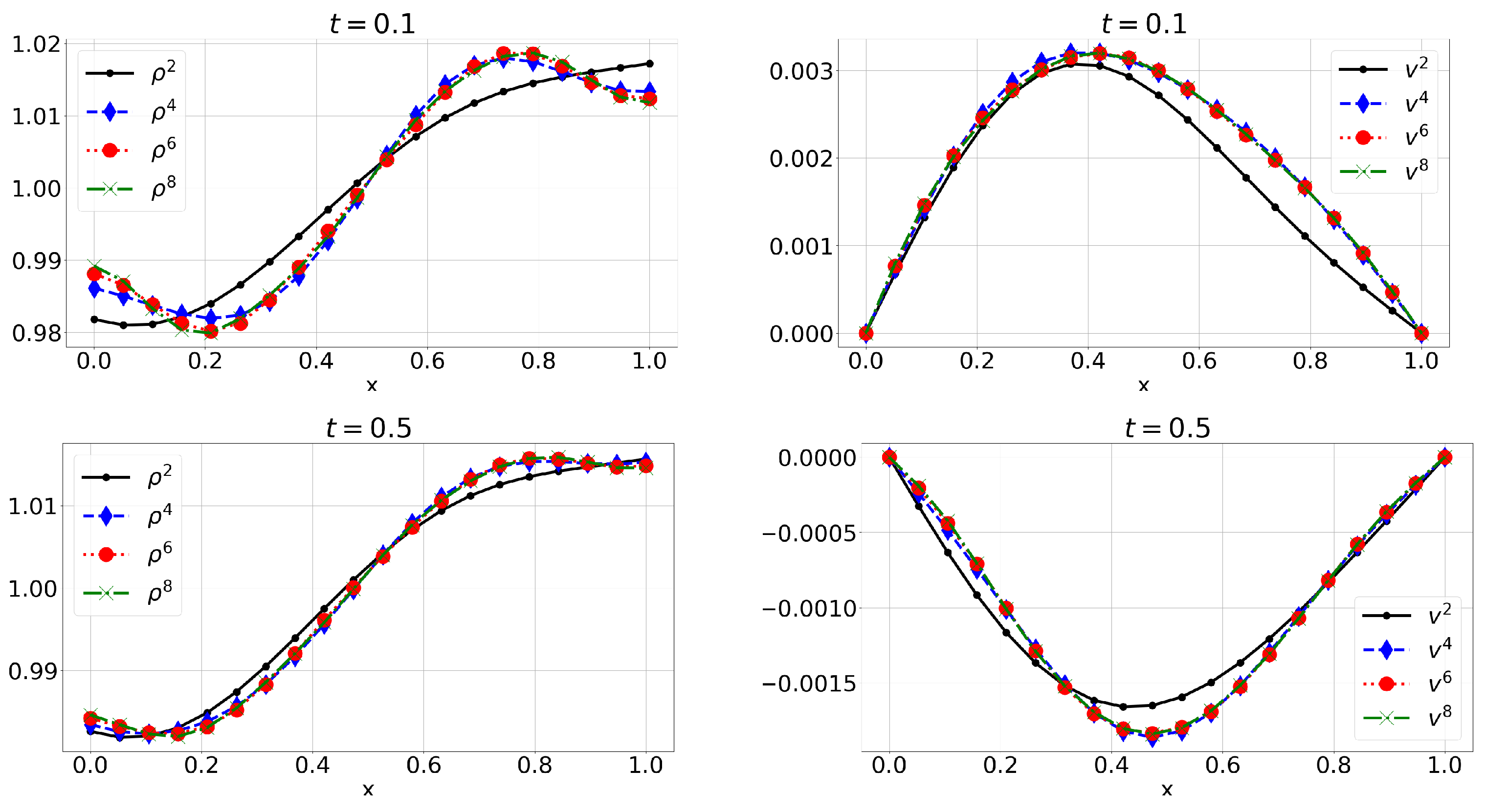
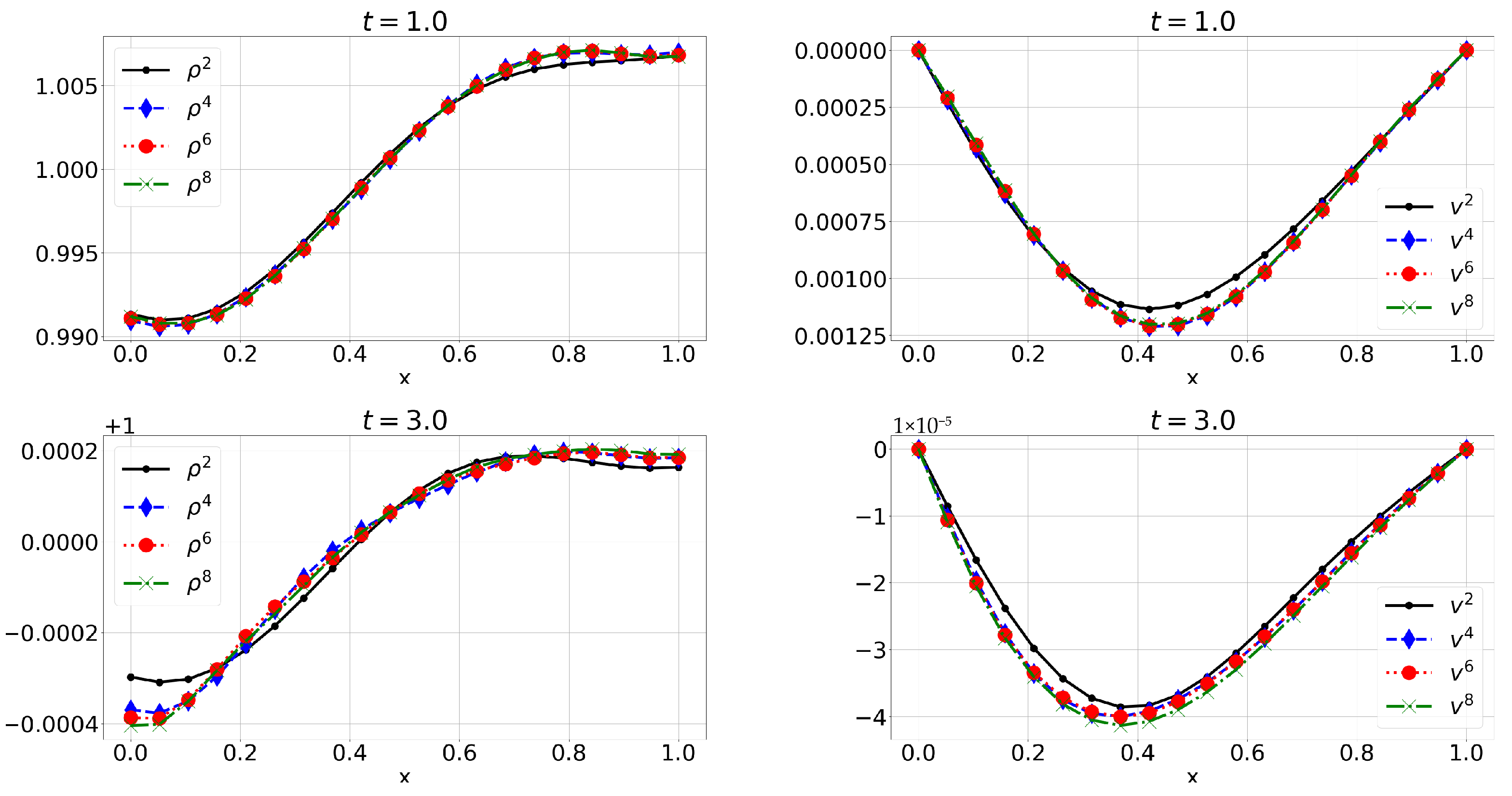
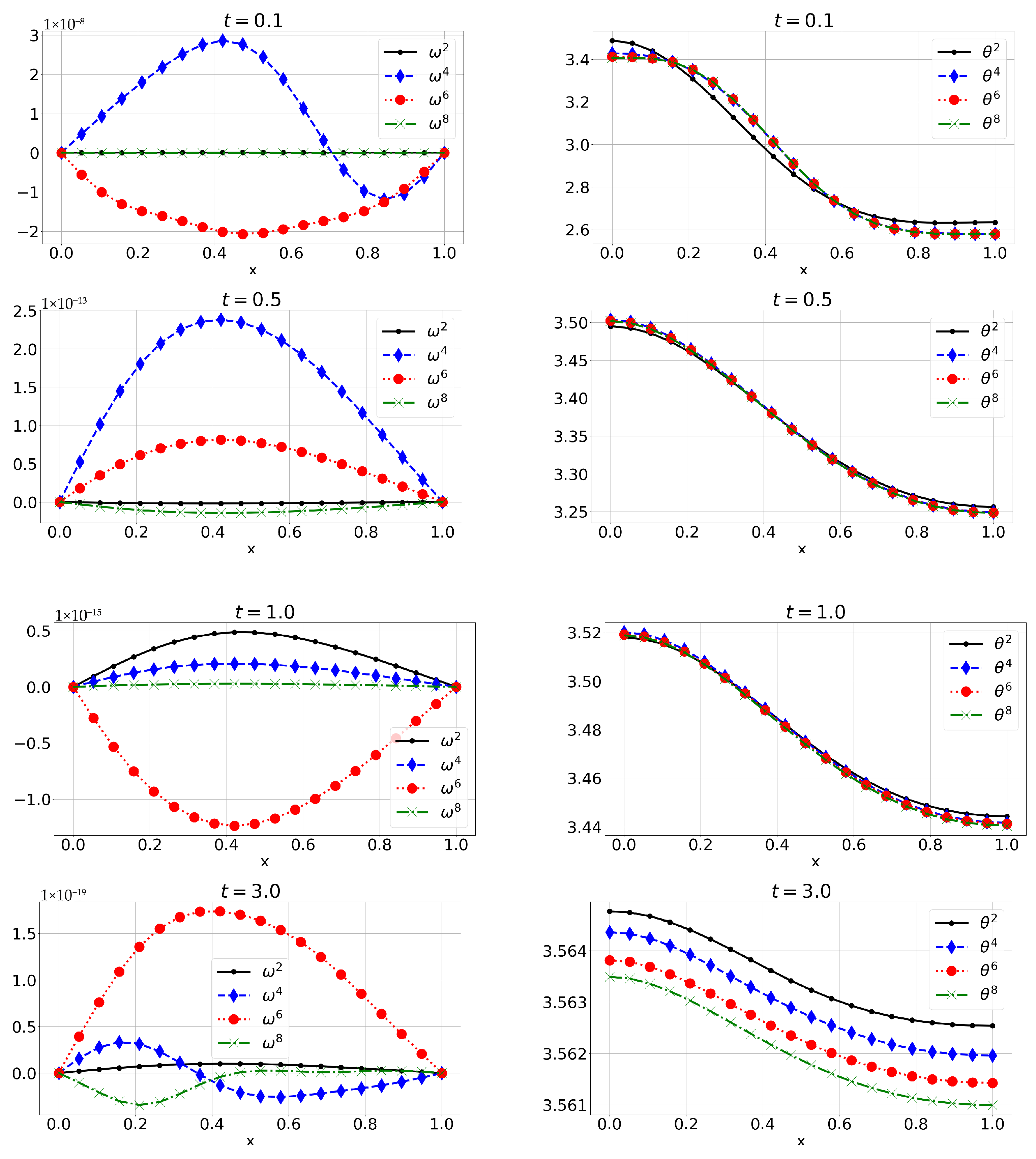
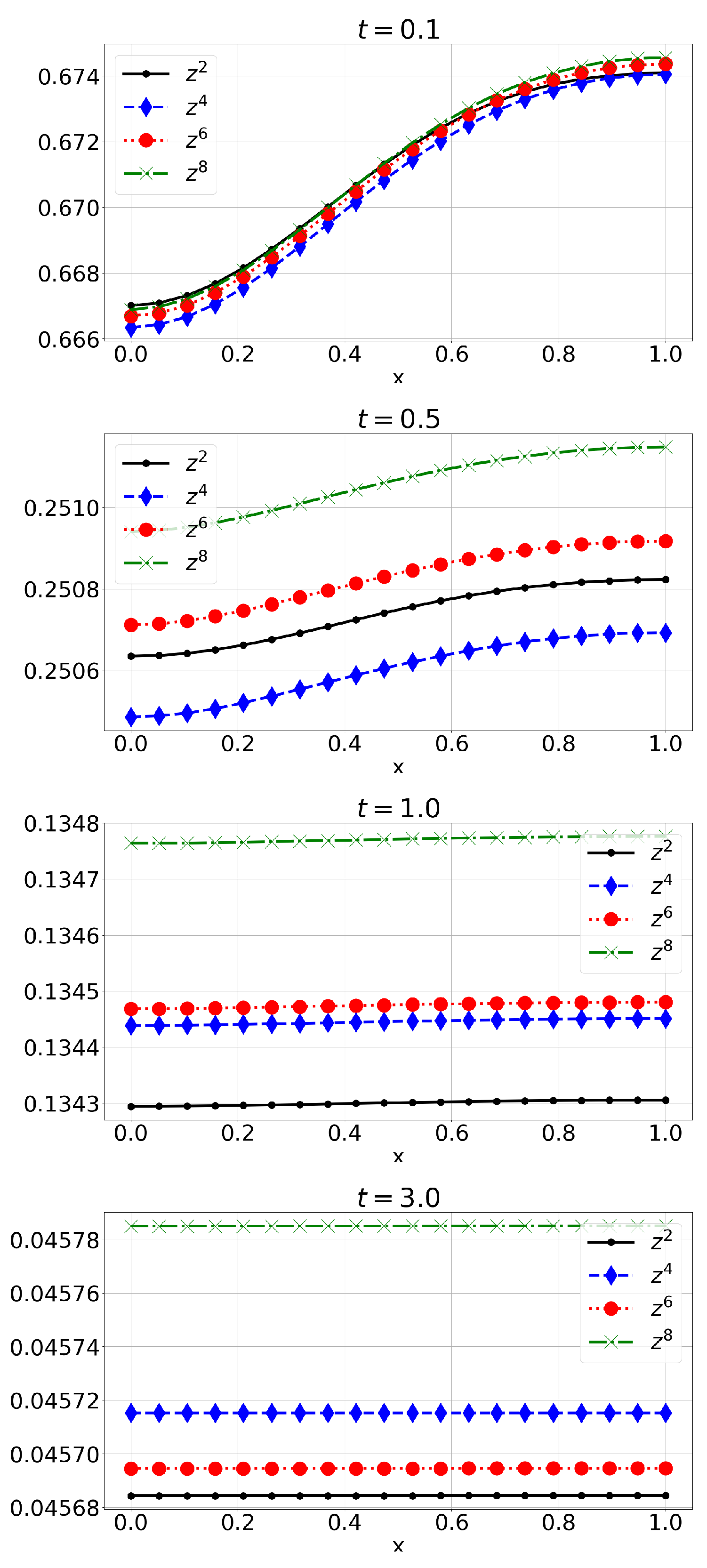
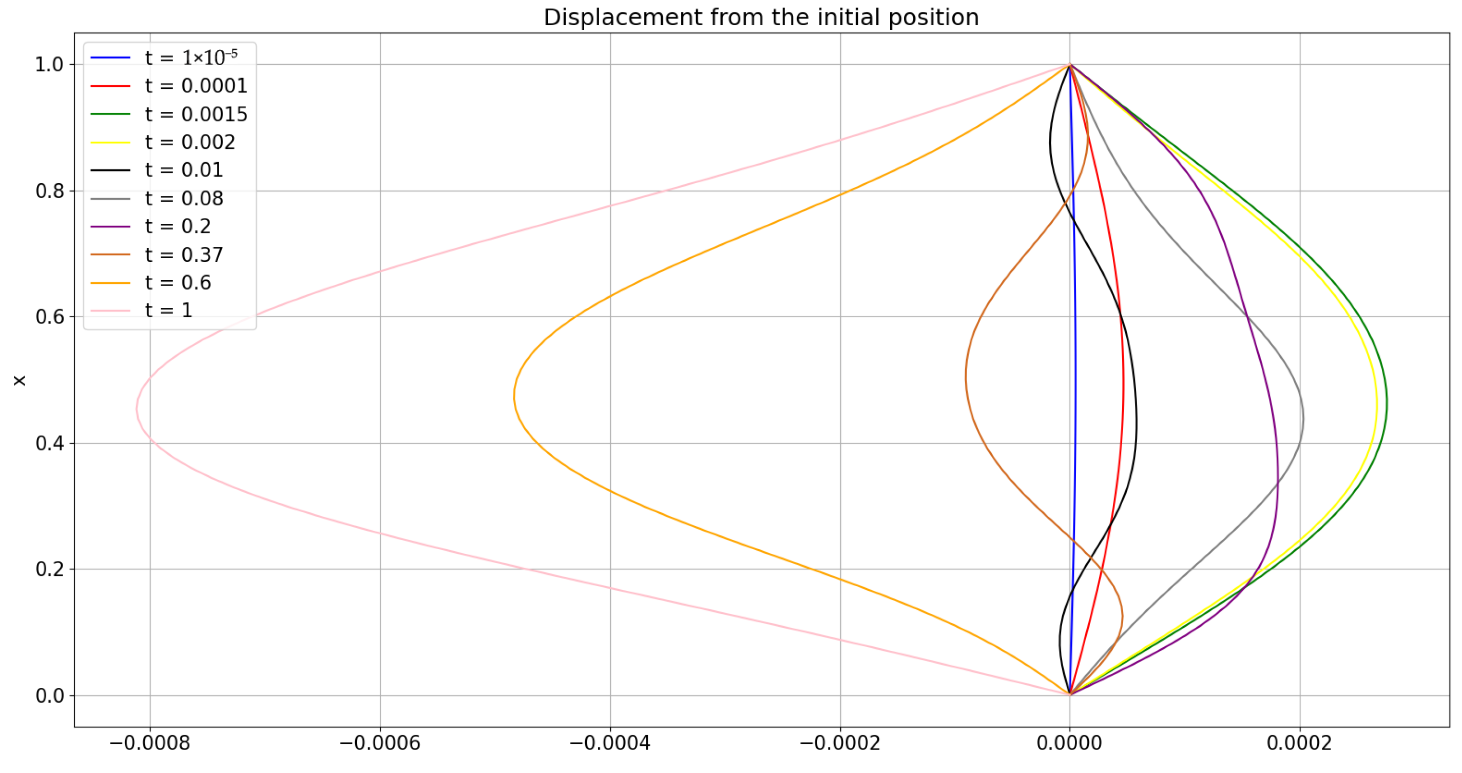
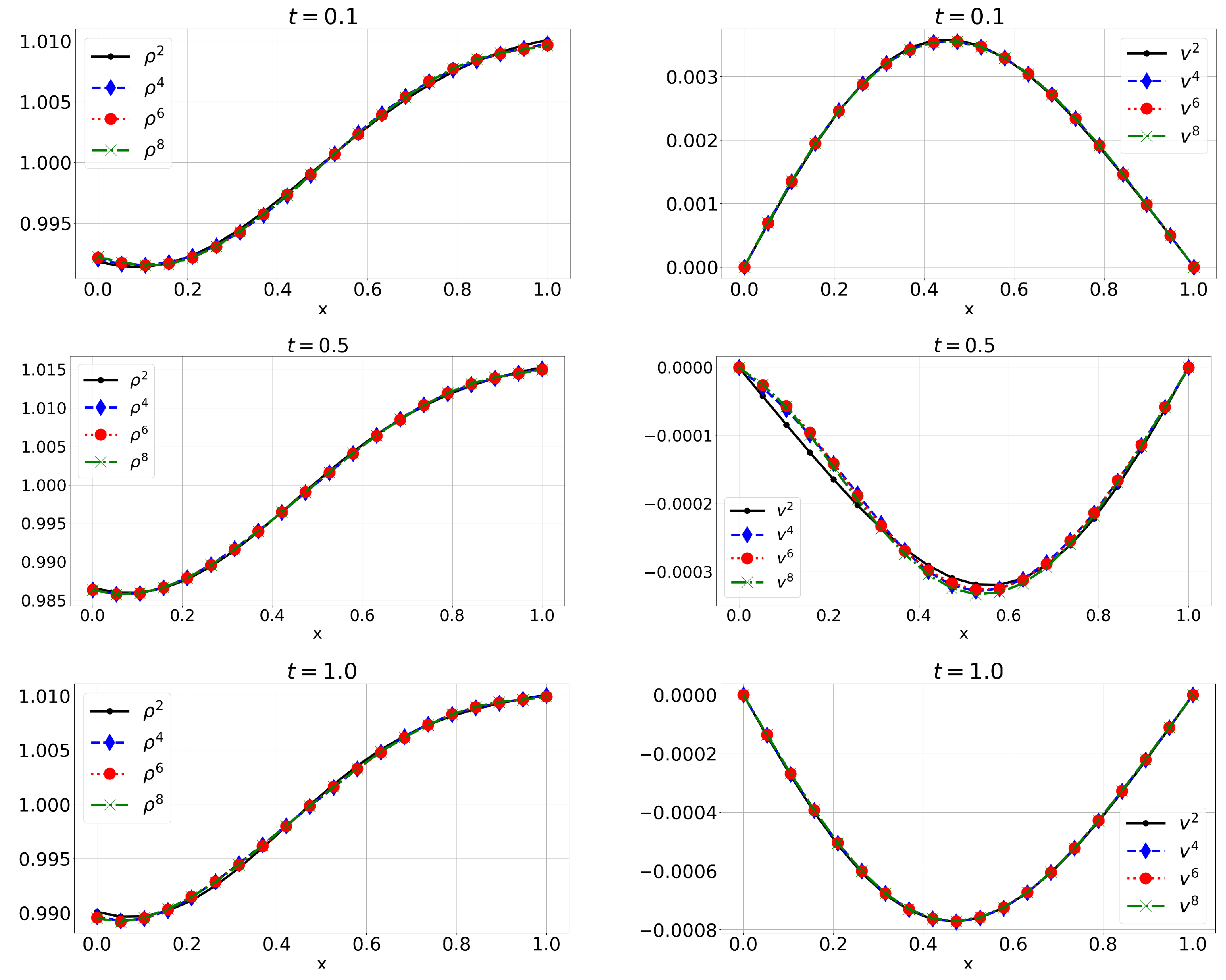
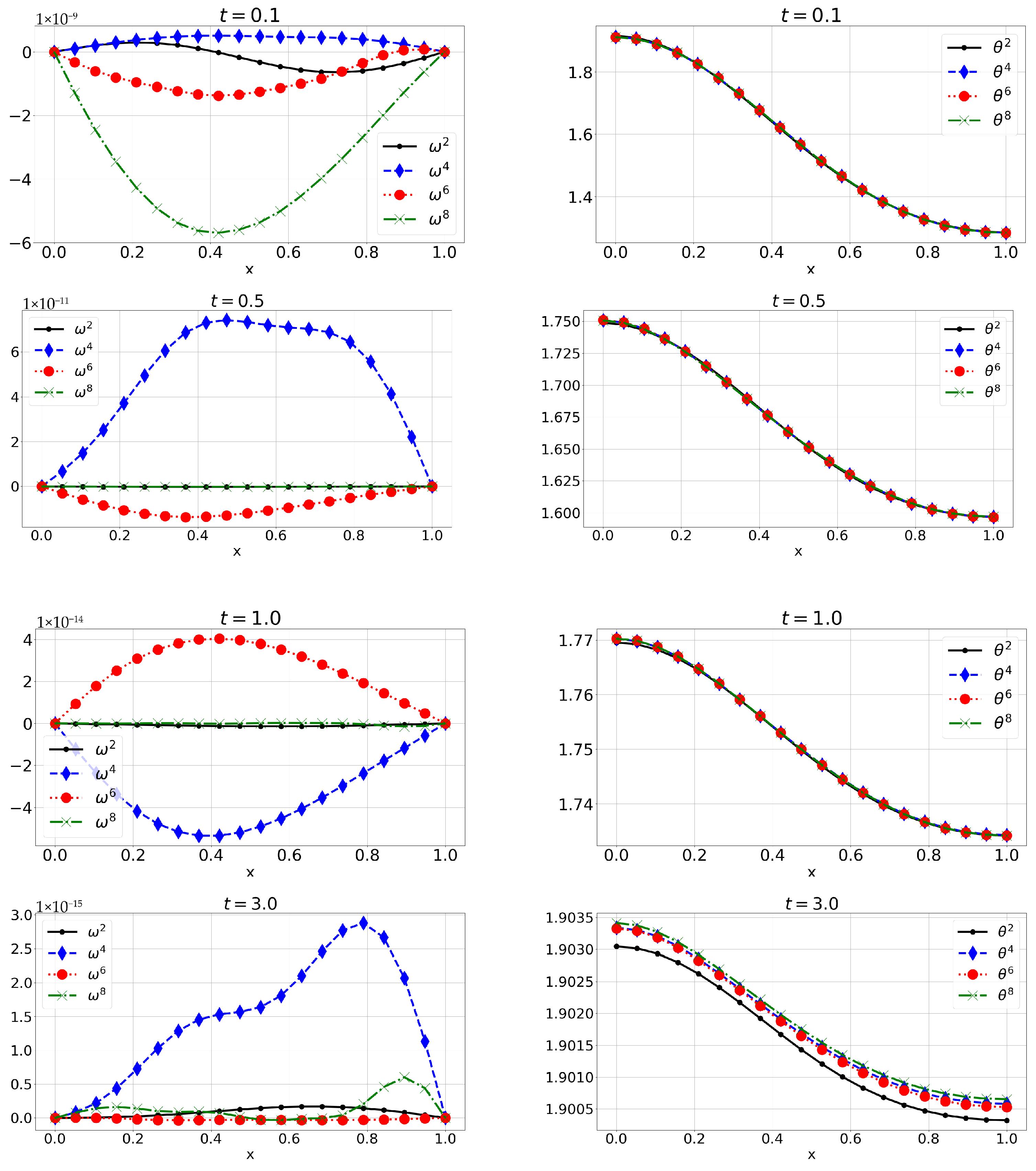
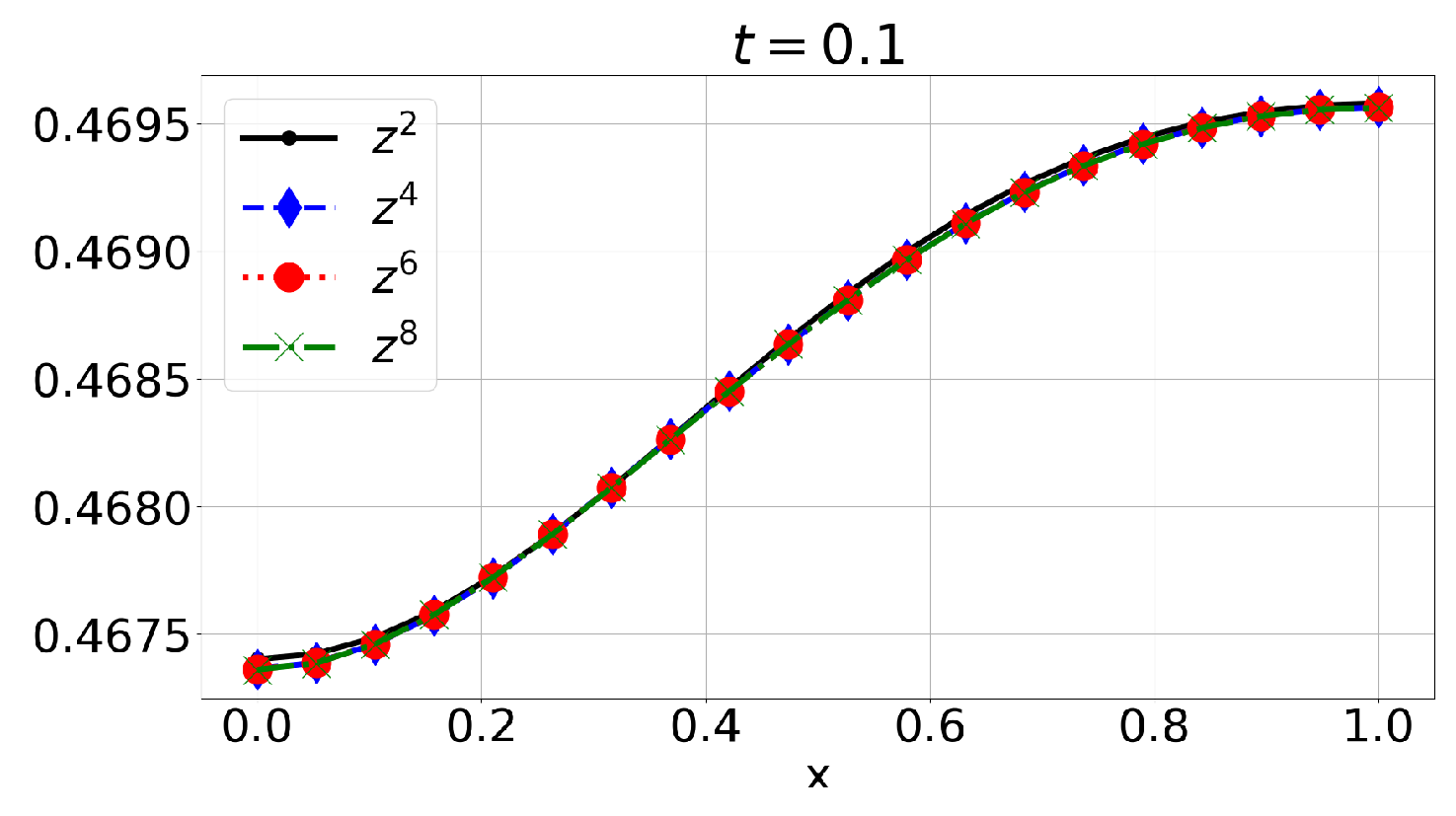
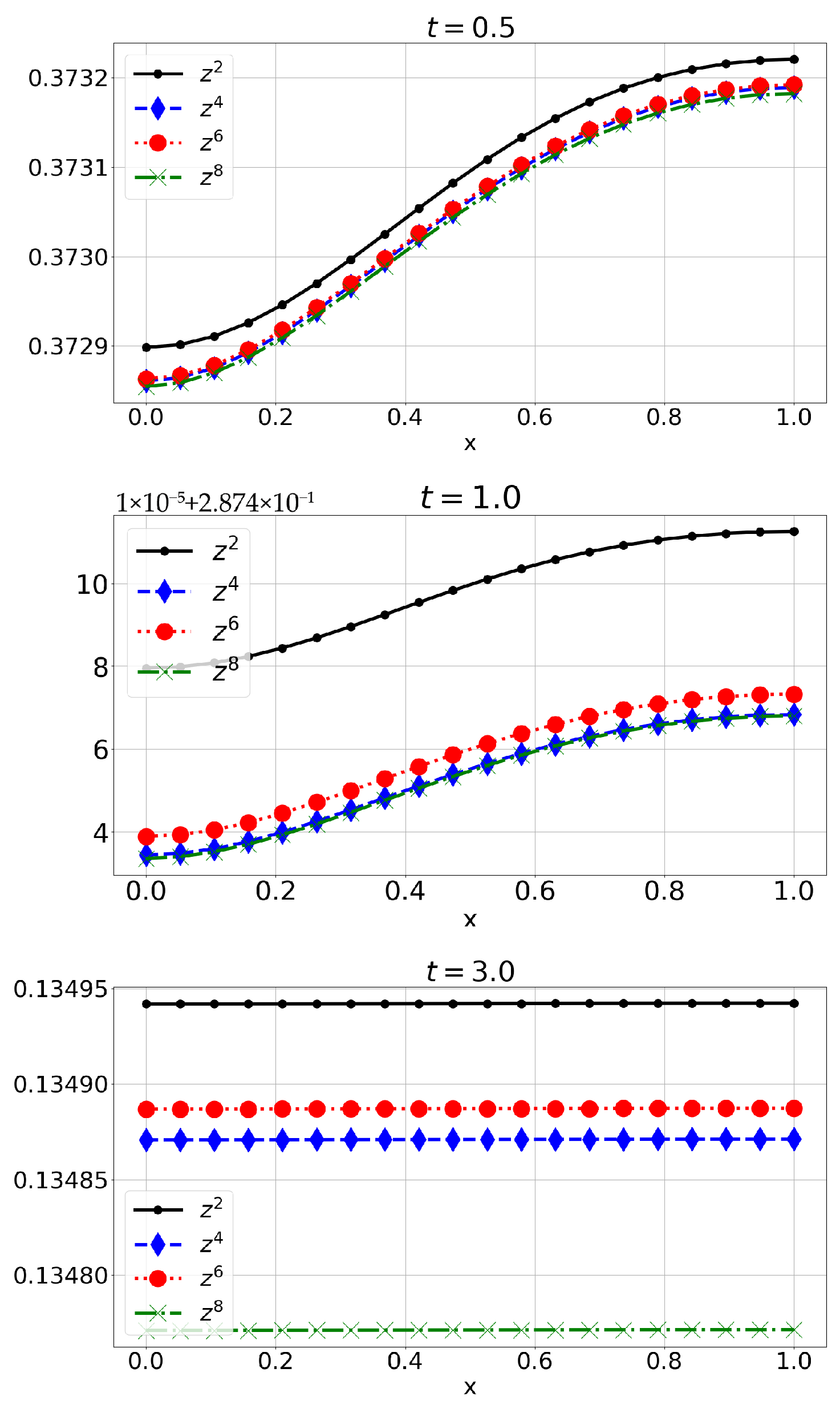
6. Numerical Solution

The approximate scheme described in Section 4 can be used to calculate a numerical solution to the initial-boundary value problem (16)–(30). Here we present the numerical experiment conducted using that scheme. Note that the initial data and parameters are artificially generated, not physical, and are used purely to test the proposed numerical method.

This approach is inspired by [12,42,43]. For the ideal non-reactive spherically symmetric micropolar model, finite differences were also used to obtain a numerical solution [6].

The method is implemented in Python 3.11 using the ODE solver based on the backward differentiation formula (BDF) method available in the SciPy library. To evaluate the system’s right-hand side numerically, we employed the Gauss–Legendre quadrature formula of order 20. The choice of methods is based on the fact that they have produced good results for similar models (see, e.g., [27,43]).

Let us set the system parameters [8,12],

$$\begin{array}{c}\hfill a=1,b=1.25\Rightarrow L={\displaystyle \frac{b^3-a^3}{3}}=0.317708\dot{3}\\ \hfill c_d=c_0=c_v=1,R=1,j_I=1,\lambda =-2,{\mu }_r=1,\mu =3,\kappa =0.024,\\ \hfill p=4,\sigma =1,\delta =1,ϵ=0.2,m=2,a=1.\end{array}$$

6.1. Example 1: Initial Conditions with Finite Fourier Expansion (E1)

Initial conditions, inspired by [3,43], are chosen as

$$\begin{array}{c}\hfill {\rho }_0\left(x\right)=1,v_0\left(x\right)=sin\left(\pi x\right),{\omega }_0\left(x\right)=sin\left(2\pi x\right),{\theta }_0\left(x\right)=2+cos\left(\pi x\right),z_0\left(x\right)=1.\end{array}$$

These initial functions are relatively simple, possessing a finite number of nontrivial Fourier coefficients.

Figure 1, Figure 2 and Figure 3 show numerical approximations ${\rho }^n$, $v^n$, ${\omega }^n$, ${\theta }^n$, and $z^n$ for mass density, velocity, microrotation, absolute temperature, and the mass fraction of unburned fuel, respectively, for $n=2,4,6,8$ at times $t=0.1,0.5,1,3$. The results show that mass density, absolute temperature, and the mass fraction remain non-negative over time, with the fuel proportion decreasing progressively. This behavior is consistent with the model’s physical interpretation. It is also evident that both velocity and microrotation decay relatively rapidly to zero. This last observation aligns with results from [16,19], where the long-term behavior of solutions for a spherically symmetric ideal micropolar gas and a one-dimensional reactive real micropolar gas was analyzed. Specifically, we expect similar asymptotic behavior in this model, namely that for larger times, v, $\omega$, and z decay to zero, while $\rho$ and $\theta$ stabilize around constant values. This behavior is clearly visible in the present example, providing experimental confirmation of the validity of both the model and the numerical scheme. However, a rigorous proof of these properties for the current model remains open, and we plan to address this in future work. It should also be noted that for increasing yet even relatively small values of n, the approximations are already quite close, which indicates that the method converges to a solution quickly. This is consistent with Theorem 1, which analytically established that the semi-discretized scheme is convergent (at least on a subsequence). The rapid convergence can be attributed to the simple initial conditions, which have a finite Fourier expansion; consequently, the approximations of the initial data are exact. The largest deviations are observed for $\omega$ in Figure 2, but these can be attributed to rounding errors due to a very small scale on the order of $\mathcal{O}\left({10}^{-13}\right)$ or smaller.

Figure 4 shows the approximation of pressure $P=R{\rho }^p\theta$, and Figure 5 shows the displacement from the initial position of the observed particles.

6.2. Example 2: Initial Conditions Are Polynomials (E2)

Initial conditions, inspired by [12,44], are chosen as

$$\begin{array}{cc}\hfill {\rho }_0\left(x\right)& =1,v_0\left(x\right)=x-x^2,{\omega }_0\left(x\right)=x^2(1-x^2),\hfill \\ \hfill & {\theta }_0\left(x\right)=2x^3-3x^2+2z_0\left(x\right)=2x^3-3x^2+1.\hfill \end{array}$$

Figure 6, Figure 7 and Figure 8 again show numerical approximations ${\rho }^n$, $v^n$, ${\omega }^n$, ${\theta }^n$, and $z^n$ for mass density, velocity, microrotation, absolute temperature, and the mass fraction of unburned fuel, respectively, for $n=2,4,6,8$ at times $t=0.1,0.5,1,3$. In this example, we observe similar behavior as in the first example (E1), which further validates the model.

7. Conclusions

In this paper, we derived a governing initial-boundary value system for the spherically symmetric model describing the flow and thermal explosion of a real micropolar reactive gas. We also developed an approximation scheme based on Faedo–Galerkin approximations, which serves a twofold purpose. First, it is used to prove the local existence of a generalized solution to the problem. Second, it provides a framework for computing numerical solutions.

We conducted numerical experiments to verify that the approximation method aligns with the physical interpretation of the model and with analytically proven properties. The results demonstrate consistency with expected behavior, supporting the validity of the proposed numerical scheme.

For future work, we plan to establish the global existence and uniqueness of the generalized solution for this model, as well as long term behavior, specifically stabilization towards a stationary solution. Additionally, we aim to develop a more efficient numerical scheme based on finite difference methods, where the current study can serve as a benchmark.

References

1. Lewicka, M.; Mucha, P. On temporal asymptotics for the pth power viscous reactive gas. Nonlinear Anal. Theory Methods Appl. 2004, 57, 951–969. [Google Scholar] [CrossRef]
2. Qin, Y.; Huang, L. Global Existence and Exponential Stability for the pth Power Viscous Reactive Gas. Nonlinear Anal.-Theory Methods Appl. 2010, 73, 2800–2818. [Google Scholar] [CrossRef]
3. Poland, J.; Kassoy, D. The induction period of a thermal explosion in a gas between infinite parallel plates. Combust. Flame 1983, 50, 259–274. [Google Scholar] [CrossRef]
4. Jiang, S. Global spherically symmetric solutions to the equations of a viscous polytropic ideal gas in an exterior domain. Commun. Math. Phys. 1996, 178, 339–374. [Google Scholar] [CrossRef]
5. Dražić, I.; Mujaković, N. 3-D flow of a compressible viscous micropolar fluid with spherical symmetry: A local existence theorem. Bound. Value Probl. 2012, 2012, 69. [Google Scholar] [CrossRef]
6. Mujaković, N.; Črnjarić-Žic, N. Finite Difference Formulation for the Model of a Compressible Viscous and Heat-Conducting Micropolar Fluid with Spherical Symmetry. In Differential and Difference Equations with Applications: ICDDEA 2015; Pinel, S., Došlá, Z., Došlý, O., Kloeden, P., Eds.; Springer Proceedings in Mathematics & Statistics; Springer: Berlin/Heidelberg, Germany, 2016; p. 164. [Google Scholar] [CrossRef]
7. Zhang, X. Spherically symmetric strong solution of compressible flow with large data and density-dependent viscosities. J. Math. Anal. Appl. 2025, 549, 129488. [Google Scholar] [CrossRef]
8. Dražić, I.; Mujaković, N.; Črnjarić-Žic, N. Three-dimensional compressible viscous micropolar fluid with cylindrical symmetry: Derivation of the model and a numerical solution. Math. Comput. Simul. 2017, 140, 107–124. [Google Scholar] [CrossRef]
9. Eringen, C.A. Simple microfluids. Int. J. Eng. Sci. 1964, 2, 205–217. [Google Scholar] [CrossRef]
10. Mujakovic, N. One-dimensional flow of a compressible viscous micropolar fluid: A local existence theorem. Glas. Mat. 1998, 33, 71–91. [Google Scholar]
11. Feireisl, E.; Novotný, A. Large time behaviour of flows of compressible, viscous, and heat conducting fluids. Math. Methods Appl. Sci. 2006, 29, 1237–1260. [Google Scholar] [CrossRef]
12. Bašić-Šiško, A.; Dražić, I. One-dimensional model and numerical solution to the viscous and heat-conducting reactive micropolar real gas flow and thermal explosion. Iran. J. Sci. Technol. Trans. Mech. Eng. 2022, 47, 19–39. [Google Scholar] [CrossRef]
13. Bašić-Šiško, A.; Dražić, I. Local existence for viscous reactive micropolar real gas flow and thermal explosion with homogeneous boundary conditions. J. Math. Anal. Appl. 2022, 509, 125988. [Google Scholar] [CrossRef]
14. Bašić-Šiško, A.; Dražić, I. Global existence theorem of a generalized solution for a one-dimensional thermal explosion model of a compressible micropolar real gas. Math. Methods Appl. Sci. 2024, 47, 10024–10039. [Google Scholar] [CrossRef]
15. Bašić-Šiško, A.; Dražić, I. Uniqueness of a Generalized Solution for a One-Dimensional Thermal Explosion Model of a Compressible Micropolar Real Gas. Mathematics 2024, 12, 717. [Google Scholar] [CrossRef]
16. Bašić-Šiško, A. Large time existence and asymptotic stability of the generalized solution to flow and thermal explosion model of reactive real micropolar gas. Math. Methods Appl. Sci. 2024, 47, 11490–11510. [Google Scholar] [CrossRef]
17. Bašić-Šiško, A.; Dražić, I.; Simčić, L. One-dimensional model and numerical solution to the viscous and heat-conducting micropolar real gas flow with homogeneous boundary conditions. Math. Comput. Simul. 2022, 195, 71–87. [Google Scholar] [CrossRef]
18. Huang, L.; Li, C.; Yan, X.; Yang, X. Asymptotic stability of one-dimensional compressible viscous and heat-conducting p-th micropolar fluid. Differ. Integral Equ. 2025, 38, 297–326. [Google Scholar] [CrossRef]
19. Dražić, I.; Mujaković, N. 3-D flow of a compressible viscous micropolar fluid with spherical symmetry: Large time behavior of the solution. J. Math. Anal. Appl. 2015, 431, 545–568. [Google Scholar] [CrossRef]
20. Simčić, L. A shear flow problem for compressible viscous micropolar fluid: Uniqueness of a generalized solution. Math. Methods Appl. Sci. 2019, 42, 6358–6368. [Google Scholar] [CrossRef]
21. Bebernes, J.; Bressan, A. Global a priori estimates for a viscous reactive gas. Proc. R. Soc. Edinb. Sect. A Math. 1985, 101, 321–333. [Google Scholar] [CrossRef]
22. Qin, Y.; Huang, L. Regularity and exponential stability of the pth Newtonian fluid in one space dimension. Math. Model. Methods Appl. Sci.–M3AS 2010, 20, 589–610. [Google Scholar] [CrossRef]
23. Wang, T. One dimensional p-th power Newtonian fluid with temperature-dependent thermal conductivity. Commun. Pure Appl. Anal. 2016, 15, 477–494. [Google Scholar] [CrossRef]
24. Cui, H.; Yao, Z.a. Asymptotic behavior of compressible p-th power Newtonian fluid with large initial data. J. Differ. Equ. 2015, 258, 919–953. [Google Scholar] [CrossRef]
25. Watson, S.; Lewicka, M. Temporal asymptotics for the p’th power Newtonian fluid in one space dimension. Z. Angew. Math. Phys. 2003, 54, 633–651. [Google Scholar] [CrossRef]
26. Wan, L.; Wang, T. Asymptotic behavior for the one-dimensional pth power Newtonian fluid in unbounded domains. Math. Methods Appl. Sci. 2015, 39, 1020–1025. [Google Scholar] [CrossRef]
27. Bašić-Šiško, A.; Simčić, L.; Dražić, I. Three-dimensional model of a spherically symmetric compressible micropolar fluid flow with real gas equation of state. Symmetry 2024, 16, 1330. [Google Scholar] [CrossRef]
28. Zhang, M. On the Cauchy problem of three-dimensional compressible magneto-micropolar fluids with vacuum. Math. Nachrichten 2025, 298, 1449–1481. [Google Scholar] [CrossRef]
29. El-Sapa, S.; Faltas, M.S. Mobilities of two spherical particles immersed in a magneto-micropolar fluid. Phys. Fluids 2022, 34, 013104. [Google Scholar] [CrossRef]
30. Pop, I.; Groșan, T.; Revnic, C.; Roșca, A.V. Unsteady flow and heat transfer of nanofluids, hybrid nanofluids, micropolar fluids and porous media: A review. Therm. Sci. Eng. Prog. 2023, 46, 102248. [Google Scholar] [CrossRef]
31. Jalili, B.; Azar, A.A.; Jalili, P.; Ganji, D.D. Analytical approach for micropolar fluid flow in a channel with porous walls. Alex. Eng. J. 2023, 79, 196–226. [Google Scholar] [CrossRef]
32. El-Sapa, S. Cell models for micropolar fluid past a porous micropolar fluid sphere with stress jump condition. Phys. Fluids 2022, 34, 082014. [Google Scholar] [CrossRef]
33. Mekheimer, K.S.; Elnaqeeb, T.; El Kot, M.; Alghamdi, F. Simultaneous effect of magnetic field and metallic nanoparticles on a micropolar fluid through an overlapping stenotic artery: Blood flow model. Phys. Essays 2016, 29, 272–283. [Google Scholar] [CrossRef]
34. Lukaszewicz, G. Micropolar Fluids: Theory and Applications; Modeling and Simulation in Science, Engineering and Technology; Birkhäuser: Boston, MA, USA, 1999. [Google Scholar]
35. Qin, Y.; Zhang, J.; Su, X.; Cao, J. Global Existence and Exponential Stability of Spherically Symmetric Solutions to a Compressible Combustion Radiative and Reactive Gas. J. Math. Fluid Mech. 2016, 18, 415–461. [Google Scholar] [CrossRef]
36. Qin, Y.; Huang, L. Global Well-Posedness of Nonlinear Parabolic-Hyperbolic Coupled Systems, 1st ed.; Frontiers in Mathematics; Birkhäuser: Basel, Swizterland, 2012. [Google Scholar] [CrossRef]
37. Antontsev, S.N.; Kazhikhov, A.V.; Monakhov, V.N. Boundary Value Problems in Mechanics of Nonhomogeneous Fluids, Volume 22; Studies in Mathematics and its Applications; North-Holland Publishing Co.: Amsterdam, Switzerland, 1989. [Google Scholar]
38. Dražić, I.; Bašić-Šiško, A. Local existence theorem for micropolar viscous real gas flow with homogeneous boundary conditions. Math. Methods Appl. Sci. 2023, 46, 5395–5421. [Google Scholar] [CrossRef]
39. Stachurska, B. On a nonlinear integral inequality. Zesz. Nauk. Uniw. Jagiellońskiego. Pr. Mat. 1971, 15, 151–157. [Google Scholar]
40. Ladyzhenskaya, O.A.; Solonnikov, V.A.; Ural’tseva, N.N. Linear and Quasilinear Equations of Parabolic Type; Translations of Mathematical Monographs; American Mathematical Society: Providence, RI, USA, 1968. [Google Scholar]
41. Evans, L. Partial Differential Equations; Graduate Studies in Mathematics; American Mathematical Society: Providence, RI, USA, 2010. [Google Scholar]
42. Dražić, I.; Mujaković, N. Approximate solution for 1-D compressible viscous micropolar fluid model in dependence of initial conditions. Int. J. Pure Appl. Math. 2008, 42, 535–540. [Google Scholar]
43. Mujaković, N.; Dražić, I. Numerical approximations of the solution for one-dimensional compressible viscous micropolar fluid model. Int. J. Pure Appl. Math. 2007, 38, 285–296. [Google Scholar]
44. Črnjarić Žic, N.; Mujaković, N. Numerical analysis of the solutions for 1d compressible viscous micropolar fluid flow with different boundary conditions. Math. Comput. Simul. 2016, 126, 45–62. [Google Scholar] [CrossRef]
Figure 1. E1: Numerical approximations of mass density ρ and velocity v for n = 2 , 4 , 6 , 8 .
Mathematics 13 02448 g001aMathematics 13 02448 g001b
Figure 2. E1: Numerical approximations of microrotation ω and temperature θ for n = 2 , 4 , 6 , 8 .
Mathematics 13 02448 g002
Figure 3. E1: Numerical approximations of the mass fraction of unburned fuel z for n = 2 , 4 , 6 , 8 .
Mathematics 13 02448 g003
Figure 4. Numerical approximations of pressure P = R ρ p θ ( n = 6 ) .
Mathematics 13 02448 g004
Figure 5. Numerical approximations of the displacement of the particles from the initial position ( n = 6 ) .
Mathematics 13 02448 g005
Figure 6. E2: Numerical approximations of mass density ρ and velocity v for n = 2 , 4 , 6 , 8 .
Mathematics 13 02448 g006aMathematics 13 02448 g006b
Figure 7. E2: Numerical approximations of microrotation ω and temperature θ for n = 2 , 4 , 6 , 8 .
Mathematics 13 02448 g007
Figure 8. E2: Numerical approximations of the mass fraction of unburned fuel z for n = 2 , 4 , 6 , 8 .
Mathematics 13 02448 g008aMathematics 13 02448 g008b
Disclaimer/Publisher’s Note: The statements, opinions and data contained in all publications are solely those of the individual author(s) and contributor(s) and not of MDPI and/or the editor(s). MDPI and/or the editor(s) disclaim responsibility for any injury to people or property resulting from any ideas, methods, instructions or products referred to in the content.