On the Convergence of the Yosida–Cayley Variational Inclusion Problem with the XOR Operation and Inertial Extrapolation Scheme

Abstract

This article studies the structure and properties of real-ordered Hilbert spaces, highlighting the roles of the XOR and XNOR logical operators in conjunction with the Yosida and Cayley approximation operators. These fundamental elements are utilized to formulate the Yosida–Cayley Variational Inclusion Problem (YCVIP) and its associated Yosida–Cayley Resolvent Equation Problem (YCREP). To address these problems, we develop and examine several solution methods, with particular attention given to the convergence behavior of the proposed algorithms. We prove both the existence of solutions and the strong convergence of iterative sequences generated under the influence of the aforesaid operators. The theoretical results are supported by a numerical result, demonstrating the practical applicability and efficiency of the suggested approaches.

1. Introduction

Variational inequality problems originate from the study of functionals constrained to convex sets and were formally introduced by Stampacchia in 1966 [1]. In his foundational work, Stampacchia developed the concept of variational inequalities to address problems involving inequalities and used the Lax–Milgram theorem [2] to investigate the regularity of solutions to partial differential equations. Since then, variational inequalities have found extensive applications in various fields, such as artificial intelligence and data science, optimal control, mechanics, finance, transportation equilibrium, and engineering sciences. Rockafellar presented a significant extension of this concept in 1976 [3], which introduced the variational inclusion problem—a broader framework that encompasses variational inequalities. In recent decades, variational inequalities and their generalizations have been actively studied in multiple mathematical settings by numerous researchers [4,5,6,7,8,9,10,11]. Hassouni and Moudafi [12] examined a class of combined variational inequalities involving single-valued mappings, later termed variational inclusions. A typical variational inclusion seeks a point at which a maximal monotone operator maps to zero. These problems serve as a unifying framework that generalizes concepts from variational inequalities, equilibrium and optimization problems, complementarity systems, mechanical models, and Nash-type equilibrium formulations.

In parallel with the development of variational theories, logical operations such as exclusive OR (XOR) and exclusive NOR (XNOR) play an essential role in digital computation. The XOR operation returns true if the two Boolean inputs differ, while XNOR yields true when the inputs are equal. These binary operations are fundamental in fault-tolerant systems, parity checking, cryptographic algorithms, and pseudorandom number generation. Both XOR and XNOR are associative and commutative and are instrumental in applications involving linear separability and logic design [13,14,15,16,17,18].

To solve non-linear operator equations and variational problems in Hilbert spaces, various approximation operators have been employed, including the resolvent, Cayley, and Yosida operators. These operators are particularly effective in approximating derivatives of convex functionals and are widely used in the study of diffusion, wave propagation, and heat transfer problems. The development of iterative algorithms based on generalized resolvent operators has been an active area of research [19], with particular attention given to improving the convergence rates of such algorithms. An important acceleration technique involves the use of inertial methods. Initially proposed by Polyak in 1964 [20] for the heavy-ball method, the inertial approach generates each new iteration using a linear combination of the two preceding terms. Chang et al. [21] applied an inertial forward–backward splitting technique to address variational inclusion problems in Hilbert spaces. More recently, Gebrie and Bedne [22] introduced a computational algorithm based on inertial extrapolation to solve generalized split common fixed-point problems, demonstrating its wide applicability. These contributions have inspired further advances in the field, including the development of new algorithms with enhanced convergence properties. Rajpoot et al. [23] recently studied a Yosida variational inclusion problem and its corresponding Yosida-resolvent equation. They employed an inertial extrapolation scheme and provided supporting numerical examples to validate their theoretical results.

Motivated by these recent advances, the present study revisits the Yosida–Cayley solution equation and its associated variational inclusion problem. We propose a novel iterative approach based on inertial extrapolation and analyze its convergence properties within Hilbert spaces. To support our theoretical findings, we provide numerical results conducted using MATLAB 2024b. The results are illustrated through convergence graphs and estimation tables, demonstrating the efficiency of the proposed algorithms.

2. Preliminaries

Let $\breve{\mathrm{\Lambda }}$ be a real-ordered Hilbert space equipped with the norm $\left|\right|.\left|\right|$ and the inner product $⟨.,.⟩$. Denote by $\kappa (\breve{\mathrm{\Lambda }})$ the collection of compact non-empty subsets of $\breve{\mathrm{\Lambda }}$, and let $\kappa \subseteq \breve{\mathrm{\Lambda }}$ be a closed convex cone. Furthermore, let $2^{\breve{\mathrm{\Lambda }}}$ denote the non-empty set consisting of subsets of $\kappa (\breve{\mathrm{\Lambda }})$.

Definition 1

([18]). Let ${\pi }_1,{\pi }_2\in \breve{\mathrm{\Lambda }},$ and let ${\kappa }_{\breve{\mathrm{\Lambda }}}$ be a cone such that $\check{\lambda }{\pi }_1\in {\kappa }_{\breve{\mathrm{\Lambda }}}.$ The cone ${\kappa }_{\breve{\mathrm{\Lambda }}}$ is said to be normal if and only if there exists a constant ${\check{\lambda }}_{{\mathrm{\Pi }}_{\breve{\mathrm{\Lambda }}}}>0$ such that

$$\parallel {\pi }_1\parallel \le {\check{\lambda }}_{{\mathrm{\Pi }}_{\breve{\mathrm{\Lambda }}}}\le \parallel {\pi }_2\parallel ,$$

where $\check{\lambda }>0$ and $0\le {\pi }_1\le {\pi }_2$.

Definition 2

([18]). A cone κ induces a partial order ≤ on $\breve{\mathrm{\Lambda }}$ defined by

$${\pi }_1\le {\pi }_2\iff {\pi }_1-{\pi }_2\in \kappa (\breve{\mathrm{\Lambda }}).$$

Two elements ${\pi }_1$ and ${\pi }_2\in \breve{\mathrm{\Lambda }},$ are said to be comparable, denoted by ${\pi }_1\propto {\pi }_2,$ if either ${\pi }_1\le {\pi }_2$ or ${\pi }_2\le {\pi }_1$.

Definition 3

([16]). Let ⊕ and ⊙ denote the XOR and XNOR operations, respectively. Consider ${\pi }_1,{\pi }_2\in \breve{\mathrm{\Lambda }}$; let ∨ and ∧ represent the operators with the least upper bound (lub) and the highest lower bound (glb), respectively. The following properties are satisfied:

 (i) 

${\pi }_1\vee {\pi }_2=inf\{{\pi }_1,{\pi }_2\}$;

 (ii) 

${\pi }_1\wedge {\pi }_2=sup\{{\pi }_1,{\pi }_2\}$;

 (iii) 

${\pi }_1\oplus {\pi }_2=({\pi }_1-{\pi }_2)\vee ({\pi }_2-{\pi }_1)$;

 (iv) 

${\pi }_1\odot {\pi }_2=({\pi }_1-{\pi }_2)\wedge ({\pi }_2-{\pi }_1)$;

 (v) 

${\pi }_1\odot {\pi }_2=0,{\pi }_1\odot {\pi }_2={\pi }_2\odot {\pi }_1,{\pi }_1\oplus {\pi }_2=0,{\pi }_1\oplus {\pi }_2={\pi }_2\oplus {\pi }_1,{\pi }_1\odot {\pi }_2=-({\pi }_1\oplus {\pi }_2);$

 (vi) 

If ${\pi }_1\propto 0$, then $-{\pi }_1\oplus 0\le {\pi }_1\oplus 0$;

 (vii) 

$(\check{\lambda }{\pi }_1)\oplus (\check{\lambda }{\pi }_2)=|\check{\lambda }|({\pi }_1\oplus {\pi }_2)$, for any scalar $\check{\lambda }$;

 (viii) 

If ${\pi }_1\propto {\pi }_2$, then $0\le {\pi }_1\oplus {\pi }_2$;

 (ix) 

If ${\pi }_1\propto {\pi }_2$, then ${\pi }_1\oplus {\pi }_2=0$ if and only if ${\pi }_1={\pi }_2$.

Proposition 1

([18]). Let ${\kappa }_{\breve{\mathrm{\Lambda }}}$ be the normal cone with normal constant ${\check{\lambda }}_{{\mathrm{\Pi }}_{\breve{\mathrm{\Lambda }}}}>0$. Then for all ${\pi }_1,{\pi }_2\in \breve{\mathrm{\Lambda }}$, the following conditions hold:

 (i) 

$\left|\right|0\oplus 0\left|\right|=\left|\right|0\left|\right|=0$;

 (ii) 

$\left|\right|{\pi }_1\vee {\pi }_2\left|\right|=\left|\right|{\pi }_1\left|\right|\vee \left|\right|{\pi }_2\left|\right|\le \left|\right|{\pi }_1\left|\right|+\left|\right|{\pi }_2\left|\right|$;

 (iii) 

$\left|\right|{\pi }_1\oplus {\pi }_2\left|\right|\le \left|\right|{\pi }_1-{\pi }_2\left|\right|\le {\check{\lambda }}_{\mathrm{\Pi }}\left|\right|{\pi }_1\oplus {\pi }_2\left|\right|$;

 (iv) 

If ${\pi }_1\propto {\pi }_2,$ then $\left|\right|{\pi }_1\oplus {\pi }_2\left|\right|\le \left|\right|{\pi }_1-{\pi }_2\left|\right|$.

Definition 4.

A mapping $p:\breve{\mathrm{\Lambda }}\to \breve{\mathrm{\Lambda }}$ is said to be Lipschitz continuous if there exists a constant ${\check{\lambda }}_p>0$ such that

$$\begin{array}{c}\hfill \left|\right|p\left({\pi }_1\right)-p\left({\pi }_2\right)\left|\right|\le {\check{\lambda }}_p\left|\right|{\pi }_1-{\pi }_2\left|\right|,\forall {\pi }_1,{\pi }_2\in \breve{\mathrm{\Lambda }}.\end{array}$$

Definition 5.

A mapping $p:\breve{\mathrm{\Lambda }}\to \breve{\mathrm{\Lambda }}$ is said to be a${\delta }_p$-ordered non-extended mapping if there exists a constant ${\delta }_p>0$ such that

$$\begin{array}{c}\hfill \left|\right|p\left({\pi }_1\right)\oplus p\left({\pi }_2\right)\left|\right|\le {\delta }_p\left|\right|{\pi }_1\oplus {\pi }_2\left|\right|,\forall {\pi }_1,{\pi }_2\in \breve{\mathrm{\Lambda }}.\end{array}$$

Definition 6.

Let $\mathrm{\Sigma }:\breve{\mathrm{\Lambda }}\times \breve{\mathrm{\Lambda }}\times \breve{\mathrm{\Lambda }}\to \breve{\mathrm{\Lambda }}$ be a single-valued mapping, and let $\Delta :\breve{\mathrm{\Lambda }}\times \breve{\mathrm{\Lambda }}\to 2^{\breve{\mathrm{\Lambda }}}$ be a multi-valued mapping. Then

 (i) 

The mapping Δ is said to be Lipschitz continuous in the first argument if there exists a constant ${\check{\lambda }}_{{\mathrm{\Sigma }}_1}>0$ such that, for any ${\mu }_1\in \Delta (.,{\pi }_1),{\mu }_2\in \Delta (.,{\pi }_2),$

$$\left|\right|\mathrm{\Sigma }({\mu }_1,.,.)-\mathrm{\Sigma }({\mu }_2,.,.)\left|\right|\le {\check{\lambda }}_{{\mathrm{\Sigma }}_1}\left|\right|{\mu }_1-{\mu }_2\left|\right|,\forall {\pi }_1,{\pi }_2\in \kappa (\breve{\mathrm{\Lambda }}).$$

 (ii) 

The mapping Δ is said to be Lipschitz continuous in the second argument if there exists a constant ${\check{\lambda }}_{{\mathrm{\Sigma }}_2}>0$ such that, for any ${\mu }_1\in \Delta (.,{\pi }_1),{\mu }_2\in \Delta (.,{\pi }_2),$

$$\left|\right|\mathrm{\Sigma }(.,{\mu }_1,.)-\mathrm{\Sigma }(.,{\mu }_2,.)\left|\right|\le {\check{\lambda }}_{{\mathrm{\Sigma }}_2}\left|\right|{\mu }_1-{\mu }_2\left|\right|,\forall {\pi }_1,{\pi }_2\in \kappa (\breve{\mathrm{\Lambda }}).$$

Definition 7.

Let $p:\breve{\mathrm{\Lambda }}\to \breve{\mathrm{\Lambda }}$ be a single-valued mapping, and let $\Delta :\breve{\mathrm{\Lambda }}\times \breve{\mathrm{\Lambda }}\to 2^{\breve{\mathrm{\Lambda }}}$ be a multi-valued mapping. Then

 (i) 

The mapping p is called a comparison mapping if for all ${\pi }_1,{\pi }_2\in \breve{\mathrm{\Lambda }}$ such that ${\pi }_1\propto {\pi }_2$, and ${\pi }_1\propto p\left({\pi }_1\right)$ and ${\pi }_2\propto p\left({\pi }_2\right)$, it holds that

$$p\left({\pi }_1\right)\propto p\left({\pi }_2\right).$$

 (ii) 

The comparison mapping Δ is said to be an α-non-ordinary difference mapping, if there exists ${\vartheta }_{{\pi }_1}\in \Delta (.,{\pi }_1)$ and ${\vartheta }_{{\pi }_2}\in \Delta (.,{\pi }_2)$ such that

$$({\vartheta }_{{\pi }_1}\oplus {\vartheta }_{{\pi }_2})\oplus \alpha ({\pi }_1\oplus {\pi }_2)=0,\forall {\pi }_1,{\pi }_2\in \breve{\mathrm{\Lambda }}.$$

 (iii) 

The comparison mapping Δ is called a ρ-ordered rectangular mapping if there exists ${\vartheta }_{{\pi }_1}\in \Delta (.,{\pi }_1)$ and ${\vartheta }_{{\pi }_2}\in \Delta (.,{\pi }_2)$ such that

$$⟨({\vartheta }_{{\pi }_1}\odot {\vartheta }_{{\pi }_2})-({\pi }_1\oplus {\pi }_2)⟩\ge \check{\lambda }\left|\right|{\pi }_1\oplus {\pi }_2{\left|\right|}^2,\forall {\pi }_1,{\pi }_2\in \breve{\mathrm{\Lambda }},\check{\lambda }>0.$$

 (iv) 

The mapping Δ is a $\check{\lambda }$-weak-ordered different mapping if there exists a constant $\check{\lambda }>0,$ and elements ${\vartheta }_{{\pi }_1}\in \Delta (·,{\pi }_1)$ and ${\vartheta }_{{\pi }_2}\in \Delta (·,{\pi }_2)$, such that

$$\check{\lambda }({\vartheta }_{{\pi }_1}-{\vartheta }_{{\pi }_2})\propto ({\pi }_1-{\pi }_2),\forall {\pi }_1,{\pi }_2\in \breve{\mathrm{\Lambda }}.$$

Definition 8.

A mapping $\breve{\psi }:\breve{\mathrm{\Lambda }}\to \kappa (\breve{\mathrm{\Lambda }})$ is said to be $\mathcal{D}$-Lipschitz continuous if there exists a constant ${\check{\lambda }}_{{\mathcal{D}}_{\psi }}>0$ such that

$$\mathcal{D}(\psi \left({\pi }_1\right),\psi \left({\pi }_2\right))\le {\check{\lambda }}_{{\mathcal{D}}_{\psi }}\left|\right|{\pi }_1-{\pi }_2\left|\right|,\forall {\pi }_1,{\pi }_2\in \kappa (\breve{\mathrm{\Lambda }}),$$

where $\mathcal{D}(.,.)$ denotes the Hausdörff metric on ${\kappa }_{\breve{\mathrm{\Lambda }}}$.

Definition 9

([19]). Let $\Delta :\breve{\mathrm{\Lambda }}\times \breve{\mathrm{\Lambda }}\to 2^{\breve{\mathrm{\Lambda }}}$ be a multi-valued mapping. The resolvent operator associated with $\Delta (.,{\pi }_1)$, denoted by ${\beta }_{(\tau ,\check{\lambda })}^{\Delta (.,\pi )}:\breve{\mathrm{\Lambda }}\to \breve{\mathrm{\Lambda }}$, is defined by for all ${\pi }_1,{\pi }_2\in \breve{\mathrm{\Lambda }}$ and $\check{\lambda }>0$ as

$$\begin{array}{c}\hfill {\beta }_{(\tau ,\check{\lambda })}^{\Delta (.,{\pi }_1)}\left({\pi }_2\right)={\left[\tau +\check{\lambda }\Delta (.,{\pi }_1)\right]}^{-1}\left({\pi }_2\right),\end{array}$$

where τ denotes the identity operator on $\breve{\mathrm{\Lambda }}$.

Definition 10.

The Yosida approximation operator $Y_{(\tau ,\check{\lambda })}^{\Delta (.,{\pi }_1)}:\breve{\mathrm{\Lambda }}\to \breve{\mathrm{\Lambda }}$ is defined as

$$\begin{array}{c}\hfill Y_{(\tau ,\check{\lambda })}^{\Delta (.,{\pi }_1)}\left({\pi }_2\right)={\displaystyle \frac{1}{\check{\lambda }}}\left[\tau -\beta (.,{\pi }_1)\right]\left({\pi }_2\right),\forall {\pi }_1,{\pi }_2\in \breve{\mathrm{\Lambda }},\check{\lambda }>0,\end{array}$$

where τ denotes the identity operator on $\breve{\mathrm{\Lambda }}$.

Definition 11.

The Cayley approximation operator associated with the multi-valued mapping $\Delta (·,{\pi }_1)$, denoted by $C_{(\tau ,\check{\lambda })}^{\Delta (·,{\pi }_1)}:\breve{\mathrm{\Lambda }}\to \breve{\mathrm{\Lambda }}$, is defined as

$$\begin{array}{c}\hfill C_{(\tau ,\check{\lambda })}^{\Delta (.,{\pi }_1)}\left({\pi }_2\right)=\left[2\beta (.,{\pi }_1)-\tau \right]\left({\pi }_2\right),\forall {\pi }_1,{\pi }_2\in \breve{\mathrm{\Lambda }},\check{\lambda }>0,\end{array}$$

where τ is the identity operator.

We need the following lemmas to prove the main results of this paper.

Lemma 1

([15]). Let $\Delta :\breve{\mathrm{\Lambda }}\times \breve{\mathrm{\Lambda }}\to 2^{\breve{\mathrm{\Lambda }}}$ be a γ-ordered rectangular multi-valued mapping with respect to the resolvent operator ${\beta }_{(\tau ,\check{\lambda })}^{\Delta (·,{\pi }_1)}$. Then, for all $\breve{l},\breve{m}\in \breve{\mathrm{\Lambda }}$, the following inequality holds:

$$\begin{array}{c}\hfill \left|\right|{\beta }_{(\tau ,\check{\lambda })}^{\Delta (.,{\pi }_1)}\left(\breve{l}\right)\oplus {\beta }_{(\tau ,\check{\lambda })}^{\Delta (.,{\pi }_1)}\left(\breve{m}\right)\left|\right|\le \theta \left|\right|\breve{l}\oplus \breve{m}\left|\right|,\end{array}$$

where $\theta ={\displaystyle \frac{1}{\gamma \check{\lambda }-1}}$, provided that $\check{\lambda }>{\displaystyle \frac{1}{\gamma }}$.

Thus, the resolvent operator ${\beta }_{(\tau ,\check{\lambda })}^{\Delta (·,{\pi }_1)}$ is Lipschitz-type continuous.

Lemma 2

([14]). Let $\Delta :\breve{\mathrm{\Lambda }}\times \breve{\mathrm{\Lambda }}\to 2^{\breve{\mathrm{\Lambda }}}$ be a $(\gamma ,\check{\lambda })$-weak-ordered rectangular different multi-valued mapping associated with the resolvent operator ${\beta }_{(\tau ,\check{\lambda })}^{\Delta (·,{\pi }_1)}$. Let $Y_{(\tau ,\check{\lambda })}^{\Delta (·,{\pi }_1)}$ be the corresponding Yosida approximation operator. Then, for all $\breve{l},\breve{m}\in \breve{\mathrm{\Lambda }}$, the following inequality holds:

$$∥Y_{(\tau ,\check{\lambda })}^{\Delta (·,{\pi }_1)}\left(\breve{l}\right)\oplus Y_{(\tau ,\check{\lambda })}^{\Delta (·,{\pi }_1)}\left(\breve{m}\right)∥\le {\theta }^{\prime }∥\breve{l}\oplus \breve{m}∥,$$

where ${\theta }^{\prime }={\displaystyle \frac{\check{\lambda }}{\gamma \check{\lambda }-1}}$, provided that $\check{\lambda }>{\displaystyle \frac{1}{\gamma }}$.

Thus, the Yosida approximation operator $Y_{(\tau ,\check{\lambda })}^{\Delta (·,{\pi }_1)}$ is Lipschitz-type continuous.

Lemma 3

([17]). Let $\Delta :\breve{\mathrm{\Lambda }}\times \breve{\mathrm{\Lambda }}\to 2^{\breve{\mathrm{\Lambda }}}$ be a $(\gamma ,\check{\lambda })$-weak-ordered rectangular different multi-valued mapping with respect to the resolvent operator ${\beta }_{(\tau ,\check{\lambda })}^{\Delta (·,{\pi }_1)}$, and let $C_{(\tau ,\check{\lambda })}^{\Delta (·,{\pi }_1)}$ denote the associated Cayley approximation operator. Then, for all $\breve{l},\breve{m}\in \breve{\mathrm{\Lambda }}$, the following inequality holds:

$$∥C_{(\tau ,\check{\lambda })}^{\Delta (·,{\pi }_1)}\left(\breve{l}\right)\oplus C_{(\tau ,\check{\lambda })}^{\Delta (·,{\pi }_1)}\left(\breve{m}\right)∥\le (2\theta +1)∥\breve{l}\oplus \breve{m}∥,$$

where $\theta ={\displaystyle \frac{1}{\gamma \check{\lambda }-1}}$, provided that $\check{\lambda }>{\displaystyle \frac{1}{\gamma }}$.

Thus, the Cayley approximation operator $C_{(\tau ,\check{\lambda })}^{\Delta (·,{\pi }_1)}$ is Lipschitz-type continuous.

3. The Yosida–Cayley Variational Inclusion Problem (YCVIP)

Let $p:\breve{\mathrm{\Lambda }}\to \breve{\mathrm{\Lambda }}$, $\Delta :\breve{\mathrm{\Lambda }}\times \breve{\mathrm{\Lambda }}\to 2^{\breve{\mathrm{\Lambda }}}$, $\mathrm{\Sigma }:\breve{\mathrm{\Lambda }}\times \breve{\mathrm{\Lambda }}\times \breve{\mathrm{\Lambda }}\to \breve{\mathrm{\Lambda }}$, and $\psi ,\varphi ,\phi :\breve{\mathrm{\Lambda }}\to \kappa (\breve{\mathrm{\Lambda }})$ be mappings. Let $Y_{(\tau ,\check{\lambda })}^{\Delta (·,\pi )}$ and $C_{(\tau ,\check{\lambda })}^{\Delta (·,\pi )}$ denote the Yosida and Cayley approximation operators associated with $\Delta (·,\pi )$, respectively. Find $\pi \in \breve{\mathrm{\Lambda }}$, $\breve{l}\in \psi \left(\pi \right)$, $\breve{m}\in \varphi \left(\pi \right)$, and $\breve{n}\in \phi \left(\pi \right)$ such that

$$\begin{array}{c}\hfill 0\in Y_{(\tau ,\check{\lambda })}^{\Delta (.,\pi )}\left(C_{(\tau ,\check{\lambda })}^{\Delta (.,\pi )}\left(\pi \right)\right)+\mathrm{\Sigma }(\breve{l},\breve{m},\breve{n})\oplus \Delta (p\left(\pi \right),\pi ),\end{array}$$

(1)

where $\check{\lambda }>0$ is a constant and $\tau$ denotes the identity mapping on $\breve{\mathrm{\Lambda }}$.

Special Case 1. 

If $Y_{(\tau ,\check{\lambda })}^{\Delta (·,\pi )}=\tau$, $\mathrm{\Sigma }(\breve{l},\breve{m},\breve{n})=0$, and $\Delta \left(p\right(\pi ),\pi )=\Delta \left(\pi \right)$, then (1) reduces to the problem of finding $\pi \in \breve{\mathrm{\Lambda }}$ such that

$$0\in C_{(\tau ,\check{\lambda })}^{\Delta (·,\pi )}\left(\pi \right)\oplus \Delta \left(\pi \right).$$

Special Case 2. 

If $Y_{(\tau ,\check{\lambda })}^{\Delta (·,\pi )}\left(C_{(\tau ,\check{\lambda })}^{\Delta (·,\pi )}\left(\pi \right)\right)=0$, $\mathrm{\Sigma }(\breve{l},\breve{m},\breve{n})=0$, and $\Delta \left(p\right(\pi ),\pi )=\Delta \left(\pi \right)$, then (1) further simplifies the classical inclusion problem of finding $\pi \in \breve{\mathrm{\Lambda }}$ such that

$$0\in \Delta \left(\pi \right).$$

This is the fundamental variational inclusion problem studied by Rockafellar [3].

4. Fixed-Point Formulation and Iterative Algorithms

Lemma 4.

The Yosida–Cayley Variational Inclusion Problem (1) admits a solution $\pi \in \breve{\mathrm{\Lambda }}$, with corresponding elements $\breve{l}\in \psi \left(\pi \right)$, $\breve{m}\in \varphi \left(\pi \right)$, and $\breve{n}\in \phi \left(\pi \right)$, if and only if the following condition is satisfied:

$$\begin{array}{c}\hfill p\left(\pi \right)={\beta }_{(\tau ,\check{\lambda })}^{\Delta (·,\pi )}\left[p\left(\pi \right)+\check{\lambda }\left\{\mathrm{\Sigma }(\breve{l},\breve{m},\breve{n})\odot Y_{(\tau ,\check{\lambda })}^{\Delta (·,\pi )}\left(C_{(\tau ,\check{\lambda })}^{\Delta (·,\pi )}\left(\pi \right)\right)\right\}\right],\end{array}$$

(2)

where $\check{\lambda }>0$, and τ denotes the identity operator.

Proof. 

Suppose $\pi \in \breve{\mathrm{\Lambda }},\breve{l}\in \psi \left(\pi \right),\breve{m}\in \varphi \left(\pi \right)$, and $\breve{n}\in \phi \left(\pi \right)$ satisfy Equation (2). Then we have,

$$\begin{array}{ccc}\hfill p\left(\pi \right)& =& {\beta }_{(\tau ,\check{\lambda })}^{\Delta (.,\pi )}\left[p\left(\pi \right)+\check{\lambda }\left\{\mathrm{\Sigma }(\breve{l},\breve{m},\breve{n})\odot Y_{(\tau ,\check{\lambda })}^{\Delta (.,\pi )}\left(C_{(\tau ,\check{\lambda })}^{\Delta (.,\pi )}\left(\pi \right)\right)\right\}\right]\hfill \\ & =& {\left[\tau +\check{\lambda }\Delta (.,\pi )\right]}^{-1}\left[p\left(\pi \right)+\check{\lambda }\left\{\mathrm{\Sigma }(\breve{l},\breve{m},\breve{n})\odot Y_{(\tau ,\check{\lambda })}^{\Delta (.,\pi )}\left(C_{(\tau ,\check{\lambda })}^{\Delta (.,\pi )}\left(\pi \right)\right)\right\}\right]\hfill \\ \hfill \left[\tau +\check{\lambda }\Delta (.,\pi )\right]p\left(\pi \right)& =& p\left(\pi \right)+\check{\lambda }\left\{\mathrm{\Sigma }(\breve{l},\breve{m},\breve{n})\odot Y_{(\tau ,\check{\lambda })}^{\Delta (.,\pi )}\left(C_{(\tau ,\check{\lambda })}^{\Delta (.,\pi )}\left(\pi \right)\right)\right\}\hfill \\ \hfill p\left(\pi \right)+\check{\lambda }\Delta (p\left(\pi \right),\pi )& =& p\left(\pi \right)+\check{\lambda }\left\{\mathrm{\Sigma }(\breve{l},\breve{m},\breve{n})\odot Y_{(\tau ,\check{\lambda })}^{\Delta (.,\pi )}\left(C_{(\tau ,\check{\lambda })}^{\Delta (.,\pi )}\left(\pi \right)\right)\right\}\hfill \\ \hfill \Delta \left(p\right(\pi ),\pi )& =& \mathrm{\Sigma }(\breve{l},\breve{m},\breve{n})\odot Y_{(\tau ,\check{\lambda })}^{\Delta (.,\pi )}\left(C_{(\tau ,\check{\lambda })}^{\Delta (.,\pi )}\left(\pi \right)\right)\hfill \\ \hfill \mathrm{\Sigma }(\breve{l},\breve{m},\breve{n})\odot \Delta (p\left(\pi \right),\pi )& =& \mathrm{\Sigma }(\breve{l},\breve{m},\breve{n})\odot \mathrm{\Sigma }(\breve{l},\breve{m},\breve{n})\odot Y_{(\tau ,\check{\lambda })}^{\Delta (.,\pi )}\left(C_{(\tau ,\check{\lambda })}^{\Delta (.,\pi )}\left(\pi \right)\right)\hfill \\ & =& Y_{(\tau ,\check{\lambda })}^{\Delta (.,\pi )}\left(C_{(\tau ,\check{\lambda })}^{\Delta (.,\pi )}\left(\pi \right)\right)\hfill \\ & 0& \in Y_{(\tau ,\check{\lambda })}^{\Delta (.,\pi )}\left(C_{(\tau ,\check{\lambda })}^{\Delta (.,\pi )}\left(\pi \right)\right)+\mathrm{\Sigma }(\breve{l},\breve{m},\breve{n})\oplus \Delta (p\left(\pi \right),\pi ).\hfill \end{array}$$

□

To solve The Yosida–Cayley Variational Inclusion Problem (YCVIP), we now develop the following method based on Lemma 4.

Algorithm 1. 

Let ${\pi }_0\in \breve{\mathrm{\Lambda }}$, and ${\breve{l}}_0\in \psi \left({\pi }_0\right)$, ${\breve{m}}_0\in \varphi \left({\pi }_0\right)$, and ${\breve{n}}_0\in \phi \left({\pi }_0\right)$ be initial elements. Define the sequences $\left\{{\pi }_n\right\}$, $\left\{{\breve{l}}_n\right\}$, $\left\{{\breve{m}}_n\right\}$, and $\left\{{\breve{n}}_n\right\}$ iteratively as follows:

$$\begin{array}{c}\hfill p\left({\pi }_{n+1}\right)={\beta }_{(\tau ,\check{\lambda })}^{\Delta (·,{\pi }_n)}\left[p\left({\pi }_n\right)+\check{\lambda }\left\{\mathrm{\Sigma }({\breve{l}}_n,{\breve{m}}_n,{\breve{n}}_n)\odot Y_{(\tau ,\check{\lambda })}^{\Delta (·,{\pi }_n)}\left(C_{(\tau ,\check{\lambda })}^{\Delta (·,{\pi }_n)}\left({\pi }_n\right)\right)\right\}\right].\end{array}$$

(3)

The above expression can equivalently be written in the symmetrized form:

$$\begin{array}{c}\hfill p\left(\pi \right)={\beta }_{(\tau ,\check{\lambda })}^{\Delta (·,\pi )}\left[{\displaystyle \frac{1}{2}}\left(p\left(\pi \right)+p\left(\pi \right)\right)+\check{\lambda }\left\{\mathrm{\Sigma }(\breve{l},\breve{m},\breve{n})\odot Y_{(\tau ,\check{\lambda })}^{\Delta (·,\pi )}\left(C_{(\tau ,\check{\lambda })}^{\Delta (·,\pi )}\left(\pi \right)\right)\right\}\right].\end{array}$$

(4)

We now propose the iterative strategy based on (4).

Algorithm 2. 

Let ${\pi }_0\in \breve{\mathrm{\Lambda }}$, ${\breve{l}}_0\in \psi \left({\pi }_0\right)$, ${\breve{m}}_0\in \varphi \left({\pi }_0\right)$, and ${\breve{n}}_0\in \phi \left({\pi }_0\right)$ be initial elements. Compute the sequences $\left\{{\pi }_n\right\}$, $\left\{{\breve{l}}_n\right\}$, $\left\{{\breve{m}}_n\right\}$, and $\left\{{\breve{n}}_n\right\}$ iteratively according to the following step-by-step procedure:

$$\begin{array}{cc}\hfill p\left({\pi }_{n+1}\right)& =(1-{\alpha }_n)p\left({\pi }_n\right)+{\alpha }_n{\beta }_{(\tau ,\check{\lambda })}^{\Delta (·,{\pi }_n)}[{\displaystyle \frac{1}{2}}\left(p\left({\pi }_n\right)+p\left({\pi }_{n+1}\right)\right)\\ & +\check{\lambda }\left\{\mathrm{\Sigma }({\breve{l}}_n,{\breve{m}}_n,{\breve{n}}_n)\odot Y_{(\tau ,\check{\lambda })}^{\Delta (·,{\pi }_n)}\left(C_{(\tau ,\check{\lambda })}^{\Delta (·,{\pi }_n)}\left({\pi }_n\right)\right)\right\}].\end{array}$$

(5)

where $n=0,1,2,\dots$ and ${\alpha }_n\in [0,1]$.

The predictor–corrector approach [24] is employed to describe the following inertial extrapolation scheme.

Algorithm 3. 

Let ${\pi }_0\in \breve{\mathrm{\Lambda }}$, with initial values ${\breve{l}}_0\in \psi \left({\pi }_0\right)$, ${\breve{m}}_0\in \varphi \left({\pi }_0\right)$, and ${\breve{n}}_0\in \phi \left({\pi }_0\right)$. Compute the sequences $\left\{{\pi }_n\right\}$, $\left\{{\breve{l}}_n\right\}$, $\left\{{\breve{m}}_n\right\}$, and $\left\{{\breve{n}}_n\right\}$ recursively as follows:

$$\begin{array}{ccc}\hfill J_n& & ={\pi }_n+e_n({\pi }_n-{\pi }_{n-1});\hfill \end{array}$$

(6)

$$\begin{array}{ccc}\hfill p\left({\pi }_{n+1}\right)& & =(1-{\alpha }_n)p\left({\pi }_n\right)+{\alpha }_n{\beta }_{(\tau ,\check{\lambda })}^{\Delta (·,{\pi }_n)}[{\displaystyle \frac{1}{2}}\left(p\left({\pi }_n\right)+p\left(J_n\right)\right)\hfill \\ & & +\check{\lambda }\left\{\mathrm{\Sigma }({\breve{l}}_n,{\breve{m}}_n,{\breve{n}}_n)\odot Y_{(\tau ,\check{\lambda })}^{\Delta (·,{\pi }_n)}\left(C_{(\tau ,\check{\lambda })}^{\Delta (·,{\pi }_n)}\left(J_n\right)\right)\right\}].\hfill \end{array}$$

(7)

where $e_n,{\alpha }_n\in [0,1]$ for all $n\ge 1$, and $e_n$ is the extrapolation coefficient.

Let ${\breve{l}}_{n+1}\in \psi \left({\pi }_{n+1}\right)$, ${\breve{m}}_{n+1}\in \varphi \left({\pi }_{n+1}\right)$, and ${\breve{n}}_{n+1}\in \phi \left({\pi }_{n+1}\right)$ be such that:

$$\begin{array}{cc}\hfill \parallel {\breve{l}}_n-{\breve{l}}_{n+1}\parallel & \le \mathcal{D}\left(\psi \left({\pi }_n\right),\psi \left({\pi }_{n-1}\right)\right);\end{array}$$

(8)

$$\begin{array}{cc}\hfill \parallel {\breve{m}}_n-{\breve{m}}_{n+1}\parallel & \le \mathcal{D}\left(\varphi \left({\pi }_n\right),\varphi \left({\pi }_{n-1}\right)\right);\end{array}$$

(9)

$$\begin{array}{cc}\hfill \parallel {\breve{n}}_n-{\breve{n}}_{n+1}\parallel & \le \mathcal{D}\left(\phi \left({\pi }_n\right),\phi \left({\pi }_{n-1}\right)\right),\end{array}$$

(10)

where $\mathcal{D}(·,·)$ denotes the Hausdorff metric on $\kappa (\breve{\mathrm{\Lambda }})$, and $\check{\lambda }>0$ is a constant.

5. Main Result

In this section, we establish the existence and strong convergence of solutions to the Yosida–Cayley Variational Inclusion Problem (YCVIP), utilizing the XOR and XNOR operations.

Theorem 1.

Suppose that $\breve{\mathrm{\Lambda }}$ is a real-ordered Hilbert space and κ is a cone that induces a partial order. Let $\mathrm{\Sigma }:\breve{\mathrm{\Lambda }}\times \breve{\mathrm{\Lambda }}\times \breve{\mathrm{\Lambda }}\to \breve{\mathrm{\Lambda }}$ be a single-valued mapping, and let $\psi ,\varphi ,\phi :\breve{\mathrm{\Lambda }}\to \kappa (\breve{\mathrm{\Lambda }})$ be multi-valued mappings. Assume that $\Delta :\breve{\mathrm{\Lambda }}\times \breve{\mathrm{\Lambda }}\to 2^{\breve{\mathrm{\Lambda }}}$ is a multi-valued mapping such that $\Delta (·,\pi )$ is a γ-ordered and $(\gamma ,\check{\lambda })$-weak-ordered rectangular different mapping with respect to its first argument. Additionally, let $p:\breve{\mathrm{\Lambda }}\to \breve{\mathrm{\Lambda }}$ be a single-valued mapping that is Lipschitz continuous with constant ${\check{\lambda }}_p$ and ${\delta }_p$-non-extended-ordered. Assume that for all $n=0,1,2,\dots$, we have ${\pi }_{n+1}\propto {\pi }_n$ and $p\left({\pi }_{n+1}\right)\propto p\left({\pi }_n\right)$. Suppose that the following conditions hold:

$$\begin{array}{cc}\hfill ∥{\beta }_{(\tau ,\check{\lambda })}^{\Delta (·,{\pi }_n)}\left(\breve{l}\right)\oplus {\beta }_{(\tau ,\check{\lambda })}^{\Delta (·,{\pi }_{n+1})}\left(\breve{l}\right)∥& \le \mu ∥{\pi }_n\oplus {\pi }_{n+1}∥;\end{array}$$

(11)

$$\begin{array}{cc}\hfill ∥Y_{(\tau ,\check{\lambda })}^{\Delta (·,{\pi }_n)}\left(\breve{l}\right)\oplus Y_{(\tau ,\check{\lambda })}^{\Delta (·,{\pi }_{n+1})}\left(\breve{l}\right)∥& \le {\mu }^{\prime }∥{\pi }_n\oplus {\pi }_{n+1}∥;\end{array}$$

(12)

$$\begin{array}{cc}\hfill ∥C_{(\tau ,\check{\lambda })}^{\Delta (·,{\pi }_n)}\left(\breve{l}\right)\oplus C_{(\tau ,\check{\lambda })}^{\Delta (·,{\pi }_{n+1})}\left(\breve{l}\right)∥& \le {\mu }^{″}∥{\pi }_n\oplus {\pi }_{n+1}∥.\end{array}$$

(13)

Further, suppose that the following inequality is satisfied:

$$\begin{array}{cc}& 0<{\displaystyle \frac{{\check{\lambda }}_{{\mathrm{\Pi }}_{\breve{\mathrm{\Lambda }}}}}{{\delta }_p}}\{(1-{\alpha }_n){\check{\lambda }}_p+{\alpha }_n\mu +{\displaystyle \frac{3}{2}}{\alpha }_n\theta {\check{\lambda }}_p+{\alpha }_n\theta \check{\lambda }({\mu }^{\prime }+{\theta }^{\prime }{\mu }^{″})+2{\alpha }_n\theta \check{\lambda }{\theta }^{\prime }(2\theta +1)\\ & +{\alpha }_n\theta \check{\lambda }({\check{\lambda }}_{{\mathrm{\Sigma }}_1}{\check{\lambda }}_{{\mathcal{D}}_{\psi }}+{\check{\lambda }}_{{\mathrm{\Sigma }}_2}{\check{\lambda }}_{{\mathcal{D}}_{\varphi }}+{\check{\lambda }}_{{\mathrm{\Sigma }}_3}{\check{\lambda }}_{{\mathcal{D}}_{\phi }})\}<1\end{array}$$

(14)

where $\theta ={\displaystyle \frac{1}{\gamma \check{\lambda }-1}}$ and ${\theta }^{\prime }={\displaystyle \frac{\check{\lambda }}{\gamma \check{\lambda }-1}}$, with $\check{\lambda }>{\displaystyle \frac{1}{\gamma }}$ for all $\breve{l},\breve{m},\breve{n}\in \breve{\mathrm{\Lambda }}$.

Let $e_n,{\alpha }_n\in [0,1]$ for all $n\ge 1$, where $e_n$ is an extrapolation term satisfying

$$\sum _{n=1}^{\infty }{\alpha }_n=\infty ,\mathrm{and}\sum _{n=1}^{\infty }{e}_n∥{\pi }_n-2{\pi }_{n-1}+{\pi }_{n-2}∥<\infty .$$

Then, the sequences $\left\{{\pi }_n\right\}$, $\left\{{\breve{l}}_n\right\}$, $\left\{{\breve{m}}_n\right\}$, and $\left\{{\breve{n}}_n\right\}$ generated by Algorithm 3 strongly converge to the solution $\pi \in \breve{\mathrm{\Lambda }}$, $\breve{l}\in \psi \left(\pi \right)$, $\breve{m}\in \varphi \left(\pi \right)$, and $\breve{n}\in \phi \left(\pi \right)$ of the YCVIP.

Proof. 

We have

$$\begin{array}{ccc}\hfill 0& \le & p\left({\pi }_{n+1}\right)\oplus p\left({\pi }_n\right)\hfill \\ & =& \{(1-{\alpha }_n)p\left({\pi }_n\right)+{\alpha }_n{\beta }_{(\tau ,\check{\lambda })}^{\Delta (.,{\pi }_n)}[{\displaystyle \frac{1}{2}}\left(p\left({\pi }_n\right)+p\left(J_n\right)\right)+\check{\lambda }\{\mathrm{\Sigma }({\breve{l}}_n,{\breve{m}}_n,{\breve{n}}_n)\hfill \\ & & \odot Y_{(\tau ,\check{\lambda })}^{\Delta (.,{\pi }_n)}\left(C_{(\tau ,\check{\lambda })}^{\Delta (.,{\pi }_n)}\left(J_n\right)\right)\left\}\right]\}\oplus \{(1-{\alpha }_n)p\left({\pi }_{n-1}\right)+{\alpha }_n{\beta }_{(\tau ,\check{\lambda })}^{\Delta (.,{\pi }_{n-1})}\left[{\displaystyle \frac{1}{2}}\right(p\left({\pi }_{n-1}\right)\hfill \\ & & +p\left(J_{n-1}\right))+\check{\lambda }\left\{\mathrm{\Sigma }({\breve{l}}_{n-1},{\breve{m}}_{n-1},{\breve{n}}_{n-1})\odot Y_{(\tau ,\check{\lambda })}^{\Delta (.,{\pi }_{n-1})}\left(C_{(\tau ,\check{\lambda })}^{\Delta (.,{\pi }_{n-1})}\left(J_{n-1}\right)\right)\right\}]\}.\hfill \\ & =& (1-{\alpha }_n)\left(p\left({\pi }_n\right)\oplus p\left({\pi }_{n-1}\right)\right)+{\alpha }_n\left\{{\beta }_{(\tau ,\check{\lambda })}^{\Delta (.,{\pi }_n)}\right[{\displaystyle \frac{1}{2}}\left(p\left({\pi }_n\right)+p\left(J_n\right)\right)\hfill \\ & & +\check{\lambda }\left\{\mathrm{\Sigma }({\breve{l}}_n,{\breve{m}}_n,{\breve{n}}_n)\odot Y_{(\tau ,\check{\lambda })}^{\Delta (.,{\pi }_n)}\left(C_{(\tau ,\check{\lambda })}^{\Delta (.,{\pi }_n)}\left(J_n\right)\right)\right\}]\oplus {\beta }_{(\tau ,\check{\lambda })}^{\Delta (.,{\pi }_{n-1})}[{\displaystyle \frac{1}{2}}(p\left({\pi }_{n-1}\right)\hfill \\ & & +p\left(J_{n-1}\right))+\check{\lambda }\left\{\mathrm{\Sigma }({\breve{l}}_{n-1},{\breve{m}}_{n-1},{\breve{n}}_{n-1})\odot Y_{(\tau ,\check{\lambda })}^{\Delta (.,{\pi }_{n-1})}\left(C_{(\tau ,\check{\lambda })}^{\Delta (.,{\pi }_{n-1})}\left(J_{n-1}\right)\right)\right\}]\}.\hfill \end{array}$$

Using (iii) of Proposition 1, we get the following.

$$\begin{array}{ccc}\hfill \left|\right|p\left({\pi }_{n+1}\right)\oplus p\left({\pi }_n\right)\left|\right|& \le & (1-{\alpha }_n){\check{\lambda }}_{{\mathrm{\Pi }}_{\breve{\mathrm{\Lambda }}}}\left|\right|p\left({\pi }_n\right)\oplus p\left({\pi }_{n-1}\right)\left|\right|+{\alpha }_n{\check{\lambda }}_{{\mathrm{\Pi }}_{\breve{\mathrm{\Lambda }}}}\left|\right|{\beta }_{(\tau ,\check{\lambda })}^{\Delta (.,{\pi }_n)}\left[{\displaystyle \frac{1}{2}}\right(p\left({\pi }_n\right)\hfill \\ & & +p\left(J_n\right))+\check{\lambda }\left\{\mathrm{\Sigma }({\breve{l}}_n,{\breve{m}}_n,{\breve{n}}_n)\odot Y_{(\tau ,\check{\lambda })}^{\Delta (.,{\pi }_n)}\left(C_{(\tau ,\check{\lambda })}^{\Delta (.,{\pi }_n)}\left(J_n\right)\right)\right\}]\hfill \\ & & \oplus {\beta }_{(\tau ,\check{\lambda })}^{\Delta (.,{\pi }_{n-1})}[{\displaystyle \frac{1}{2}}\left(p\left({\pi }_{n-1}\right)+p\left(J_{n-1}\right)\right)+\check{\lambda }\{\mathrm{\Sigma }({\breve{l}}_{n-1},{\breve{m}}_{n-1},{\breve{n}}_{n-1})\hfill \\ & & \odot Y_{(\tau ,\check{\lambda })}^{\Delta (.,{\pi }_{n-1})}\left(C_{(\tau ,\check{\lambda })}^{\Delta (.{\pi }_{n-1})}\left(J_{n-1}\right)\right)\left\}\right]\left|\right|.\hfill \end{array}$$

(15)

Substituting Equations (11)–(13) into Equation (15), we obtain the following.

$$\begin{array}{ccc}\hfill \left|\right|p\left({\pi }_{n+1}\right)\oplus p\left({\pi }_n\right)\left|\right|& \le & (1-{\alpha }_n){\check{\lambda }}_{{\mathrm{\Pi }}_{\breve{\mathrm{\Lambda }}}}\left|\right|p\left({\pi }_n\right)\oplus p\left({\pi }_{n-1}\right)\left|\right|+{\alpha }_n{\check{\lambda }}_{{\mathrm{\Pi }}_{\breve{\mathrm{\Lambda }}}}\left|\right|{\beta }_{(\tau ,\check{\lambda })}^{\Delta (.,{\pi }_n)}\left[{\displaystyle \frac{1}{2}}\right(p\left({\pi }_n\right)\hfill \\ & & +p\left(J_n\right))+\check{\lambda }\left\{\mathrm{\Sigma }({\breve{l}}_n,{\breve{m}}_n,{\breve{n}}_n)\odot Y_{(\tau ,\check{\lambda })}^{\Delta (.,{\pi }_n)}\left(C_{(\tau ,\check{\lambda })}^{\Delta (.,{\pi }_n)}\left(J_n\right)\right)\right\}]\hfill \\ & & \oplus {\beta }_{(\tau ,\check{\lambda })}^{\Delta (.,{\pi }_n)}[{\displaystyle \frac{1}{2}}\left(p\left({\pi }_{n-1}\right)+p\left(J_{n-1}\right)\right)+\check{\lambda }\{\mathrm{\Sigma }({\breve{l}}_{n-1},{\breve{m}}_{n-1},{\breve{n}}_{n-1})\hfill \\ & & \odot Y_{(\tau ,\check{\lambda })}^{\Delta (.,{\pi }_{n-1})}\left(C_{(\tau ,\check{\lambda })}^{\Delta (.,{\pi }_{n-1})}\left(J_{n-1}\right)\right)\left\}\right]\oplus {\beta }_{(\tau ,\check{\lambda })}^{\Delta (.,{\pi }_n)}[{\displaystyle \frac{1}{2}}\left(p\left({\pi }_{n-1}\right)+p\left(J_{n-1}\right)\right)\hfill \\ & & +\check{\lambda }\left\{\mathrm{\Sigma }({\breve{l}}_{n-1},{\breve{m}}_{n-1},{\breve{n}}_{n-1})\odot Y_{(\tau ,\check{\lambda })}^{\Delta (.,{\pi }_{n-1})}\left(C_{(\tau ,\check{\lambda })}^{\Delta (.,{\pi }_{n-1})}\left(J_{n-1}\right)\right)\right\}]\hfill \\ & & \oplus {\beta }_{(\tau ,\check{\lambda })}^{\Delta (.,{\pi }_{n-1})}[{\displaystyle \frac{1}{2}}\left(p\left({\pi }_{n-1}\right)+p\left(J_{n-1}\right)\right)+\check{\lambda }\{\mathrm{\Sigma }({\breve{l}}_{n-1},{\breve{m}}_{n-1},{\breve{n}}_{n-1})\hfill \\ & & \odot Y_{(\tau ,\check{\lambda })}^{\Delta (.,{\pi }_{n-1})}\left(C_{(\tau ,\check{\lambda })}^{\Delta (.,{\pi }_{n-1})}\left(J_{n-1}\right)\right)\left\}\right]\left|\right|.\hfill \end{array}$$

$$\begin{array}{ccc}& \le & (1-{\alpha }_n){\check{\lambda }}_{{\mathrm{\Pi }}_{\breve{\mathrm{\Lambda }}}}\left|\right|p\left({\pi }_n\right)\oplus p\left({\pi }_{n-1}\right)\left|\right|+{\alpha }_n{\check{\lambda }}_{{\mathrm{\Pi }}_{\breve{\mathrm{\Lambda }}}}\left|\right|{\beta }_{(\tau ,\check{\lambda })}^{\Delta (.,{\pi }_n)}\left[{\displaystyle \frac{1}{2}}\right(p\left({\pi }_n\right)\hfill \\ & & +p\left(J_n\right))+\check{\lambda }\left\{\mathrm{\Sigma }({\breve{l}}_n,{\breve{m}}_n,{\breve{n}}_n)\odot Y_{(\tau ,\check{\lambda })}^{\Delta (.,{\pi }_n)}\left(C_{(\tau ,\check{\lambda })}^{\Delta (.,{\pi }_n)}\left(J_n\right)\right)\right\}]\hfill \\ & & \oplus {\beta }_{(\tau ,\check{\lambda })}^{\Delta (.,{\pi }_n)}[{\displaystyle \frac{1}{2}}\left(p\left({\pi }_{n-1}\right)+p\left(J_{n-1}\right)\right)+\check{\lambda }\{\mathrm{\Sigma }({\breve{l}}_{n-1},{\breve{m}}_{n-1},{\breve{n}}_{n-1})\hfill \\ & & \odot Y_{(\tau ,\check{\lambda })}^{\Delta (.,{\pi }_{n-1})}\left(C_{(\tau ,\check{\lambda })}^{\Delta (.,{\pi }_{n-1})}\left(J_{n-1}\right)\right)\left\}\right]\left|\right|+{\alpha }_n{\check{\lambda }}_{{\mathrm{\Pi }}_{\breve{\mathrm{\Lambda }}}}\left|\right|{\beta }_{(\tau ,\check{\lambda })}^{\Delta (.,{\pi }_n)}\left[{\displaystyle \frac{1}{2}}\right(p\left({\pi }_{n-1}\right)\hfill \\ & & +p\left(J_{n-1}\right))+\check{\lambda }\{\mathrm{\Sigma }({\breve{l}}_{n-1},{\breve{m}}_{n-1},{\breve{n}}_{n-1})\odot Y_{(\tau ,\check{\lambda })}^{\Delta (.,{\pi }_{n-1})}(C_{(\tau ,\check{\lambda })}^{\Delta (.,{\pi }_{n-1})}\hfill \\ & & \left(J_{n-1}\right)\left)\right\}]\oplus {\beta }_{(\tau ,\check{\lambda })}^{\Delta (.,{\pi }_{n-1})}[{\displaystyle \frac{1}{2}}\left(p\left({\pi }_{n-1}\right)+p\left(J_{n-1}\right)\right)+\check{\lambda }\left\{\mathrm{\Sigma }\right({\breve{l}}_{n-1},\hfill \\ & & {\breve{m}}_{n-1},{\breve{n}}_{n-1})\odot Y_{(\tau ,\check{\lambda })}^{\Delta (.,{\pi }_{n-1})}\left(C_{(\tau ,\check{\lambda })}^{\Delta (.{\pi }_{n-1})}\left(J_{n-1}\right)\right)\left\}\right]\left|\right|\hfill \\ & \le & (1-{\alpha }_n){\check{\lambda }}_{{\mathrm{\Pi }}_{\breve{\mathrm{\Lambda }}}}\left|\right|p\left({\pi }_n\right)\oplus p\left({\pi }_{n-1}\right)\left|\right|+{\alpha }_n\mu {\check{\lambda }}_{{\mathrm{\Pi }}_{\breve{\mathrm{\Lambda }}}}\left|\right|{\pi }_n\oplus {\pi }_{n-1}\left|\right|\hfill \\ & & +{\alpha }_n\theta {\check{\lambda }}_{{\mathrm{\Pi }}_{\breve{\mathrm{\Lambda }}}}\left|\right|[{\displaystyle \frac{1}{2}}\left(p\left({\pi }_n\right)+p\left(J_n\right)\right)+\check{\lambda }\{\mathrm{\Sigma }({\breve{l}}_n,{\breve{m}}_n,{\breve{n}}_n)\hfill \\ & & \odot Y_{(\tau ,\check{\lambda })}^{\Delta (.,{\pi }_n)}\left(C_{(\tau ,\check{\lambda })}^{\Delta (.,{\pi }_n)}\left(J_n\right)\right)\left\}\right]\oplus [{\displaystyle \frac{1}{2}}\left(p\left({\pi }_{n-1}\right)+p\left(J_{n-1}\right)\right)\hfill \\ & & +\check{\lambda }\left\{\mathrm{\Sigma }({\breve{l}}_{n-1},{\breve{m}}_{n-1},{\breve{n}}_{n-1})\odot Y_{(\tau ,\check{\lambda })}^{\Delta (.,{\pi }_{n-1})}\left(C_{(\tau ,\check{\lambda })}^{\Delta (.,{\pi }_{n-1})}\left(J_{n-1}\right)\right)\right\}\left]\right||.\hfill \\ & \le & {\check{\lambda }}_{{\mathrm{\Pi }}_{\breve{\mathrm{\Lambda }}}}\{\left((1-{\alpha }_n)+{\displaystyle \frac{1}{2}}{\alpha }_n\theta \right)\left|\right|p\left({\pi }_n\right)\oplus p\left({\pi }_{n-1}\right)\left|\right|+{\alpha }_n\mu \left|\right|{\pi }_n\hfill \\ & & \oplus {\pi }_{n-1}\left|\right|+{\displaystyle \frac{1}{2}}{\alpha }_n\theta \left|\right|p\left(J_n\right)\oplus p\left(J_{n-1}\right)\left)\right||+{\alpha }_n\theta \check{\lambda }\left|\right|\mathrm{\Sigma }({\breve{l}}_n,{\breve{m}}_n,{\breve{n}}_n)\hfill \\ & & \oplus \mathrm{\Sigma }({\breve{l}}_{n-1},{\breve{m}}_{n-1},{\breve{n}}_{n-1})\left|\right|+{\alpha }_n\theta \check{\lambda }\left|\right|Y_{(\tau ,\check{\lambda })}^{\Delta (.,{\pi }_n)}\left(C_{(\tau ,\check{\lambda })}^{\Delta (.,{\pi }_n)}\left(J_n\right)\right)\hfill \\ & & \oplus Y_{(\tau ,\check{\lambda })}^{\Delta (.,{\pi }_{n-1})}\left(C_{(\tau ,\check{\lambda })}^{\Delta (.,{\pi }_{n-1})}\left(J_{n-1}\right)\right)\left|\right|\}.\hfill \end{array}$$

(16)

From the definition of $\mathcal{D}$-Lipschitz continuity and part (i) of Proposition 1, it follows that

$$\begin{array}{ccc}& & \left|\right|\mathrm{\Sigma }({\breve{l}}_n,{\breve{m}}_n,{\breve{n}}_n)\oplus \mathrm{\Sigma }({\breve{l}}_{n-1},{\breve{m}}_{n-1},{\breve{n}}_{n-1})\left|\right|\hfill \\ & =& \left|\right|\mathrm{\Sigma }({\breve{l}}_n,{\breve{m}}_n,{\breve{n}}_n)\oplus \mathrm{\Sigma }({\breve{l}}_{n-1},{\breve{m}}_n,{\breve{n}}_n)\oplus \mathrm{\Sigma }({\breve{l}}_{n-1},{\breve{m}}_n,{\breve{n}}_n)\hfill \\ & & \oplus \mathrm{\Sigma }({\breve{l}}_{n-1},{\breve{m}}_{n-1},{\breve{n}}_n)\oplus \mathrm{\Sigma }({\breve{l}}_{n-1},{\breve{m}}_{n-1},{\breve{n}}_n)\oplus \mathrm{\Sigma }({\breve{l}}_{n-1},{\breve{m}}_{n-1},{\breve{n}}_{n-1})\left|\right|\hfill \\ & =& \left|\right|\mathrm{\Sigma }({\breve{l}}_n,{\breve{m}}_n,{\breve{n}}_n)\oplus \mathrm{\Sigma }({\breve{l}}_{n-1},{\breve{m}}_n,{\breve{n}}_n)\left|\right|+\left|\right|\mathrm{\Sigma }({\breve{l}}_{n-1},{\breve{m}}_n,{\breve{n}}_n)\hfill \\ & & \oplus \mathrm{\Sigma }({\breve{l}}_{n-1},{\breve{m}}_{n-1},{\breve{n}}_n)\left|\right|+\left|\right|\mathrm{\Sigma }({\breve{l}}_{n-1},{\breve{m}}_{n-1},{\breve{n}}_n)\oplus \mathrm{\Sigma }({\breve{l}}_{n-1},{\breve{m}}_{n-1},{\breve{n}}_{n-1})\left|\right|\hfill \\ & \le & {\check{\lambda }}_{{\mathrm{\Sigma }}_1}\left|\right|{\breve{l}}_n\oplus {\breve{l}}_{n-1}\left|\right|+{\check{\lambda }}_{{\mathrm{\Sigma }}_2}\left|\right|{\breve{m}}_n\oplus {\breve{m}}_{n-1}\left|\right|+{\check{\lambda }}_{{\mathrm{\Sigma }}_3}\left|\right|{\breve{n}}_n\oplus {\breve{n}}_{n-1}\left|\right|\hfill \\ & \le & {\check{\lambda }}_{{\mathrm{\Sigma }}_1}\mathcal{D}(\psi \left({\pi }_n\right),\psi \left({\pi }_{n-1}\right))+{\check{\lambda }}_{{\mathrm{\Sigma }}_2}\mathcal{D}(\varphi \left({\pi }_n\right),\varphi \left({\pi }_{n-1}\right))+{\check{\lambda }}_{{\mathrm{\Sigma }}_3}\mathcal{D}(\phi \left({\pi }_n\right),\phi \left({\pi }_{n-1}\right))\hfill \\ & \le & {\check{\lambda }}_{{\mathrm{\Sigma }}_1}{\check{\lambda }}_{{\mathcal{D}}_{\psi }}\left|\right|{\pi }_n\oplus {\pi }_{n-1}\left|\right|+{\check{\lambda }}_{{\mathrm{\Sigma }}_2}{\check{\lambda }}_{{\mathcal{D}}_{\varphi }}\left|\right|{\pi }_n\oplus {\pi }_{n-1}\left|\right|+{\check{\lambda }}_{{\mathrm{\Sigma }}_3}{\check{\lambda }}_{{\mathcal{D}}_{\phi }}\left|\right|{\pi }_n\oplus {\pi }_{n-1}\left|\right|\hfill \\ & \le & \{{\check{\lambda }}_{{\mathrm{\Sigma }}_1}{\check{\lambda }}_{{\mathcal{D}}_{\psi }}+{\check{\lambda }}_{{\mathrm{\Sigma }}_2}{\check{\lambda }}_{{\mathcal{D}}_{\varphi }}+{\check{\lambda }}_{{\mathrm{\Sigma }}_3}{\check{\lambda }}_{{\mathcal{D}}_{\phi }}\}\left|\right|{\pi }_n\oplus {\pi }_{n-1}\left|\right|.\hfill \end{array}$$

(17)

Furthermore, by the Lipschitz continuity of the YCVIP operator and (i) of Proposition 1, we obtain the following.

$$\begin{array}{ccc}& & \left|\right|Y_{(\tau ,\check{\lambda })}^{\Delta (.,{\pi }_n)}\left(C_{(\tau ,\check{\lambda })}^{\Delta (.,{\pi }_n)}\left(J_n\right)\right)\oplus Y_{(\tau ,\check{\lambda })}^{\Delta (.,{\pi }_{n-1})}\left(C_{(\tau ,\check{\lambda })}^{\Delta (.,{\pi }_{n-1})}\left(J_{n-1}\right)\right)\left|\right|\hfill \\ & =& \left|\right|Y_{(\tau ,\check{\lambda })}^{\Delta (.,{\pi }_n)}\left(C_{(\tau ,\check{\lambda })}^{\Delta (.,{\pi }_n)}\left(J_n\right)\right)\oplus Y_{(\tau ,\check{\lambda })}^{\Delta (.,{\pi }_{n-1})}\left(C_{(\tau ,\check{\lambda })}^{\Delta (.,{\pi }_n)}\left(J_n\right)\right)\hfill \\ & & \oplus Y_{(\tau ,\check{\lambda })}^{\Delta (.,{\pi }_{n-1})}\left(C_{(\tau ,\check{\lambda })}^{\Delta (.,{\pi }_n)}\left(J_n\right)\right)\oplus Y_{(\tau ,\check{\lambda })}^{\Delta (.,{\pi }_{n-1})}\left(C_{(\tau ,\check{\lambda })}^{\Delta (.,{\pi }_{n-1})}\left(J_{n-1}\right)\right)\left|\right|\hfill \end{array}$$

$$\begin{array}{ccc}& \le & \left|\right|Y_{(\tau ,\check{\lambda })}^{\Delta (.,{\pi }_n)}\left(C_{(\tau ,\check{\lambda })}^{\Delta (.,{\pi }_n)}\left(J_n\right)\right)\oplus Y_{(\tau ,\check{\lambda })}^{\Delta (.,{\pi }_{n-1})}\left(C_{(\tau ,\check{\lambda })}^{\Delta (.,{\pi }_n)}\left(J_n\right)\right)\left|\right|\hfill \\ & & +\left|\right|Y_{(\tau ,\check{\lambda })}^{\Delta (.,{\pi }_{n-1})}\left(C_{(\tau ,\check{\lambda })}^{\Delta (.,{\pi }_n)}\left(J_n\right)\right)\oplus Y_{(\tau ,\check{\lambda })}^{\Delta (.,{\pi }_{n-1})}\left(C_{(\tau ,\check{\lambda })}^{\Delta (.,{\pi }_{n-1})}\left(J_{n-1}\right)\right)\left|\right|\hfill \\ & \le & {\mu }^{\prime }\left|\right|{\pi }_n\oplus {\pi }_{n-1}\left|\right|+{\theta }^{\prime }\left|\right|C_{(\tau ,\check{\lambda })}^{\Delta (.,{\pi }_n)}\left(J_n\right)\oplus C_{(\tau ,\lambda )}^{\Delta (.,{\pi }_{n-1})}\left(J_{n-1}\right)\left|\right|\hfill \\ & \le & {\mu }^{\prime }\left|\right|{\pi }_n\oplus {\pi }_{n-1}\left|\right|+{\theta }^{\prime }\left|\right|C_{(\tau ,\check{\lambda })}^{\Delta (.,{\pi }_n)}\left(J_n\right)\oplus C_{(\tau ,\check{\lambda })}^{\Delta (.,{\pi }_{n-1})}\left(J_n\right)\hfill \\ & & \oplus C_{(\tau ,\check{\lambda })}^{\Delta (.,{\pi }_{n-1})}\left(J_n\right)\oplus C_{(\tau ,\check{\lambda })}^{\Delta (.,{\pi }_{n-1})}\left(J_{n-1}\right)\left|\right|\hfill \\ & \le & {\mu }^{\prime }\left|\right|{\pi }_n\oplus {\pi }_{n-1}\left|\right|+{\theta }^{\prime }\left|\right|C_{(\tau ,\check{\lambda })}^{\Delta (.,{\pi }_n)}\left(J_n\right)\oplus C_{(\tau ,\check{\lambda })}^{\Delta (.,{\pi }_{n-1})}\left(J_n\right)\left|\right|\hfill \\ & & +{\theta }^{\prime }\left|\right|C_{(\tau ,\check{\lambda })}^{\Delta (.,{\pi }_{n-1})}\left(J_n\right)\oplus C_{(\tau ,\check{\lambda })}^{\Delta (.,{\pi }_{n-1})}\left(J_{n-1}\right)\left|\right|\hfill \\ & \le & {\mu }^{\prime }\left|\right|{\pi }_n\oplus {\pi }_{n-1}\left|\right|+{\theta }^{\prime }{\mu }^{″}\left|\right|{\pi }_n\oplus {\pi }_{n-1}\left|\right|+{\theta }^{\prime }(2\theta +1)\left|\right|J_n\oplus J_{n-1}\left|\right|\hfill \\ & \le & ({\mu }^{\prime }+{\theta }^{\prime }{\mu }^{″})\left|\right|{\pi }_n\oplus {\pi }_{n-1}\left|\right|+{\theta }^{\prime }(2\theta +1)\left|\right|J_n\oplus J_{n-1}\left|\right|.\hfill \end{array}$$

(18)

Now, combining (16)–(18), we get the following.

$$\begin{array}{ccc}\hfill \left|\right|p\left({\pi }_{n+1}\right)\oplus p\left({\pi }_n\right)\left|\right|& \le & {\check{\lambda }}_{{\mathrm{\Pi }}_{\breve{\mathrm{\Lambda }}}}\{\left((1-{\alpha }_n)+{\displaystyle \frac{1}{2}}{\alpha }_n\theta \right)\left|\right|p\left({\pi }_n\right)\oplus p\left({\pi }_{n-1}\right)\left|\right|+({\alpha }_n\mu +{\alpha }_n\theta \check{\lambda }({\mu }^{\prime }\hfill \\ & & +{\theta }^{\prime }{\mu }^{″})+{\alpha }_n\theta \check{\lambda }({\check{\lambda }}_{{\mathrm{\Sigma }}_1}{\check{\lambda }}_{{\mathcal{D}}_{\psi }}+{\check{\lambda }}_{{\mathrm{\Sigma }}_2}{\check{\lambda }}_{{\mathcal{D}}_{\varphi }}+{\check{\lambda }}_{{\mathrm{\Sigma }}_3}{\check{\lambda }}_{{\mathcal{D}}_{\phi }}))\left|\right|{\pi }_n\oplus {\pi }_{n-1}\left|\right|\hfill \\ & & +{\displaystyle \frac{1}{2}}{\alpha }_n\theta \left|\right|p\left(J_n\right)\oplus p\left(J_{n-1}\right)\left|\right|+{\alpha }_n\theta \check{\lambda }{\theta }^{\prime }(2\theta +1)\left|\right|J_n\oplus J_{n-1}\left|\right|\}.\hfill \end{array}$$

(19)

Since p is ${\delta }_p$-order non-extended mapping, we have

$$\begin{array}{ccc}& \left|\right|p\left({\pi }_{n+1}\right)\oplus p\left({\pi }_n\right)\left|\right|\ge {\delta }_p\left|\right|{\pi }_{n+1}\oplus {\pi }_n\left|\right|.& \\ & \left|\right|{\pi }_{n+1}\oplus {\pi }_n\left|\right|\le {\displaystyle \frac{1}{{\delta }_p}}\left|\right|p\left({\pi }_{n+1}\right)\oplus p\left({\pi }_n\right)\left|\right|.\end{array}$$

(20)

Combining (19) and (20) yields the following result.

$$\begin{array}{ccc}\hfill \left|\right|{\pi }_{n+1}\oplus {\pi }_n\left|\right|& \le & {\displaystyle \frac{{\check{\lambda }}_{{\mathrm{\Pi }}_{\breve{\mathrm{\Lambda }}}}}{{\delta }_p}}\{\left((1-{\alpha }_n)+{\displaystyle \frac{1}{2}}{\alpha }_n\theta \right)\left|\right|p\left({\pi }_n\right)\oplus p\left({\pi }_{n-1}\right)\left|\right|+({\alpha }_n\mu +{\alpha }_n\theta \check{\lambda }({\mu }^{\prime }\hfill \\ & & +{\theta }^{\prime }{\mu }^{″})+{\alpha }_n\theta \check{\lambda }\left({\check{\lambda }}_{{\mathrm{\Sigma }}_1}{\check{\lambda }}_{{\mathcal{D}}_{\psi }}+{\check{\lambda }}_{{\mathrm{\Sigma }}_2}{\check{\lambda }}_{{\mathcal{D}}_{\varphi }}+{\check{\lambda }}_{{\mathrm{\Sigma }}_3}{\check{\lambda }}_{{\mathcal{D}}_{\phi }}\right)\left)\right||{\pi }_n\oplus {\pi }_{n-1}\left|\right|\hfill \\ & & +{\displaystyle \frac{1}{2}}{\alpha }_n\theta \left|\right|p\left(J_n\right)\oplus p\left(J_{n-1}\right)\left|\right|+{\alpha }_n\theta \check{\lambda }{\theta }^{\prime }(2\theta +1)\left|\right|J_n\oplus J_{n-1}\left|\right|\}.\hfill \end{array}$$

(21)

Since ${\pi }_n\propto {\pi }_{n-1}$, $p\left({\pi }_n\right)\propto p({\pi }_{n-1})$, $J_n\propto J_{n-1}$, and $p\left(J_n\right)\propto p\left(J_{n-1}\right)$ for all $n=0,1,2,\dots$, and using part (iv) of Proposition 1 along with the Lipschitz continuity and the strong convergence of p, Equation (21) becomes

$$\begin{array}{ccc}\hfill \left|\right|{\pi }_{n+1}-{\pi }_n\left|\right|& \le & {\displaystyle \frac{{\check{\lambda }}_{{\mathrm{\Pi }}_{\breve{\mathrm{\Lambda }}}}}{{\delta }_p}}\{\left((1-{\alpha }_n)+{\displaystyle \frac{1}{2}}{\alpha }_n\theta \right){\check{\lambda }}_p\left|\right|{\pi }_n-{\pi }_{n-1}\left|\right|+({\alpha }_n\mu +{\alpha }_n\theta \check{\lambda }({\mu }^{\prime }\hfill \\ & & +{\theta }^{\prime }{\mu }^{″})+{\alpha }_n\theta \check{\lambda }\left({\check{\lambda }}_{{\mathrm{\Sigma }}_1}{\check{\lambda }}_{{\mathcal{D}}_{\psi }}+{\check{\lambda }}_{{\mathrm{\Sigma }}_2}{\check{\lambda }}_{{\mathcal{D}}_{\varphi }}+{\check{\lambda }}_{{\mathrm{\Sigma }}_3}{\check{\lambda }}_{{\mathcal{D}}_{\phi }}\right))||{\pi }_n-{\pi }_{n-1}\left|\right|\hfill \\ & & +{\displaystyle \frac{1}{2}}{\alpha }_n\theta {\check{\lambda }}_p\left|\right|J_n-J_{n-1}\left|\right|+{\alpha }_n\theta \check{\lambda }{\theta }^{\prime }(2\theta +1)\left|\right|J_n-J_{n-1}\left|\right|\}.\hfill \end{array}$$

$$\begin{array}{ccc}& \le & {\displaystyle \frac{{\check{\lambda }}_{{\mathrm{\Pi }}_{\breve{\mathrm{\Lambda }}}}}{{\delta }_p}}\{(1-{\alpha }_n){\check{\lambda }}_p+{\alpha }_n\mu +{\displaystyle \frac{1}{2}}{\alpha }_n\theta {\check{\lambda }}_p+{\alpha }_n\theta \check{\lambda }({\mu }^{\prime }+{\theta }^{\prime }{\mu }^{″})\hfill \\ & & +{\alpha }_n\theta \check{\lambda }{\check{\lambda }}_p\left({\check{\lambda }}_{{\mathrm{\Sigma }}_1}{\check{\lambda }}_{{\mathcal{D}}_{\psi }}+{\check{\lambda }}_{{\mathrm{\Sigma }}_2}{\check{\lambda }}_{{\mathcal{D}}_{\varphi }}+{\check{\lambda }}_{{\mathrm{\Sigma }}_3}{\check{\lambda }}_{{\mathcal{D}}_{\phi }}\right)\left\}\right||{\pi }_n-{\pi }_{n-1}\left|\right|\hfill \\ & & +{\displaystyle \frac{{\check{\lambda }}_{{\mathrm{\Pi }}_{\breve{\mathrm{\Lambda }}}}}{{\delta }_p}}\left\{{\displaystyle \frac{1}{2}}{\alpha }_n\theta {\check{\lambda }}_p+{\alpha }_n\theta \check{\lambda }{\theta }^{\prime }(2\theta +1)\right\}\left|\right|J_n-J_{n-1}\left|\right|.\hfill \end{array}$$

(22)

It follows that

$$\begin{array}{ccc}\hfill \left|\right|J_n-J_{n-1}\left|\right|& =& \left|\right|\{{\pi }_n+e_n({\pi }_n-{\pi }_{n-1})\}-\{{\pi }_{n-1}+e_n({\pi }_{n-1}-{\pi }_{n-2})\}\left|\right|\hfill \\ & =& \left|\right|({\pi }_n-{\pi }_{n-1})+e_n({\pi }_n-{\pi }_{n-1})-e_n({\pi }_{n-1}-{\pi }_{n-2})\left|\right|\hfill \\ & =& \left|\right|({\pi }_n-{\pi }_{n-1})+e_n({\pi }_n-2{\pi }_{n-1}+{\pi }_{n-2})\left|\right|\hfill \\ & \le & \left|\right|{\pi }_n-{\pi }_{n-1}\left|\right|+e_n\left|\right|{\pi }_n-2{\pi }_{n-1}+{\pi }_{n-2}\left|\right|.\hfill \end{array}$$

(23)

By combining (22) and (23), we obtain the following.

$$\begin{array}{ccc}\hfill \left|\right|{\pi }_{n+1}-{\pi }_n\left|\right|& \le & {\displaystyle \frac{{\check{\lambda }}_{{\mathrm{\Pi }}_{\breve{\mathrm{\Lambda }}}}}{{\delta }_p}}\{(1-{\alpha }_n){\check{\lambda }}_p+{\alpha }_n\mu +{\displaystyle \frac{1}{2}}{\alpha }_n\theta {\check{\lambda }}_p+{\alpha }_n\theta \check{\lambda }({\check{\lambda }}_{{\mathrm{\Sigma }}_1}{\check{\lambda }}_{{\mathcal{D}}_{\psi }}+{\check{\lambda }}_{{\mathrm{\Sigma }}_2}{\check{\lambda }}_{{\mathcal{D}}_{\varphi }}\hfill \\ & & +{\check{\lambda }}_{{\mathrm{\Sigma }}_3}{\check{\lambda }}_{{\mathcal{D}}_{\phi }})+{\alpha }_n\theta \check{\lambda }({\theta }^{\prime }+\theta {\mu }^{″})\left\}\right||{\pi }_n-{\pi }_{n-1}\left|\right|+{\displaystyle \frac{{\check{\lambda }}_{{\mathrm{\Pi }}_{\breve{\mathrm{\Lambda }}}}}{{\delta }_p}}\{{\displaystyle \frac{1}{2}}{\alpha }_n\theta {\check{\lambda }}_p\hfill \\ & & +{\alpha }_n\theta \check{\lambda }{\theta }^{\prime }(2\theta +1)\}\left\{\left|\right|{\pi }_n-{\pi }_{n-1}\left|\right|+e_n\left|\right|{\pi }_n-2{\pi }_{n-1}+{\pi }_{n-2}\left|\right|\right\}.\hfill \\ & \le & {\displaystyle \frac{{\check{\lambda }}_{{\mathrm{\Pi }}_{\breve{\mathrm{\Lambda }}}}}{{\delta }_p}}\{(1-{\alpha }_n){\check{\lambda }}_p+{\alpha }_n\mu +{\alpha }_n\theta {\check{\lambda }}_p+{\alpha }_n\theta \check{\lambda }({\check{\lambda }}_{{\mathrm{\Sigma }}_1}{\check{\lambda }}_{{\mathcal{D}}_{\psi }}+{\check{\lambda }}_{{\mathrm{\Sigma }}_2}{\check{\lambda }}_{{\mathcal{D}}_{\varphi }}\hfill \\ & & +{\check{\lambda }}_{{\mathrm{\Sigma }}_3}{\check{\lambda }}_{{\mathcal{D}}_{\phi }})+{\alpha }_n\theta \check{\lambda }({\theta }^{\prime }+\theta {\mu }^{″})+{\alpha }_n\theta \check{\lambda }{\theta }^{\prime }(2\theta +1)\left\}\right||{\pi }_n-{\pi }_{n-1}\left|\right|\hfill \\ & & +{\displaystyle \frac{{\check{\lambda }}_{{\mathrm{\Pi }}_{\breve{\mathrm{\Lambda }}}}}{{\delta }_p}}\left\{{\displaystyle \frac{1}{2}}{\alpha }_n\theta {\check{\lambda }}_p+{\alpha }_n\theta \check{\lambda }{\theta }^{\prime }(2\theta +1)\right\}{e}_n\left|\right|{\pi }_n-2{\pi }_{n-1}+{\pi }_{n-2}\left|\right|\hfill \\ & \le & {\omega }_1\left(\theta \right)\left|\right|{\pi }_n-{\pi }_{n-1}\left|\right|+{\omega }_2\left(\theta \right)e_n\left|\right|{\pi }_n-2{\pi }_{n-1}+{\pi }_{n-2}\left|\right|.\hfill \end{array}$$

(24)

where ${\omega }_1\left(\theta \right)={\displaystyle \frac{{\check{\lambda }}_{{\mathrm{\Pi }}_{\breve{\mathrm{\Lambda }}}}}{{\delta }_p}}\left\{(1-{\alpha }_n){\check{\lambda }}_p+{\alpha }_n\mu +{\alpha }_n\theta {\check{\lambda }}_p+{\alpha }_n\theta \check{\lambda }\left({\check{\lambda }}_{{\mathrm{\Sigma }}_1}{\check{\lambda }}_{{\mathcal{D}}_{\psi }}+{\check{\lambda }}_{{\mathrm{\Sigma }}_2}{\check{\lambda }}_{{\mathcal{D}}_{\varphi }}+{\check{\lambda }}_{{\mathrm{\Sigma }}_3}{\check{\lambda }}_{{\mathcal{D}}_{\phi }}\right)+{\alpha }_n\theta \check{\lambda }({\theta }^{\prime }+\theta {\mu }^{″})+{\alpha }_n\theta \check{\lambda }{\theta }^{\prime }(2\theta +1)\right\}$ and ${\omega }_2\left(\theta \right)={\displaystyle \frac{{\check{\lambda }}_{{\mathrm{\Pi }}_{\breve{\mathrm{\Lambda }}}}}{{\delta }_p}}\left\{{\displaystyle \frac{1}{2}}{\alpha }_n\theta {\check{\lambda }}_p+{\alpha }_n\theta \check{\lambda }{\theta }^{\prime }(2\theta +1)\right\}$.

Since $e_n,{\alpha }_n\in [0,1]$, where $e_n$ is the extrapolating term for all $n\ge 1$, we have the following.

$$\sum _{n=1}^{\infty }{\alpha }_n=\infty \mathrm{and}\sum _{n=1}^{\infty }{\alpha }_n{e}_n({\pi }_n-2{\pi }_{n-1}+{\pi }_{n-2})\le \infty .$$

We infer from condition (14) that

$$\omega \left(\theta \right)={\omega }_1\left(\theta \right)+{\omega }_2\left(\theta \right)\le 1,$$

where ${\omega }_1\left(\theta \right)={\displaystyle \frac{{\check{\lambda }}_{{\mathrm{\Pi }}_{\breve{\mathrm{\Lambda }}}}}{{\delta }_p}}\left\{(1-{\alpha }_n){\check{\lambda }}_p+{\alpha }_n\mu +{\alpha }_n\theta {\check{\lambda }}_p+{\alpha }_n\theta \check{\lambda }\left({\check{\lambda }}_{{\mathrm{\Sigma }}_1}{\check{\lambda }}_{{\mathcal{D}}_{\psi }}+{\check{\lambda }}_{{\mathrm{\Sigma }}_2}{\check{\lambda }}_{{\mathcal{D}}_{\varphi }}+{\check{\lambda }}_{{\mathrm{\Sigma }}_3}{\check{\lambda }}_{{\mathcal{D}}_{\phi }}\right)+{\alpha }_n\theta \check{\lambda }({\theta }^{\prime }+\theta {\mu }^{″})+{\alpha }_n\theta \check{\lambda }{\theta }^{\prime }(2\theta +1)\right\}$ and ${\omega }_2\left(\theta \right)={\displaystyle \frac{{\check{\lambda }}_{{\mathrm{\Pi }}_{\breve{\mathrm{\Lambda }}}}}{{\delta }_p}}\left\{{\displaystyle \frac{1}{2}}{\alpha }_n\theta {\check{\lambda }}_p+{\alpha }_n\theta \check{\lambda }{\theta }^{\prime }(2\theta +1)\right\}$. Consequently, from Equation (24), it follows that the sequence $\left\{{\pi }_n\right\}$ is a Cauchy sequence in $\breve{\mathrm{\Lambda }}$. Since $\breve{\mathrm{\Lambda }}$ is complete, there exists $\pi \in \breve{\mathrm{\Lambda }}$ such that ${\pi }_n\to \pi$ as $n\to \infty$. Next, using Equations (8)–(10), we obtain

$$\begin{array}{c}\hfill \left|\right|{\breve{l}}_n-{\breve{l}}_{n-1}\left|\right|\le \mathcal{D}(\psi \left({\pi }_n\right),\psi \left({\pi }_{n-1}\right))\le {\check{\lambda }}_{{\mathcal{D}}_{\psi }}\left|\right|{\pi }_n\oplus \pi \left|\right|\le {\check{\lambda }}_{{\mathcal{D}}_{\psi }}\left|\right|{\pi }_n-\pi \left|\right|,\end{array}$$

(25)

$$\begin{array}{c}\hfill \left|\right|{\breve{m}}_n-{\breve{m}}_{n-1}\left|\right|\le \mathcal{D}(\varphi \left({\pi }_n\right),\varphi \left({\pi }_{n-1}\right))\le {\check{\lambda }}_{{\mathcal{D}}_{\varphi }}\left|\right|{\pi }_n\oplus \pi \left|\right|\le {\check{\lambda }}_{{\mathcal{D}}_{\varphi }}\left|\right|{\pi }_n-\pi \left|\right|,\end{array}$$

(26)

$$\begin{array}{c}\hfill \left|\right|{\breve{n}}_n-{\breve{n}}_{n-1}\left|\right|\le \mathcal{D}(\phi \left({\pi }_n\right),\phi \left({\pi }_{n-1}\right))\le {\check{\lambda }}_{{\mathcal{D}}_{\phi }}\left|\right|{\pi }_n\oplus \pi \left|\right|\le {\check{\lambda }}_{{\mathcal{D}}_{\phi }}\left|\right|{\pi }_n-\pi \left|\right|.\end{array}$$

(27)

Thus, $\left\{{\breve{l}}_n\right\},\left\{{\breve{m}}_n\right\}$, and $\left\{{\breve{n}}_n\right\}$ are also Cauchy sequences in $\breve{\mathrm{\Lambda }}.$ Therefore, there exist $\pi \in \breve{\mathrm{\Lambda }},\breve{l}\in \psi \left(\pi \right),\breve{m}\in \varphi \left(\pi \right)$, and $\breve{n}\in \phi \left(\pi \right)$ such that ${\breve{l}}_n\to \breve{l}$, ${\breve{m}}_n\to \breve{m},$ and ${\breve{n}}_n\to \breve{n},$ as $n\to \infty .$ Next, we show that ${\breve{l}}_n\to \breve{l}\in \psi \left(\pi \right),{\breve{m}}_n\to \breve{m}\in \varphi \left(\pi \right),$ and ${\breve{n}}_n\to \breve{n}\in \phi \left(\pi \right)$ as $n\to \infty .$

Furthermore,

$$\begin{array}{ccc}\hfill d(\breve{l},\psi \left(\pi \right))& \le & inf\left\{\right||\breve{l}-t||,t\in \psi \left(\pi \right)\}\hfill \\ & \le & \left|\right|\breve{l}-{\breve{l}}_n\left|\right|+d({\breve{l}}_n,\psi \left(\pi \right))\hfill \\ & \le & \left|\right|\breve{l}-{\breve{l}}_n\left|\right|+d(\psi \left({\pi }_n\right),\psi \left(\pi \right))\hfill \\ & \le & \left|\right|\breve{l}-{\breve{l}}_n\left|\right|+{\check{\lambda }}_{{\mathcal{D}}_{\psi }}\left|\right|{\pi }_n\oplus \pi \left|\right|\hfill \\ & \le & \left|\right|\breve{l}-{\breve{l}}_n\left|\right|+{\check{\lambda }}_{{\mathcal{D}}_{\psi }}\left|\right|{\pi }_n\oplus \pi \left|\right|\to 0,as,n\to \infty .\hfill \end{array}$$

Since $\psi \left(\pi \right)$ is closed, it follows that $\breve{l}\in \psi \left(\pi \right)$. Similarly, we obtain $\breve{m}\in \varphi \left(\pi \right)$ and $\breve{n}\in \phi \left(\pi \right)$.

Finally, applying the continuity of the mappings p, Σ, $C_{(\tau ,\check{\lambda })}^{\Delta (.,\pi )}$, ${\beta }_{(\tau ,\check{\lambda })}^{\Delta (.,\pi )}$, and $Y_{(\tau ,\check{\lambda })}^{\Delta (.,\pi )}$, we conclude that

$$\begin{array}{c}\hfill p\left(\pi \right)={\beta }_{(\tau ,\check{\lambda })}^{\Delta (.,\pi )}\left[p\left(\pi \right)+\check{\lambda }\left\{\mathrm{\Sigma }(\breve{l},\breve{m},\breve{n})\odot Y_{(\tau ,\check{\lambda })}^{\Delta (.,\pi )}\left(C_{(\tau ,\check{\lambda })}^{\Delta (.,\pi )}\left(\pi \right)\right)\right\}\right].\end{array}$$

Therefore, by Lemma 4, $\pi \in \breve{\mathrm{\Lambda }}$ is a solution to the Yosida–Cayley Variational Inclusion Problem (YCVIP), where $\breve{l}\in \psi \left(\pi \right)$, $\breve{m}\in \varphi \left(\pi \right)$, and $\breve{n}\in \phi \left(\pi \right)$. □

6. Yosida–Cayley Resolvent Equation Problem (YCREP)

For the Yosida–Cayley Variational Inclusion Problem (YCVIP), the iterative schemes described in Algorithms 1 and 2 can be used to establish both the existence and the convergence of solutions. In conclusion, by employing the inertial extrapolation term given in Equation (3), we derive a convergence result for the YCVIP. In this context, we define the Yosida–Cayley Resolvent Equation Problem (YCREP) as follows:

Find $\pi ,z\in \breve{\mathrm{\Lambda }}$, $\breve{l}\in \psi \left(\pi \right)$, $\breve{m}\in \varphi \left(\pi \right)$, and $\breve{n}\in \phi \left(\pi \right)$ such that

$$Y_{(\tau ,\check{\lambda })}^{\Delta (.,\pi )}\left(C_{(\tau ,\check{\lambda })}^{\Delta (.,\pi )}\left(\pi \right)\right)\odot \mathrm{\Sigma }(\breve{l},\breve{m},\breve{n})-{\check{\lambda }}^{-1}{T}_{(\tau ,\check{\lambda })}^{\Delta (.,\pi )}\left(z\right)=0,$$

(28)

where the operator $T_{(\tau ,\check{\lambda })}^{\Delta (.,\pi )}$ is defined by

$$T_{(\tau ,\check{\lambda })}^{\Delta (.,\pi )}\left(z\right):=\left[\tau -{\beta }_{(\tau ,\check{\lambda })}^{\Delta (.,\pi )}\right]\left(z\right),$$

with $\tau$ denoting the identity operator and $\check{\lambda }>0$ being a constant.

Therefore, the Yosida–Cayley Variational Inclusion Problem (YCVIP) and the Yosida– Cayley Regularized Extrapolation Problem (YCREP) are comparable.

Lemma 5.

The Yosida–Cayley Variational Inclusion Problem (YCVIP) admits a solution $\pi \in \breve{\mathrm{\Lambda }}$ with $\breve{l}\in \psi \left(\pi \right)$, $\breve{m}\in \varphi \left(\pi \right)$, and $\breve{n}\in \phi \left(\pi \right)$ if and only if the Yosida–Cayley Resolvent Equation Problem (YCREP) admits a solution $\pi ,z\in \breve{\mathrm{\Lambda }}$ together with $\breve{l}\in \psi \left(\pi \right)$, $\breve{m}\in \varphi \left(\pi \right)$, and $\breve{n}\in \phi \left(\pi \right)$ such that

$$\begin{array}{ccc}\hfill p\left(\pi \right)& =& {\beta }_{(\tau ,\check{\lambda })}^{\Delta (.,\pi )}\left(z\right).\hfill \end{array}$$

(29)

$$\begin{array}{ccc}\hfill z& =& p\left(\pi \right)+\check{\lambda }\left\{\mathrm{\Sigma }(\breve{l},\breve{m},\breve{n})\odot Y_{(\tau ,\check{\lambda })}^{\Delta (.,\pi )}\left(C_{(\tau ,\check{\lambda })}^{\Delta (.,\pi )}\left(\pi \right)\right)\right\}.\hfill \end{array}$$

(30)

where τ denotes the identity mapping and $\check{\lambda }>0$ is a given constant.

Proof. 

Let $\pi \in \breve{\mathrm{\Lambda }}$, $\breve{l}\in \psi \left(\pi \right)$, $\breve{m}\in \varphi \left(\pi \right)$, and $\breve{n}\in \phi \left(\pi \right)$ be the solution of the Yosida–Cayley Variational Inclusion Problem (YCVIP), satisfying the following equation:

$$\begin{array}{ccc}\hfill p\left(\pi \right)& =& {\beta }_{(\tau ,\check{\lambda })}^{\Delta (.,\pi )}\left[p\left(\pi \right)+\check{\lambda }\left\{\mathrm{\Sigma }(\breve{l},\breve{m},\breve{n})\odot Y_{(\tau ,\check{\lambda })}^{\Delta (.,\pi )}\left(C_{(\tau ,\check{\lambda })}^{\Delta (.,\pi )}\left(\pi \right)\right)\right\}\right]\hfill \end{array}$$

(31)

$$\begin{array}{ccc}& =& {\beta }_{(\tau ,\check{\lambda })}^{\Delta (.,\pi )}\left(z\right)\hfill \end{array}$$

(32)

$$\begin{array}{ccc}\hfill \mathrm{where}z& =& p\left(\pi \right)+\check{\lambda }\left\{\mathrm{\Sigma }(\breve{l},\breve{m},\breve{n})\odot Y_{(\tau ,\check{\lambda })}^{\Delta (.,\pi )}\left(C_{(\tau ,\check{\lambda })}^{\Delta (.,\pi )}\left(\pi \right)\right)\right\}\hfill \end{array}$$

(33)

Now, we get from (32) and (33)

$$\begin{array}{c}\hfill z={\beta }_{(\tau ,\check{\lambda })}^{\Delta (.,\pi )}\left(z\right)+\check{\lambda }\left\{\mathrm{\Sigma }(\breve{l},\breve{m},\breve{n})\odot Y_{(\tau ,\check{\lambda })}^{\Delta (.,\pi )}\left(C_{(\tau ,\check{\lambda })}^{\Delta (.,\pi )}\left(\pi \right)\right)\right\}\\ \hfill z-{\beta }_{(\tau ,\check{\lambda })}^{\Delta (.,\pi )}\left(z\right)=\check{\lambda }\left\{\mathrm{\Sigma }(\breve{l},\breve{m},\breve{n})\odot Y_{(\tau ,\check{\lambda })}^{\Delta (.,\pi )}\left(C_{(\tau ,\check{\lambda })}^{\Delta (.,\pi )}\left(\pi \right)\right)\right\}\\ \hfill \left[\tau -{\beta }_{(\tau ,\check{\lambda })}^{\Delta (.,\pi )}\right]\left(z\right)=\check{\lambda }\left\{\mathrm{\Sigma }(\breve{l},\breve{m},\breve{n})\odot Y_{(\tau ,\check{\lambda })}^{\Delta (.,\pi )}\left(C_{(\tau ,\check{\lambda })}^{\Delta (.,\pi )}\left(\pi \right)\right)\right\}\\ \hfill Y_{(\tau ,\check{\lambda })}^{\Delta (.,\pi )}\left(C_{(\tau ,\check{\lambda })}^{\Delta (.,\pi )}\left(\pi \right)\right)\odot \mathrm{\Sigma }(\breve{l},\breve{m},\breve{n})-{\check{\lambda }}^{-1}{T}_{(\tau ,\check{\lambda })}^{\Delta (.,\pi )}\left(z\right)=0.\end{array}$$

which is the required YCREP.

Conversely, let $\pi ,z\in \breve{\mathrm{\Lambda }},\breve{l}\in \psi \left(\pi \right),\breve{m}\in \varphi \left(\pi \right)$, and $\breve{n}\in \phi \left(\pi \right)$ be the solutions of the YCREP. Then, we have

$$\begin{array}{ccc}& & Y_{(\tau ,\check{\lambda })}^{\Delta (.,\pi )}\left(C_{(\tau ,\check{\lambda })}^{\Delta (.,\pi )}\left(\pi \right)\right)\odot \mathrm{\Sigma }(\breve{l},\breve{m},\breve{n})-{\check{\lambda }}^{-1}{T}_{(\tau ,\check{\lambda })}^{\Delta (.,\pi )}\left(z\right)=0\hfill \\ & & T_{(\tau ,\check{\lambda })}^{\Delta (.,\pi )}\left(z\right)=\check{\lambda }\left\{\mathrm{\Sigma }(\breve{l},\breve{m},\breve{n})\odot Y_{(\tau ,\check{\lambda })}^{\Delta (.,\pi )}\left(C_{(\tau ,\lambda )}^{\Delta (.,\pi )}\left(\pi \right)\right)\right\}\hfill \\ & & \left[\tau -{\beta }_{(\tau ,\check{\lambda })}^{\Delta (.,\pi )}\right]\left(z\right)=\check{\lambda }\left\{\mathrm{\Sigma }(\breve{l},\breve{m},\breve{n})\odot Y_{(\tau ,\check{\lambda })}^{\Delta (.,\pi )}\left(C_{(\tau ,\check{\lambda })}^{\Delta (.,\pi )}\left(\pi \right)\right)\right\}\hfill \\ & & z-{\beta }_{(\tau ,\check{\lambda })}^{\Delta (.,\pi )}\left(z\right)=\check{\lambda }\left\{\mathrm{\Sigma }(\breve{l},\breve{m},\breve{n})\odot Y_{(\tau ,\check{\lambda })}^{\Delta (.,\pi )}\left(C_{(\tau ,\check{\lambda })}^{\Delta (.,\pi )}\left(\pi \right)\right)\right\}\hfill \\ & & \check{\lambda }\left\{\mathrm{\Sigma }(\breve{l},\breve{m},\breve{n})\odot Y_{(\tau ,\check{\lambda })}^{\Delta (.,\pi )}\left(C_{(\tau ,\check{\lambda })}^{\Delta (.,\pi )}\left(\pi \right)\right)\right\}=p\left(\pi \right)+\check{\lambda }\{\mathrm{\Sigma }(\breve{l},\breve{m},\breve{n})\odot Y_{(\tau ,\check{\lambda })}^{\Delta (.,\pi )}\hfill \\ & & \left(C_{(\tau ,\check{\lambda })}^{\Delta (.,\pi )}\left(\pi \right)\right)\}-{\beta }_{(\tau ,\check{\lambda })}^{\Delta (.,\pi )}\left[p\left(\pi \right)+\check{\lambda }\left\{\mathrm{\Sigma }(\breve{l},\breve{m},\breve{n})\odot Y_{(\tau ,\check{\lambda })}^{\Delta (.,\pi )}\left(C_{(\tau ,\check{\lambda })}^{\Delta (.,\pi )}\left(\pi \right)\right)\right\}\right]\hfill \\ \hfill Hence,& & p\left(\pi \right)={\beta }_{(\tau ,\check{\lambda })}^{\Delta (.,\pi )}\left[p\left(\pi \right)+\check{\lambda }\left\{\mathrm{\Sigma }(\breve{l},\breve{m},\breve{n})\odot Y_{(\tau ,\check{\lambda })}^{\Delta (.,\pi )}\left(C_{(\tau ,\check{\lambda })}^{\Delta (.,\pi )}\left(\pi \right)\right)\right\}\right].\hfill \end{array}$$

Thus, the solutions to the YCVIP are given by $\pi \in \breve{\mathrm{\Lambda }}$, $\breve{l}\in \psi \left(\pi \right)$, $\breve{m}\in \varphi \left(\pi \right)$, and $\breve{n}\in \phi \left(\pi \right)$, as established in Lemma 5. □

Algorithm 4. 

For given initial elements ${\pi }_0,z_0\in \breve{\mathrm{\Lambda }}$, ${\breve{l}}_0\in \psi \left({\pi }_0\right)$, ${\breve{m}}_0\in \varphi \left({\pi }_0\right)$, and ${\breve{n}}_0\in \phi \left({\pi }_0\right)$, construct the sequences $\left\{{\pi }_n\right\}$, $\left\{z_n\right\}$, $\left\{{\breve{l}}_n\right\}$, $\left\{{\breve{m}}_n\right\}$, and $\left\{{\breve{n}}_n\right\}$ iteratively.

$$\begin{array}{ccc}\hfill {\pi }_n& =& {\beta }_{(\tau ,\check{\lambda })}^{\Delta (.,\pi )}\left(z_n\right).\hfill \end{array}$$

(34)

$$\begin{array}{ccc}\hfill z_{n+1}& =& p\left({\pi }_n\right)+\check{\lambda }\left\{\mathrm{\Sigma }({\breve{l}}_n,{\breve{m}}_n,{\breve{n}}_n)\odot Y_{(\tau ,\check{\lambda })}^{\Delta (.,{\pi }_n)}\left(C_{(\tau ,\check{\lambda })}^{\Delta (.,{\pi }_n)}\left({\pi }_n\right)\right)\right\},\hfill \end{array}$$

(35)

where $n=0,1,2,···,{\alpha }_n\in [0,1]$. Now YCREP, becomes

$$\begin{array}{c}\hfill z=p\left(\pi \right)+\mathrm{\Sigma }(\breve{l},\breve{m},\breve{n})\odot Y_{(\tau ,\check{\lambda })}^{\Delta (.,\pi )}\left(C_{(\tau ,\check{\lambda })}^{\Delta (.,\pi )}\left(\pi \right)\right)+\left(1-{\check{\lambda }}^{-1}\right)T_{(\tau ,\check{\lambda })}^{\Delta (.,\pi )}\left(z\right).\end{array}$$

(36)

From (32) and (36), it follows that

$$\begin{array}{ccc}& z={\beta }_{(\tau ,\check{\lambda })}^{\Delta (.,\pi )}\left(z\right)+\mathrm{\Sigma }(\breve{l},\breve{m},\breve{n})\odot Y_{(\tau ,\check{\lambda })}^{\Delta (.,\pi )}\left(C_{(\tau ,\check{\lambda })}^{\Delta (.,\pi )}\left(\pi \right)\right)+\left(1-{\check{\lambda }}^{-1}\right)T_{(\tau ,\check{\lambda })}^{\Delta (.,\pi )}\left(z\right)& \\ & z-{\beta }_{(\tau ,\check{\lambda })}^{\Delta (.,\pi )}\left(z\right)=\mathrm{\Sigma }(\breve{l},\breve{m},\breve{n})\odot Y_{(\tau ,\check{\lambda })}^{\Delta (.,\pi )}\left(C_{(\tau ,\check{\lambda })}^{\Delta (.,\pi )}\left(\pi \right)\right)+\left(1-{\check{\lambda }}^{-1}\right)T_{(\tau ,\check{\lambda })}^{\Delta (.,\pi )}\left(z\right)& \\ & \left[\tau -{\beta }_{(\tau ,\check{\lambda })}^{\Delta (.,\pi )}\right]\left(z\right)=\mathrm{\Sigma }(\breve{l},\breve{m},\breve{n})\odot Y_{(\tau ,\check{\lambda })}^{\Delta (.,\pi )}\left(C_{(\tau ,\check{\lambda })}^{\Delta (.,\pi )}\left(\pi \right)\right)+\left(1-{\check{\lambda }}^{-1}\right)T_{(\tau ,\check{\lambda })}^{\Delta (.,\pi )}\left(z\right)& \\ & T_{(\tau ,\check{\lambda })}^{\Delta (.,\pi )}\left(z\right)=\mathrm{\Sigma }(\breve{l},\breve{m},\breve{n})\odot Y_{(\tau ,\check{\lambda })}^{\Delta (.,\pi )}\left(C_{(\tau ,\check{\lambda })}^{\Delta (.,\pi )}\left(\pi \right)\right)+\left(1-{\check{\lambda }}^{-1}\right)T_{(\tau ,\check{\lambda })}^{\Delta (.,\pi )}\left(z\right)& \\ & Y_{(\tau ,\check{\lambda })}^{\Delta (.,\pi )}\left(C_{(\tau ,\check{\lambda })}^{\Delta (.,\pi )}\left(\pi \right)\right)\odot \mathrm{\Sigma }(\breve{l},\breve{m},\breve{n})-{\check{\lambda }}^{-1}{T}_{(\tau ,\check{\lambda })}^{\Delta (.,\pi )}\left(z\right)=0,\end{array}$$

which establishes the desired YCREP.

Algorithm 5. 

For given initial elements ${\pi }_0,z_0\in \breve{\mathrm{\Lambda }}$, ${\breve{l}}_0\in \psi \left({\pi }_0\right)$, ${\breve{m}}_0\in \varphi \left({\pi }_0\right)$, and ${\breve{n}}_0\in \phi \left({\pi }_0\right)$, construct the sequences $\left\{{\pi }_n\right\}$, $\left\{z_n\right\}$, $\left\{{\breve{l}}_n\right\}$, $\left\{{\breve{m}}_n\right\}$, and $\left\{{\breve{n}}_n\right\}$ iteratively.

$$\begin{array}{ccc}\hfill {\pi }_n& =& {\beta }_{(\tau ,\check{\lambda })}^{\Delta (.,\pi )}\left(z_n\right).\hfill \end{array}$$

(37)

$$\begin{array}{ccc}\hfill z_{n+1}& =& p\left({\pi }_n\right)+\check{\lambda }\left\{\mathrm{\Sigma }({\breve{l}}_n,{\breve{m}}_n,{\breve{n}}_n)\odot Y_{(\tau ,\check{\lambda })}^{\Delta (.,{\pi }_n)}\left(C_{(\tau ,\check{\lambda })}^{\Delta (.,{\pi }_n)}\left({\pi }_n\right)\right)\right\}.\hfill \end{array}$$

(38)

When $\delta >0$, the YCREP can be written as

$$\begin{array}{c}\hfill \pi =\pi -\delta \left[-z+{\beta }_{(\tau ,\check{\lambda })}^{\Delta (.,\pi )}\left(z\right)+\check{\lambda }\left\{\mathrm{\Sigma }(\breve{l},\breve{m},\breve{n})\odot Y_{(\tau ,\check{\lambda })}^{\Delta (.,\pi )}\left(C_{(\tau ,\check{\lambda })}^{\Delta (.,\pi )}\left(\pi \right)\right)\right\}\right].\end{array}$$

(39)

We have from (39)

$$\begin{array}{ccc}\hfill \pi & =& \pi -\delta \left[-z+{\beta }_{(\tau ,\check{\lambda })}^{\Delta (.,\pi )}\left(z\right)+\check{\lambda }\left\{\mathrm{\Sigma }(\breve{l},\breve{m},\breve{n})\odot Y_{(\tau ,\check{\lambda })}^{\Delta (.,\pi )}\left(C_{(\tau ,\check{\lambda })}^{\Delta (.,\pi )}\left(\pi \right)\right)\right\}\right]\hfill \\ & =& \pi -\delta \left[-\{\tau -{\beta }_{(\tau ,\check{\lambda })}^{\Delta (.,\pi )}\}\left(z\right)+\check{\lambda }\left\{\mathrm{\Sigma }(\breve{l},\breve{m},\breve{n})\odot Y_{(\tau ,\check{\lambda })}^{\Delta (.,\pi )}\left(C_{(\tau ,\check{\lambda })}^{\Delta (.,\pi )}\left(\pi \right)\right)\right\}\right]\hfill \\ & =& \pi -\delta \left[-T_{(\tau ,\check{\lambda })}^{\Delta (.,\pi )}\left(z\right)+\check{\lambda }\left\{\mathrm{\Sigma }(\breve{l},\breve{m},\breve{n})\odot Y_{(\tau ,\check{\lambda })}^{\Delta (.,\pi )}\left(C_{(\tau ,\check{\lambda })}^{\Delta (.,\pi )}\left(\pi \right)\right)\right\}\right]\hfill \\ \hfill 0& =& -\delta \left[-T_{(\tau ,\check{\lambda })}^{\Delta (.,\pi )}\left(z\right)+\check{\lambda }\left\{\mathrm{\Sigma }(\breve{l},\breve{m},\breve{n})\odot Y_{(\tau ,\check{\lambda })}^{\Delta (.,\pi )}\left(C_{(\tau ,\check{\lambda })}^{\Delta (.,\pi )}\left(\pi \right)\right)\right\}\right]\hfill \\ & \therefore & Y_{(\tau ,\check{\lambda })}^{\Delta (.,\pi )}\left(C_{(\tau ,\check{\lambda })}^{\Delta (.,\pi )}\left(\pi \right)\right)\odot \mathrm{\Sigma }(\breve{l},\breve{m},\breve{n})-{\check{\lambda }}^{-1}{T}_{(\tau ,\check{\lambda })}^{\Delta (.,\pi )}\left(z\right)=0,\hfill \end{array}$$

which establishes the desired YCREP.

Algorithm 6. 

For given initial elements ${\pi }_0,z_0\in \breve{\mathrm{\Lambda }}$, ${\breve{l}}_0\in \psi \left({\pi }_0\right)$, ${\breve{m}}_0\in \varphi \left({\pi }_0\right)$, and ${\breve{n}}_0\in \phi \left({\pi }_0\right)$, construct the sequences $\left\{{\pi }_n\right\}$, $\left\{z_n\right\}$, $\left\{{\breve{l}}_n\right\}$, $\left\{{\breve{m}}_n\right\}$, and $\left\{{\breve{n}}_n\right\}$ iteratively.

$$\begin{array}{ccc}\hfill p\left({\pi }_n\right)& =& {\beta }_{(\tau ,\check{\lambda })}^{\Delta (.,{\pi }_n)}\left(z_n\right)\hfill \end{array}$$

(40)

$$\begin{array}{ccc}\hfill z_{n+1}& =& (1-{\alpha }_n)p\left(z_n\right)+{\alpha }_n[{\displaystyle \frac{1}{2}}\left(p\left({\pi }_n\right)+p\left({\pi }_{n+1}\right)\right)+\check{\lambda }\{\mathrm{\Sigma }({\breve{l}}_n,{\breve{m}}_n,{\breve{n}}_n)\hfill \\ & & \odot Y_{(\tau ,\check{\lambda })}^{\Delta (.,{\pi }_n)}\left(C_{(\tau ,\check{\lambda })}^{\Delta (.,{\pi }_n)}\left({\pi }_n\right)\right)\left\}\right].\hfill \end{array}$$

(41)

where, $n=0,1,2,···,and{\alpha }_n\in [0,1].$

Utilizing the predictor–corrector method [24], we construct an inertial extrapolation scheme to solve the YCREP.

Algorithm 7. 

For given initial elements ${\pi }_0,z_0\in \breve{\mathrm{\Lambda }}$, ${\breve{l}}_0\in \psi \left({\pi }_0\right)$, ${\breve{m}}_0\in \varphi \left({\pi }_0\right)$, and ${\breve{n}}_0\in \phi \left({\pi }_0\right)$, construct the sequences $\left\{{\pi }_n\right\}$, $\left\{z_n\right\}$, $\left\{{\breve{l}}_n\right\}$, $\left\{{\breve{m}}_n\right\}$, and $\left\{{\breve{n}}_n\right\}$ iteratively.

$$\begin{array}{ccc}\hfill J_n& =& z_n+e_n(z_n-z_{n-1})\hfill \end{array}$$

(42)

$$\begin{array}{ccc}\hfill z_{n+1}& =& (1-{\alpha }_n)p\left(z_n\right)+{\alpha }_n[{\displaystyle \frac{1}{2}}\left(p\left(z_n\right)+p\left(J_n\right)\right)+\check{\lambda }\{\mathrm{\Sigma }({\breve{l}}_n,{\breve{m}}_n,{\breve{n}}_n)\hfill \\ & & \odot Y_{(\tau ,\check{\lambda })}^{\Delta (.,{\pi }_n)}\left(C_{(\tau ,\check{\lambda })}^{\Delta (.,{\pi }_n)}\left(J_n\right)\right)\left\}\right].\hfill \end{array}$$

(43)

where, $n=0,1,2,···,e_n,{\alpha }_n\in [0,1]$.

Theorem 2.

Suppose that $\Delta :\breve{\mathrm{\Lambda }}\times \breve{\mathrm{\Lambda }}\to 2^{\breve{\mathrm{\Lambda }}}$ and $\psi ,\varphi ,\phi :\breve{\mathrm{\Lambda }}\to \kappa (\breve{\mathrm{\Lambda }})$ are multi-valued mappings defined on the real-ordered Hilbert space $\breve{\mathrm{\Lambda }}$, such that $\Delta (·,\pi )$ is a γ-ordered and $(\gamma ,\check{\lambda })$-weakly ordered rectangular different mapping in the first argument. Let $\mathrm{\Sigma }:\breve{\mathrm{\Lambda }}\times \breve{\mathrm{\Lambda }}\times \breve{\mathrm{\Lambda }}\to \breve{\mathrm{\Lambda }}$ and $p:\breve{\mathrm{\Lambda }}\to \breve{\mathrm{\Lambda }}$ be single-valued mappings, where p is Lipschitz continuous with constant ${\check{\lambda }}_p$, and also a ${\delta }_p$-ordered non-extended mapping. Assume that ${\pi }_{n+1}\propto {\pi }_n$, $z_{n+1}\propto z_n$, $p\left({\pi }_n\right)\propto p\left({\pi }_{n-1}\right)$, and define

$$T_{(\tau ,\check{\lambda })}^{\Delta (·,\pi )}\left(z\right):=\left[\tau -{\beta }_{(\tau ,\check{\lambda })}^{\Delta (·,\pi )}\right]\left(z\right),$$

for all $n=0,1,2,\dots$. Suppose that the following conditions hold:

$$\begin{array}{c}\hfill \left|\right|Y_{(\tau ,\check{\lambda })}^{\Delta (.,{\pi }_n)}\left(\breve{l}\right)\oplus Y_{(\tau ,\check{\lambda })}^{\Delta (.,{\pi }_{n+1})}\left(\breve{l}\right)\left|\right|\le {\mu }^{\prime }\left|\right|{\pi }_n\oplus {\pi }_{n+1}\left|\right|;\end{array}$$

(44)

$$\begin{array}{c}\hfill \left|\right|C_{(\tau ,\check{\lambda })}^{\Delta (.,{\pi }_n)}\left(\breve{l}\right)\oplus C_{(\tau ,\check{\lambda })}^{\Delta (.,{\pi }_{n+1})}\left(\breve{l}\right)\left|\right|\le {\mu }^{″}\left|\right|{\pi }_n\oplus {\pi }_{n+1}\left|\right|.\end{array}$$

(45)

The following inequality is then satisfied:

$$\begin{array}{ccc}& 0<{\check{\lambda }}_{{\mathrm{\Pi }}_{\breve{\mathrm{\Lambda }}}}[(1-{\alpha }_n){\check{\lambda }}_p+{\alpha }_n{\check{\lambda }}_p+{\alpha }_n\check{\lambda }{\theta }^{\prime }(2\theta +1)+\{{\alpha }_n\check{\lambda }({\mu }^{\prime }+{\theta }^{\prime }{\mu }^{″})& \\ & +{\alpha }_n\check{\lambda }({\check{\lambda }}_{{\mathrm{\Sigma }}_1}{\check{\lambda }}_{{\mathcal{D}}_{\psi }}+{\check{\lambda }}_{{\mathrm{\Sigma }}_2}{\check{\lambda }}_{{\mathcal{D}}_{\varphi }}+{\check{\lambda }}_{{\mathrm{\Sigma }}_3}{\check{\lambda }}_{{\mathcal{D}}_{\phi }})\left\}\left\{{\displaystyle \frac{\theta }{{\delta }_p-\mu }}\right\}\right]<1,\end{array}$$

(46)

where $\theta ={\displaystyle \frac{1}{\gamma \check{\lambda }-1}}$, ${\theta }^{\prime }={\displaystyle \frac{\check{\lambda }}{\gamma \check{\lambda }-1}}$, and $\check{\lambda }>{\displaystyle \frac{1}{\gamma }}$, for all $\breve{l},\breve{m},\breve{n}\in \breve{\mathrm{\Lambda }}$.

Let $e_n,{\alpha }_n\in [0,1]$ for all $n\ge 1$, where $e_n$ is an inertial extrapolation parameter satisfying

$$\sum _{n=1}^{\infty }{\alpha }_n=\infty \mathrm{and}\sum _{n=1}^{\infty }{e}_n(z_n-2z_{n-1}+z_{n-2})\le \infty .$$

Then, the sequences $\left\{{\pi }_n\right\},\left\{z_n\right\},\left\{{\breve{l}}_n\right\},\left\{{\breve{m}}_n\right\}$, and $\left\{{\breve{n}}_n\right\}$ generated by Algorithm 7 converge strongly to the solution $\pi ,z\in \breve{\mathrm{\Lambda }}$ with $\breve{l}\in \psi \left(\pi \right)$, $\breve{m}\in \varphi \left(\pi \right)$, and $\breve{n}\in \phi \left(\pi \right)$ of the Yosida–Cayley Resolvent Equation Problem (YCREP).

Proof. 

We have

$$\begin{array}{ccc}\hfill 0& \le & z_{n+1}\oplus z_n\hfill \\ & =& \{(1-{\alpha }_n)p\left(z_n\right)+{\alpha }_n[{\displaystyle \frac{1}{2}}\left(p\left(z_n\right)+p\left(J_n\right)\right)+\check{\lambda }\{\mathrm{\Sigma }({\breve{l}}_n,{\breve{m}}_n,{\breve{n}}_n)\hfill \\ & & \odot Y_{(\tau ,\check{\lambda })}^{\Delta (.,{\pi }_n)}\left(C_{(\tau ,\check{\lambda })}^{\Delta (.,{\pi }_n)}\left(J_n\right)\right)\left\}\right]\}\oplus \{(1-{\alpha }_n)p\left(z_{n-1}\right)+{\alpha }_n[{\displaystyle \frac{1}{2}}\left(p\left(z_{n-1}\right)+p\left(J_{n-1}\right)\right)\hfill \\ & & +\check{\lambda }\left\{\mathrm{\Sigma }({\breve{l}}_{n-1},{\breve{m}}_{n-1},{\breve{n}}_{n-1})\odot Y_{(\tau ,\check{\lambda })}^{\Delta (.,{\pi }_{n-1})}\left(C_{(\tau ,\check{\lambda })}^{\Delta (.,{\pi }_{n-1})}\left(J_{n-1}\right)\right)\right\}\left]\right\}\hfill \end{array}$$

$$\begin{array}{ccc}& =& (1-{\alpha }_n)(p\left(z_n\right)\oplus p\left(z_{n-1}\right))+{\alpha }_n\left\{\right[{\displaystyle \frac{1}{2}}\left(p\left(z_n\right)+p\left(J_n\right)\right)+\check{\lambda }\{\mathrm{\Sigma }({\breve{l}}_n,{\breve{m}}_n,{\breve{n}}_n)\hfill \\ & & \odot Y_{(\tau ,\check{\lambda })}^{\Delta (.,{\pi }_n)}\left(C_{(\tau ,\check{\lambda })}^{\Delta (.,{\pi }_n)}\left(J_n\right)\right)\left\}\right]\oplus [{\displaystyle \frac{1}{2}}\left(p\left(z_{n-1}\right)+p\left(J_{n-1}\right)\right)\hfill \\ & & +\check{\lambda }\left\{\mathrm{\Sigma }({\breve{l}}_{n-1},{\breve{m}}_{n-1},{\breve{n}}_{n-1})\odot Y_{(\tau ,\check{\lambda })}^{\Delta (.,{\pi }_{n-1})}\left(C_{(\tau ,\check{\lambda })}^{\Delta (.,{\pi }_{n-1})}\left(J_{n-1}\right)\right)\right\}\left]\right\}.\hfill \end{array}$$

Applying (iii) of Proposition 1, we obtain the following.

$$\begin{array}{ccc}\hfill \left|\right|z_{n+1}\oplus z_n\left|\right|& \le & (1-{\alpha }_n){\check{\lambda }}_{{\mathrm{\Pi }}_{\breve{\mathrm{\Lambda }}}}\left|\right|p\left(z_n\right)\oplus p\left(z_{n-1}\right)\left|\right|+{\alpha }_n{\check{\lambda }}_{{\mathrm{\Pi }}_{\breve{\mathrm{\Lambda }}}}\left|\right|[{\displaystyle \frac{1}{2}}\left(p\left(z_n\right)+p\left(J_n\right)\right)\hfill \\ & & +\check{\lambda }\left\{\mathrm{\Sigma }({\breve{l}}_n,{\breve{m}}_n,{\breve{n}}_n)\odot Y_{(\tau ,\check{\lambda })}^{\Delta (.,{\pi }_n)}\left(C_{(\tau ,\check{\lambda })}^{\Delta (.,{\pi }_n)}\left(J_n\right)\right)\right\}]\oplus [{\displaystyle \frac{1}{2}}(p\left(z_{n-1}\right)\hfill \\ & & +p\left(J_{n-1}\right))+\check{\lambda }\left\{\mathrm{\Sigma }({\breve{l}}_{n-1},{\breve{m}}_{n-1},{\breve{n}}_{n-1})\odot Y_{(\tau ,\check{\lambda })}^{\Delta (.,{\pi }_{n-1})}\left(C_{(\tau ,\check{\lambda })}^{\Delta (.,{\pi }_{n-1})}\left(J_{n-1}\right)\right)\right\}]\left|\right|.\hfill \\ & \le & (1-{\alpha }_n){\check{\lambda }}_{{\mathrm{\Pi }}_{\breve{\mathrm{\Lambda }}}}\left|\right|p\left(z_n\right)\oplus p\left(z_{n-1}\right)\left|\right|+{\displaystyle \frac{1}{2}}{\alpha }_n{\check{\lambda }}_{{\mathrm{\Pi }}_{\breve{\mathrm{\Lambda }}}}\left|\right|p\left(z_n\right)\oplus p\left(z_{n-1}\right)\left|\right|\hfill \\ & & +{\displaystyle \frac{1}{2}}{\alpha }_n{\check{\lambda }}_{{\mathrm{\Pi }}_{\breve{\mathrm{\Lambda }}}}\left|\right|p\left(J_n\right)\oplus p\left(J_{n-1}\right)\left|\right|+{\alpha }_n\check{\lambda }{\check{\lambda }}_{{\mathrm{\Pi }}_{\breve{\mathrm{\Lambda }}}}\left|\right|\mathrm{\Sigma }({\breve{l}}_n,{\breve{m}}_n,{\breve{n}}_n)\hfill \\ & & \oplus \mathrm{\Sigma }({\breve{l}}_{n-1},{\breve{m}}_{n-1},{\breve{n}}_{n-1})\left|\right|+{\alpha }_n\check{\lambda }{\check{\lambda }}_{{\mathrm{\Pi }}_{\breve{\mathrm{\Lambda }}}}\left|\right|Y_{(\tau ,\check{\lambda })}^{\Delta (.,{\pi }_n)}\left(C_{(\tau ,\check{\lambda })}^{\Delta (.,{\pi }_n)}\left(J_n\right)\right)\hfill \\ & & \oplus Y_{(\tau ,\check{\lambda })}^{\Delta (.,{\pi }_{n-1})}\left(C_{(\tau ,\check{\lambda })}^{\Delta (.,{\pi }_{n-1})}\left(J_{n-1}\right)\right)\left|\right|.\hfill \\ & \le & {\check{\lambda }}_{{\mathrm{\Pi }}_{\breve{\mathrm{\Lambda }}}}\{\left((1-{\alpha }_n)+{\displaystyle \frac{1}{2}}{\alpha }_n\right)\left|\right|p\left(z_n\right)\oplus p\left(z_{n-1}\right)\left|\right|+({\alpha }_n\check{\lambda }({\check{\lambda }}_{{\mathrm{\Sigma }}_1}{\check{\lambda }}_{{\mathcal{D}}_{\psi }}+{\check{\lambda }}_{{\mathrm{\Sigma }}_2}{\check{\lambda }}_{{\mathcal{D}}_{\varphi }}\hfill \\ & & +{\check{\lambda }}_{{\mathrm{\Sigma }}_3}{\check{\lambda }}_{{\mathcal{D}}_{\phi }})+{\alpha }_n({\mu }^{\prime }+{\theta }^{\prime }{\mu }^{″})\left)\right||{\pi }_n\oplus {\pi }_{n-1}\left|\right|+{\alpha }_n\check{\lambda }{\theta }^{\prime }(2\theta +1)\left|\right|J_n\oplus J_{n-1}\left|\right|\hfill \\ & & +{\displaystyle \frac{1}{2}}{\alpha }_n\left|\right|p\left(J_n\right)\oplus p\left(J_{n-1}\right)\left|\right|\}.\hfill \end{array}$$

(47)

Using the Lipschitz continuity of p in (47), we obtain

$$\begin{array}{ccc}\hfill \left|\right|z_{n+1}\oplus z_n\left|\right|& \le & {\check{\lambda }}_{{\mathrm{\Pi }}_{\breve{\mathrm{\Lambda }}}}\{\left((1-{\alpha }_n){\check{\lambda }}_p+{\displaystyle \frac{1}{2}}{\alpha }_n{\check{\lambda }}_p\right)\left|\right|z_n\oplus z_{n-1}\left|\right|+({\alpha }_n\check{\lambda }({\check{\lambda }}_{{\mathrm{\Sigma }}_1}{\check{\lambda }}_{{\mathcal{D}}_{\psi }}+{\check{\lambda }}_{{\mathrm{\Sigma }}_2}{\check{\lambda }}_{{\mathcal{D}}_{\varphi }}\hfill \\ & & +{\check{\lambda }}_{{\mathrm{\Sigma }}_3}{\check{\lambda }}_{{\mathcal{D}}_{\phi }})+{\alpha }_n({\mu }^{\prime }+{\theta }^{\prime }{\mu }^{″})\left)\right||{\pi }_n\oplus {\pi }_{n-1}\left|\right|+{\alpha }_n\check{\lambda }{\theta }^{\prime }(2\theta +1)\left|\right|J_n\oplus J_{n-1}\left|\right|\hfill \\ & & +{\displaystyle \frac{1}{2}}{\alpha }_n{\check{\lambda }}_p\left|\right|J_n\oplus J_{n-1}\left|\right|\}.\hfill \\ & \le & {\check{\lambda }}_{{\mathrm{\Pi }}_{\breve{\mathrm{\Lambda }}}}\{\left((1-{\alpha }_n){\check{\lambda }}_p+{\displaystyle \frac{1}{2}}{\alpha }_n{\check{\lambda }}_p\right)\left|\right|z_n\oplus z_{n-1}\left|\right|+({\alpha }_n\check{\lambda }({\check{\lambda }}_{{\mathrm{\Sigma }}_1}{\check{\lambda }}_{{\mathcal{D}}_{\psi }}{\check{\lambda }}_{{\mathrm{\Sigma }}_2}{\check{\lambda }}_{{\mathcal{D}}_{\varphi }}\hfill \\ & & +{\check{\lambda }}_{{\mathrm{\Sigma }}_3}{\check{\lambda }}_{{\mathcal{D}}_{\phi }})+{\alpha }_n({\mu }^{\prime }+{\theta }^{\prime }{\mu }^{″})\left)\right||{\pi }_n\oplus {\pi }_{n-1}\left|\right|+\left({\alpha }_n\check{\lambda }{\theta }^{\prime }(2\theta +1)+{\displaystyle \frac{1}{2}}{\alpha }_n{\check{\lambda }}_p\right)\hfill \\ & & \left|\right|J_n\oplus J_{n-1}\left|\right|\}.\hfill \end{array}$$

(48)

Now, we have

$$\begin{array}{ccc}& & \left|\right|p\left({\pi }_n\right)\oplus p\left({\pi }_{n-1}\right)\left|\right|\hfill \\ & =& \left|\left|{\beta }_{(\tau ,\check{\lambda })}^{\Delta (.,{\pi }_n)}\left(z_n\right)\oplus {\beta }_{(\tau ,\check{\lambda })}^{\Delta (.,{\pi }_{n-1})}\left(z_{n-1}\right)\right|\right|\hfill \\ & \le & \left|\left|{\beta }_{(\tau ,\check{\lambda })}^{\Delta (.,{\pi }_n)}\left(z_n\right)\oplus {\beta }_{(\tau ,\check{\lambda })}^{\Delta (.,{\pi }_n)}\left(z_{n-1}\right)\oplus {\beta }_{(\tau ,\check{\lambda })}^{\Delta (.,{\pi }_n)}\left(z_{n-1}\right)\oplus {\beta }_{(\tau ,\check{\lambda })}^{\Delta (.,{\pi }_{n-1})}\left(z_{n-1}\right)\right|\right|.\hfill \\ & \le & \left|\left|{\beta }_{(\tau ,\check{\lambda })}^{\Delta (.,{\pi }_n)}\left(z_n\right)\oplus {\beta }_{(\tau ,\check{\lambda })}^{\Delta (.,{\pi }_n)}\left(z_{n-1}\right)\right|\right|+\left|\left|{\beta }_{(\tau ,\check{\lambda })}^{\Delta (.,{\pi }_n)}\left(z_{n-1}\right)\oplus {\beta }_{(\tau ,\check{\lambda })}^{\Delta (.,{\pi }_{n-1})}\left(z_{n-1}\right)\right|\right|\hfill \\ & \le & \theta \left|\right|z_n\oplus z_{n-1}\left|\right|+\mu \left|\right|{\pi }_n\oplus {\pi }_{n-1}\left|\right|.\hfill \end{array}$$

(49)

Since p is a ${\delta }_p$-order non-extended mapping, we have

$$\begin{array}{ccc}\hfill \left|\right|p\left({\pi }_{n+1}\right)\oplus p\left({\pi }_n\right)\left|\right|& \ge & {\delta }_p\left|\right|{\pi }_{n+1}\oplus {\pi }_n\left|\right|\hfill \\ \hfill \left|\right|{\pi }_{n+1}\oplus {\pi }_n\left|\right|& \le & {\displaystyle \frac{1}{{\delta }_p}}\left|\right|p\left({\pi }_{n+1}\right)\oplus p\left({\pi }_n\right)\left|\right|.\hfill \end{array}$$

(50)

Now, combining (49) and (50), we have

$$\begin{array}{ccc}\hfill \left|\right|{\pi }_n\oplus {\pi }_{n-1}\left|\right|& \le & {\displaystyle \frac{\theta }{{\delta }_p}}\left|\right|z_n\oplus z_{n-1}\left|\right|+{\displaystyle \frac{\mu }{{\delta }_p}}\left|\right|{\pi }_n\oplus {\pi }_{n-1}\left|\right|\hfill \\ \hfill \left|\right|{\pi }_n\oplus {\pi }_{n-1}\left|\right|& \le & {\displaystyle \frac{\theta }{{\delta }_p-\mu }}\left|\right|z_n\oplus z_{n-1}\left|\right|.\hfill \end{array}$$

(51)

It follows from (48) and (51) that

$$\begin{array}{ccc}\hfill \left|\right|z_{n+1}\oplus z_n\left|\right|& \le & {\check{\lambda }}_{{\mathrm{\Pi }}_{\breve{\mathrm{\Lambda }}}}\{\left((1-{\alpha }_n){\check{\lambda }}_p+{\displaystyle \frac{1}{2}}{\alpha }_n{\check{\lambda }}_p\right)\left|\right|z_n\oplus z_{n-1}\left|\right|+({\alpha }_n\check{\lambda }({\mu }^{\prime }+{\theta }^{\prime }{\mu }^{″})\hfill \\ & & +{\alpha }_n\check{\lambda }({\check{\lambda }}_{{\mathrm{\Sigma }}_1}{\check{\lambda }}_{{\mathcal{D}}_{\psi }}+{\check{\lambda }}_{{\mathrm{\Sigma }}_2}{\check{\lambda }}_{{\mathcal{D}}_{\varphi }}+{\check{\lambda }}_{{\mathrm{\Sigma }}_3}{\check{\lambda }}_{{\mathcal{D}}_{\phi }}))\left({\displaystyle \frac{\theta }{{\delta }_p-\mu }}\right)\left|\right|z_n\oplus z_{n-1}\left|\right|\hfill \\ & & +\left({\displaystyle \frac{1}{2}}{\alpha }_n{\check{\lambda }}_p+{\alpha }_n\check{\lambda }{\theta }^{\prime }(2\theta +1)\right)\left|\right|J_n\oplus J_{n-1}\left|\right|\}\hfill \\ & & \le {\check{\lambda }}_{{\mathrm{\Pi }}_{\breve{\mathrm{\Lambda }}}}\left[\right\{\left((1-{\alpha }_n){\check{\lambda }}_p+{\displaystyle \frac{1}{2}}{\alpha }_n{\check{\lambda }}_p\right)+({\alpha }_n\check{\lambda }({\mu }^{\prime }+{\theta }^{\prime }{\mu }^{″})+{\alpha }_n\check{\lambda }\hfill \\ & & ({\check{\lambda }}_{{\mathrm{\Sigma }}_1}{\check{\lambda }}_{{\mathcal{D}}_{\psi }}+{\check{\lambda }}_{{\mathrm{\Sigma }}_2}{\check{\lambda }}_{{\mathcal{D}}_{\varphi }}+{\check{\lambda }}_{{\mathrm{\Sigma }}_3}{\check{\lambda }}_{{\mathcal{D}}_{\phi }}))\left({\displaystyle \frac{\theta }{{\delta }_p-\mu }}\right)\left\}\right||z_n\oplus z_{n-1}\left|\right|\hfill \\ & & +\left\{{\displaystyle \frac{1}{2}}{\alpha }_n{\check{\lambda }}_p+{\alpha }_n\check{\lambda }{\theta }^{\prime }(2\theta +1)\right\}\left|\right|J_n\oplus J_{n-1}\left|\right|].\hfill \end{array}$$

(52)

Since p is strongly convergent and ${\pi }_n\propto {\pi }_{n-1}$, $J_n\propto J_{n-1}$, and $z_n\propto z_{n-1}$ for all $n=0,1,2,\dots$, it follows that

$$\begin{array}{ccc}\hfill \left|\right|z_{n+1}-z_n\left|\right|& \le & {\lambda }_{{\mathrm{\Pi }}_{\breve{\mathrm{\Lambda }}}}\left[\right\{\left\{(1-{\alpha }_n){\check{\lambda }}_p+{\displaystyle \frac{1}{2}}{\alpha }_n{\check{\lambda }}_p\right\}+\{{\alpha }_n\check{\lambda }({\mu }^{\prime }+{\theta }^{\prime }{\mu }^{″})+{\alpha }_n\check{\lambda }\hfill \\ & & \left({\check{\lambda }}_{{\mathrm{\Sigma }}_1}{\check{\lambda }}_{{\mathcal{D}}_{\psi }}+{\check{\lambda }}_{{\mathrm{\Sigma }}_2}{\check{\lambda }}_{{\mathcal{D}}_{\varphi }}+{\check{\lambda }}_{{\mathrm{\Sigma }}_3}{\check{\lambda }}_{{\mathcal{D}}_{\phi }}\right)\}\left\{{\displaystyle \frac{\theta }{{\delta }_p-\mu }}\right\}\left\}\right||z_n-z_{n-1}\left|\right|\hfill \\ & & +\left\{{\displaystyle \frac{1}{2}}{\alpha }_n{\check{\lambda }}_p+{\alpha }_n\check{\lambda }{\theta }^{\prime }(2\theta +1)\right\}\left|\right|J_n-J_{n-1}\left|\right|].\hfill \end{array}$$

(53)

Also, we have

$$\begin{array}{ccc}\hfill \left|\right|J_n-J_{n-1}\left|\right|& =& \left|\right|\{z_n+e_n(z_n-z_{n-1})\}-\{z_{n-1}+e_n(z_{n-1}-z_{n-2})\}\left|\right|\hfill \\ & =& \left|\right|(z_n-z_{n-1})+e_n\{z_n-z_{n-1}-z_{n-1}+z_{n-2}\}\left|\right|\hfill \\ & =& \left|\right|(z_n-z_{n-1})+e_n\{z_n-2z_{n-1}+z_{n-2}\}\left|\right|\hfill \\ & \le & \left|\right|z_n-z_{n-1}\left|\right|+e_n\left|\right|z_n-2z_{n-1}+z_{n-2}\left|\right|.\hfill \end{array}$$

(54)

Combining (53) and (54), we obtain

$$\begin{array}{ccc}\hfill \left|\right|z_{n+1}-z_n\left|\right|& \le & {\check{\lambda }}_{{\mathrm{\Pi }}_{\breve{\mathrm{\Lambda }}}}\left[\right\{\left\{(1-{\alpha }_n){\check{\lambda }}_p+{\displaystyle \frac{1}{2}}{\alpha }_n{\check{\lambda }}_p\right\}+\{{\alpha }_n\check{\lambda }({\mu }^{\prime }+{\theta }^{\prime }{\mu }^{″})+{\alpha }_n\check{\lambda }\hfill \\ & & ({\check{\lambda }}_{{\mathrm{\Sigma }}_1}{\check{\lambda }}_{{\mathcal{D}}_{\psi }}+{\check{\lambda }}_{{\mathrm{\Sigma }}_2}{\check{\lambda }}_{{\mathcal{D}}_{\varphi }}+{\check{\lambda }}_{{\mathrm{\Sigma }}_3}{\check{\lambda }}_{{\mathcal{D}}_{\phi }})\}\left\{{\displaystyle \frac{\theta }{{\delta }_p-\mu }}\right\}\left\}\right||z_n-z_{n-1}\left|\right|\hfill \\ & & +\left\{{\displaystyle \frac{1}{2}}{\alpha }_n{\check{\lambda }}_p+{\alpha }_n\check{\lambda }{\theta }^{\prime }(2\theta +1)\right\}\left\{\right||z_n-z_{n-1}\left|\right|+e_n\left|\right|z_n-2z_{n-1}\hfill \\ & & +z_{n-2}\left|\right|\left\}\right].\hfill \\ & \le & {\check{\lambda }}_{{\mathrm{\Pi }}_{\breve{\mathrm{\Lambda }}}}[\left\{(1-{\alpha }_n){\check{\lambda }}_p+{\displaystyle \frac{1}{2}}{\alpha }_n{\check{\lambda }}_p\right\}+\{{\alpha }_n\check{\lambda }({\mu }^{\prime }+{\theta }^{\prime }{\mu }^{″})+{\alpha }_n\check{\lambda }\hfill \\ & & \left({\check{\lambda }}_{{\mathrm{\Sigma }}_1}{\check{\lambda }}_{{\mathcal{D}}_{\psi }}+{\check{\lambda }}_{{\mathrm{\Sigma }}_2}{\check{\lambda }}_{{\mathcal{D}}_{\varphi }}+{\check{\lambda }}_{{\mathrm{\Sigma }}_3}{\check{\lambda }}_{{\mathcal{D}}_{\phi }}\right)\left\}\left\{{\displaystyle \frac{\theta }{{\delta }_p-\mu }}\right\}\right\}+\{{\displaystyle \frac{1}{2}}{\alpha }_n{\check{\lambda }}_p\hfill \\ & & +{\alpha }_n\check{\lambda }{\theta }^{\prime }(2\theta +1)\left\}\right]\left|\right|z_n-z_{n-1}\left|\right|+{\check{\lambda }}_{{\mathrm{\Pi }}_{\breve{\mathrm{\Lambda }}}}\{{\displaystyle \frac{1}{2}}{\alpha }_n{\check{\lambda }}_p\hfill \\ & & +{\alpha }_n\check{\lambda }{\theta }^{\prime }(2\theta +1)\}{e}_n\left|\right|z_n-2z_{n-1}+z_{n-2}\left|\right|.\hfill \\ & \le & {\omega }_1\left(\theta \right)\left|\right|z_n-z_{n-1}\left|\right|+{\omega }_2\left(\theta \right)e_n\left|\right|z_n-2z_{n-1}+z_{n-2}\left|\right|,\hfill \end{array}$$

(55)

where

$$\begin{array}{cc}\hfill {\omega }_1\left(\theta \right)& ={\check{\lambda }}_{{\mathrm{\Pi }}_{\breve{\mathrm{\Lambda }}}}[\left\{(1-{\alpha }_n){\check{\lambda }}_p+{\displaystyle \frac{1}{2}}{\alpha }_n{\check{\lambda }}_p\right\}+\left\{{\alpha }_n\check{\lambda }({\mu }^{\prime }+{\theta }^{\prime }{\mu }^{″})+{\alpha }_n\check{\lambda }\left({\check{\lambda }}_{{\mathrm{\Sigma }}_1}{\check{\lambda }}_{{\mathcal{D}}_{\psi }}+{\check{\lambda }}_{{\mathrm{\Sigma }}_2}{\check{\lambda }}_{{\mathcal{D}}_{\varphi }}+{\check{\lambda }}_{{\mathrm{\Sigma }}_3}{\check{\lambda }}_{{\mathcal{D}}_{\phi }}\right)\right\}·{\displaystyle \frac{\theta }{{\delta }_p-\mu }}\hfill \\ \hfill & +\left\{{\displaystyle \frac{1}{2}}{\alpha }_n{\check{\lambda }}_p+{\alpha }_n\check{\lambda }{\theta }^{\prime }(2\theta +1)\right\}],\hfill \\ \hfill {\omega }_2\left(\theta \right)& ={\check{\lambda }}_{{\mathrm{\Pi }}_{\breve{\mathrm{\Lambda }}}}\left\{{\displaystyle \frac{1}{2}}{\alpha }_n{\check{\lambda }}_p+{\alpha }_n\check{\lambda }{\theta }^{\prime }(2\theta +1)\right\}.\hfill \end{array}$$

Since $e_n,{\alpha }_n\in [0,1]$ and $e_n$ is the extrapolation term for all $n\ge 1$ such that ${\sum }_{n=1}^{\infty }{\alpha }_n=\infty$ and ${\sum }_{n=1}^{\infty }{e}_n(z_n-2z_{n-1}+z_{n-2})<\infty$, it follows that

$$\omega \left(\theta \right)={\omega }_1\left(\theta \right)+{\omega }_2\left(\theta \right)<1.$$

Therefore, by inequality (55), the sequence $\left\{z_n\right\}$ is a Cauchy sequence in $\breve{\mathrm{\Lambda }}$, and hence there exists $z\in \breve{\mathrm{\Lambda }}$ such that $z_n\to z$ as $n\to \infty$.

From Equations (8)–(10), we obtain the following.

$$\begin{array}{c}\hfill \left|\right|{\breve{l}}_n-{\breve{l}}_{n-1}\left|\right|\le \mathcal{D}(\psi \left({\pi }_n\right),\psi \left({\pi }_{n-1}\right))\le {\check{\lambda }}_{{\mathcal{D}}_{\psi }}\left|\right|{\pi }_n\oplus \pi \left|\right|\le {\check{\lambda }}_{{\mathcal{D}}_{\psi }}\left|\right|{\pi }_n-\pi \left|\right|,\end{array}$$

(56)

$$\begin{array}{c}\hfill \left|\right|{\breve{m}}_n-{\breve{m}}_{n-1}\left|\right|\le \mathcal{D}(\varphi \left({\pi }_n\right),\varphi \left({\pi }_{n-1}\right))\le {\check{\lambda }}_{{\mathcal{D}}_{\varphi }}\left|\right|{\pi }_n\oplus \pi \left|\right|\le {\check{\lambda }}_{{\mathcal{D}}_{\varphi }}\left|\right|{\pi }_n-\pi \left|\right|,\end{array}$$

(57)

$$\begin{array}{c}\hfill \left|\right|{\breve{n}}_n-{\breve{n}}_{n-1}\left|\right|\le \mathcal{D}(\phi \left({\pi }_n\right),\phi \left({\pi }_{n-1}\right))\le {\check{\lambda }}_{{\mathcal{D}}_{\phi }}\left|\right|{\pi }_n\oplus \pi \left|\right|\le {\check{\lambda }}_{{\mathcal{D}}_{\phi }}\left|\right|{\pi }_n-\pi \left|\right|.\end{array}$$

(58)

Thus, the sequences $\left\{{\breve{l}}_n\right\},\left\{{\breve{m}}_n\right\},$ and $\left\{{\breve{n}}_n\right\}$ are also Cauchy sequences in $\breve{\mathrm{\Lambda }}$. Hence, there exist $\pi ,z\in \breve{\mathrm{\Lambda }}$, $\breve{l}\in \psi \left(\pi \right)$, $\breve{m}\in \varphi \left(\pi \right)$, and $\breve{n}\in \phi \left(\pi \right)$ such that

$${\breve{l}}_n\to \breve{l},{\breve{m}}_n\to \breve{m},\mathrm{and}{\breve{n}}_n\to \breve{n}\mathrm{as}n\to \infty .$$

We now show that ${\breve{l}}_n\to \breve{l}\in \psi \left(\pi \right)$, ${\breve{m}}_n\to \breve{m}\in \varphi \left(\pi \right)$, and ${\breve{n}}_n\to \breve{n}\in \phi \left(\pi \right)$ are $n\to \infty$.

Additionally,

$$\begin{array}{ccc}\hfill d(\breve{l},\psi \left(\pi \right))& \le & inf\left\{\right||\breve{l}-t||,t\in \psi \left(\pi \right)\}\hfill \\ & \le & \left|\right|\breve{l}-{\breve{l}}_n\left|\right|+d({\breve{l}}_n,\psi \left(\pi \right))\hfill \\ & \le & \left|\right|\breve{l}-{\breve{l}}_n\left|\right|+d(\psi \left({\pi }_n\right),\psi \left(\pi \right))\hfill \\ & \le & \left|\right|\breve{l}-{\breve{l}}_n\left|\right|+{\check{\lambda }}_{{\mathcal{D}}_{\psi }}\left|\right|{\pi }_n\oplus \pi \left|\right|\hfill \\ & \le & \left|\right|\breve{l}-{\breve{l}}_n\left|\right|+{\check{\lambda }}_{{\mathcal{D}}_{\psi }}\left|\right|{\pi }_n\oplus \pi \left|\right|\to 0,asn\to \infty .\hfill \end{array}$$

Since $\psi \left(\pi \right)$ is closed, it follows that $\breve{l}\in \psi \left(\pi \right)$. Similarly, we can conclude that $\breve{m}\in \varphi \left(\pi \right)$ and $\breve{n}\in \phi \left(\pi \right)$. Furthermore, applying the continuity of the mappings p, Σ, $C_{(\tau ,\check{\lambda })}^{\Delta (.,\pi )}$, ${\beta }_{(\tau ,\check{\lambda })}^{\Delta (.,\pi )}$, and $Y_{(\tau ,\check{\lambda })}^{\Delta (.,\pi )}$, we obtain the following result.

$$p\left(\pi \right)={\beta }_{(\tau ,\check{\lambda })}^{\Delta (.,\pi )}\left[p\left(\pi \right)+\check{\lambda }\left\{\mathrm{\Sigma }(\breve{l},\breve{m},\breve{n})\odot Y_{(\tau ,\check{\lambda })}^{\Delta (.,\pi )}\left(C_{(\tau ,\check{\lambda })}^{\Delta (.,\pi )}\left(\pi \right)\right)\right\}\right].$$

Therefore, by Lemma 5, $\pi \in \breve{\mathrm{\Lambda }}$ is a solution to the Yosida–Cayley Variational Inclusion Problem (YCVIP), where $\breve{l}\in \psi \left(\pi \right)$, $\breve{m}\in \varphi \left(\pi \right)$, and $\breve{n}\in \phi \left(\pi \right)$. □

7. Numerical Result

To validate Theorems 1 and 2, we present six estimation tables and the corresponding convergence graphs obtained using MATLAB-R2024b. These numerical results illustrate the effectiveness and convergence behavior of the proposed iterative schemes. Assume that $\breve{\mathrm{\Lambda }}=\mathbb{R}$ is a real Hilbert space equipped with the standard inner product $⟨·,·⟩$ and the associated norm $\parallel ·\parallel$. Let $p:\breve{\mathrm{\Lambda }}\to \breve{\mathrm{\Lambda }}$ be a single-valued mapping, $\Delta :\breve{\mathrm{\Lambda }}\times \breve{\mathrm{\Lambda }}\to 2^{\breve{\mathrm{\Lambda }}}$ be a set-valued mapping, and $\psi ,\varphi ,\phi :\breve{\mathrm{\Lambda }}\to \kappa \left(\breve{\mathrm{\Lambda }}\right)$ be multi-valued mappings defined as follows:

$$\begin{array}{cc}\hfill \Delta ({\pi }_1,{\pi }_2)& =\left\{{\displaystyle \frac{12}{5}}{\pi }_1+{\pi }_2\right\},\hfill \\ \hfill p\left({\pi }_1\right)& ={\displaystyle \frac{5}{3}}{\pi }_1.\hfill \end{array}$$

(i)

Suppose $\Delta$ is a $\gamma$-ordered rectangular mapping; then, there exist

$$\begin{array}{ccc}\hfill v_{{\pi }_1}& =& {\displaystyle \frac{17}{5}}{\pi }_1\in \Delta (.,{\pi }_1)\hfill \\ \hfill v_{{\pi }_2}& =& {\displaystyle \frac{17}{5}}{\pi }_2\in \Delta (.,{\pi }_2)\hfill \end{array}$$

Then, we get

$$\begin{array}{ccc}\hfill ⟨(v_{{\pi }_1}\odot v_{{\pi }_2}),-({\pi }_1\oplus {\pi }_2)⟩& =& ⟨(v_{{\pi }_1}\oplus v_{{\pi }_2}),({\pi }_1\oplus {\pi }_2)⟩\hfill \\ & =& ⟨{\displaystyle \frac{17}{5}}{\pi }_1\oplus {\displaystyle \frac{17}{5}}{\pi }_2,{\pi }_1\oplus {\pi }_2⟩\hfill \\ & =& {\displaystyle \frac{17}{5}}⟨{\pi }_1\oplus {\pi }_2,{\pi }_1\oplus {\pi }_2⟩\hfill \\ & =& {\displaystyle \frac{17}{5}}{\left|\right|{\pi }_1\oplus {\pi }_2\left|\right|}^2\hfill \\ & \ge & 3{\left|\right|{\pi }_1\oplus {\pi }_2\left|\right|}^2\hfill \end{array}$$

Thus, $\Delta$ is a $\gamma =3$-ordered rectangular mapping.

(ii)

Suppose p is ${\lambda }_p$-Lipschitz continuous and ${\delta }_p$-ordered non-extended mapping.

We have,

$$\begin{array}{ccc}\hfill \left|\right|p\left({\pi }_1\right)-p\left({\pi }_2\right)\left|\right|& =& \left|\left|{\displaystyle \frac{5}{3}}{\pi }_1-{\displaystyle \frac{5}{3}}{\pi }_2\right|\right|\hfill \\ & =& {\displaystyle \frac{5}{3}}\left|\right|{\pi }_1-{\pi }_2\left|\right|\hfill \\ & \le & 2\left|\right|{\pi }_1-{\pi }_2\left|\right|.\hfill \end{array}$$

Hence, p is a ${\check{\lambda }}_p=2$-Lipschitz continuous mapping. Also we have,

$$\begin{array}{ccc}\hfill ⟨p\left({\pi }_1\right)-p\left({\pi }_2\right),{\pi }_1-{\pi }_2⟩& =& ⟨{\displaystyle \frac{5}{3}}{\pi }_1-{\displaystyle \frac{5}{3}}{\pi }_2,{\pi }_1-{\pi }_2⟩\hfill \\ & =& {\displaystyle \frac{5}{3}}⟨{\pi }_1-{\pi }_2,{\pi }_1-{\pi }_2⟩\hfill \\ & \ge & {\displaystyle \frac{4}{3}}{\left|\right|{\pi }_1-{\pi }_2\left|\right|}^2.\hfill \end{array}$$

Thus, p is the ${\delta }_p={\displaystyle \frac{4}{3}}$-ordered nonextended mapping.

(iii)

Let $\mathrm{\Sigma }:\breve{\mathrm{\Lambda }}\times \breve{\mathrm{\Lambda }}\times \breve{\mathrm{\Lambda }}\to \breve{\mathrm{\Lambda }}$ be a single-valued mapping and $\psi ,\varphi ,\phi :\breve{\mathrm{\Lambda }}\to \kappa (\breve{\mathrm{\Lambda }})$ be multi-valued mappings such that

$$\begin{array}{c}\hfill \psi \left(\pi \right)=\left\{{\displaystyle \frac{\pi }{7}}\right\},\varphi \left(\pi \right)=\left\{{\displaystyle \frac{\pi }{6}}\right\},\phi \left(\pi \right)=\left\{{\displaystyle \frac{\pi }{5}}\right\}\\ \hfill and\mathrm{\Sigma }(\breve{l},\breve{m},\breve{n})={\displaystyle \frac{\breve{l}}{2}}+{\displaystyle \frac{\breve{m}}{2}}+{\displaystyle \frac{\breve{n}}{2}}.\end{array}$$

Thus, we obtain

$$\begin{array}{ccc}\hfill \mathcal{D}(\psi \left({\pi }_1\right),\psi \left({\pi }_2\right))& =& max\left\{\underset{{\pi }_1\in S\left({\pi }_1\right)}{sup}d({\pi }_1,F\left({\pi }_2\right)),\underset{{\pi }_2\in S\left({\pi }_2\right)}{sup}d(F\left({\pi }_1\right),{\pi }_2)\right\}\hfill \\ & \le & max\left\{\left|\left|{\displaystyle \frac{{\pi }_1}{7}}-{\displaystyle \frac{{\pi }_2}{7}}\right|\right|,\left|\left|{\displaystyle \frac{{\pi }_2}{7}}-{\displaystyle \frac{{\pi }_1}{7}}\right|\right|\right\}\hfill \\ & \le & {\displaystyle \frac{1}{7}}max\left\{\right||{\pi }_1-{\pi }_2\left|\right|,\left|\right|{\pi }_2-{\pi }_1\left|\right|\}\hfill \\ & \le & {\displaystyle \frac{1}{6}}max\left|\right|{\pi }_1-{\pi }_2\left|\right|.\hfill \end{array}$$

Thus, $\psi$ is $\mathcal{D}$-Lipschitz continuous with constant ${\check{\lambda }}_{{\mathcal{D}}_{\psi }}={\displaystyle \frac{1}{6}}$. Similarly, we can show that ${\check{\lambda }}_{{\mathcal{D}}_{\varphi }}={\displaystyle \frac{1}{5}},$ and ${\check{\lambda }}_{{\mathcal{D}}_{\phi }}={\displaystyle \frac{1}{4}}.$

Therefore, $\mathrm{\Sigma }$ is Lipschitz continuous in all the three arguments with constants ${\check{\lambda }}_{{\mathrm{\Sigma }}_1}={\check{\lambda }}_{{\mathrm{\Sigma }}_2}={\check{\lambda }}_{{\mathrm{\Sigma }}_3}=1.$ Consequently, we obtain

$$\begin{array}{ccc}\hfill \mathrm{\Sigma }(\breve{l},\breve{m},\breve{n})& =& \left({\displaystyle \frac{\pi }{14}}+{\displaystyle \frac{\pi }{12}}+{\displaystyle \frac{\pi }{10}}\right)\hfill \\ & =& {\displaystyle \frac{107}{420}}\pi .\hfill \end{array}$$

(iv)

Consider $\check{\lambda }=3,$ then evaluate the resolvent operator as

$$\begin{array}{ccc}\hfill {\beta }_{(\tau ,\check{\lambda })}^{\Delta (.,\pi )}\left(\pi \right)& =& {\left[\tau +\check{\lambda }\Delta (.,\pi )\right]}^{-1}\left(\pi \right)\hfill \\ & =& {\left[\pi +\check{\lambda }\Delta (\pi ,\pi )\right]}^{-1}\hfill \\ & =& {\left[\pi +3.{\displaystyle \frac{17}{5}}\pi \right]}^{-1}\hfill \\ & =& {\displaystyle \frac{5}{56}}\pi .\hfill \end{array}$$

Now, we have

$$\begin{array}{ccc}\hfill \left|\left|{\beta }_{(\tau ,\check{\lambda })}^{\Delta (.,{\pi }_1)}\left({\pi }_1\right)\oplus {\beta }_{(\tau ,\check{\lambda })}^{\Delta (.,{\pi }_1)}\left({\pi }_2\right)\right|\right|& =& \left|\left|{\displaystyle \frac{5}{56}}{\pi }_1\oplus {\displaystyle \frac{5}{56}}{\pi }_2\right|\right|\hfill \\ & =& {\displaystyle \frac{5}{56}}\left|\right|{\pi }_1\oplus {\pi }_2\left|\right|\hfill \\ & \le & {\displaystyle \frac{1}{8}}\left|\right|{\pi }_1\oplus {\pi }_2\left|\right|.\hfill \end{array}$$

Therefore, ${\beta }_{(\tau ,\check{\lambda })}^{\Delta (.,\pi )}$ is Lipschitz continuous; here, $\theta ={\displaystyle \frac{1}{(\gamma \check{\lambda }-1)}}={\displaystyle \frac{1}{8}},\check{\lambda }=3$, and $\gamma =3.$

Also, we have

$$\begin{array}{ccc}\hfill \left|\left|{\beta }_{(\tau ,\check{\lambda })}^{\Delta (.,{\pi }_1)}\left({\pi }_1\right)\oplus {\beta }_{(\tau ,\check{\lambda })}^{\Delta (.,{\pi }_2)}\left({\pi }_2\right)\right|\right|& =& \left|\left|{\displaystyle \frac{5}{56}}{\pi }_1\oplus {\displaystyle \frac{5}{56}}{\pi }_2\right|\right|\hfill \\ & =& {\displaystyle \frac{5}{56}}\left|\right|{\pi }_1\oplus {\pi }_2\left|\right|\hfill \\ & \le & {\displaystyle \frac{1}{9}}\left|\right|{\pi }_1\oplus {\pi }_2\left|\right|.\hfill \end{array}$$

Then, we have the Lipschitz constant $\mu ={\displaystyle \frac{1}{9}}.$

(v)

Again, we have from the Yosida approximation operator

$$\begin{array}{ccc}\hfill Y_{(\tau ,\check{\lambda })}^{\Delta (.,\pi )}\left(\pi \right)& =& {\displaystyle \frac{1}{\check{\lambda }}}\left[\tau -\beta (.,\pi )\right]\left(\pi \right)\hfill \\ & =& {\displaystyle \frac{1}{\check{\lambda }}}\left[\pi -\beta (\pi ,\pi )\right]\hfill \\ & =& {\displaystyle \frac{1}{3}}\left[\pi -{\displaystyle \frac{5}{56}}\pi \right]\hfill \\ & =& {\displaystyle \frac{51}{168}}\pi .\hfill \end{array}$$

Also, we get

$$\begin{array}{ccc}\hfill \left|\left|Y_{(\tau ,\check{\lambda })}^{\Delta (.,{\pi }_1)}\left({\pi }_1\right)\oplus Y_{(\tau ,\check{\lambda })}^{\Delta (.,{\pi }_1)}\left({\pi }_2\right)\right|\right|& =& \left|\left|{\displaystyle \frac{51}{168}}{\pi }_1\oplus {\displaystyle \frac{51}{168}}{\pi }_2\right|\right|\hfill \\ & =& {\displaystyle \frac{51}{168}}\left|\right|{\pi }_1\oplus {\pi }_2\left|\right|\hfill \\ & \le & {\displaystyle \frac{3}{8}}\left|\right|{\pi }_1\oplus {\pi }_2\left|\right|.\hfill \end{array}$$

That is, $Y_{(\tau ,\check{\lambda })}^{\Delta (.,\pi )}$ is Lipschitz continuous with constant ${\theta }^{\prime }={\displaystyle \frac{\check{\lambda }}{(\gamma \check{\lambda }-1)}}={\displaystyle \frac{3}{8}},$ where $\check{\lambda }=3$ and $\gamma =3.$

Again, we get,

$$\begin{array}{ccc}\hfill \left|\left|Y_{(\tau ,\check{\lambda })}^{\Delta (.,{\pi }_1)}\left({\pi }_1\right)\oplus Y_{(\tau ,\check{\lambda })}^{\Delta (.,{\pi }_1)}\left({\pi }_2\right)\right|\right|& =& \left|\left|{\displaystyle \frac{51}{168}}{\pi }_1\oplus {\displaystyle \frac{51}{168}}{\pi }_2\right|\right|\hfill \\ & =& {\displaystyle \frac{51}{168}}\left|\right|{\pi }_1\oplus {\pi }_2\left|\right|\hfill \\ & \le & {\displaystyle \frac{1}{4}}\left|\right|{\pi }_1\oplus {\pi }_2\left|\right|.\hfill \end{array}$$

Thus, we get the Lipschitz constant ${\mu }^{\prime }={\displaystyle \frac{1}{4}}.$

(vi)

Now, we evaluate the Cayley approximation operator.

$$\begin{array}{ccc}\hfill C_{(\tau ,\check{\lambda })}^{\Delta (.,\pi )}\left(\pi \right)& =& \left[2\beta (.,\pi )-\tau \right]\left(\pi \right)\hfill \\ & =& \left[2{\displaystyle \frac{5}{56}}\pi -\pi \right]\hfill \\ & =& -{\displaystyle \frac{46}{56}}\pi .\hfill \end{array}$$

Now, we have

$$\begin{array}{ccc}\hfill \left|\left|C_{(\tau ,\check{\lambda })}^{\Delta (.,{\pi }_1)}\left({\pi }_1\right)\oplus C_{(\tau ,\check{\lambda })}^{\Delta (.,{\pi }_1)}\left({\pi }_2\right)\right|\right|& =& \left|\left|{\displaystyle \frac{46}{56}}{\pi }_1\oplus {\displaystyle \frac{46}{56}}{\pi }_2\right|\right|\hfill \\ & =& {\displaystyle \frac{46}{56}}\left|\right|{\pi }_1\oplus {\pi }_2\left|\right|\hfill \\ & \le & {\displaystyle \frac{5}{4}}\left|\right|{\pi }_1\oplus {\pi }_2\left|\right|.\hfill \end{array}$$

That is, $C_{(\tau ,\check{\lambda })}^{\Delta (.,\pi )}$ is Lipschitz continuous with constant $(2\theta +1)={\displaystyle \frac{5}{4}}$ where $\theta ={\displaystyle \frac{1}{(\gamma \check{\lambda }-1)}}={\displaystyle \frac{1}{8}},\check{\lambda }=3$, and $\gamma =3$.

And also, we have

$$\begin{array}{c}\hfill \left|\left|C_{(\tau ,\check{\lambda })}^{\Delta (.,{\pi }_1)}\left({\pi }_1\right)\oplus C_{(\tau ,\check{\lambda })}^{\Delta (.,{\pi }_1)}\left({\pi }_2\right)\right|\right|=\left|\left|{\displaystyle \frac{46}{56}}{\pi }_1\oplus {\displaystyle \frac{46}{56}}{\pi }_2\right|\right|={\displaystyle \frac{46}{56}}\left|\right|{\pi }_1\oplus {\pi }_2\left|\right|\le {\displaystyle \frac{5}{6}}\left|\right|{\pi }_1\oplus {\pi }_2\left|\right|.\end{array}$$

Therefore the Lipschitz constant ${\mu }^{″}={\displaystyle \frac{5}{6}}.$

(vii)

We consider the interval $0\le {\displaystyle \frac{1}{10}}\le \pi \le 1$ and ${\check{\lambda }}_{{\mathrm{\Pi }}_{\breve{\mathrm{\Lambda }}}}={\displaystyle \frac{1}{5}}$.

(viii)

All values of the constants fulfill the requirements (14) and (46) stated in Theorems 1 and 2.

(ix)

Obtain from Iterative Algorithm 3

$$\begin{array}{ccc}\hfill J_n& =& {\pi }_n+e_n({\pi }_n-{\pi }_{n-1})\hfill \\ \hfill p\left({\pi }_{n+1}\right)& =& (1-{\alpha }_n)p\left({\pi }_n\right)+{\alpha }_n{\beta }_{(\tau ,\check{\lambda })}^{\Delta (.,{\pi }_n)}[{\displaystyle \frac{1}{2}}\left(p\left({\pi }_n\right)+p\left(J_n\right)\right)+\check{\lambda }\{\mathrm{\Sigma }({\breve{l}}_n,{\breve{m}}_n,{\breve{n}}_n)\hfill \\ & & \odot Y_{(\tau ,\check{\lambda })}^{\Delta (.,{\pi }_n)}\left(C_{(\tau ,\check{\lambda })}^{\Delta (.,{\pi }_n)}\left(J_n\right)\right)\left\}\right]\hfill \\ \hfill {\pi }_{n+1}& =& (1-{\alpha }_n){\pi }_n+{\alpha }_n\left[{\displaystyle \frac{671}{7840}}{\pi }_n+{\displaystyle \frac{401}{87808}}{J}_n\right].\hfill \end{array}$$

Using MATLAB-R2024b, we investigate six different scenarios that involve the construction of estimation tables and convergence graphs. In each case, multiple initial values ${\pi }_0$ are considered along with constant values of the parameters ${\alpha }_n$ and $e_n$, where $0\le {\alpha }_n\le 1$ and $0\le e_n\le 1$ for all $n=0,1,2,3,\dots$.

In the first scenario, the parameters are selected as $e_n={\displaystyle \frac{1}{n}}$ and ${\alpha }_n={\displaystyle \frac{6}{n+6}}$, with initial values ${\pi }_0=-2,-1.5,-0.5,0.5,1.5,2$. The Yosida–Cayley Variational Inequality Problem (YCVIP) converges to the solution $\pi =0$ after 26 iterations, resulting in a highly accurate sequence $\left\{{\pi }_{n+1}\right\}$. The corresponding results are presented in the convergence graph (Figure 1) and estimation shown in Table 1.

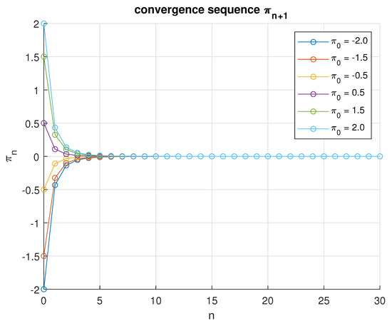
Figure 1. An illustration of the convergence sequence $\left\{{\pi }_{n+1}\right\}$ for various initial values when ${\alpha }_n={\displaystyle \frac{6}{n+6}}$.

Table 1. The convergence sequence $\left\{{\pi }_n\right\}$ is initialized with the values ${\pi }_0=-2,-1.5,-0.5,0.5,1.5,2$.

Number of	${\mathit{\pi }}_0=-2$	${\mathit{\pi }}_0=-1.5$	${\mathit{\pi }}_0=-0.5$	${\mathit{\pi }}_0=0.5$	${\mathit{\pi }}_0=1.5$	${\mathit{\pi }}_0=2$
Iterations, n	${\mathit{\pi }}_{\mathit{n}}$	${\mathit{\pi }}_{\mathit{n}}$	${\mathit{\pi }}_{\mathit{n}}$	${\mathit{\pi }}_{\mathit{n}}$	${\mathit{\pi }}_{\mathit{n}}$	${\mathit{\pi }}_{\mathit{n}}$
1	−0.43243	−0.32433	−0.10811	0.10811	0.32433	0.43243
2	−0.13587	−0.1019	−0.033967	0.033967	0.1019	0.13587
3	−0.05304	−0.03978	−0.01326	0.01326	0.03978	0.05304
6	−0.00651	−0.00488	−0.00162	0.00162	0.00488	0.00651
8	−0.00145	−0.00108	−0.00036	0.00036	0.00108	0.00145
10	−0.00064	−0.00048	−0.00016	0.00016	0.00048	0.00064
13	−0.00023	−0.00017	−0.00005	0.00005	0.00017	0.00023
17	−0.00007	−0.00005	−0.00001	0.00001	0.00005	0.00007
20	−0.00003	−0.00002	−0.00000	0.00000	0.00002	0.00003
23	−0.00001	−0.00001	−0.00000	0.00000	0.00001	0.00001
26	−0.00001	−0.00000	−0.00000	0.00000	0.00000	0.00001
27	−0.00000	−0.00000	−0.00000	0.00000	0.00000	0.00000
30	−0.00000	−0.00000	−0.00000	0.00000	0.00000	0.00000

In the second scenario, the parameters are set as $e_n={\displaystyle \frac{1}{n}}$ and ${\alpha }_n={\displaystyle \frac{9}{n+9}}$, with the same initial values ${\pi }_0=-2,-1.5,-0.5,0.5,1.5,2$. The results of the estimation are summarized in Table 2, and the convergence behavior is illustrated in Figure 2 of the sequence $\left\{{\pi }_{n+1}\right\}$ that converges to $\pi =0$ after 15 iterations.

Table 2. The convergence sequence $\left\{{\pi }_n\right\}$ is initialized with the values ${\pi }_0=-2,-1.5,-0.5,0.5,1.5,2$.

Number of	${\mathit{\pi }}_0=-2$	${\mathit{\pi }}_0=-1.5$	${\mathit{\pi }}_0=-0.5$	${\mathit{\pi }}_0=0.5$	${\mathit{\pi }}_0=1.5$	${\mathit{\pi }}_0=2$
Iterations, n	${\mathit{\pi }}_{\mathit{n}}$	${\mathit{\pi }}_{\mathit{n}}$	${\mathit{\pi }}_{\mathit{n}}$	${\mathit{\pi }}_{\mathit{n}}$	${\mathit{\pi }}_{\mathit{n}}$	${\mathit{\pi }}_{\mathit{n}}$
1	−0.35406	−0.26554	−0.08851	0.08851	0.26554	0.35406
2	−0.08916	−0.06687	−0.02229	0.02229	0.06687	0.08916
3	−0.02801	−0.02101	−0.00700	0.00700	0.02101	0.028015
4	−0.01028	−0.00771	−0.00257	0.00257	0.00771	0.01028
5	−0.00423	−0.00317	−0.00105	0.00105	0.00317	0.00423
6	−0.00191	−0.00143	−0.00047	0.00047	0.00143	0.00191
8	−0.00047	−0.00035	−0.00011	0.00011	0.00035	0.00047
10	−0.00008	−0.00006	−0.00002	0.00002	0.000006	0.00008
12	−0.00003	−0.00002	−0.00000	0.00000	0.00002	0.00003
15	−0.00001	−0.00001	−0.00000	0.00000	0.00001	0.00001
16	−0.00000	−0.00000	−0.00000	0.00000	0.00000	0.00000
20	−0.00000	−0.00000	−0.00000	0.00000	0.00000	0.00000

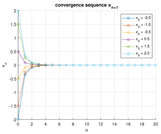
Figure 2. An illustration of the convergence sequence $\left\{{\pi }_{n+1}\right\}$ for various initial values when ${\alpha }_n={\displaystyle \frac{9}{n+9}}$.

In the third scenario, we set ${\alpha }_n={\displaystyle \frac{12}{n+12}}$ while keeping the same values of $e_n={\displaystyle \frac{1}{n}}$ and initial points ${\pi }_0=-2,-1.5,-0.5,0.5,1.5,2$. The numerical results are presented in estimation Table 3, and the convergence behavior is illustrated in Figure 3 of the sequence $\left\{{\pi }_{n+1}\right\}$ which converges to $\pi =0$ after 12 iterations.

Table 3. The convergence sequence $\left\{{\pi }_n\right\}$ is initialized with the values ${\pi }_0=-2,-1.5,-0.5,0.5,1.5,2$.

Number of	${\mathit{\pi }}_0=-2$	${\mathit{\pi }}_0=-1.5$	${\mathit{\pi }}_0=-0.5$	${\mathit{\pi }}_0=0.5$	${\mathit{\pi }}_0=1.5$	${\mathit{\pi }}_0=2$
Iterations, n	${\mathit{\pi }}_{\mathit{n}}$	${\mathit{\pi }}_{\mathit{n}}$	${\mathit{\pi }}_{\mathit{n}}$	${\mathit{\pi }}_{\mathit{n}}$	${\mathit{\pi }}_{\mathit{n}}$	${\mathit{\pi }}_{\mathit{n}}$
1	−0.31185	−0.23389	−0.07796	0.07796	0.23389	0.31185
2	−0.06742	−0.05057	−0.01685	0.01685	0.05057	0.06742
3	−0.01810	−0.01357	−0.00452	0.00452	0.01357	0.01810
4	−0.00568	−0.00426	−0.00142	0.00142	0.00426	0.00568
5	−0.00201	−0.00151	−0.00050	0.00050	0.00151	0.00201
6	−0.00078	−0.00059	−0.00019	0.00019	0.00059	0.00078
8	−0.00015	−0.00011	−0.00003	0.00003	0.00011	0.00015
10	−0.00003	−0.00002	−0.00000	0.00000	0.00002	0.00003
12	−0.00001	−0.00000	−0.00000	0.00000	0.00000	0.00001
13	−0.00000	−0.00000	−0.00000	0.00000	0.00000	0.00000
15	−0.00000	−0.00000	−0.00000	0.00000	0.00000	0.00000

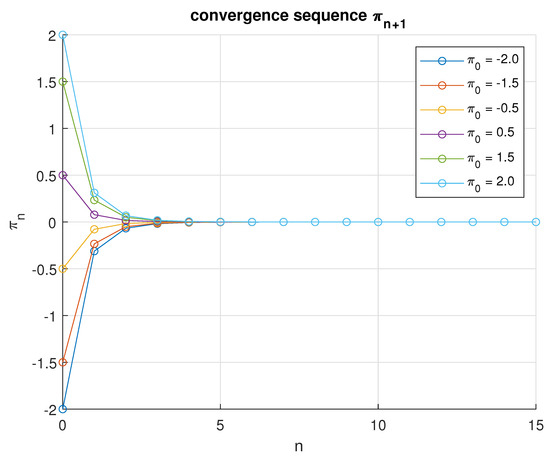
Figure 3. An illustration of the convergence sequence $\left\{{\pi }_{n+1}\right\}$ for various initial values when ${\alpha }_n={\displaystyle \frac{12}{n+12}}$.

In the fourth scenario, we consider $e_n={\displaystyle \frac{1}{n}}$ and ${\alpha }_n={\displaystyle \frac{24}{n+24}}$, while maintaining the same initial values ${\pi }_0=-2,-1.5,-0.5,0.5,1.5,2$. The sequence $\left\{{\pi }_{n+1}\right\}$ converges to the solution $\pi =0$ after seven iterations. The numerical results are summarized in estimation Table 4, and the convergence behavior is illustrated in Figure 4.

Table 4. The convergence sequence $\left\{{\pi }_n\right\}$ is initialized with the values ${\pi }_0=-2,-1.5,-0.5,0.5,1.5,2$.

Number of	${\mathit{\pi }}_0=-2$	${\mathit{\pi }}_0=-1.5$	${\mathit{\pi }}_0=-0.5$	${\mathit{\pi }}_0=0.5$	${\mathit{\pi }}_0=1.5$	${\mathit{\pi }}_0=2$
Iterations, n	${\mathit{\pi }}_{\mathit{n}}$	${\mathit{\pi }}_{\mathit{n}}$	${\mathit{\pi }}_{\mathit{n}}$	${\mathit{\pi }}_{\mathit{n}}$	${\mathit{\pi }}_{\mathit{n}}$	${\mathit{\pi }}_{\mathit{n}}$
1	−0.24433	−0.18324	−0.061082	0.061082	0.18324	0.24433
2	−0.03809	−0.02857	−0.00952	0.00952	0.02857	0.03809
3	−0.00713	−0.0053	−0.00178	0.00178	0.00534	0.00713
4	−0.00154	−0.00115	−0.00038	0.00038	0.00115	0.00154
5	−0.00037	−0.00028	−0.00009	0.00009	0.00028	0.00037
6	−0.00010	−0.00007	−0.00002	0.00002	0.00007	0.00010
7	−0.00002	−0.00002	−0.00000	0.00000	0.00002	0.00002
8	−0.00000	−0.00000	−0.00000	0.00000	0.00000	0.00000
10	−0.00000	−0.00000	−0.00000	0.00000	0.00000	0.00000

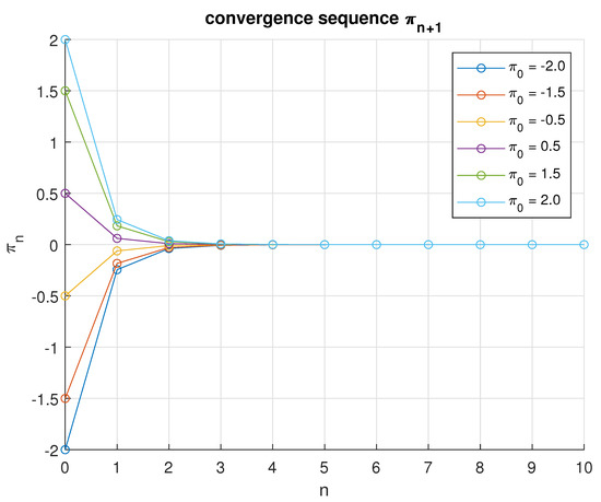
Figure 4. An illustration of the convergence sequence $\left\{{\pi }_{n+1}\right\}$ for various initial values when ${\alpha }_n={\displaystyle \frac{24}{n+24}}$.

In the fifth scenario, we take $e_n={\displaystyle \frac{1}{n}}$ and ${\alpha }_n={\displaystyle \frac{38}{n+38}}$ and the same initial values. We obtain an estimation Table 5 and a convergence graph (Figure 5) of the convergence sequence $\left\{{\pi }_{n+1}\right\}$, which converges to $\pi =0$ (after six iterations).

Table 5. The convergence sequence $\left\{{\pi }_n\right\}$ is initialized with the values ${\pi }_0=-2,-1.5,-0.5,0.5,1.5,2$.

Number of	${\mathit{\pi }}_0=-2$	${\mathit{\pi }}_0=-1.5$	${\mathit{\pi }}_0=-0.5$	${\mathit{\pi }}_0=0.5$	${\mathit{\pi }}_0=1.5$	${\mathit{\pi }}_0=2$
Iterations, n	${\mathit{\pi }}_{\mathit{n}}$	${\mathit{\pi }}_{\mathit{n}}$	${\mathit{\pi }}_{\mathit{n}}$	${\mathit{\pi }}_{\mathit{n}}$	${\mathit{\pi }}_{\mathit{n}}$	${\mathit{\pi }}_{\mathit{n}}$
1	−0.21807	−0.16355	−0.05451	0.05451	0.16355	0.21807
2	−0.02863	−0.02147	−0.00715	0.00715	0.02147	0.02863
3	−0.00436	−0.00327	−0.00109	0.00109	0.00327	0.00436
4	−0.00075	−0.00056	−0.00018	0.00018	0.00056	0.00075
5	−0.00014	−0.00010	−0.00003	0.00003	0.00010	0.00014
6	−0.00003	−0.00002	−0.00000	0.00000	0.00002	0.00003
7	−0.00000	−0.00000	−0.00000	0.00000	0.00000	0.00000
8	−0.00000	−0.00000	−0.00000	0.00000	0.00000	0.00000

Figure 5. An illustration of the convergence sequence $\left\{{\pi }_{n+1}\right\}$ for various initial values when ${\alpha }_n={\displaystyle \frac{38}{n+38}}$.

Now in the final scenario, we take ${\alpha }_n={\displaystyle \frac{98}{n+98}}$ and the same initial values and the same value of $e_n$. Then we get the estimation shown in Table 6 and the convergence graph (Figure 6) of the convergence sequence $\left\{{\pi }_{n+1}\right\}$, which converges at $\pi =0$ (after five iterations).

Table 6. The convergence sequence $\left\{{\pi }_n\right\}$ is initialized with the values ${\pi }_0=-2,-1.5,-0.5,0.5,1.5,2$.

Number of	${\mathit{\pi }}_0=-2$	${\mathit{\pi }}_0=-1.5$	${\mathit{\pi }}_0=-0.5$	${\mathit{\pi }}_0=0.5$	${\mathit{\pi }}_0=1.5$	${\mathit{\pi }}_0=2$
Iterations, n	${\mathit{\pi }}_{\mathit{n}}$	${\mathit{\pi }}_{\mathit{n}}$	${\mathit{\pi }}_{\mathit{n}}$	${\mathit{\pi }}_{\mathit{n}}$	${\mathit{\pi }}_{\mathit{n}}$	${\mathit{\pi }}_{\mathit{n}}$
1	−0.18965	−0.14223	−0.047412	0.047412	0.14223	0.18965
2	−0.01970	−0.01477	−0.00492	0.00492	0.01477	0.01970
3	−0.00222	−0.00166	−0.00055	0.00055	0.00166	0.00222
4	−0.00026	−0.00020	−0.00006	0.00006	0.00020	0.00026
5	−0.00003	−0.00002	−0.00000	0.00000	0.00002	0.00003
6	−0.00000	−0.00000	−0.00000	0.00000	0.00000	0.00000
7	−0.00000	−0.00000	−0.00000	0.00000	0.00000	0.00000

Figure 6. An illustration of the convergence sequence $\left\{{\pi }_{n+1}\right\}$ for various initial values when ${\alpha }_n={\displaystyle \frac{98}{n+98}}$.

To support our main results, six convergence graphs were obtained, demonstrating that the sequence $\left\{{\pi }_n\right\}$ converges to the solution $\pi =0$ under different parameter settings. In the first scenario, convergence occurred within 27 iterations for ${\alpha }_n={\displaystyle \frac{6}{n+6}}$; in the second, within 16 iterations for ${\alpha }_n={\displaystyle \frac{9}{n+9}}$; in the third, within 13 iterations for ${\alpha }_n={\displaystyle \frac{12}{n+12}}$; in the fourth, within 8 iterations for ${\alpha }_n={\displaystyle \frac{24}{n+24}}$; in the fifth, within 7 iterations for ${\alpha }_n={\displaystyle \frac{38}{n+38}}$; and in the sixth and final scenario, convergence was achieved in only 6 iterations for ${\alpha }_n={\displaystyle \frac{98}{n+98}}$.

These findings indicate that a slower decay in the sequence $\left\{{\alpha }_n\right\}$—as in the final scenario—leads to a faster convergence rate. This behavior is observed while maintaining $0\le {\alpha }_n\le 1$ and $0\le e_n\le 1$. Compared to existing methods such as those of Gebrie and Bedene [22] and Rajpoot et al. [23], the proposed inertial extrapolation model exhibits superior convergence performance. The numerical evidence clearly demonstrates that the integration of inertial extrapolation techniques enhances convergence speed and effectiveness in approaching the optimal solution.

8. Conclusions

In this paper, we studied the Yosida–Cayley Variational Inclusion Problem (YCVIP) and the Yosida–Cayley Resolvent Equation Problem (YCREP) within the framework of real-ordered Hilbert spaces, incorporating both multi-valued and single-valued mappings influenced by XOR and XNOR operations. Our primary focus was on the convergence analysis of these problems through the development of an inertial extrapolation scheme. We proposed and rigorously analyzed several iterative algorithms to solve these problems, establishing both the existence and convergence of solutions under suitable conditions on the involved operators and mappings. Furthermore, a comprehensive numerical experiment was presented to demonstrate the computational efficiency and fast convergence of the proposed methods, thereby highlighting their practical relevance and potential for broader applications.

References

- Hartman, P.; Stampacchia, G. On some non-linear elliptic differential-functional equations. Acta Math. 1966, 115, 271–310. [Google Scholar] [CrossRef]
- Fechner, W. Functional inequalities motivated by the Lax–Milgram theorem. J. Math. Anal. Appl. 2013, 402, 411–414. [Google Scholar] [CrossRef]
- Rockafellar, R. Monotone operators and the proximal point algorithm. SIAM J. Cont. Optim. 1976, 14, 877–898. [Google Scholar] [CrossRef]
- Kegl, M.; Butinar, B.J.; Kegl, B. An efficient gradient-based optimization algorithm for mechanical systems. Commun. Numer. Methods Eng. 2002, 18, 363–371. [Google Scholar] [CrossRef]
- Salahuddin. Solutions of Variational Inclusions over the Sets of Common Fixed Points in Banach Spaces. J. Appl. Non. Dy. 2021, 11, 75–85. [Google Scholar]
- Akram, M.; Dilshad, M. A Unified Inertial Iterative Approach for General Quasi Variational Inequality with Application. Fractal Fract. 2022, 6, 395. [Google Scholar] [CrossRef]
- AlNemer, G.; Rehan Ali, R.; Farid, M. On the Strong Convergence of Combined Generalized Equilibrium and Fixed Point Problems in a Banach Space. Axioms 2025, 14, 428. [Google Scholar] [CrossRef]
- Sitthithakerngkiet, K.; Rehman, H.U.; Ioannis, K.; Argyros, I.K.; Seangwattana, T. Strong convergence of dual inertial fixed point algorithms for computing fixed points over the solution set of a variational inequality problem in real Hilbert spaces. Rend. Circ. Mat. Di Palermo 2025, 74, 82. [Google Scholar] [CrossRef]
- Daoud, S.M.; Shehab, M.; Al-Mimi, M.H.; Abualigah, L.; Zitar, A.R.; Shambour, M.K.Y. Gradient-Based Optimizer (GBO): A Review, Theory, Variants, and Applications. Arch. Comput. Methods Eng. 2023, 30, 2431–2449. [Google Scholar] [CrossRef]
- Rehman, H.U.; Sitthithakerngkiet, K.; Seangwattana, T. Dual-Inertial Viscosity-Based Subgradient Extragradient Methods for Equilibrium Problems Over Fixed Point Sets. Math. Methods Appl. Sci. Anal. Appl. 2025, 48, 6866–6888. [Google Scholar] [CrossRef]
- Altbawi, S.M.A.; Khalid, S.B.A.; Mokhtar, A.S.B.; Hussain Shareef, H.; Husain, N.; Ashraf Yahya, A.; Haider, S.A.; Moin, L.; Alsisi, H.R. An Improved Gradient-Based Optimization Algorithm for Solving Complex Optimization Problems. Processes 2023, 11, 498. [Google Scholar] [CrossRef]
- Hassouni, A.; Moudafi, A. A perturbed algorithm for variational inclusions. J. Math. Anal. Appl. 1994, 185, 706–712. [Google Scholar] [CrossRef]
- Ahmad, I.; Irfan, S.S.; Farid, M.; Shukla, P. Nonlinear ordered variational inclusion problem involving XOR operation with fuzzy mappings. J. Inequal. Appl. 2020, 2020, 36. [Google Scholar] [CrossRef]
- Ahmad, I.; Pang, C.T.; Ahmad, R.; Ishtyak, M. System of Yosida inclusions involving XOR-operation. J. Nonlinear Convex Anal. 2017, 18, 831–845. [Google Scholar]
- Li, H.G.; Pan, X.B.; Deng, Z.Y.; Wang, C.Y. Solving GNOVI frameworks involving (γG, λ)-weak-GRD set-valued mappings in positive Hilbert spaces. Fixed Point Theory Appl. 2014, 2014, 146. [Google Scholar] [CrossRef]
- Iqbal, J.; Rajpoot, A.K.; Islam, M.; Ahmad, R.; Wang, Y. System of Generalized variational inclusions involving Cayley operators and XOR-operation in q-uniformly smooth Banach spaces. Mathematics 2022, 10, 2837. [Google Scholar] [CrossRef]
- Ali, I.; Ahmad, R.; Wen, C.F. Cayley inclusion problem involving XOR-operation. Mathematics 2019, 7, 302. [Google Scholar] [CrossRef]
- Iqbal, J.; Wang, Y.; Rajpoot, A.K.; Ahmad, R. Generalized Yosida inclusion problem involving multi-valued operator with XOR operation. Demonstr. Math. 2024, 57, 20240011. [Google Scholar] [CrossRef]
- Noor, M.A. Generalized set-valued variational inclusions and resolvent equations. J. Math. Anal. Appl. 1998, 228, 206–220. [Google Scholar] [CrossRef]
- Polyak, B.T. Some methods of speeding up the convergence of iteration methods. USSR Comput. Math. Math. Phys. 1964, 4, 1–17. [Google Scholar] [CrossRef]
- Chang, S.; Yao, J.C.; Wang, L.; Liu, M.; Zhao, L. On the inertial forward-backward splitting technique for solving a system of inclusion problems in Hilbert spaces. Optimization 2021, 70, 2511–2525. [Google Scholar] [CrossRef]
- Gebrie, A.G.; Bedane, S.D. A simple computational algorithm with inertial extrapolation for generalized split common fixed point problems. Heliyon 2021, 7, e08373. [Google Scholar] [CrossRef] [PubMed]
- Rajpoot, A.K.; Istiak, M.; Ahmed, R.; Wang, Y.; Yao, J.C. Convergence analysis for Yosida variational inclusion problem with its corresponding Yosida resolvent equation problem through inertial extrapolation scheme. Mathematics 2023, 11, 763. [Google Scholar] [CrossRef]
- Noor, M.A.; Noor, K.I. General bivariational inclusions and iterative methods. Int. J. Nonlinear Anal. Appl. 2023, 14, 309–324. [Google Scholar]
Disclaimer/Publisher’s Note: The statements, opinions and data contained in all publications are solely those of the individual author(s) and contributor(s) and not of MDPI and/or the editor(s). MDPI and/or the editor(s) disclaim responsibility for any injury to people or property resulting from any ideas, methods, instructions or products referred to in the content. |
© 2025 by the authors. Licensee MDPI, Basel, Switzerland. This article is an open access article distributed under the terms and conditions of the Creative Commons Attribution (CC BY) license (https://creativecommons.org/licenses/by/4.0/).