Abstract
The increasing complexity of manufacturing processes demands accurate defect prediction and interpretable insights into the causes of quality issues. This study proposes a methodology integrating machine learning, clustering, and Explainable Artificial Intelligence (XAI) to support defect analysis and quality control in industrial environments. Using a dataset based on empirical industrial distributions, we train an XGBoost model to classify high- and low-defect scenarios from multidimensional production and quality metrics. The model demonstrates high predictive performance and is analyzed using five XAI techniques (SHAP, LIME, ELI5, PDP, and ICE) to identify the most influential variables linked to defective outcomes. In parallel, we apply Fuzzy C-Means and K-means to segment production data into latent operational profiles, which are also interpreted using XAI to uncover process-level patterns. This approach provides both global and local interpretability, revealing consistent variables across predictive and structural perspectives. After a thorough review, no prior studies have combined supervised learning, unsupervised clustering, and XAI within a unified framework for manufacturing defect analysis. The results demonstrate that this integration enables a transparent, data-driven understanding of production dynamics. The proposed hybrid approach supports the development of intelligent, explainable Industry 4.0 systems.
Keywords:
Explainable Artificial Intelligence (XAI); defect prediction; manufacturing quality control; mathematical evaluation XAI; ISO 9001 compliance MSC:
68T20; 62P30
1. Introduction
In any industrial production process, quality management and quality control are fundamental components, especially when dealing with perishable products or high-precision manufacturing. Ensuring consistent quality is essential to guarantee product safety, enhance customer satisfaction, and comply with quality regulations. In this respect, international standards such as ISO 9001 provide an integrated framework for quality management systems, with an emphasis on process monitoring, defect prevention, and continuous improvement [1].
Across diverse sectors, from the food industry to porcelain and glass manufacturing, the overarching goal is to deliver products that meet predefined quality thresholds while minimizing production costs and waste. Based on direct observations from visits to manufacturing plants in both the food and materials sectors, quality control efforts are focused on achieving minimum defect rates without incurring excessive sampling or reprocessing costs. In these settings, sample-based inspections, through either physical extraction or visual analysis, are key to monitoring the state of production in real time.
When systematically recorded and analyzed, such sampling data can support the early detection of anomalies and inform decisions related to defect prevention and process optimization. In recent years, the integration of machine learning (ML) into industrial quality control systems has enabled predictive models that anticipate high-risk scenarios using multidimensional process indicators [2,3]. However, the complexity and opacity of many artificial intelligence models, particularly black-box or deep learning models, pose significant challenges for trust, regulation, and practical deployment [4].
To address this, Explainable Artificial Intelligence (XAI) has emerged as a set of techniques aimed at making black-box models more transparent and interpretable. By attributing predictions to input features, XAI helps stakeholders understand and validate model behavior [5]. While XAI methods such as SHAP, LIME, and ELI5 are increasingly used in domains like finance, human resources, and healthcare [6,7,8], comparative studies with a formal and interpretable mathematical basis remain limited in the manufacturing field.
This paper presents a mathematically grounded evaluation of five XAI techniques, SHAP, LIME, ELI5, PDP, and ICE, in the context of defect prediction in manufacturing. The study uses the “manufacturing_defect_dataset.csv”, a structured dataset commonly employed for benchmarking machine learning models in industrial scenarios. The dataset reflects realistic manufacturing behavior by sampling from empirical distributions observed in production systems, enabling the development of a robust and generalizable evaluation framework while maintaining interpretability and domain alignment [9].
In addition to supervised defect prediction, we also apply Fuzzy C-Means clustering to segment production conditions based on similarity in the process variables. Although not strictly an XAI method, fuzzy clustering contributes to the overall interpretability framework by enabling the analysis of latent operational profiles. These clusters are subsequently interpreted using XAI, allowing for comparison between predictive and structural explanations [10].
By combining industrial relevance with mathematical rigor, our goal is to contribute a transparent, consistent, and interpretable methodology for quality control systems based on AI, aligned with the operational and normative demands of modern manufacturing. This framework, which integrates predictive modeling, fuzzy clustering, and explainability, supports decision-making in quality management and provides a generalizable and adaptable approach applicable to a wide range of industrial manufacturing scenarios.
The remainder of this paper is structured as follows: Section 2 provides a review of the most relevant literature, organized into four key areas: deep learning for fault detection, the integration of XAI into industrial applications, the use of fuzzy clustering for production profiling, and the current lack of unified frameworks that combine these techniques. Section 3 presents the dataset, the preprocessing steps, and the dual experimental design involving supervised defect prediction and fuzzy clustering. It also introduces the complete methodological framework of the study, including the mathematical foundations and evaluation procedures applied to the explainability techniques. Section 4 reports the experimental results and provides a comparative discussion of the explanatory value and robustness of each method. Section 5 reflects the contributions, limitations, and potential extensions of this work and proposes directions for future research. Finally, Section 6 offers concluding remarks.
2. Related Work
Recent advances in Artificial Intelligence (AI) and machine learning have led to significant progress in quality control and fault detection processes in industrial manufacturing. Deep learning models have shown high predictive performance in identifying defects from complex production data in domains such as electronics, automotive, and high-precision manufacturing. However, these models often lack explainability and interpretability, which are key in environments requiring traceability and regulatory compliance.
To overcome these limitations, Explainable Artificial Intelligence (XAI) techniques have been developed and adapted to industrial contexts, enabling greater transparency in model behavior and supporting informed decision-making by domain experts. In parallel, fuzzy clustering methods such as Fuzzy C-Means (FCM) provide a complementary approach by enabling segmentation of both intermediate and final product conditions. These methods are particularly useful in processes characterized by degrees of membership, where classifications are rarely binary or clear-cut [11,12].
This section reviews the state of the art across four dimensions relevant to our study: first, deep learning approaches for fault detection in manufacturing; second, the integration of XAI in industrial applications; third, conventional and fuzzy clustering for production profiling and defect pattern discovery; and finally, the limited, but growing, body of work attempting to combine these paradigms into a unified framework.
2.1. Deep Learning + Fault Detection + Manufacturing
Over the past decade, deep learning has become a leading approach to fault detection in industrial manufacturing systems. Its ability to process non-linear and high-dimensional data makes it particularly well suited to identify subtle patterns associated with quality deviations in sectors such as electronics, automotive and precision engineering.
Scientific interest in the application of deep learning to manufacturing fault detection has experienced steady growth since 2017. A preliminary search conducted in the Web of Science (WOS) database reveals a total of 292 publications and over 5800 citations related to this topic. This trend underscores the consolidation of deep learning as a key approach for predictive quality assurance in industrial environments, as shown in Figure 1.
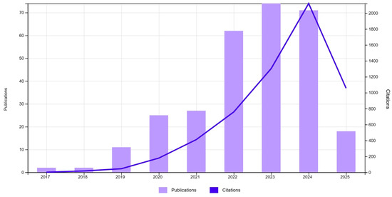
Figure 1.
WOS publications (292) and citations. TS = (“deep learning”) AND TS = (“fault detection”) AND TS = (“manufacturing” OR “industry” OR “production”).
Numerous studies have shown that the use of convolutional neural networks (CNNs) and recurrent neural networks (RNNs) can effectively detect defects in production, all in real time [13,14,15,16,17,18,19]. As these models grow in complexity, being black-box models, interpretability becomes a relevant need, especially in regulated environments where traceability and interpretability are essential for compliance and operational validation.
This limitation motivates the integration of explainable AI methods, which will be addressed in the following section.
2.2. Explainable AI (XAI) + Manufacturing
As machine learning and deep learning models become more widely used in industrial applications, understanding the logic behind their predictions is critical for quality control, regulatory compliance, and stakeholder confidence.
A review of the underlying literature related to this topic shows a clear upward trend. The number of publications combining XAI with machine learning in manufacturing contexts has grown since 2020, reaching a total of 226 publications and 2820 citations. The year 2024 marked the peak, with almost 90 publications and more than 1200 citations, confirming the strategic interest in interpretive AI for industrial quality systems, as shown in Figure 2.
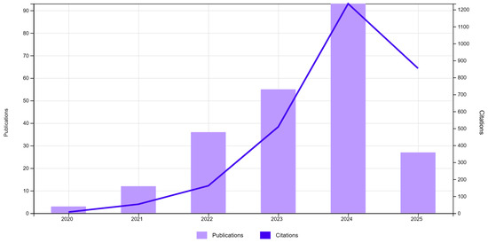
Figure 2.
WOS publications (226) and citations. TS = (“explainable AI” OR “XAI”) AND TS = (“manufacturing” OR “production” OR “quality control”) AND TS = (“machine learning” OR “deep learning”).
This increase reflects a shift in industrial AI priorities from purely predictive accuracy to transparent and defensible decision-making frameworks, especially in regulated or high-risk environments [20,21,22,23]. However, despite the growing body of work, most XAI applications focus exclusively on supervised learning, with limited exploration of its potential in unsupervised or fuzzy modeling approaches, a gap that this paper aims to address.
2.3. Fuzzy C-Means + Product Classification OR Quality
Fuzzy clustering methods, in particular Fuzzy C-Means (FCM), have a high ability to model uncertainty and overlapping class boundaries in data [24]. Unlike rigid clustering methods, FCM allows observations to belong to multiple clusters with varying degrees of membership, making it particularly suitable for complex production environments where process conditions are often ambiguous and continuous rather than discrete.
Despite its theoretical advantages, the application of FCM in production quality measurement remains limited, as illustrated in Figure 3; the number of studies is limited to a total of 68 publications and a total of 1293 citations. The first works on FCM date back to 1990 [25], and its use in industrial contexts did not start to gain traction until after 2015 [26]. Between 2019 and 2024, a small but steady stream of studies emerged [27,28,29,30]. This confirms a growing, albeit niche, interest in leveraging fuzzy methods to address quality control challenges.
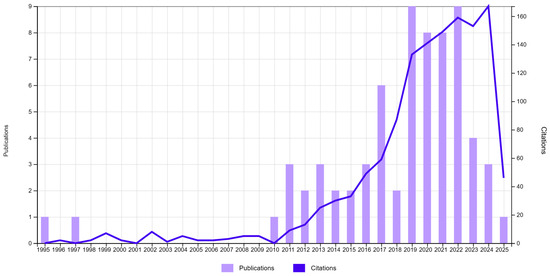
Figure 3.
WOS publications (68) and citations. TS = (“fuzzy c-means” OR “fuzzy clustering”) AND TS = (“product classification” OR “manufacturing”).
These works typically apply FCM to problems such as fault detection, condition monitoring, or process segmentation [31,32,33]. However, most studies use FCM as a standalone tool for classification or clustering, without coupling it with explainable AI techniques. The integration of FCM with modern interpretability frameworks remains virtually unexplored, representing a methodological gap that this article seeks to address.
2.4. Joint Use of XAI + Fuzzy Clustering + ML in Industry
The use of methodologies related to explainable AI (XAI) and fuzzy clustering (FCM) have been developed and tested in various studies, demonstrating their potential application in manufacturing process environments, although both methodologies are typically used independently. The combination of both technologies can help in classifying processes and understanding interpretability mechanisms in supervised algorithms, but remains unexplored. This is especially striking considering the growing need for interpretable and adaptive AI systems in modern industrial environments, where uncertainty, variability, and liability coexist.
To assess the current state of research, we conducted a comprehensive search of the Web of Science database using the following combined query:
TS = (“explainable AI” OR “XAI”) AND TS = (“fuzzy c-means” OR “fuzzy clustering”) AND TS = (“manufacturing” OR “industry”) AND TS = (“deep learning” OR “machine learning”).
The search yielded no results, confirming that there are no published studies to date that explicitly combine these four components within a single methodological pipeline. This absence highlights a clear research gap and underscores the novelty of our proposed framework, which integrates supervised defect prediction using machine learning (XGBoost), fuzzy clustering of production profiles (FCM), and explanation layers applied to both processes using multiple XAI techniques.
The work presented in this paper contributes to bridging the gap between supervised and unsupervised models and interpretability, allowing for a more comprehensive and transparent approach to quality control in manufacturing.
3. Materials and Methods
This section outlines the materials and methodological procedures implemented in the proposed study. It includes a detailed description of the dataset used, the preprocessing steps applied, and a dual framework for defect prediction and fuzzy classification in manufacturing. The aim is to provide a transparent and replicable process that integrates supervised learning, unsupervised clustering, and explanation methods under a unified evaluation strategy.
We first introduce the dataset, which contains structured records of manufacturing conditions and defect outcomes. Following this, we describe the data preparation procedures, including normalization and partitioning for both predictive and clustering tasks.
The core of our methodology is built on two complementary tracks. The first involves training a predictive model using the XGBoost algorithm to classify high- and low-defect scenarios, followed by the application of several Explainable AI (XAI) techniques to interpret the model’s decisions. The second track applies K-means and Fuzzy C-Means clustering to segment production conditions into latent operational profiles. These cluster assignments are subsequently used as targets in a supervised XGBoost classifier, whose outputs are interpreted using XAI techniques (SHAP and LIME) to reveal the most influential features driving each profile.
Finally, we interpret the outputs of both modeling tracks using multiple XAI techniques (SHAP, LIME, ELI5, PDP, and ICE), focusing on identifying consistent explanatory patterns across predictive and clustering-based insights. While a formal mathematical evaluation of explainability methods is left as future work, this dual approach supports a transparent and interpretable understanding of quality-related factors in manufacturing, as summarized in Figure 4.
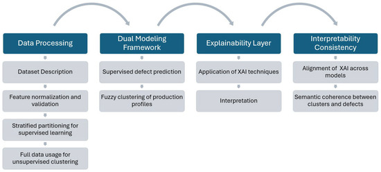
Figure 4.
Methodological workflow for interpretable defect analysis in manufacturing.
3.1. Dataset and Preprocessing
The dataset used in this study is a structured collection of 3240 observations related to industrial manufacturing processes. It includes both operational and quality-related variables, such as production volume, cost metrics, supplier performance, maintenance activity, energy efficiency, and defect rates. The objective is to model and analyze how these variables are associated with the presence or absence of product defects.
Let denote the dataset used in this study, where each instance represents a 16-feature vector of production-related variables, and is the binary label indicating whether the product is defective or not .
The target variable “DefectStatus” exhibits a pronounced class imbalance, with 2723 defective samples and 517 non-defective samples , representing 84.0% and 16.0% of the dataset, respectively. This imbalance was mitigated by using stratified sampling and class-sensitive performance metrics during model training and evaluation.
3.1.1. Feature Normalization
To ensure compatibility across modeling techniques and the dominance of variables due to scale differences, all numerical features were normalized to the unit interval using Min-Max scaling:
This transformation was applied independently to each feature , where denotes the vector of all values for feature .
3.1.2. Partitioning Strategy
The dataset was partitioned as follows:
- Supervised learning (XGBoost): an 80/20 stratified split was performed to produce training and testing sets and , preserving the proportion of defective and non-defective samples.
- Unsupervised learning (Fuzzy C-Means): the entire feature matrix was used for clustering, ignoring the target variable.
3.1.3. Dimensionality Check
To verify dimensional soundness, Principal Component Analysis (PCA) was applied to to verify that the majority of variance was distributed across multiple components and to ensure there were no collinear or redundant features. PCA was used solely for exploratory purposes and not as part of the modeling pipeline.
This preprocessing pipeline ensures that the dataset is ready for both supervised defect prediction and fuzzy segmentation, maintaining integrity and mathematical validity across all phases of the methodological framework.
3.2. Dual Modeling Framework
This section describes the two complementary modeling tracks developed in this study: (1) supervised learning for defect prediction, and (2) unsupervised fuzzy clustering for production profile discovery. Both approaches use the same input features, previously normalized and preprocessed, but pursue distinct objectives, predictive classification and structural segmentation, respectively.
3.2.1. Supervised Defect Prediction (XGBoost)
To predict defective outcomes, we trained a binary classification model using the Extreme Gradient Boosting (XGBoost) algorithm [34]. Formally, given a dataset , where and , XGBoost builds an ensemble of classification trees that approximate a function , mapping input features to a predicted probability of defect:
where is the logistic sigmoid function and is the space of classification trees. The final prediction is thresholded (e.g., at 0.5) to produce a binary outcome.
The model is trained to minimize the regularized binary cross-entropy loss as follows:
where is the logistic loss, and is a regularization term penalizing the complexity of each tree.
Model parameters such as learning rate, tree depth, and number of estimators were tuned via cross-validation. Performance metrics included AUC-ROC, accuracy, precision, recall, and F1-score to address the class imbalance in the dataset.
3.2.2. Unsupervised Fuzzy Clustering (Fuzzy C-Means)
In parallel with supervised learning, we applied two unsupervised clustering algorithms, Fuzzy C-Means (FCM) and K-means, to identify latent operational profiles within the manufacturing data. These techniques allow the segmentation of production instances based solely on process variables, excluding the defect label.
Fuzzy C-Means (FCM) enables each observation to belong to multiple clusters with varying degrees of membership , providing a soft partitioning of the input space [24]. The algorithm minimizes the following objective function:
where
- is the centroid of cluster ,
- is the fuzzifier parameter (we set ),
- denotes the Euclidean norm.
The FCM alternates between updating the membership matrix and the cluster centroids until convergence. The number of clusters was selected by maximizing the Partition Coefficient (PC) and the Fuzzy Silhouette Index (FSI), ensuring stability and interpretability.
K-means, by contrast, produces a hard partition of the dataset by assigning each observation to the nearest cluster centroid. It minimizes intra-cluster variance and was used to validate and complement the fuzzy results.
Both clustering strategies offer alternative structural views of the manufacturing process. These clusters were later interpreted with XAI methods and compared to the supervised classification results to evaluate alignment between structural segmentation and defect-driven predictions.
3.3. Explainability Layer
To increase the transparency and accountability of the predictive and clustering models, we implemented a layer of post hoc explainability using five techniques from the Explainable Artificial Intelligence (XAI) domain as follows: SHAP, LIME, ELI5, PDP and ICE.
This explainability layer was independently applied to both components of the framework. In the supervised track, it was used to analyze the contribution of each input feature to the XGBoost classifier’s prediction of defect likelihood, enabling model auditing and the validation of learned decision rules against domain knowledge. In the unsupervised track, the same techniques were employed to interpret the clustering results, identifying the features that most strongly influence the degree of membership of each instance to the discovered clusters. Thus, explainability serves a dual purpose: it supports both the auditing of the predictive model and the characterization of latent production profiles, enhancing the practical relevance of the framework for quality control and operational decision-making.
Each XAI technique provides distinct perspectives on feature relevance.
3.3.1. SHAP (Shapley Additive Explanations)
SHAP is an additive feature attribution method grounded in cooperative game theory. It quantifies the contribution of each input feature to a specific prediction by computing Shapley values, originally formulated to fairly distribute payouts among players cooperating in a coalition [35].
Given a model , and a feature index , the SHAP value for feature is defined as
where is the set of all features and represents a subset of features not including . This expression computes the average marginal contribution of feature across all possible subsets , ensuring fairness in feature attribution as derived from cooperative game theory.
SHAP satisfies the following three key properties desirable in explanation models:
- Local accuracy (additivity):
- Consistency: if a model changes such that a feature’s contribution increases or remains the same regardless of other features, its SHAP value will not decrease.
- Missingness: if a feature is missing in all coalitions (not used in the model), its SHAP value is zero.
In practice, SHAP is often computed using approximations to reduce the exponential computational cost of evaluating all feature coalitions.
3.3.2. LIME (Local Interpretable Model-Agnostic Explanations)
LIME is a post hoc interpretability method designed to explain the predictions of any black-box model by approximating it locally with an interpretable surrogate model. The central idea is to perturb the input data around a target instance and learn a simpler model that mimics the behavior of the original model in that local neighborhood [36].
Given a black-box model and an instance , LIME constructs a local surrogate model , where is a class of interpretable models (e.g., linear regressions or decision trees), by minimizing the following objective function:
where is a local fidelity loss function that measures how close approximates in the vicinity of ; is a proximity kernel that defines the locality around , assigning higher weights to samples close to ; is a regularization term enforcing the simplicity (e.g., sparsity) of the surrogate model .
A typical form of the loss is the weighted squared error:
Here, is a set of perturbed samples generated around , often by randomly modifying feature values. LIME thus seeks an interpretable model that approximates well in the region defined by .
LIME is model-agnostic, which means that it can be applied to any classifier or regressor without the need to access the model’s internal parameters or gradients. However, it has several limitations, including the following:
- Instability: small perturbations in x or the sampling process can lead to different explanations.
- Sensitivity to kernel width: the choice of (often exponential or Gaussian) heavily influences the local behavior.
- Approximation error: g may fail to capture complex interactions present in f, especially in high-dimensional spaces.
Despite these limitations, LIME remains a widely used tool for gaining insight into individual predictions, particularly in domains requiring transparency for regulatory or ethical reasons.
3.3.3. ELI5 (Explain Like I’m Five)
ELI5 is an interpretability library designed to provide human-readable explanations for machine learning models, particularly those based on decision trees and linear classifiers. It offers practical tools to de-compose model predictions into feature-level contributions, enabling both global and local interpretability [37].
For linear models such as Logistic Regression, ELI5 computes the contribution of each feature directly from the model coefficients as follows:
where is the weight (coefficient) associated with feature , and is the value of feature in the input instance .
The model’s prediction is then given by
where is the sigmoid activation function and is the model intercept. ELI5 explicitly displays the contribution of each term , enabling users to understand how each feature influences the final decision.
For models like XGBoost, ELI5 uses a method called “decision path tracing”. This approach tracks the specific path that an instance follows through a decision tree and aggregates the information gain contributions of each split.
The local contribution of feature is computed as follows:
where denotes the set of trees traversed by the instance , and is the information gained attributed to feature in tree .
This mechanism enables the estimation of marginal contributions of each feature to the individual prediction , even in complex ensemble architectures. ELI5 offers high compatibility with widely used machine learning models such as XGBoost, LightGBM, and scikit-learn. Its explanations are straightforward and easily understood by human users, and it provides detailed visualizations that support both local (instance-level) and global interpretations of model behavior.
ELI5 provides a practical, accessible, and technically effective tool for understanding machine learning model behavior, especially in production environments where transparency and auditability are essential.
3.3.4. PDP (Partial Dependence Plots)
Partial Dependence Plots (PDPs) are a global interpretability technique used to visualize how one or more input variables influence the average model prediction, while marginalizing the other variables. PDP offers an aggregated perspective of model behavior [38].
Let denote the trained predictive model, where represents the input features. For a specific feature , the partial dependence function is defined as follows:
where denotes all variables except , and the expectation is computed over the distribution of the dataset.
In practice, this expectation is approximated empirically by
This involves replacing the value of feature with a fixed value across all observations and averaging the resulting predictions.
PDPs are typically visualized as a curve showing on the y-axis against varying values of on the x-axis. For two variables, a 3D surface or heatmap can be generated to show joint effects.
PDPs are particularly effective in detecting non-linear relationships between input features and model predictions, offering insight into the marginal average effect of individual variables. As a model-agnostic technique, they are applicable to both interpretable and black-box architectures. PDPs assume that the feature under analysis is independent of the remaining input variables, an assumption that may not be held in real-world scenarios and can lead to misleading interpretations. Moreover, when used in a univariate manner, they fail to capture feature interactions, which are often critical in complex models. Additionally, the presence of multicollinearity may obscure the true marginal effects, complicating the interpretation. Despite these limitations, PDP is a tool that helps to visualize the overall behavior of models, especially in the context of auditing, interpretability, and validation of complex predictive systems.
3.3.5. ICE (Individual Conditional Expectation)
Individual Conditional Expectation (ICE) plots are a model-agnostic explainability technique designed to provide instance-level visualizations of how changes in a single input feature affect the prediction, while keeping all other features fixed. Unlike Partial Dependence Plots (PDP), which average over the dataset, ICE plots retain the heterogeneity of individual predictions, making them especially useful for identifying interactions and non-linear effects in complex models [38].
Let denote the predictive model, where is a vector of input features. For a given observation , the ICE function for the feature is defined as follows:
where denotes all features of instance except for the feature , is varied across its range while the remaining features are held fixed, and is the output of the trained prediction function.
Each ICE curve corresponds to a single instance and shows the evolution of the predicted outcome as a function of . When averaged across all instances, ICE recovers the PDP as follows:
This relationship highlights the individual-level granularity of ICE, in contrast with the aggregated view provided by PDP.
ICE plots provide a granular, instance-level visualization of how model predictions change when a single input feature varies while others remain fixed. By displaying one curve per observation, ICE enables the detection of heterogeneous feature effects, non-linear interactions, and potential outliers, insights often obscured in aggregated methods like PDP. This approach preserves individual interpretability, is compatible with any black-box model, and is particularly valuable in validating models across diverse subpopulations. However, ICE plots can become visually complex in large datasets and rely on the assumption of conditional independence, which may be violated when input features are highly correlated. ICE is a powerful tool for exploring model behavior in high-stakes settings requiring transparency and fairness.
3.3.6. Interpretation Strategy
The interpretability insights provided by the XAI techniques are used to support two complementary objectives. First, we analyze the predictions made by the supervised XGBoost classifier, aiming to identify which features most influence the likelihood of defects. This facilitates model auditing and enhances trust in automated decisions. Second, we apply interpretability tools to the clustering results, allowing us to characterize the latent production profiles discovered by K-means and Fuzzy C-Means algorithms. By interpreting the degree of membership of each instance to different clusters, we aim to uncover relevant operational patterns and validate the consistency between predictive and structural perspectives.
This dual interpretability approach ensures that both the classification of defect status and the segmentation of production conditions are transparent, explainable, and aligned with domain knowledge.
3.4. Comparative and Mathematical Evaluation (Conceptual Framework)
To support a future formal assessment of explainability methods in manufacturing, we propose a mathematical evaluation framework structured around the following three complementary axes: (1) consistency and convergence, (2) formal interpretability properties, and (3) quantitative informativeness metrics.
While this framework is conceptually introduced in the present work, its numerical implementation is left for future research. The current analysis focuses on qualitative coherence between supervised predictions, clustering results, and explanation outputs, laying the foundation for rigorous comparative validation in subsequent studies.
3.4.1. Consistency and Convergence
Let denote the attribution vector for instance generated by explanation method . Given samples , we define the ranking consistency between two methods and as the average Spearman correlation as follows:
Additionally, intra-method stability is defined by adding small noise to the input and computing the norm deviation as follows:
3.4.2. Formal Properties
We also outline theoretical criteria for evaluating XAI methods:
- Additivity (e.g., SHAP)
- Local Fidelity (e.g., LIME)
- Implementation Invariance
- Feature Interaction Awareness
While qualitative in nature, these properties can be verified empirically through regression tests (e.g., local surrogate fit R2) or by comparing explanation stability across equivalent models.
3.4.3. Quantitative Metrics
A full benchmarking framework could be incorporated as follows:
- Entropy of feature attributions, as defined in Equation (16), is used to quantify the concentration or dispersion of importance scores across features.
- Rank correlation (Spearman’s ) across methods and across perturbed inputs, as a measure of coherence and robustness.
- Stability Index to evaluate resistance to minor input fluctuations.
This framework, though not yet fully implemented, provides a formal foundation for future quantitative evaluation of XAI techniques in high-stakes, quality-critical manufacturing contexts. It is important to note that the present framework does not address temporal dynamics or system trajectories in a control–theoretic sense. The goal is not to model the evolution of the manufacturing process over time, but rather to evaluate the consistency and robustness of explanation outputs under controlled perturbations. While some of the proposed metrics, such as entropy and explanation instability, may conceptually resemble stability indicators (e.g., Lyapunov-like functions), they are applied in this study in a static, non-dynamical context [39]. Future studies may explore these analogies within a formal mathematical setting.
4. Results
This section presents the experimental results of the dual modeling framework, which is applied to both defect prediction and production profile segmentation. The analysis is structured in two parts, as follows: the first addresses supervised learning for defect classification, while the second explores clustering of manufacturing conditions. In both tracks, explainability techniques are employed to analyze model outputs, assess feature relevance, and evaluate consistency with domain knowledge.
4.1. Supervised Defect Prediction and Explainability
This subsection presents the performance results of the XGBoost classifier in predicting defect status (binary target), followed by interpretability analysis using XAI techniques. We evaluate classification accuracy, precision, recall, and AUC, and then examine the relevance and consistency of feature attributions. The goal is to validate whether the model’s decision-making aligns with plausible manufacturing logic.
4.1.1. Exploratory Data Analysis (EDA)
Before training any predictive or clustering model, a preliminary exploration of the dataset was conducted to assess basic statistical properties, inter-variable relationships, and potential redundancies. While EDA encompasses a wide variety of statistical and visualization techniques, in this study we apply a focused EDA approach centered on Pearson correlation analysis and heatmap visualization, as these allow a concise inspection of the linear associations among process variables and their relation to defect occurrence. This exploratory step helps identify which features might be most relevant for supervised and unsupervised learning tasks and supports the later interpretability analysis by revealing preliminary associations within the data.
The data used for the initial experiments is the open-access Manufacturing Defects dataset [9]. The variables representing process parameters and defect indicators are detailed in Table 1.

Table 1.
Manufacturing Defects dataset features.
“DefectStatus” is the target variable, with a value of 1 if the product is defective and 0 otherwise. All features are numerical and represent key parameters from the manufacturing process. These include production metrics (e.g., “ProductionVolume”, “ProductionCost”), quality indicators (e.g., “SupplierQuality”, “QualityScore”), efficiency metrics (e.g., “EnergyEfficiency”, “WorkerProductivity”), and incident logs (e.g., “SafetyIncidents”, “MaintenanceHours”). The dataset contains no missing or invalid entries, and all variables have been validated and normalized for model compatibility.
Exploratory Data Analysis (EDA) was used to determine the most influential features potentially associated with defect occurrence. Figure 5 presents a Pearson correlation heatmap summarizing the linear relationships between variables. The full matrix is shown (both upper and lower triangles) to maintain standard exploratory data analysis conventions and facilitate visual inspection of pairwise relationships across all features.
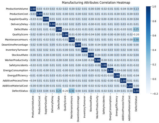
Figure 5.
Correlation matrix for manufacturing attributes.
The following is a summary of the exploratory data analysis (EDA) results:
- The dataset is complete and well-structured, with no missing values or inconsistent formats.
- The strongest positive correlations with the target variable (“DefectStatus”) are observed for “MaintenanceHours” (0.30) and “DefectRate” (0.25).
- The strongest negative correlations with “DefectStatus” are “QualityScore” (−0.20) and “ProductionVolume” (−0.13).
- Most variables exhibit low pairwise correlations, suggesting the presence of non-linear or multivariate interactions, which supports the use of tree-based models and post hoc interpretability techniques.
- No feature displays strong collinearity; all correlation values remain below 0.35, indicating minimal redundancy and avoiding multicollinearity issues.
- Features with minimal variance or negligible association with the target may be considered for exclusion or dimensionality reduction prior to training.
- Higher values of “MaintenanceHours” and “DefectRate” are consistently associated with increased defect probability, while lower “QualityScore” is frequently linked to defective outputs.
- “SafetyIncidents” and “WorkerProductivity” show weak direct correlation with “DefectStatus” but may exert influence through interactions within specific clusters, as explored in later sections.
- Energy-related variables, such as “EnergyEfficiency” and “EnergyConsumption”, display inverse correlations, validating their internal consistency and measurement alignment.
4.1.2. Defect Prediction Using Machine Learning Models
To predict manufacturing defects, we conducted a comparative analysis of multiple supervised learning algorithms. The models evaluated included Logistic Regression, Support Vector Machines (SVM), K-Nearest Neighbors (KNN), Decision Tree Classifier, Random Forest, Naive Bayes, and Extreme Gradient Boosting (XGBoost), among others.
All models were trained using a stratified 80/20 train-test split, and performance was assessed via 5-fold cross-validation. The evaluation metrics included accuracy, ROC AUC, precision, recall, F1-score, Cohen’s kappa, and Matthews correlation coefficient (MCC).
As shown in Figure 6, the XGBoost classifier achieved the best overall performance, with 95.37% accuracy, 88.26% AUC, 99.27% recall, 95.42% precision, 0.9730 F1-score, 0.8099 Cohen’s kappa, 0.8186 MCC, and a training time of 0.059 s.
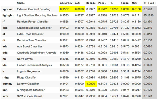
Figure 6.
ML models performance comparison for defect prediction.
All metrics (accuracy, AUC, recall, precision, F1, kappa, MCC, and inference time) are computed on the test data after cross-validated training. Although tabular in format, the figure is retained for consistency with the graphical outputs generated in Python 3.10.
Based on the comparative results, XGBoost was selected as the best-performing algorithm, despite its black-box nature. As such, ensuring interpretability is relevant to understanding the decision-making process behind defect classification. Prior to applying explainability techniques, we fine-tuned the model’s hyperparameters to optimize performance and mitigate class imbalance, as the distribution of defective versus non-defective samples is skewed. This imbalance is illustrated in Figure 7.
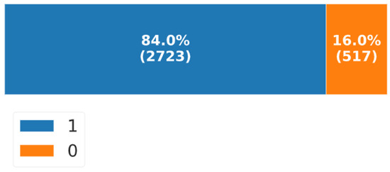
Figure 7.
Manufacturing defects (1 = yes; 0 = no).
Following the hyperparameter optimization and class balancing procedures, the final XGBoost model demonstrated high predictive performance. The model was fine-tuned using a focused grid search strategy, and the final hyperparameter configuration included n_estimators = 150, max_depth = 6, learning_rate = 0.10, subsample = 0.85, colsample_bytree = 0.75, gamma = 0.5, reg_alpha = 0.3, and reg_lambda = 1.2. These values were selected based on cross-validation performance prior to final testing.
As shown in Figure 8, the confusion matrix reveals a strong capability to distinguish between defective and non-defective products. The model correctly classified 678 out of 681 defective samples (true positives), while misclassifying only 3 (false negatives). For non-defective cases, 101 were correctly predicted (true negatives), with 28 misclassified as defective (false positives). This corresponds to a high recall for the minority class (recall = 0.9956), strong overall accuracy (accuracy = 0.9629), and excellent F1-score (F1 = 0.9776), confirming the model’s capacity to generalize effectively beyond the training data.
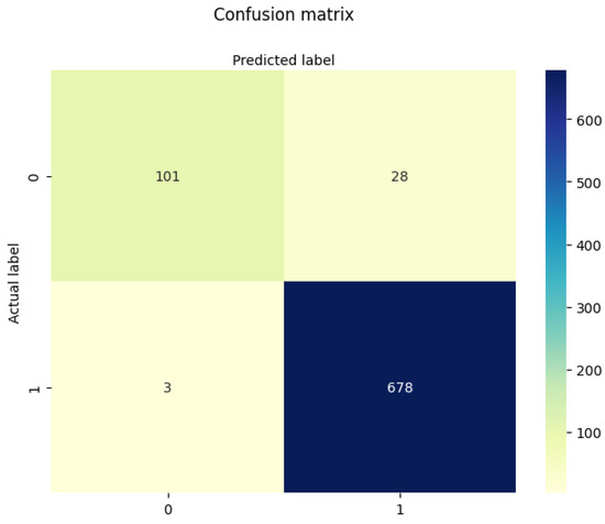
Figure 8.
Evaluation of XGBoost predictions with balanced data.
From an operational standpoint, the classifier adopts a conservative bias toward defect detection, prioritizing recall over precision (precision = 0.9603), which is often desirable in high-risk manufacturing settings, where missing a defective product (false negative) is more critical than over-inspecting a non-defective one (false positive). Most false positives occur in borderline cases, where high values of “MaintenanceHours” or “DefectRate” coincide with moderate “QualityScore”, suggesting the need for richer contextual features (e.g., operator data, sensor logs) to further reduce ambiguity.
4.1.3. Interpretability
This section presents the results obtained using five prominent XAI techniques, SHAP, LIME, ELI5, PDP, and ICE, applied to the trained XGBoost model. These techniques offer complementary perspectives that enhance the model’s interpretability and contribute to a more robust understanding of the underlying process conditions leading to defects.
SHAP
To gain a comprehensive understanding of how the XGBoost model differentiates between defective and non-defective products, SHAP summary plots were generated for both class 1 (defective) and class 0 (non-defective) predictions.
As shown in Figure 9, the most influential features are consistent across both classes, “MaintenanceHours”, “DefectRate”, “QualityScore”, and “ProductionVolume”.
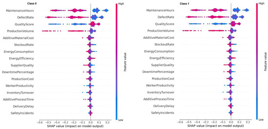
Figure 9.
SHAP value distribution for class 0 and class 1.
For class 1 (defective products), higher values of “MaintenanceHours” and “DefectRate” are associated with large positive SHAP values, indicating a strong contribution to the likelihood of defects. In contrast, higher values of “QualityScore” display negative SHAP values, suggesting a protective effect by decreasing the predicted probability of defect.
For class 0 (non-defective products), the pattern is symmetrical, as lower “MaintenanceHours” and “DefectRate”, combined with higher “QualityScore”, contribute to lower defect probabilities. The SHAP distributions for class 0 are more centered around zero and exhibit lower variance, indicating that the model confidently identifies non-defective products under more stable and predictable conditions.
This symmetry in feature contributions between classes confirms the internal consistency of the model and highlights “QualityScore” as a key differentiator with a negative impact on defect classification.
LIME
LIME was used to generate local explanations for two instances as follows:
- Product 0 classified as defective with a predicted probability of 0.95.
- Product 200 classified as non-defective with a predicted probability of 0.93.
As shown in Figure 10, LIME produces a ranked list of feature contributions for each individual prediction, based on local linear approximations of the XGBoost model.
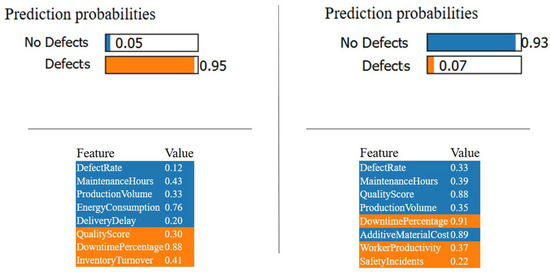
Figure 10.
LIME explanations for two individual predictions.
In the defective case (left panel), the most influential features increasing the defect probability are the following:
- “DowntimePercentage” = 0.88, with a strong positive contribution.
- “InventoryTurnover” = 0.41, and “MaintenanceHours” = 0.43, both with moderate effects.
- In contrast, “DefectRate” = 0.12 and “QualityScore” = 0.30 appear to have slightly negative contributions, suggesting a minor mitigating effect on the prediction.
In the non-defective case (right panel), the main contributors to the low predicted defect probability include the following:
- “QualityScore” = 0.88, showing a strong negative contribution (protective),
- “WorkerProductivity” = 0.37, and
- “AdditiveMaterialCost” = 0.89, both supporting the non-defect classification.
An interesting insight is the presence of “DowntimePercentage” as a high value (0.91) in this second case as well. However, in this context, it contributes negatively to the probability of defect, illustrating LIME’s local nature and how the effect of a variable can shift depending on the surrounding feature values.
This analysis confirms that LIME complements global interpretability techniques (e.g., SHAP) by providing instance-specific explanations, reflecting subtle interactions that drive classification decisions on a local scale.
ELI5
To extract a global ranking of feature importance from the trained XGBoost model, we employed ELI5, which provides an interpretable weight for each variable based on its contribution across all decision trees. These weights reflect the average impact of each feature on model predictions, along with their associated standard deviations.
As shown in Figure 11, the top five most influential features identified by ELI5 are “MaintenanceHours”, “DefectRate”, “QualityScore”, “ProductionVolume”, and “AdditiveMaterialCost”.
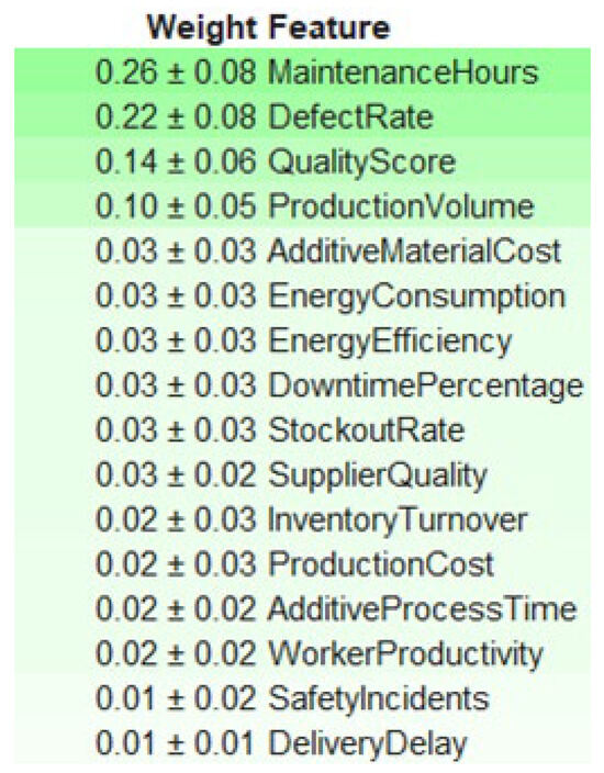
Figure 11.
Feature importance weights obtained from ELI5.
This ranking aligns with the results obtained from SHAP and LIME analyses, particularly reinforcing the importance of “MaintenanceHours”, “DefectRate”, and “QualityScore” as critical predictors of defective outputs. The relatively low importance of variables, such as “DeliveryDelay”, “SafetyIncidents”, and “WorkerProductivity”, suggests a minor role in the model’s global decision logic.
Moreover, the consistency between the rankings derived from ELI5 and other explainability techniques enhances the trustworthiness of the model, indicating a stable internal structure and confirming that its most decisive variables are also those most interpretable and actionable from a quality management perspective.
PDP and ICE
To further understand the marginal effects of specific features on the model’s output, we employed Partial Dependence Plots (PDP) combined with Individual Conditional Expectation (ICE). These techniques visualize how variations in each feature affect the predicted probability of defects, both on average (PDP) and across individual instances (ICE).
Figure 12 and Figure 13 show the joint PDP–ICE curves for the two most influential variables, “MaintenanceHours” and “DefectRate”.
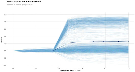
Figure 12.
PDP for “MaintenanceHours” feature.
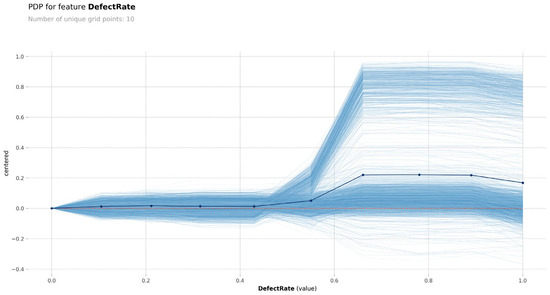
Figure 13.
PDP for “DefectRate” feature.
- For “MaintenanceHours”, there is a clear positive non-linear relationship; once the normalized value exceeds ~0.4, the predicted probability of defect increases steeply. The ICE curves confirm this trend across nearly all instances, indicating consistent model behavior.
- Similarly, for “DefectRate”, low values are associated with low predicted risk, but from ~0.6 onwards, the model output rises rapidly. The ICE variability slightly increases for higher defect rates, suggesting greater sensitivity in that range.
These visualizations provide model-agnostic evidence of the monotonic influence of these two variables, supporting the findings from SHAP, ELI5, and feature importance rankings. The combination of PDP and ICE thus reinforces the reliability and interpretability of the model’s behavior regarding these key predictors.
4.2. Fuzzy Clustering and Profile Interpretation
In this section, we report the outcomes of the Fuzzy C-Means (FCM) clustering applied to the production features, excluding the “DefectStatus” target label, to maintain a purely unsupervised perspective. This segmentation aims to uncover latent operational profiles within the dataset, potentially associated with quality-relevant process behaviors.
The resulting clusters are subsequently interpreted using the same Explainable AI (XAI) methods employed in the supervised track, enabling the identification of dominant variables within each group and allowing a consistent interpretability layer across both modeling approaches. Finally, the discovered cluster profiles are compared against the predicted defect probabilities, supporting a structural coherence analysis between unsupervised groupings and supervised classifications. The choice of FCM is motivated by its ability to model partial membership, which reflects the inherent ambiguity in real-world production processes. Rather than increasing system complexity, fuzzy clustering enhances interpretability by capturing gradual transitions and overlapping defect characteristics.
4.2.1. Cluster Optimization Using Silhouette Index
Before applying the Fuzzy C-Means (FCM) algorithm, we performed a preliminary analysis to determine the optimal number of clusters (c). The “DefectStatus” variable was excluded from this step to ensure a purely unsupervised perspective. All numerical features were normalized using Min-Max scaling to the range [0, 1], to prevent scale dominance in the clustering process.
To identify the best clustering configuration, we evaluated values of c from 2 to 10 using the Silhouette Index, a standard metric that quantifies the degree of cohesion within clusters and separation between them. For each c, the silhouette score was computed from the hard partitioning derived via a crisp K-means approximation of the fuzzy memberships.
This index was selected over other alternatives (e.g., Calinski–Harabasz, Davies–Bouldin) due to its robustness and interpretability, especially in normalized, low-dimensional settings like the present one. Unlike metrics that may favor excessive partitioning or require strong distributional assumptions, the silhouette score offers a more intuitive and balanced measure of cluster structure, facilitating clearer decision-making in unsupervised analysis.
The optimal number of clusters was selected as the one yielding the highest silhouette score, ensuring a balance between intra-cluster compactness and inter-cluster separability. As shown in Figure 14, the maximum silhouette value occurs at , suggesting that the data is best structured around two main production profiles.
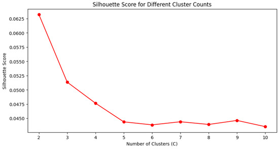
Figure 14.
Silhouette Index values for different numbers of clusters.
This two-cluster configuration will serve as the foundation for the FCM clustering stage, enabling interpretability through soft membership degrees rather than binary assignments, and setting the stage for subsequent structural analysis with XAI.
4.2.2. Fuzzy Partitioning and Cluster Profile Analysis
The FCM algorithm yielded a membership matrix that assigns each observation a soft degree of belonging to each cluster. A hard label was then derived by assigning each point to the cluster with the highest membership score, allowing comparison with classification outcomes.
To interpret the resulting clusters, we analyzed the centroids derived from the fuzzy partitioning. However, as illustrated in Figure 15 and Figure 16, the profiles of both clusters were nearly identical, with minimal variation across features. This limited contrast suggests that the fuzzy segmentation did not capture meaningful operational heterogeneity. The lack of distinct cluster identity may be attributed to the absence of strong latent structure within the data when viewed through the lens of Euclidean distance and linear relationships.
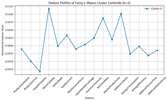
Figure 15.
Feature profiles for Cluster 0.
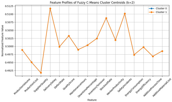
Figure 16.
Feature profiles for Cluster 1.
To validate this observation, we also explored the distribution of the “DefectStatus” variable within each cluster, Figure 17. The results showed that both clusters contained similar proportions of defective and non-defective samples, reinforcing the conclusion that defect-related structure is not inherently discoverable through unsupervised clustering alone.
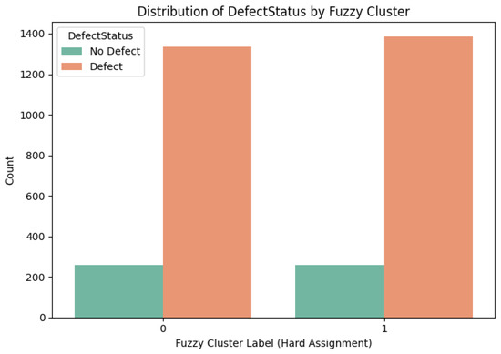
Figure 17.
Distribution of the “DefectStatus” variable within each cluster.
This outcome contrasts with the high performance of the supervised XGBoost model discussed in Section 4.1, which successfully identified defective instances with strong accuracy. The model captured complex, non-linear interactions between features that were invisible to clustering methods, such as the combined effect of “MaintenanceHours”, “DefectRate”, and “QualityScore”. This highlights the advantage of supervised learning supported by explainability tools in uncovering hidden quality patterns in industrial data.
These findings are consistent with previous studies noting that clustering algorithms such as FCM or K-means often struggle to identify meaningful patterns when the data lacks well-separated or linearly separable substructures, particularly in industrial environments characterized by high-dimensional noise and intertwined variables [40,41]. As argued in [42], in such contexts, supervised models enhanced with explainable AI offer a more effective and interpretable approach to pattern detection and decision support.
Nevertheless, FCM provides a valuable framework for soft segmentation, and its combination with explainable AI in subsequent steps enables the extraction of latent process insights that transcend the limitations of traditional clustering techniques.
4.2.3. Clustering Based on K-Means (k = 3)
As a complementary approach to the fuzzy clustering strategy, we applied the classic K-means algorithm to analyze the latent structure of the manufacturing dataset using a hard partition into three clusters.
We selected the same input features used in the fuzzy model, excluding the target variable “DefectStatus”. The data were standardized using z-score normalization, and the K-means algorithm was applied with k = 3 and n_init = 10 to improve solution stability. The resulting cluster assignments were then added to the dataset under the column Cluster_KMeans.
The distribution of samples across the three clusters was relatively balanced:
- Cluster 0: 1066 samples
- Cluster 1: 1057 samples
- Cluster 2: 1117 samples
To better understand the internal structure of each cluster, we computed the centroids in both the original and normalized variable spaces. The normalized version (based on z-scores) was used for visualization, enabling comparison across features with very different ranges and variances.
PCA visualization, Figure 18, reveals a continuous spread of the data with partial overlaps between clusters, consistent with the low Silhouette Score obtained (~0.056). This indicates that while the clusters are not strongly separated in geometric terms, the K-means algorithm is still capable of capturing underlying patterns in the data.
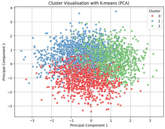
Figure 18.
Cluster visualization with K-means (PCA).
To provide a clearer understanding of the cluster profiles, we created a grouped bar chart showing the normalized centroids per feature and per cluster, Figure 19. This visualization highlights variable-specific differences between clusters.
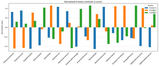
Figure 19.
Normalized K-means centroids (z-score).
Key differences observed among the K-means clusters are as follows:
- Cluster 0 exhibits high values in “WorkerProductivity” and “QualityScore”, along with low “StockoutRate”. This profile suggests an efficient and stable production environment, likely characterized by effective resource utilization and fewer supply-related disruptions.
- Cluster 1 is defined by the highest levels of “DefectRate”, “SafetyIncidents”, and “EnergyConsumption”. These patterns indicate operational inefficiencies and potential safety risks, pointing to a high-risk and resource-intensive segment.
- Cluster 2 displays a more balanced configuration, with above-average “EnergyEfficiency” and low “DefectRate”. These traits are indicative of a sustainable and quality-oriented production profile, potentially driven by well-calibrated processes and controlled inputs.
These results support several conclusions:
- K-means can reveal meaningful operational distinctions even in high-dimensional manufacturing datasets, especially when aided by post hoc interpretability tools.
- The identified clusters provide a foundation for intermediate labeling, which can be further exploited in supervised tasks such as quality forecasting or process optimization.
- Compared with the FCM results (Section 4.2.2), K-means clustering demonstrates greater internal contrast and operational differentiation, making it a more informative tool for segment-based analysis in this case.
4.2.4. Cluster Membership Prediction with XGBoost and Explainable AI
To further explore the interpretability of the clusters obtained via K-means, we trained a supervised classifier with the objective of predicting cluster membership based on the original feature set. This strategy allows us to assess whether the clustering structure is recoverable and explainable from the input data, and to evaluate which variables are most influential in distinguishing between groups.
The methodology followed involved the following steps. First, the Cluster_KMeans labels obtained from the unsupervised K-means process (with k = 3) were used as the target variable for a supervised classification task.
XGBoost
An XGBoost classifier was then trained using the same set of standardized features previously used in the clustering phase. The dataset was split into training and test subsets using an 80/20 ratio to evaluate generalization performance. To enhance model robustness, a manual fine-tuning of the XGBoost hyperparameters was conducted. The final configuration used the following settings: n_estimators = 120, max_depth = 4, learning_rate = 0.15, subsample = 0.9, colsample_bytree = 0.8, gamma = 1.0, reg_alpha = 0.2, and reg_lambda = 0.8. These values were selected through targeted experimentation based on validation performance and were fixed prior to final model evaluation.
The model achieved high classification accuracy, as illustrated in Figure 20, where the confusion matrix shows a strong correspondence between predicted and actual cluster labels, with most instances correctly assigned to their respective groups.
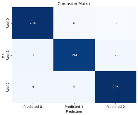
Figure 20.
Confusion matrix, membership of each cluster.
The classifier correctly predicted 204, 194, and 205 samples for classes 0, 1, and 2, respectively, resulting in an overall accuracy of 92.90%. Class-wise analysis reveals strong performance across all categories, with macro-averaged precision of 0.9308, recall of 0.9307, and F1-score of 0.9304, indicating excellent balance and robustness.
The highest recall was achieved for class 0 (0.9577), while class 2 showed the best precision (0.9535), reflecting the model’s ability to discriminate subtle variations in defect profiles. Most misclassifications involve confusion between classes 1 and 2, particularly in borderline cases where a high “DefectRate” and “MaintenanceHours” coincide with moderate values of “QualityScore” or other overlapping signals.
These findings suggest a potential gain from incorporating additional operational features (e.g., shift patterns, sensor anomalies, operator logs) to refine class separation and further reduce ambiguity in future iterations.
Global Explainability (SHAP)
To understand the general behavior of the model, we applied SHAP to estimate the mean contribution of each feature to the model output:
We analyzed SHAP values separately by cluster, as shown in Figure 21.
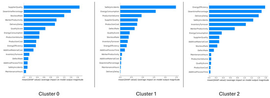
Figure 21.
SHAP values by cluster.
Cluster 0 is defined by high “SupplierQuality”, low “DowntimePercentage”, and low “StockoutRate”, aligning with its centroid traits of high “WorkerProductivity” and “QualityScore”. Altogether, these results indicate a highly efficient and stable production environment with minimal disruptions and reliable inputs.
Cluster 1 is predominantly influenced by high “SafetyIncidents”, “EnergyConsumption”, and “ProductionVolume”. These findings are fully aligned with the centroid profile, which also revealed elevated “DefectRate” and operational inefficiencies. Together, these indicators point to a risk-prone and resource-intensive cluster, potentially affected by lower safety standards and suboptimal process control.
Cluster 2 is mainly characterized by high “EnergyEfficiency”, along with low “DowntimePercentage” and “SafetyIncidents”. These patterns confirm the centroid-based interpretation, where this cluster displayed a balanced operational profile with above-average “EnergyEfficiency” and low “DefectRate”. Overall, Cluster 2 reflects a sustainable and quality-oriented production segment, likely to benefit from well-controlled processes and minimal disruptions.
Local Explainability (LIME)
To complement the global perspective, we applied LIME to individual instances, one from each cluster, offering a fine-grained view of the decision logic behind each prediction, as shown in Figure 22.
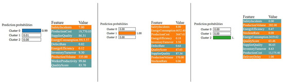
Figure 22.
LIME explanations for three individual predictions.
For the analyzed instance classified into Cluster 0, LIME confirms the dominance of features such as high “SupplierQuality”, “WorkerProductivity”, and “QualityScore”, in line with the global SHAP interpretation and centroid analysis. Despite the presence of some values typically associated with Cluster 1 (e.g., “EnergyConsumption”, “SafetyIncidents”), the model assigns the instance to Cluster 0 with high confidence (0.99), reinforcing its identity as a stable and efficient production profile.
For the analyzed instance assigned to Cluster 1, LIME highlights the contribution of high “SafetyIncidents”, “EnergyConsumption”, and low “EnergyEfficiency”, which align closely with the global SHAP findings and centroid-based profile. The model assigns this instance to Cluster 1 with full confidence (1.00), characterizing it as a risk-prone and resource-intensive case, reflective of potential safety concerns and operational inefficiencies.
For the analyzed instance classified into Cluster 2, LIME highlights the impact of high “EnergyEfficiency” and low “SafetyIncidents” as key factors supporting the model’s prediction. The instance also shows moderate “ProductionVolume” and low “StockoutRate”, which further reinforce the assignment. With a prediction probability of 1.00, this case is clearly associated with Cluster 2’s sustainable and balanced production profile, characterized by efficient resource usage and process stability.
4.3. Summary and Final Remarks
The experimental analysis presented in this section has combined supervised learning, unsupervised clustering, and explainable AI to uncover patterns, predict outcomes, and interpret operational behaviors in manufacturing environments. The dual modeling framework proposed, comprising defect prediction and process segmentation, has demonstrated high predictive capacity, structural coherence, and interpretability.
In the first part (Section 4.1), a supervised approach was applied to predict defect occurrence using several machine learning models. After comparative evaluation, the XGBoost classifier emerged as the most effective, achieving 95.37% accuracy, high recall for the minority class, and strong generalization. The use of SHAP, LIME, ELI5, PDP, and ICE enabled a detailed understanding of the internal decision logic, consistently identifying “MaintenanceHours”, “DefectRate”, and “QualityScore” as critical drivers of defect classification. Local explanations further highlighted context-dependent feature interactions, reinforcing the model’s transparency and trustworthiness.
In the second part (Section 4.2), unsupervised clustering methods were employed to segment production profiles. While the initial Fuzzy C-Means (FCM) analysis revealed limited separation and no clear alignment with defect labels, the alternative application of K-means clustering (k = 3) provided more interpretable and operationally meaningful groupings. Each cluster was associated with a distinct set of characteristics:
- Cluster 0: high efficiency and quality, with high “WorkerProductivity” and “SupplierQuality”, and low “StockoutRate”.
- Cluster 1: marked by inefficiency and risk, with high “SafetyIncidents”, “DefectRate”, and “EnergyConsumption”.
- Cluster 2: balanced and sustainable, with above-average “EnergyEfficiency” and low “DowntimePercentage”.
To test the internal validity of the cluster structure, a new XGBoost model was trained to classify observations by cluster membership. The classifier achieved high accuracy, and SHAP confirmed that the most relevant features for each cluster aligned with those identified by K-means centroids. LIME explanations of individual instances further corroborated the semantic coherence of each profile.
Overall, the results demonstrate the strength of combining predictive modeling, unsupervised learning, and explainable AI to develop interpretable frameworks for manufacturing quality analysis. Although a full mathematical benchmarking of explainability methods was initially planned, we leave its formalization and quantification (e.g., entropy, stability, and ranking convergence) for future work. Nevertheless, the consistency across global (SHAP), local (LIME), and structural (clustering) interpretations provides a strong basis for human-in-the-loop decision-making and quality assurance in industrial contexts.
5. Discussion and Future Works
5.1. Supervised Defect Prediction and Explainability
In regulated industrial environments, such as those operating under ISO 9001 or FDA guidelines, model transparency is not merely desirable but essential. Explainability ensures traceability in decision-making, supports audit readiness, and fosters operator trust, key aspects for AI adoption in quality-critical domains.
The first part of our framework focused on the supervised classification of defective products using the XGBoost algorithm. The model consistently outperformed all other classifiers tested (Figure 6), achieving a remarkable accuracy of 95.37% with an AUC of 0.8826, recall of 0.9927, and a balanced precision (0.9542) and F1-score (0.9730). These values suggest not only high discriminative power, but also robustness in handling the class imbalance present in the dataset.
The confusion matrix further highlights the model’s reliability; out of 681 defective items, only 3 were misclassified, and most non-defective samples were correctly labeled, as shown in Figure 8. This outcome is particularly relevant in quality control contexts, where minimizing false negatives is critical for operational safety and customer satisfaction.
Interpretation techniques were key to interpreting these results. For SHAP values, Figure 9 shows that “MaintenanceHours”, “DefectRate”, and “QualityScore” were the most influential features. “MaintenanceHours” and “DefectRate” made strong positive contributions to the defective class, aligning with domain expectations. Conversely, higher “QualityScore” values reduced the likelihood of being classified as defective, confirming its protective effect.
These global insights were validated locally using LIME, which offered case-specific justifications, Figure 10. The two analyzed instances illustrated the contrast between defect and non-defect predictions, reaffirming the importance of process conditions like “DowntimePercentage”, “InventoryTurnover”, and “QualityScore” in shaping the classification decision.
Furthermore, ELI5 rankings, Figure 11, reinforced the SHAP conclusions, confirming the central role of “MaintenanceHours” and “DefectRate”. PDP and ICE visualizations (Figure 12 and Figure 13) complemented these findings by demonstrating monotonic and non-linear effects of these predictors. For instance, the sharp increase in defect probability when “MaintenanceHours” exceeded a normalized threshold of ~0.4 suggested a critical operational tipping point.
5.2. Clustering-Based Segmentation and Interpretability
In the second part of the framework, we explored the unsupervised structure of the dataset through two clustering strategies: Fuzzy C-Means (FCM) and K-means, aiming to uncover latent operational profiles beyond the defect classification task. While FCM revealed limited internal contrast between segments, the K-means model (with k = 3) produced interpretable groupings aligned with plausible manufacturing configurations.
The centroid profiles obtained through K-means (Figure 19) revealed clear differentiating patterns.
Cluster 0 was associated with high “WorkerProductivity” and “QualityScore”, and low “StockoutRate”, suggesting a highly efficient and stable production environment.
Cluster 1, on the contrary, exhibited high “DefectRate”, “SafetyIncidents”, and “EnergyConsumption”, indicating a risk-prone, resource-intensive configuration with potential process inefficiencies.
Cluster 2 represented a balanced segment with elevated “EnergyEfficiency” and low “DowntimePercentage”, reflecting a sustainable, quality-oriented profile.
These operational identities were validated through a supervised XGBoost classifier trained to predict K-means cluster labels. The high classification accuracy (Figure 20) confirmed the recoverability of the cluster structure from the input variables. Moreover, the use of SHAP values (Figure 21) allowed us to identify the main drivers for each group as follows:
- Cluster 0: most influenced by “SupplierQuality”, “DowntimePercentage”, and “StockoutRate”, consistent with a lean and input-stable process.
- Cluster 1: dominated by “SafetyIncidents”, “EnergyConsumption”, and “ProductionVolume”, reflecting stress in production intensity and safety protocols.
- Cluster 2: defined by “EnergyEfficiency”, “DowntimePercentage”, and “SafetyIncidents”, capturing a scenario of optimized and controlled operations.
The LIME explanations (Figure 22) for individual predictions further reinforced these patterns. For each analyzed instance, LIME confirmed that the features driving the local decisions were in alignment with the global SHAP profiles and centroid characteristics.
These results provide empirical support for the coherence and consistency between unsupervised segmentation and model-based explainability. Even though clustering operates independently of the target variable, the emerging groupings showed meaningful alignment with the patterns observed in the defect prediction task. Cluster 1 overlaps substantially with the high-defect regions, while Clusters 0 and 2 appear more aligned with efficient and defect-minimizing behaviors.
Therefore, the dual approach incorporated in this study helps us to determine actionable subpopulations within the production environment, as well as ensuring interpretability and reliability through complementary XAI techniques. This knowledge can serve as a basis for specific interventions, such as preventive maintenance, supplier quality assessment or energy optimization.
5.3. Future Work
Several avenues for extension and generalization emerge from this study:
- Integration of temporal data: incorporating time series from production lines could enhance both prediction and segmentation capabilities, enabling dynamic monitoring of quality drifts and transitions between operational states.
- Hybrid clustering approaches: combining fuzzy logic with supervised guidance, such as semi-supervised learning or constrained FCM, may improve cluster separability while preserving the benefits of soft membership.
- Multimodal data fusion: enriching the model with additional modalities such as maintenance logs (text), product images, or real-time sensor data could support a more comprehensive and context-aware pipeline.
- Prescriptive analytics: moving beyond prediction, the identified clusters and explainability outputs could inform prescriptive actions, such as maintenance scheduling, energy optimization, or quality assurance policies.
- Deployment in real-time environments: validating the framework within streaming architectures or digital twin systems would help test its scalability, responsiveness, and operational feasibility in real-world settings.
- Implementation of the proposed XAI evaluation framework: while Section 3.4 introduces a mathematically grounded evaluation structure for explainability methods, its full implementation remains open. Applying these formal metrics will allow robust benchmarking of interpretability, fidelity, and stability across techniques.
Ultimately, this work proposes a generalizable methodology for analyzing complex manufacturing systems by integrating high-performance prediction, soft clustering, and explainable AI. This hybrid approach supports both operational insight and actionable decision-making, core requirements for intelligent, transparent, and adaptive Industry 4.0 systems.
5.4. Limitations
While the proposed framework demonstrated strong predictive performance, interpretability, and structural coherence, several limitations must be acknowledged:
- Synthetic nature of the dataset: although the dataset is grounded in empirical industrial distributions and reflects realistic operational dynamics, it remains synthetic. Consequently, the generalizability of results to specific industrial environments should be validated with real-world production data.
- Clustering assumptions and structure: the Fuzzy C-Means algorithm assumes spherical geometry and Euclidean distance, which may not be well-suited for capturing non-linear or intertwined relationships between process variables. This limitation became evident in the minimal separation between clusters, especially when compared to the supervised results.
- Absence of temporal or sequential data: the current approach is based on static observations. In real manufacturing systems, quality deviations often emerge over time. The integration of temporal data streams or event logs would enable more dynamic and context-aware predictions.
- Interpretability remains qualitative: while a mathematical framework for evaluating explainability was proposed, the actual application of quantitative metrics (e.g., attribution entropy, ranking consistency, fidelity scores) remains a subject for future work. At present, the interpretability analysis relies on visual coherence across XAI techniques (SHAP, LIME, etc.), which though informative, is inherently subjective.
These limitations open opportunities for future research, particularly in extending the methodology to real-time environments, being validated with industrial datasets, and implementing the formal evaluation layer introduced in Section 3.4.
6. Conclusions
We proposed and validated a dual modeling framework that integrates supervised learning, unsupervised clustering, and Explainable AI (XAI) to support quality control and operational profiling in manufacturing environments.
In the first phase, we focused on defect prediction using the XGBoost algorithm. The model achieved high performance (accuracy = 95.37%, recall = 99.27%) and demonstrated strong generalization. The application of five post hoc XAI techniques (SHAP, LIME, ELI5, PDP, and ICE) enabled transparent interpretation of the decision logic. Key features “MaintenanceHours”, “DefectRate”, and “QualityScore” consistently emerged as the most influential, aligning with expert knowledge and validating the model’s interpretability.
In the second phase, unsupervised clustering was applied to the same input space. While Fuzzy C-Means offered limited structural separation, K-means (k = 3) revealed three meaningful clusters as follows: (i) efficient and high-quality (Cluster 0), (ii) risk-prone and resource-intensive (Cluster 1), and (iii) balanced and sustainable (Cluster 2).
To validate consistency, we trained an XGBoost model to predict cluster assignments. The classifier performed strongly, and SHAP and LIME analyses confirmed that the variables distinguishing clusters overlapped with those used in defect prediction. This semantic coherence was further reinforced through convergence across global (SHAP), local (LIME), and structural (centroid) interpretations.
A final cross-methodological analysis confirmed that features such as “DefectRate”, “EnergyEfficiency”, “SafetyIncidents”, and “QualityScore” play an important role in both modeling tracks. Their consistent relevance underscores the internal alignment of the framework.
Although we have proposed a formal mathematical framework for XAI evaluation (Section 3.4), its quantitative implementation remains as future work. Completing this layer would further strengthen the robustness and theoretical soundness of interpretable AI in industrial applications.
Overall, the results demonstrate that the combination of supervised prediction, unsupervised clustering, and XAI provides a robust, interpretable, and actionable methodology for manufacturing analysis. This hybrid framework supports both operational insight and strategic intervention, contributing to the development of intelligent, transparent, and adaptive systems aligned with Industry 4.0 principles.
Future research will extend this framework to real-time systems, multimodal data (e.g., logs, sensors, and images), and prescriptive analytics to build resilient, explainable solutions for complex production environments.
Funding
This research received no external funding.
Data Availability Statement
The data source can be accessed via the following link: https://www.kaggle.com/datasets/rabieelkharoua/predicting-manufacturing-defects-dataset. (accessed on 2 May 2025).
Conflicts of Interest
The authors declare no conflicts of interest.
References
- ISO 9001:2015; Quality Management Systems—Requirements. International Organization for Standardization: Geneva, Switzerland, 2015.
- Bousdekis, A.; Lepenioti, K.; Apostolou, D.; Mentzas, G. Data analytics in quality 4.0: Literature review and future research directions. Int. J. Comput. Integr. Manuf. 2023, 36, 678–701. [Google Scholar] [CrossRef]
- Saberironaghi, A.; Ren, J.; El-Gindy, M. Defect Detection Methods for Industrial Products Using Deep Learning Techniques: A Review. Algorithms 2023, 16, 95. [Google Scholar] [CrossRef]
- Molnar, C. Interpretable Machine Learning. A Guide for Making Black Box Models Explainable. Book. p. 247. 2019. Available online: https://christophm.github.io/interpretable-ml-book (accessed on 19 May 2025).
- Marín Díaz, G.; Hernández, J.J.G. Decoding Employee Attrition: A Unified Approach with XAI and AHP. In Intelligent Management of Data and Information in Decision Making; World Scientific Publishing Co Pte Ltd.: Singapore, 2024; pp. 367–375. [Google Scholar]
- Metta, C.; Beretta, A.; Pellungrini, R.; Rinzivillo, S.; Giannotti, F. Towards Transparent Healthcare: Advancing Local Explanation Methods in Explainable Artificial Intelligence. Bioengineering 2024, 11, 369. [Google Scholar] [CrossRef]
- Abdul, A.; Vermeulen, J.; Wang, D.; Lim, B.Y.; Kankanhalli, M. Trends and trajectories for explainable, accountable and intelligible systems: An HCI research agenda. In Proceedings of the 2018 CHI Conference on Human Factors in Computing Systems, Montreal, QC, Canada, 21–26 April 2018; Volume 2018. [Google Scholar] [CrossRef]
- Marín Díaz, G.; Galán Hernández, J.J.; Galdón Salvador, J.L. Analyzing Employee Attrition Using Explainable AI for Strategic HR Decision-Making. Mathematics 2023, 11, 2023. [Google Scholar] [CrossRef]
- Kharoua, R. El Predicting Manufacturing Defects Dataset. Kaggle. 2023. Available online: https://www.kaggle.com/datasets/rabieelkharoua/predicting-manufacturing-defects-dataset (accessed on 19 May 2025).
- Marín Díaz, G. Quality Management in Chemical Processes Through Fuzzy Analysis: A Fuzzy C-Means and Predictive Models Approach. ChemEngineering 2025, 9, 45. [Google Scholar] [CrossRef]
- Marín Díaz, G.; Gómez Medina, R.; Aijón Jiménez, J.A. A Methodological Framework for Business Decisions with Explainable AI and the Analytic Hierarchical Process. Processes 2025, 13, 102. [Google Scholar] [CrossRef]
- Marín Díaz, G.; Gómez Medina, R.; Aijón Jiménez, J.A. Integrating Fuzzy C-Means Clustering and Explainable AI for Robust Galaxy Classification. Mathematics 2024, 12, 2797. [Google Scholar] [CrossRef]
- Yang, J.; Li, S.; Wang, Z.; Dong, H.; Wang, J.; Tang, S. Using deep learning to detect defects in manufacturing: A comprehensive survey and current challenges. Materials 2020, 13, 5755. [Google Scholar] [CrossRef]
- Rodriguez-Fernandez, V.; Camacho, D. Recent trends and advances in machine learning challenges and applications for industry 4.0. Expert Syst. 2024, 41, e13506. [Google Scholar] [CrossRef]
- Iqbal, R.; Maniak, T.; Doctor, F.; Karyotis, C. Fault Detection and Isolation in Industrial Processes Using Deep Learning Approaches. IEEE Trans. Ind. Inform. 2019, 15, 3077–3084. [Google Scholar] [CrossRef]
- Saufi, S.R.; Ahmad, Z.A.B.; Leong, M.S.; Lim, M.H. Challenges and opportunities of deep learning models for machinery fault detection and diagnosis: A review. IEEE Access 2019, 7, 122644–122662. [Google Scholar] [CrossRef]
- Loh, C.H.; Chen, Y.C.; Su, C.T. Using Transfer Learning and Radial Basis Function Deep Neural Network Feature Extraction to Upgrade Existing Product Fault Detection Systems for Industry 4.0: A Case Study of a Spring Factory. Appl. Sci. 2024, 14, 2913. [Google Scholar] [CrossRef]
- Choi, K.; Yi, J.; Park, C.; Yoon, S. Deep Learning for Anomaly Detection in Time-Series Data: Review, Analysis, and Guidelines. IEEE Access 2021, 9, 120043–120065. [Google Scholar] [CrossRef]
- Aboulhosn, Z.; Musamih, A.; Salah, K.; Jayaraman, R.; Omar, M.; Aung, Z. Detection of Manufacturing Defects in Steel Using Deep Learning With Explainable Artificial Intelligence. IEEE Access 2024, 12, 99240–99257. [Google Scholar] [CrossRef]
- Rožanec, J.M.; Novalija, I.; Zajec, P.; Kenda, K.; Tavakoli Ghinani, H.; Suh, S.; Veliou, E.; Papamartzivanos, D.; Giannetsos, T.; Menesidou, S.A.; et al. Human-centric artificial intelligence architecture for industry 5.0 applications. Int. J. Prod. Res. 2022, 61, 6847–6872. [Google Scholar] [CrossRef]
- Yoo, S. Explainable Artificial Intelligence for Manufacturing Cost Estimation and Machining Feature Visualization. Expert Syst. Appl. 2021, 183, 115430. [Google Scholar] [CrossRef]
- Mishra, A.; Jatti, V.S.; Sefene, E.M.; Paliwal, S. Explainable Artificial Intelligence (XAI) and Supervised Machine Learning-based Algorithms for Prediction of Surface Roughness of Additively Manufactured Polylactic Acid (PLA) Specimens. Appl. Mech. 2023, 4, 668–698. [Google Scholar] [CrossRef]
- Ukwaththa, J.; Herath, S.; Meddage, D.P.P. A review of machine learning (ML) and explainable artificial intelligence (XAI) methods in additive manufacturing (3D Printing). Mater. Today Commun. 2024, 41. [Google Scholar] [CrossRef]
- Bezdek, J.C.; Ehrlich, R.; Full, W. FCM: The fuzzy c-means clustering algorithm. Comput. Geosci. 1984, 10, 191–203. [Google Scholar] [CrossRef]
- Gindy, N.N.Z.; Ratchev, T.M.; Case, K. Component grouping for GT applications—A fuzzy clustering approach with validity measure. Int. J. Prod. Res. 1995, 33, 2493–2509. [Google Scholar] [CrossRef]
- Abdulshahed, A.M.; Longstaff, A.P.; Fletcher, S.; Myers, A. Thermal error modelling of machine tools based on ANFIS with fuzzy c-means clustering using a thermal imaging camera. Appl. Math. Model. 2015, 39, 1837–1852. [Google Scholar] [CrossRef]
- Zanoli, S.M.; Pepe, C. Design and Implementation of a Fuzzy Classifier for FDI Applied to Industrial Machinery. Sensors 2023, 23, 6954. [Google Scholar] [CrossRef]
- Yang, J.; Su, J.; Song, L. Selection of manufacturing enterprise innovation design project based on consumer’s green preferences. Sustainability 2019, 11, 1375. [Google Scholar] [CrossRef]
- Nguyen, T.P.Q.; Yang, C.L.; Le, M.D.; Nguyen, T.T.; Luu, M.T. Enhancing automated defect detection through sequential clustering and classification: An industrial case study using the Sine-Cosine Algorithm, Possibilistic Fuzzy c-means, and Artificial Neural Network. Adv. Prod. Eng. Manag. 2023, 18, 237–249. [Google Scholar] [CrossRef]
- Lee, G.M.; Gao, X. A hybrid approach combining fuzzy c-means-based genetic algorithm and machine learning for predicting job cycle times for semiconductor manufacturing. Appl. Sci. 2021, 11, 7428. [Google Scholar] [CrossRef]
- Stržinar, Ž.; Pregelj, B.; Škrjanc, I. Soft sensor for non-invasive detection of process events based on Eigenresponse Fuzzy Clustering. Appl. Soft Comput. 2023, 132, 109859. [Google Scholar] [CrossRef]
- Kulkarni, A.; Terpenny, J.; Prabhu, V. Sensor selection framework for designing fault diagnostics system. Sensors 2021, 21, 6470. [Google Scholar] [CrossRef]
- Gangadharan, N.; Sewell, D.; Turner, R.; Field, R.; Cheeks, M.; Oliver, S.G.; Slater, N.K.H.; Dikicioglu, D. Data intelligence for process performance prediction in biologics manufacturing. Comput. Chem. Eng. 2021, 146, 107226. [Google Scholar] [CrossRef]
- Chen, T.; Guestrin, C. XGBoost: A scalable tree boosting system. In Proceedings of the 22nd ACM SIGKDD International Conference on Knowledge Discovery and Data Mining, San Francisco, CA, USA, 13–17 August 2016; pp. 785–794. [Google Scholar] [CrossRef]
- Lundberg, S.M.; Lee, S.-I. A Unified Approach to Interpreting Model Predictions Scott. Nips 2012, 16, 426–430. [Google Scholar]
- Ribeiro, M.T.; Singh, S.; Guestrin, C. “Why Should I Trust You?” Explaining the Predictions of Any Classifier. In Proceedings of the 2016 Conference of the North American Chapter of the Association for Computational Linguistics: Demonstrations, San Diego, CA, USA, 12–17 June 2016; pp. 97–101. [Google Scholar] [CrossRef]
- Fisher, A.; Rudin, C.; Dominici, F. All models are wrong, but many are useful: Learning a variable’s importance by studying an entire class of prediction models simultaneously. J. Mach. Learn. Res. 2019, 20, 177. [Google Scholar]
- Goldstein, A.; Kapelner, A.; Bleich, J.; Pitkin, E. Peeking Inside the Black Box: Visualizing Statistical Learning With Plots of Individual Conditional Expectation. J. Comput. Graph. Stat. 2015, 24, 44–65. [Google Scholar] [CrossRef]
- Namazi, H.; KhalafAnsar, H.M.; Keighobadi, J.; Hamed, M. A Hybrid AI-Driven Fault-Tolerant Control Framework: Reinforcement Learning and LSTM-Based Adaptive Backstepping for High-Precision Robotic Manipulators. J. Electr. Syst. 2024, 20, 9662–9674. [Google Scholar] [CrossRef]
- Von Luxburg, U. A tutorial on spectral clustering. Stat. Comput. 2007, 17, 395–416. [Google Scholar] [CrossRef]
- Jain, A.K. Data clustering: 50 years beyond K-means. Pattern Recognit. Lett. 2010, 31, 651–666. [Google Scholar] [CrossRef]
- Barredo Arrieta, A.; Díaz-Rodríguez, N.; Del Ser, J.; Bennetot, A.; Tabik, S.; Barbado, A.; Garcia, S.; Gil-Lopez, S.; Molina, D.; Benjamins, R.; et al. Explainable Artificial Intelligence (XAI): Concepts, taxonomies, opportunities and challenges toward responsible AI. Inf. Fusion 2020, 58, 82–115. [Google Scholar] [CrossRef]
Disclaimer/Publisher’s Note: The statements, opinions and data contained in all publications are solely those of the individual author(s) and contributor(s) and not of MDPI and/or the editor(s). MDPI and/or the editor(s) disclaim responsibility for any injury to people or property resulting from any ideas, methods, instructions or products referred to in the content. |
© 2025 by the author. Licensee MDPI, Basel, Switzerland. This article is an open access article distributed under the terms and conditions of the Creative Commons Attribution (CC BY) license (https://creativecommons.org/licenses/by/4.0/).