1. Introduction and Background
Artificial intelligence (AI) technologies have emerged as one of the most transformative technologies of the late 20th and the 21st century, revolutionizing a broad spectrum of industries including healthcare, finance, autonomous systems, and natural language processing. At the core of AI systems lies the Artificial Neural Network (ANN), a computational model inspired by the structure and function of the human brain, capable of learning from data through pattern recognition and adaptive optimization. The performance of ANNs critically depends on the effectiveness of the training process, which involves adjusting the network’s internal weights to minimize a predefined loss function.
Traditionally, gradient-based optimization methods—primarily Backpropagation (BP) combined with optimizers such as SGD, Adam, and RMSprop—have dominated ANN training [
1]. While these algorithms are computationally efficient and relatively easy to implement, they can suffer from issues like convergence to local minima, slow learning in complex landscapes, and sensitivity to hyperparameters [
2,
3]. Given the widespread adoption of AI with billions of devices and decisions, even marginal improvements in training efficiency or accuracy can lead to monumental gains at scale.
In this context, the exploration of nature-inspired metaheuristic algorithms presents a compelling research direction. Among these, the Black-hole Algorithm (BHA or BH) created by Abdolreza Hatamlou in 2013, inspired by the gravitational behavior of black holes in astrophysics, offers a new global optimization approach [
4]. In my own experience, the Black-hole Algorithm has been employed successfully in solving a variety of small- to medium-scale optimization problems. Based on these prior applications, it is hypothesized that the method may also be valuable in the field of Artificial Intelligence, particularly for training artificial neural networks. Its simplicity, rapid initialization of a diverse search space, and independence from gradient information make it an attractive candidate for exploration. In the present study, three main goals are pursued: (1) a systematic review of the existing literature is conducted to determine whether BHA has been formally evaluated for neural network training beyond simple hyperparameter tuning; (2) a benchmarking framework is developed to assess its capability to train networks effectively on small- and mid-sized datasets, both in classification and regression contexts; and (3) a comparative performance evaluation is carried out to investigate whether BHA can offer competitive or superior results in terms of training speed and robustness, particularly in contrast to conventional gradient-based methods that currently dominate most AI learning applications. Through this multi-faceted approach, the broader viability of BHA as a gradient-free alternative in neural network training is critically assessed.
1.1. The Dominance of Gradient-Based Optimization Methods
Gradient-based optimization methods, like Backpropagation, are the cornerstone of modern ANN training. These methods rely on the calculation of the gradient of a loss function with respect to model parameters, enabling the iterative minimization of error through optimizing techniques explained by Yang J. and associates [
5].
Gradient-based methods are particularly effective in high-dimensional, differentiable optimization problems. Their computational efficiency and compatibility with backpropagation make them ideal for large-scale supervised learning tasks, as proven by Santra S. and many others [
6]. These methods have been successfully applied to image recognition [
7], speech processing [
8], and natural language training [
9], with ongoing efforts toward optimizing them for greener technologies [
10]. These topics are deeply researched by many fellow researchers. These optimizers are deeply integrated into modern deep learning frameworks, offering strong community support and hardware acceleration with GPUs or TPUs. While GPUs and TPUs dominate high-performance tasks, CPUs remain essential for deep learning, especially in mobile and distributed systems, as highlighted by Mittal et al. [
11]. Additionally, Nguyen et al. emphasize how the rapid growth of open-source frameworks and parallel computing has enabled large-scale AI applications. This evolving ecosystem continues to drive scalable and efficient deep learning across various alternative highly effective platforms [
12]. Key advantages of gradient-based methods include fast convergence in convex or smooth loss landscapes, stable and deterministic update paths, and compatibility with mini-batch training, which enhances both generalization and memory efficiency.
However, these methods also have notable limitations: they are sensitive to local minima, saddle points, and vanishing or exploding gradients; they require a differentiable loss function, making them unsuitable for non-smooth or noisy problems; and they are heavily reliant on carefully tuned hyperparameters, often demanding costly search strategies. Zucchet T. and Orvieto A. further show that even without exploding gradients, Recurrent Neural Networks (RNNs) can suffer from high output sensitivity as network memory grows, complicating gradient-based learning. Their work highlights how design choices like element-wise recurrence and structured parametrization, found in models such as State Space Models (SSM) and Long Short-Term Memories (LSTM), help mitigate these issues and improve training stability [
13].
In low-parameter models, gradient-based methods typically achieve faster and more stable convergence than other methods. However, in high-dimensional architectures, such as deep convolutional or transformer-based networks, the optimization landscape becomes significantly more complex, often featuring plateaus and local minima. Yaxing Wei et al. highlight that such deterministic methods are prone to stagnation in these regions, prompting exploration of hybrid approaches like metaheuristic algorithms for improved convergence [
14]. While adaptive optimizers like Adam help mitigate these issues, training remains computationally demanding, and scaling to very large models (e.g., large language models, or LLMs) requires clever engineering and good resource allocation. Reyad et al. in 2023 address these challenges by proposing a modified version of Adam that adaptively adjusts step sizes and incorporates features from AMSGrad, achieving improved convergence speed and generalization, especially on large-scale datasets like MNIST and CIFAR-10 [
15].
Gradient-based methods, particularly Adam and its variants, are still the prevailing choice for LLM training due to their effectiveness in managing billions of parameters, supporting sparse gradient updates, and enabling fine-tuning through backpropagation. Adam is not only widely used, but it remains one of the most fundamental training tools in modern machine learning, forming the backbone of numerous state-of-the-art models and the default optimization method in many leading libraries such as TensorFlow, PyTorch, and Keras. Its robustness, adaptability, and success across diverse applications have made it a cornerstone of deep learning practice, which is why it was also chosen as the basis for one of the benchmark training methods in this study.
Nevertheless, these methods require substantial computational power and memory bandwidth and may face optimization bottlenecks at extreme scales mentioned by Shalf J. and associates [
16]. As a result, there is growing interest in hybrid and gradient-free approaches to augment or improve traditional training.
1.2. The Usage of Gradient-Free Training Methods
Gradient-free training methods represent an alternative paradigm for optimizing artificial neural networks, particularly when the objective function is non-differentiable, noisy, or highly multimodal [
17], which is also the opinion of the authors of the paper “Survey of Optimization Algorithms in Modern Neural Networks”. According to Xin B. and others, these include a broad class of evolutionary algorithms (EAs) and metaheuristics such as Genetic Algorithms (GAs), Particle Swarm Optimization (PSO), or the Differential Evolution (DE) [
18]. Gradient-free optimization methods, such as evolutionary strategies and other stochastic population-based algorithms, are particularly advantageous when dealing with non-smooth or noisy loss landscapes where traditional gradient-based methods like backpropagation become impractical. For instance, Kornilov et al. [
19] present two gradient-free methods designed to optimize stochastic, non-smooth functions accessible only via black-box evaluations. These methods are robust to heavy-tailed noise and do not rely on gradient information, making them suitable for complex optimization scenarios. These studies underscore the utility of gradient-free methods in situations where the loss landscape is non-smooth, backpropagation is impractical, or when robustness and novelty in model training are desired.
These algorithms offer strong global search capabilities, require no gradient information, and are resilient in complex or deceptive environments [
20], making them well-suited for tasks like control system optimization, neuroevolution, robotics, and hyperparameter tuning.
However, these methods also come with significant limitations, including high computational cost due to evaluating multiple candidates per iteration, slower convergence in smooth loss landscapes, and poor scalability in high-dimensional parameter spaces when viewed by multiple researchers [
20,
21]. To address these challenges, hybrid approaches that combine global evolutionary search with local gradient-based refinement are increasingly explored. Gradient-free algorithms can perform well in low-dimensional problems or when the search space is poorly understood.
The limited adoption of Evolution-based algorithms (EAs) for training large language models is primarily attributed to their sample inefficiency and substantial computational demands. As highlighted by Chauhan et al. (2025) [
22], while EAs offer promising avenues for tasks like prompt engineering and hyperparameter tuning, their scalability remains a significant challenge. The authors note that “emerging co-evolutionary frameworks are discussed, showcasing applications across diverse fields while acknowledging challenges like computational costs, interpretability, and algorithmic convergence” [
22]. Nonetheless, they are increasingly used for Neural Architecture Search (NAS), hyperparameter tuning, and few-shot adaptation, especially in non-differentiable or exploratory contexts. With growing computational resources and advances in surrogate-assisted optimization, their potential role in large-scale model development is expected to expand [
22,
23]. For example, EvoNAS-Rep, presented by Wen L. et al. in Swarm and Evolutionary Computation, successfully applies a genetic algorithm with a novel encoding scheme to optimize architectures for image classification tasks [
24]. This demonstrates that while evolutionary approaches may struggle at the scale of LLMs, they remain highly effective and relevant for constrained deep learning tasks where architecture optimization is critical.
A broader perspective is provided by a 2021 review in
Electronics [
25], which surveys various evolutionary algorithms used in neural network optimization and highlights genetic algorithms as one of the most established and accessible starting points. Given their simplicity, interpretability, and historical success in exploring complex search spaces, genetic algorithms offer a solid foundation for analysis.
While genetic algorithms and other gradient-free methods provide a solid starting point, it raises the question: could less conventional methods like the Black-hole Algorithm offer similar or even better results? Despite its potential, the BHA has received surprisingly little focused attention in both optimization tasks and neural network training. This naturally invites a closer examination of what the Black-hole Algorithm offers—and how it has been applied in this field so far.
1.3. Usage of Black-Hole Algorithm
The Black-hole Algorithm is a population-based metaheuristic inspired by the astrophysical behavior of black holes [
4]. It is primarily used for global optimization tasks, but as a training method for neural networks, we could only find a handful of viable solutions, mostly heavily modified versions, without any major comparisons or in-depth analysis. These are the four that contribute the most to the use of BHA in neural network training, but all lack detailed theoretical exploration.
Kumar et al. in 2015 [
26] introduced the Black-hole Algorithm as a novel bio-inspired optimization method, discussing its conceptual basis and broad applicability across domains like clustering, image processing, and data mining. While comprehensive in scope, the chapter does not provide detailed comparative studies or empirical results specific to neural network training [
26].
Pashaei et al. in 2019 and 2021 [
27,
28] explored enhanced applications of the Black Hole Algorithm (BHA) in two different publications on neural network-related tasks, including training feedforward neural networks with the BHACRW variant and gene selection using a hybrid BHA-BPSO model. While both studies demonstrate improved performance in classification accuracy, convergence, and feature relevance, they are limited in scope, focusing on specific FNN architectures and preprocessing tasks rather than offering broader comparative analysis or scalable training frameworks across diverse neural models.
Bilen (2021) [
29] applied an enhanced Black-hole Optimization Algorithm (EBHA) to hyperparameter tuning in ANNs and showed that it outperformed commonly used algorithms in various test scenarios. However, the study centers on parameter selection rather than full-scale training, limiting its generalizability for broader training applications [
29].
Due to the gradient-free nature of the BHA, it is especially useful in black-box optimization problems and in situations where gradient information is unavailable or unreliable. It is straightforward to implement and does not require complex mathematical derivatives or backpropagation, making it useable for training models with irregular or noisy objective functions.
The method is considered low in pre-parametrization complexity. Its standard implementation requires relatively few control parameters, such as the following:
BHA’s primary position update equation is both simple and efficient [
4]:
where
: position of the i-th candidate solution (referred to as a “star”) at iteration t;
: position of the current best solution, as the “black hole”;
: a random number uniformly distributed in [0, 1];
: updated position of the i-th star at iteration t + 1.
This minimalistic design offers a low-entry barrier and facilitates rapid prototyping. However, its simplicity can limit adaptability, particularly in high-dimensional or rugged search spaces. To address these challenges and improve robustness in neural network training, several enhancements were incorporated into the optimized BHA variant used in our study:
Fitness scaling: The fitness function was transformed as , improving selection sensitivity, especially in the early stages of training where fitness differences are subtle.
Adaptive star regeneration: Stars falling within the event horizon were not merely eliminated but were reinitialized randomly across parameter space. This mechanism helps escape local optima and maintains population diversity.
While the BHA is effective in global exploration, it lacks the precision of local exploitation that is refining a near-optimal solution with high precision. This can lead to slower convergence rates near the optimum compared to more adaptive algorithms like Particle Swarm Optimization (PSO) or Differential Evolution (DE) [
30]. Additionally, the BHA lacks self-adaptive mechanisms, which means it may require manual tuning of population size or iteration count to match problem complexity.
Its convergence behavior is stochastic and problem-dependent. For high-precision optimization or training deep networks with millions of parameters, the BHA may require a large number of fitness evaluations, leading to an increased computational cost unless parallelized.
In terms of speed, the BHA is generally faster than Genetic Algorithms (GAs) in reaching a rough global minimum due to its simpler update rule and lack of crossover/mutation operations [
30]. However, it is usually slower than gradient-based methods in well-behaved, differentiable loss landscapes, especially for large-scale models. This observation is further supported in the later sections of this study, where the phenomenon becomes increasingly evident.
When compared to other metaheuristics, the BHA provides good early-stage exploration but may lag behind more sophisticated methods like EVs (GA, DE, etc.) or any adaptive metaheuristics in terms of convergence speed and precision during later iterations. For this reason, it was selected for further investigation in this study, as no comprehensive evaluation of its behavior across all training phases has been identified in the literature. To date, only selective applications to specific problems and limited, problem-specific adaptations have been reported [
26,
27,
28,
29,
30].
2. Testing Models of the Algorithms
This section outlines the testing procedure used to evaluate and compare the performance of four training algorithms applied to the Artificial Neural Networks: the Black-hole Algorithm, Genetic Algorithm, Particle Swarm Optimization, and Backpropagation. The focus is on assessing how each algorithm handles the training process under consistent conditions. To ensure a fair comparison, all models are trained on the same datasets with identical network architectures and hyperparameters, where applicable. The goal is to examine not only accuracy and convergence speed but also the robustness and adaptability of each method.
All testing was conducted in the MATLAB (ver. R2024a) environment, without relying on built-in or pre-optimized libraries such as the Deep Learning Toolbox for training neural networks or the Global Optimization Toolbox, which includes a highly optimized Genetic Algorithm. Instead, each algorithm was implemented almost entirely from scratch to ensure that programming skills, built-in optimizations, or external toolkits did not influence the results. This approach ensures a fair, transparent comparison based solely on the core mechanisms of the algorithms themselves.
In training Artificial Neural Networks, the primary objective is to minimize the discrepancy between predicted outputs and actual target values. This is achieved through a loss function, which quantifies prediction error. In this study, all three training methods are optimized based on the same loss function: Mean Squared Error (MSE). MSE is calculated as the average of the squared differences between predicted and true values.
While MSE provides a precise measure of model error, accuracy was chosen as the primary metric for evaluation and graphical representation in this study. Accuracy offers a more interpretable view of classification performance, especially when comparing convergence trends or final model quality across algorithms. Therefore, even though learning is driven by MSE, accuracy is used in the results to better illustrate the effectiveness of each method. The evaluation is based on actual training time, as the computational cost per iteration can vary significantly between algorithms. Measuring real execution time offers a more practical and realistic assessment of performance. To ensure efficient and consistent testing, parallel execution was also implemented where applicable, allowing the algorithms to run simultaneously and fully utilize the available hardware resources.
In parallel with this, special attention was devoted to the configuration of activation functions within the network architecture, as these directly influence the model’s representational capacity and convergence behavior. Two primary types were employed: the sigmoid function and the Rectified Linear Unit (ReLU). In the case of backpropagation, sigmoid activations were used in the hidden layers, while a softmax function was applied at the output for classification tasks. This setup was selected for its compatibility with gradient-based optimization and its smooth convergence properties. For the evolutionary methods (GA, BH, PSO) ReLU was used in the hidden layers due to its simplicity and resistance to vanishing gradients. In all methods, the output layer employed either softmax (for classification) or linear activation (for regression). This activation strategy was uniformly applied to ensure architectural consistency across different training paradigms.
All algorithms were executed on the same machine to ensure consistency in performance measurements. The system was equipped with an AMD Ryzen 7 5700X (8-core, 4.65 GHz) CPU (2485 Augustine Drive, Santa Clara, CA, USA), 32 GB of DDR4 RAM (AMD, Santa Clara, CA, USA), and an NVIDIA GeForce RTX 4060 Ti GPU (8 GB VRAM) (NVIDIA Corporate. 2788 San Tomas Expressway, Santa Clara, CA, USA).
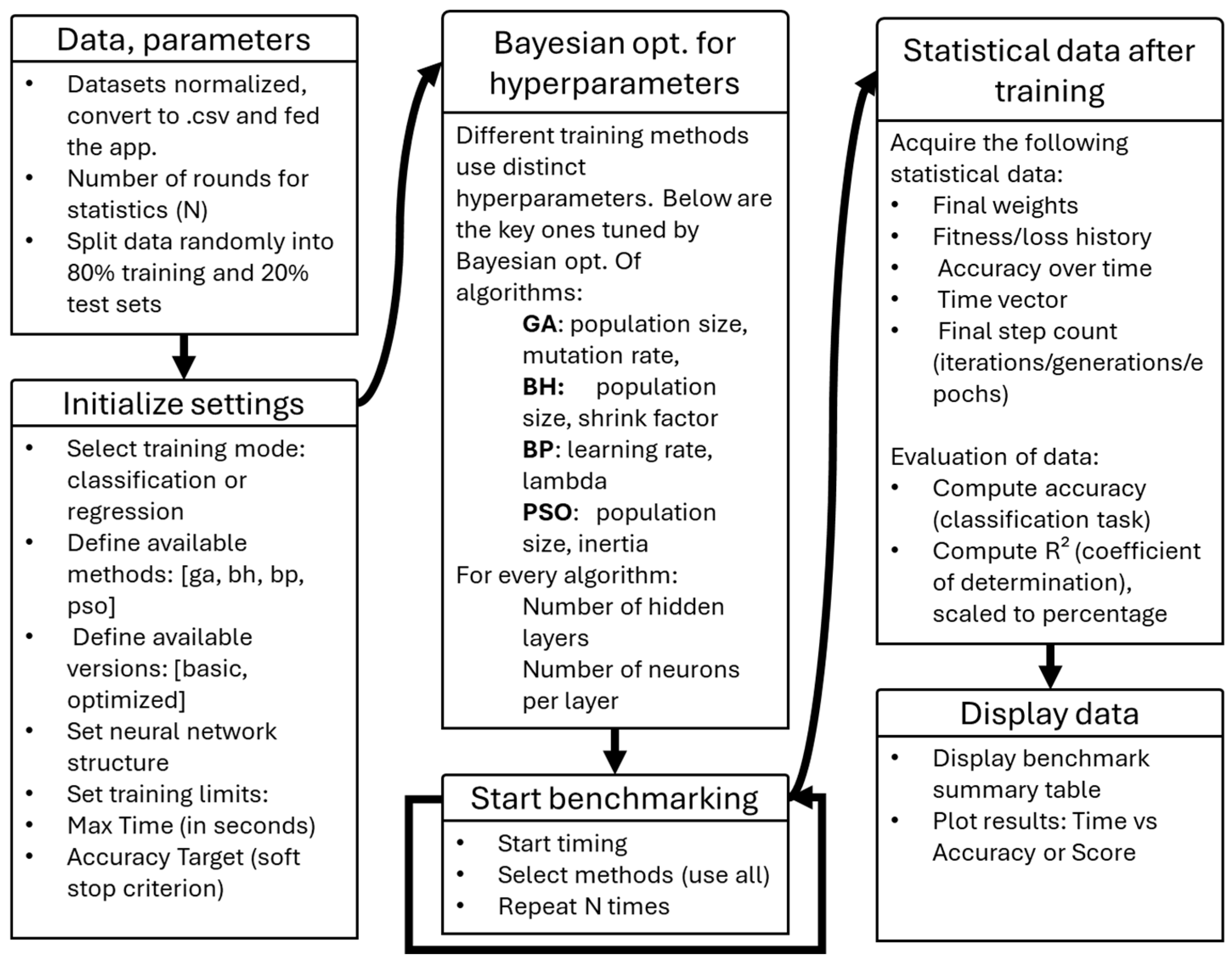
The testing process which we can see in
Figure 1 outlines a basic system for evaluating various neural network training algorithms using repeated statistical trials and Bayesian hyperparameter optimization. The dataset is first normalized and converted to a compatible format, then randomly split into 80% training and 20% testing sets. The system supports multiple training modes (here: classification or regression) and allows selection among the previously mentioned algorithms, each in either a basic or optimized variant. We can define key training constraints, including network architecture, maximum training time, and a soft accuracy target for early stopping. In our case, the training time was limited to a maximum 20 s or until the algorithm reached 99% accuracy, whichever occurred first.
Hyperparameters significantly influence the learning behavior and performance of neural networks. Unlike model weights, they are not learned during training but must be set externally. For each method, the optimization targeted a minimal yet impactful set of parameters—such as learning rate (BP), population size (GA, BH, PSO), mutation rate (GA), and inertia weight (PSO). Common architectural parameters, including the number of hidden layers and neurons, were also optimized. Bayesian optimization iteratively explored the parameter space using a surrogate model to maximize accuracy (for classification) or R2 (for regression), all under a fixed time constraint.
After we acquire the hyperparameters, the training can start. During each training cycle, the system collects critical performance data: loss and accuracy curves, final weights, step counts, and time vectors. For classification tasks, accuracy is computed, while for regression, the R2 score (coefficient of determination) is calculated and scaled to percentage. The process is repeated N times to ensure statistical significance.
Final outputs include a benchmark summary table with mean and standard deviation values and performance plots visualizing time versus accuracy or score. This design supports robust comparative evaluation of training methods and their hyperparameter configurations.
2.1. Task Types: Classification and Regression
In this study, both regression and classification problems were used to test the algorithms under different learning conditions. In general, regression tasks involve predicting a continuous output value based on the input features, while classification tasks require assigning inputs to discrete categories, which is often easier for the methods [
30]. These two types of problems represent fundamentally different challenges for training algorithms and help to reveal their strengths and weaknesses in both precise estimation and categorical decision-making.
To acquire the training data, a small dataset was generated with randomly initialized input parameters in the range of [0, 1]. Each dataset contained 3000 individual training data points, differing in the number of input features; one such set included 4 input parameters.
For the regression task, a simple mathematical function was defined to calculate a representative value from the input features. This value, which falls within the range [0, 1], served as the target output for the regression models. The exact equation used is as follows:
where
is the
-th parameter
with the range of [0, 1]. Also,
are the representative numbers, and the categorization is the following:
This dual use of the same underlying value for both regression and classification ensures consistency in the testing framework while allowing a comprehensive evaluation of the algorithms in different learning contexts.
Table 1 presents the first 10 and last items as sample data points, including their input parameters, the calculated representative value, and the assigned categories for both the 3-class and 10-class classification schemes.
Instead of using a synthetically generated dataset, the second benchmark scenario was based on a real-world dataset, the Forest CoverType dataset, which contains 54 input parameters and is publicly available through the Scikit-Learn library or the UC Irvine Machine Learning Repository database. To ensure computational feasibility and consistency with our experimental framework, we extracted the first 10,000 samples and selected the first 10 integer-based features, which were subsequently normalized. This dataset provides a realistic classification challenge, as it contains both informative and non-informative features, along with natural noise inherent to environmental measurements. The target consists of seven forest-cover types (classes), making it an ideal testbed for multiclass classification tasks. For regression experiments, the second column (aspect) was extracted in its normalized form and used as the target value.
2.2. Algorithm Variant: Genetic Algorithm
The basic Genetic Algorithm is a population-based evolutionary method that searches for optimal weight combinations through mutation and crossover operations. In the implementation, key parameters such as population size, mutation rate and distribution, and the set of initial weights were made configurable. An additional feature the “Accuracy-drop rollback” was also added to the original GA version and later to the other methods, though it is rarely used in those. This mechanism retains the best-known solution if a generation results in a sudden drop in accuracy. It was introduced because, during early testing, the algorithm frequently lost high-performing individuals, leading to significant declines in accuracy without subsequent recovery. In many cases, this resulted in the algorithm becoming stuck in low-accuracy local minima. The rollback mechanism helps mitigate this issue by preserving stability and preventing the degradation of promising solutions across generations.
For optimization purposes, the following additions were implemented in the GA-optimized version, according to other researchers [
31]:
Fitness scaling: Fitness values were scaled using the formula , which improves selection sensitivity even for small differences in loss.
Elitism: The best-performing individuals (top 5%) are automatically carried over to the next generation, preserving high-quality solutions.
Alternating crossover: The algorithm alternates between linear and uniform crossover methods to maintain population diversity.
Gaussian mutation: Mutation is applied using Gaussian noise, balancing global exploration and local refinement.
Random individual injection: With a low (usually 10%) chance, entirely new individuals are introduced into the population to support exploration.
2.3. Algorithm Variant: Black-Hole Algorithm
The Black-hole Algorithm is based on a gravitational analogy, where candidate solutions (stars) are pulled toward the center of the population—the best solution, or the “black hole.” It employs simple yet effective update rules, which make it computationally efficient. This speed was a key reason for selecting it as a subject of investigation. The original version of the algorithm already functioned well without requiring structural changes. However, several improved variants have been proposed in the literature and through personal experimentation, which are believed to enhance its performance further. To develop an improved version, the following basic optimization techniques were incorporated, also by other researchers [
28]:
Fitness scaling: Enhances the robustness of the selection process, particularly in scenarios with slow convergence.
Adaptive star regeneration: Monitors the event horizon to dynamically reinitialize stars, helping the algorithm escape from local optima.
Accuracy-drop protection: Includes rollback and timeline correction mechanisms to prevent performance degradation after sudden drops in accuracy.
Compared to the Genetic Algorithm, sudden drops in accuracy were much less common with the Black-hole Algorithm. In some runs, they did not appear at all. Because of this, the accuracy drop protection feature was rarely needed.
2.4. Algorithm Variant: Backpropagation
The Backpropagation (BP) algorithm was used as a baseline due to its well-known speed and efficiency in training neural networks. As expected, it proved to be significantly faster than the metaheuristic methods—a trend that will become evident in the Results Section. Since Backpropagation is already highly optimized by design, it required little additional enhancement. However, a few common and easily implementable techniques were applied to improve generalization and stability [
12,
15,
32]:
Adam optimizer with parameters β1 = 0.9, β2 = 0.999;
Momentum, which is implicitly handled by the Adam algorithm;
L2 weight regularization with λ = 0.001;
Forward pass using sigmoid activations in hidden layers and softmax at the output;
Accuracy-drop protection to preserve the best model in case of sudden performance decline.
2.5. Algorithm Variant: Particle Swarm Optimization
Particle Swarm Optimization is inspired by the collective behavior of bird flocks or fish schools. Each candidate solution—referred to as a particle—moves through the search space by combining its own experience with that of its neighbors [
18]. The algorithm relies on simple update rules for position and velocity, making it both conceptually straightforward and computationally efficient. Due to its ability to balance exploration and exploitation through a limited set of well-defined parameters, PSO was selected as one of the evolutionary algorithms for benchmarking. The basic version of PSO was implemented using its original formulation, which includes only inertia-weighted velocity updates and static values for the learning factors. This baseline version demonstrated acceptable performance, particularly in regression tasks, but often converged prematurely or stagnated in more complex classification settings.
To improve its stability and convergence behavior, an optimized variant was also developed. The enhancements introduced in this version were based on widely accepted best practices in the PSO literature and experimental tuning. These include the following:
Inertia weight scheduling: dynamically adjusts the influence of previous velocity to encourage exploration early on and fine-tuning later in training.
Adaptive cognitive and social coefficients: allow particles to shift emphasis between personal bests and global bests based on training progress.
Velocity clamping: prevents particles from overshooting promising regions by limiting velocity magnitudes.
Random reinitialization of stagnant particles: helps avoid stagnation by replacing particles that fail to improve over several iterations.
Unlike the Black-hole Algorithm, which often converged smoothly, PSO exhibited more oscillatory behavior, particularly in classification tasks. However, the optimized version effectively reduced erratic movement, leading to more stable convergence and improved final accuracy in most scenarios
The previously mentioned algorithms, along with the performance-improving modifications, are also illustrated with pseudocode on
Figure 2.
3. Execution and Evaluation Setup
Before the training process is initiated, Bayesian hyperparameter tuning is first executed for each algorithm. Under the current configuration, the optimizer is allowed to explore the parameter space for up to 20 iterations, with each evaluation capped at 20 s, following the selected strategy. In the case of
Table 2, this was a classification task using the GA-OPT method on a four-parameter dataset with three target categories. As shown in the table, the winning configuration emerged in iteration 10, as also indicated in italics. For this relatively small-scale problem, the optimal network structure was determined to be two hidden layers with a [
1,
6] neuron arrangement, a mutation rate of 0.29332, and a population size of 21. The final training process for the algorithm is subsequently carried out using these tuned hyperparameters.
To ensure consistency and fairness across methods, Bayesian hyperparameter tuning was also performed for the remaining training algorithms under the same experimental conditions. The resulting hyperparameter settings for all four optimized variants are summarized below, where P1 and P2 refer to the method-specific parameters:
GA: P1 = population size, P2 = mutation rate
BH: P1 = population size, P2 = shrink factor
PSO: P1 = population size, P2 = inertia (velocity damping factor)
BP: P1 = learning rate, P2 = lambda (L2 regularization strength)
It should be noted, however, that if a basic version of the algorithm does not support one of the tuned parameters, such as the shrink factor in the basic implementation of the Black-hole Algorithm, that parameter is calculated but simply ignored, and the default behavior is retained.
Table 3 presents the final configurations obtained through Bayesian optimization for all eight algorithm variants; each applied to the same task type as in
Table 2. These settings are displayed for illustrative purposes only, and although they were used in the benchmark runs, they were not explicitly queried or reported at every stage of the evaluation.
After the lengthy hyperparameter setting, the training-phase can initiate. In most cases, the runtime of each experiment was limited to 20 s for 4-parameter tasks and 120 s for the 54-parameter tasks, which proved sufficient for the majority of tasks. In certain cases, especially for the optimized versions of the algorithms on the real-life dataset, the time limit was insufficient to obtain meaningful results; it only allowed for observing the convergence speed and behavior. These more complex configurations naturally required more computation time due to their larger search space and additional processing steps.
3.1. Testing of Classification Problem of Algorithms
The first scenario of the classification testing represents the simplest case: the algorithms were tasked with classifying 3000 samples into three classes based on an input dataset containing four parameters. The hyperparameters used were those introduced earlier, along with fixed configuration settings that remained unchanged throughout the experiments. Even after just 20 s of runtime, the results are already clearly visible.
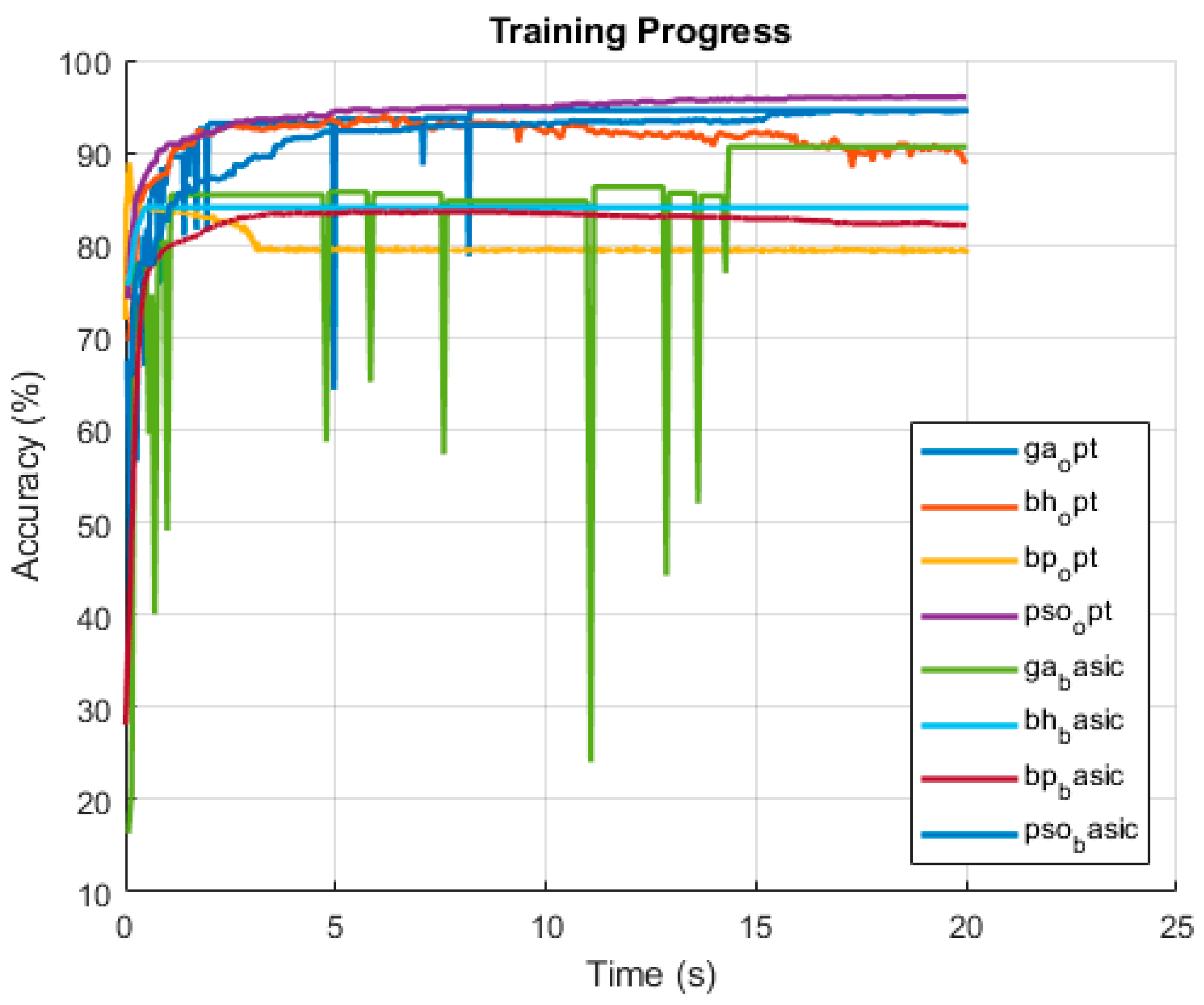
Figure 3 shows the final accuracy values from the last iterations of 20 independent runs, each capped at 20 s. This visualization setup will remain consistent across all subsequent figures, with only the time limit varying in scenarios involving larger datasets.
Table 4, as well as all the evaluation tables for the other runs, should be interpreted as follows: The method name is followed by columns showing the average accuracy and standard deviation at 1, 4, and 10 s in the run, respectively. These early-stage metrics help illustrate how the algorithms behave at the beginning of the optimization process and highlight which ones appear most promising. The fifth column presents the final accuracy result using the same statistical format. This is followed by the average runtime and its standard deviation, and then the F1 score with the same metrics, which is a key indicator in classification tasks. Although typically associated with classification, the F1 score can also be computed in regression settings, and this application does so automatically. Finally, the number of steps in the last run is listed. We can refer to them as ‘steps’ to cover the terminology used by different algorithms—such as ‘epochs’ for backpropagation and ‘iterations’ or ‘generations’ for others. In the following tables, the best results in terms of average scores and F1 values are highlighted in bold for better readability.
As shown in
Figure 3 and
Table 4, all algorithms reached or exceeded 80% accuracy within 20 s. GA-opt improved steadily, outperforming its basic version, though with higher variability. BH-basic and BH-opt both showed strong early performance, with BH-opt slightly ahead. PSO methods performed exceptionally well, with PSO-opt achieving the highest accuracy (94.03%) and PSO-basic closely behind. BP-basic also delivered excellent stable results, slightly outperforming its optimized version. Overall, PSO and BP variants led in performance, demonstrating that even under short time constraints, high accuracy is achievable on simpler classification tasks.
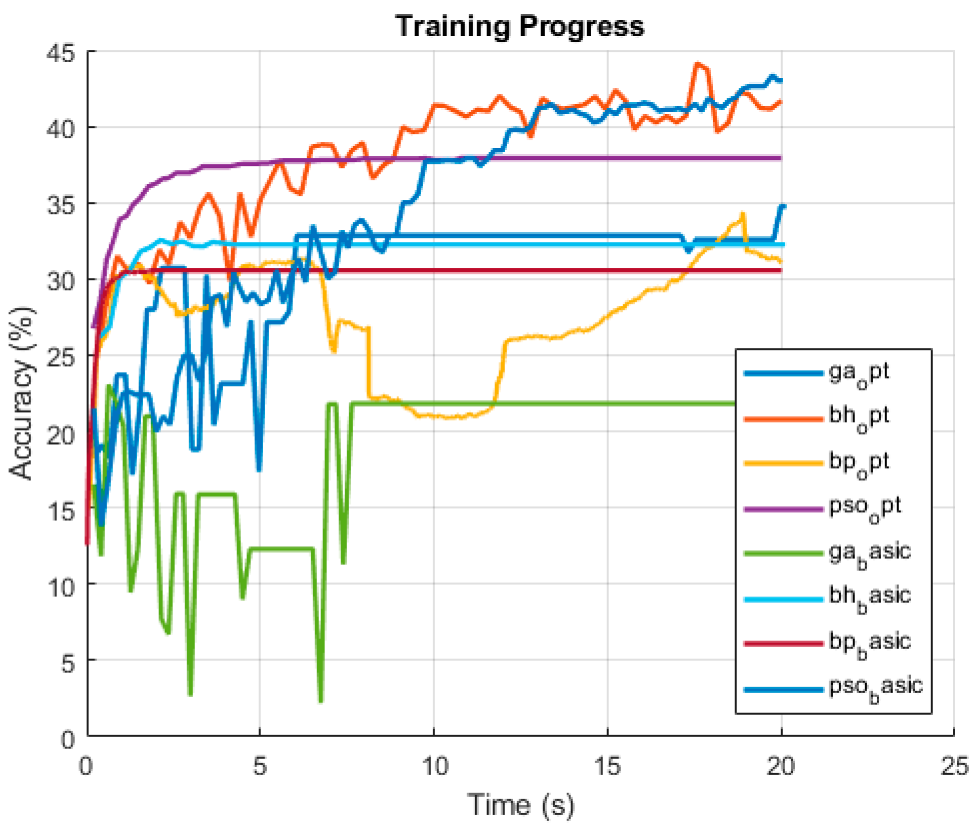
The second task was conducted on the same dataset, using four input parameters but with ten classification outputs. In this case, the 20 s runtime proved insufficient to achieve acceptable accuracy levels. Nonetheless, useful observations can still be made.
Figure 4 illustrates the result of a single representative run, while
Table 5 summarizes the evaluated outcomes from 20 independent runs. These results provide insight into the convergence behavior and offer a basis for predicting longer-term performance. While we do not have precise data on this aspect, it was apparent that most algorithms trained using a significantly larger architecture: typically, with two hidden layers and between 50 and 100 neurons, likely due to the increased complexity of having ten output classes.
The PSO optimized version showed the strongest overall performance, clearly outperforming the others both in early and final accuracy, consistently rising throughout the training. BH-opt also performed well, starting strong and improving steadily throughout the run, surpassing both PSO-basic and BH-basic in final accuracy. BH-basic, while initially promising, quickly plateaued and showed little improvement after the first few seconds. BP-based methods struggled to achieve competitive results under the time constraint, although their optimized version exhibited slight improvements. GA-basic, similar to the first experiment, demonstrated relatively low and stagnant performance throughout. The accuracy curves reflect these trends: PSO-opt consistently climbs and stabilizes at the top; BH-opt and GA-opt show fluctuating but improving trends; while BP and GA basic versions plateau early. These dynamics confirm that, under short training times and with increased output complexity, convergence speed and early adaptation significantly influence performance rankings.
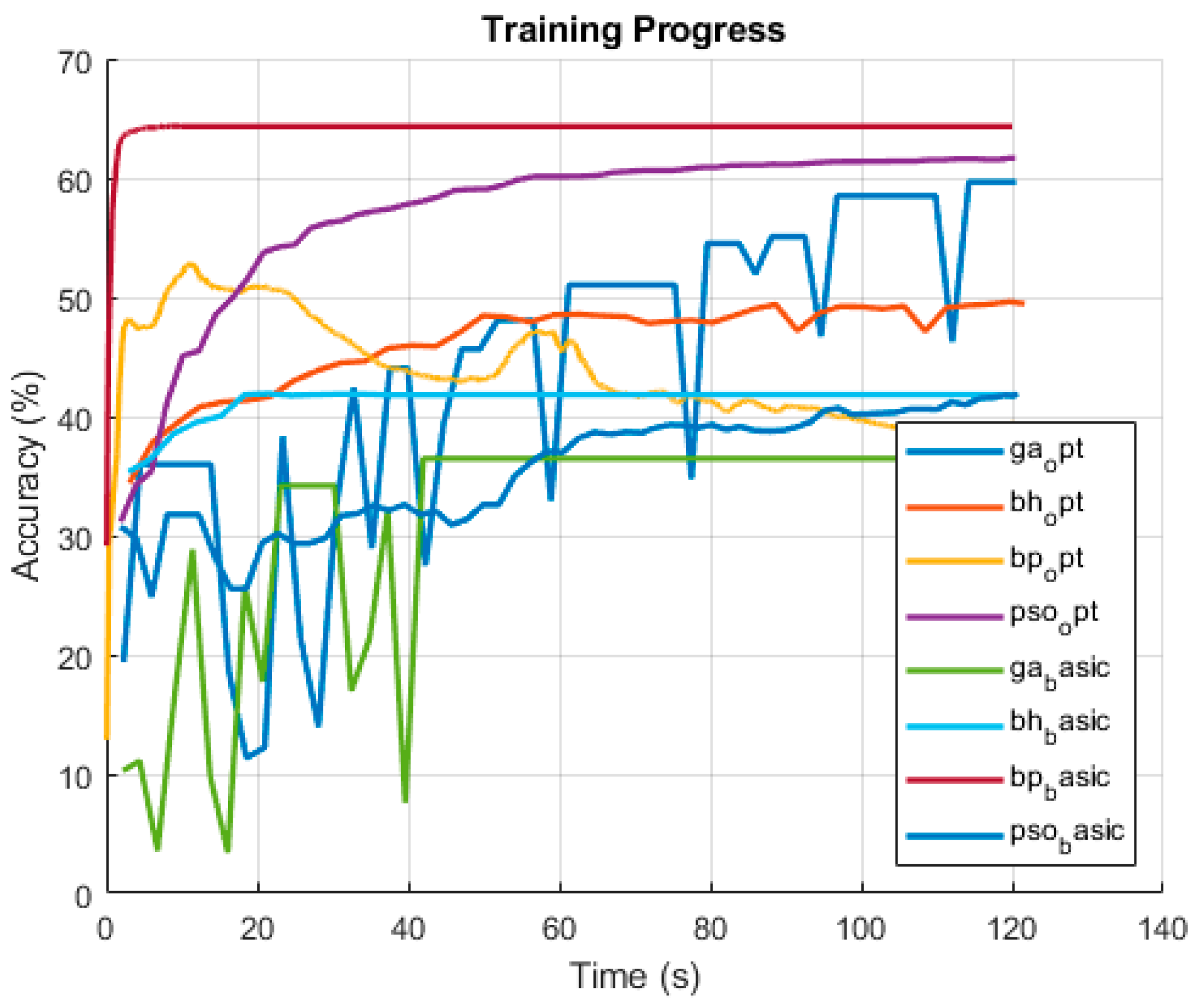
The final classification task was carried out using the real-world Forest CoverType dataset, which contains 54 input features and seven output classes. In this case, the 20 s runtime was far from sufficient, even to observe convergence trends. Therefore, each run’s time was extended to 120 s to better assess the algorithms’ behavior under more realistic conditions.
In the test runs, which can be seen in
Figure 5 and
Table 6, GA-opt demonstrated the strongest improvement over time, achieving the highest final accuracy (58.56%) and showing a consistent upward trend throughout the training. PSO-opt followed closely, with a similarly smooth and high-performing learning curve, reaching 57.94% final accuracy and a strong F1 score (0.38). BH-opt also performed very well in this setup, steadily improving from the beginning and stabilizing at a competitive 53.34%, surpassing its basic counterpart. PSO-basic showed robust and stable learning, finishing at 53.72%, essentially matching BH-opt in final accuracy and F1.
BP-basic started at a remarkably high level and remained stable throughout, finishing at 54.80% accuracy and delivering the best F1 score (0.40). Its optimized version (BP-opt) exhibited greater variance but achieved nearly the same final accuracy (54.72%), showing strong potential when allowed extended time. BH-basic, although stable and relatively strong early on, plateaued earlier than its optimized version, reaching 41.32%. GA-basic improved slowly but steadily, ending at 33.54%, much lower than the optimized GA.
To summarize the classification tasks, PSO-opt consistently delivered the best performance across tasks, showing steady improvement and reaching the highest final accuracy in both short and extended training. GA-opt also improved reliably over time, clearly outperforming GA-basic, which remained low and variable. BH-opt showed strong early progress and outperformed BH-basic, which plateaued quickly after an initially promising start. BP-basic maintained stable, high performance with the top F1 score, while BP-opt showed more variance but nearly matched its final accuracy when given more time. Overall, PSO and BP variants proved to be the most robust, especially under time constraints and increasing task complexity
3.2. Testing of Regression Problem of Algorithms
Regression analysis differs somewhat from classification, particularly in how performance is measured. It is generally more difficult to evaluate, as traditional accuracy metrics do not directly apply in the same way. To maintain a consistent scale and allow for intuitive comparison across models, the following custom regression accuracy formula—used by others but slightly modified to better suit this study—was employed as follows [
13,
15]:
where
is the prediction of the target;
is the actual target value;
is the number of data; and
is the maximum value of the full target value range. In this equation, the first component of the custom accuracy metric corresponds to the Mean Absolute Error (MAE), while the second part acts as a scaling factor that transforms the values into a 0–100% range based on the maximum observed target value. The resulting percentage expresses how close the predicted value is to the actual target, making the output easier to interpret visually. However, it is important to emphasize that this percentage-based accuracy is used solely for visualization purposes. All actual learning, optimization, and evaluation processes are still based on the Mean Squared Error, which remains the core loss function throughout the whole experiments.
The first of the two tasks involves predicting values generated from a regression formula based on the 4-parameter dataset. This should not pose a significant challenge for the algorithms, even though regression is generally considered a considerably more difficult task than classification.
As shown in
Figure 6 and
Table 7, PSO-opt achieved the best overall performance in this experiment, maintaining a steady upward trend and reaching the highest final accuracy (48.18%). BH-opt also performed well, showing consistent improvement and finishing slightly below PSO-opt. GA-opt improved gradually but remained behind the top performers, while its basic version (GA-basic) stayed at a significantly lower level with limited progression. BP-basic and BP-opt produced similar final results (~35%), but their learning dynamics differed—BP-basic was stable, whereas BP-opt showed more fluctuation and slower early convergence. PSO-basic also showed strong growth, ending just below 40%, outperforming several optimized methods. In general, PSO and BH algorithms dominated this setting, with PSO-opt standing out for both accuracy and stability. The figure clearly reflects these trends, highlighting how convergence speed and early adaptability shape algorithmic success under time-limited conditions.
As previously mentioned, the regression task on the real dataset was designed by removing one normalized integer feature (specifically, the second column) from the Forest CoverType dataset. The models were then tasked with predicting this target variable using the remaining 53 input features. This modification turned the original classification setup into a regression problem while preserving the dataset’s real-world complexity. The following results were obtained during the experiments.
As shown in
Figure 7 and
Table 8, BP-basic delivered the most stable and highest performance throughout the regression task, maintaining around 65% accuracy with minimal variance and achieving the best F1 score (0.53). BP-opt also performed well, with continuous improvement and a strong final accuracy (56.06%), though with slightly more fluctuation. PSO-opt showed the steepest learning curve among the evolutionary methods, reaching 59.74% accuracy by the end, while PSO-basic was more unstable but still competitive. GA-opt improved steadily, ending with a strong 54.76%, a significant gain over its basic version, which showed poor and erratic behavior. BH-based methods performed moderately, with BH-opt outperforming its basic version, although both plateaued below 45% accuracy. Overall, BP variants led the regression task, followed by PSO-opt and GA-opt, highlighting the advantage of gradient-based methods and well-optimized heuristics in handling continuous output prediction.
Across the regression tasks, BP-basic consistently delivered the most stable and accurate performance, particularly in the more complex setting, with the highest F1 score. BP-opt also performed well, though it showed greater fluctuation and slightly lower final accuracy. PSO-opt emerged as the strongest evolutionary method in both experiments, showing steep, steady improvement and achieving the highest or near-highest accuracy overall. GA-opt showed steady gains but remained behind PSO and BP, while BH-opt improved moderately and plateaued below the top performers. Overall, gradient-based methods (especially BP) led the regression tasks, but PSO-opt demonstrated the best balance between convergence speed, stability, and final accuracy among heuristic approaches.
4. Discussion
This study compared three training algorithms, the commonly used Genetic Algorithm, Particle Swarm Optimization, and Backpropagation, with the novel Black-hole Algorithm across multiple neural network learning tasks, including classification and regression, using both low-dimensional (4 input parameters) and medium-dimensional (54 input parameters) data.
Clear performance patterns emerged throughout the experiments. Backpropagation consistently delivered the most stable and accurate results in regression tasks, particularly in more complex scenarios, achieving the highest F1 score. PSO-opt showed the most robust and consistent learning among the heuristic methods, performing best in classification and remaining highly competitive in regression. GA-opt improved steadily but generally lagged behind PSO and BP, while its basic version showed limited effectiveness.
The Black-hole Algorithm demonstrated strong early convergence across tasks, frequently outperforming other methods in the first seconds of training. However, its final accuracy plateaued in both classification and regression tasks, falling short of the top-performing methods. Still, its early-stage efficiency and moderate stability, especially compared to GA-basic, highlight its potential value in hybrid approaches or early-stage optimization. BH-opt regularly outperformed BH-basic, confirming the benefits of proper parameter tuning.
One of the key insights from this study is that no single algorithm performs best across all settings. Gradient-based methods like Backpropagation dominate in regression, while optimized PSO variants excel in classification. The Black-hole Algorithm offers a compelling advantage in early convergence speed and could be particularly useful in multi-phase training pipelines, where rapid initial exploration is valuable before switching to fine-tuning algorithms such as BP or the GA.
To strengthen the evaluation, the proposed method was compared to several commonly used baseline techniques. However, the importance of benchmarking against more recent and advanced approaches is acknowledged. Although a detailed comparison with the latest metaheuristic or data-driven models was beyond the scope of this study, we recognize this as a valuable direction. Therefore, a follow-up study is currently being prepared to include such comparisons and extend the experimental framework accordingly.
Based on the findings of this study, several directions for future research appear promising. One such direction is the exploration of hybrid training strategies, where different algorithms contribute in complementary ways. For example, the Black-hole Algorithm’s fast initial convergence could serve to provide good starting weights, followed by PSO or Backpropagation for fine-tuning. Finally, leveraging hardware acceleration like GPUs could improve the practicality of population-based methods for larger-scale problems.
5. Conclusions
This study systematically compared four neural network training algorithms, the Genetic Algorithm, the Black-hole Algorithm, Particle Swarm Optimization and Backpropagation, across both classification and regression tasks using controlled, custom-designed, and real-world datasets. All methods were implemented from scratch in MATLAB without relying on pre-optimized toolboxes, ensuring that performance differences arose solely from inherent algorithmic behavior.
The test scenarios involved a synthetic dataset and the Forest CoverType dataset, with either 4 or 54 input parameters. From these, both regression tasks (predicting a continuous representative value) and classification tasks (categorizing the value into 3, 7, or 10 classes) were derived. A consistent network architecture was used, scaled according to input size, and each algorithm was tested in both basic and optimized versions. The study also incorporated practical constraints such as a 20/120 s runtime cap and Bayesian hyperparameter optimization in the beginning of each test.
Clear patterns emerged in the experiments: Backpropagation excelled in regression, while the optimized PSO algorithm led in classification and remained competitive elsewhere. The optimized GA showed steady but modest gains, and the basic version underperformed overall. The Black-hole Algorithm consistently demonstrated strong early convergence, often outperforming others in the initial seconds, though it generally plateaued below the top performers in the long run. Still, it showed improved results with tuning and greater early-phase stability than the GA. While the BHA was not the overall strongest, it was never far behind, making it a promising candidate for hybrid strategies and worthy of further investigation.


