Abstract
To improve the accuracy of heating load forecasting and effectively address the energy waste caused by supply–demand imbalances and uneven thermal distribution, this study innovatively proposes a hybrid prediction model incorporating seasonal adjustment strategies. The model establishes a dynamically adaptive forecasting framework through synergistic integration of the Sparrow Search Algorithm (SSA), Variational Mode Decomposition (VMD), and Long Short-Term Memory (LSTM) network. Specifically, VMD is first employed to decompose the historical heating load data from Arizona State University’s Tempe campus into multiple stationary modal components, aiming to reduce data complexity and suppress noise interference. Subsequently, the SSA is utilized to optimize the hyperparameters of the LSTM network, with targeted adjustments made according to the seasonal characteristics of the heating load, enabling the identification of optimal configurations for each season. Comprehensive experimental evaluations demonstrate that the proposed model achieves the lowest values across three key performance metrics—Mean Absolute Percentage Error (MAPE), Mean Absolute Error (MAE), and Root Mean Square Error (RMSE)—under various seasonal conditions. Notably, the MAPE values are reduced to 1.3824%, 0.9549%, 6.4018%, and 1.3272%, with average error reductions of 9.4873%, 3.8451%, 6.6545%, and 6.5712% compared to alternative models. These results strongly confirm the superior predictive accuracy and fitting capability of the proposed model, highlighting its potential to support energy allocation optimization in district heating systems.
Keywords:
heating load forecasting; seasonal adjustment; variational mode decomposition; long short-term memory network; sparrow search algorithm MSC:
68T01
1. Introduction
Amid the ongoing surge in global energy demand and the growing prominence of environmental concerns, enhancing energy efficiency and optimizing the energy mix have emerged as pressing global challenges. In response to the national directive outlined in the “Energy Production and Consumption Revolution Strategy (2016–2030)”, urban heating systems are accelerating their transition toward low-carbon development by actively promoting heating strategies centered on green and low-carbon energy sources, gradually phasing out traditional coal-based methods. By leveraging the advanced concept of intelligent heating and integrating artificial intelligence technologies with optimization algorithms, it becomes possible to significantly improve the operational efficiency of heat exchange stations, precisely avoid excessive heating, and substantially reduce energy waste—thereby facilitating the steady evolution of heating systems toward greener and more sustainable solutions. As a pivotal component of energy management and dispatch, heating load forecasting plays a crucial role; its accuracy directly impacts the balance between supply and demand, system efficiency, and economic performance. Accurate forecasting is thus essential for ensuring the stability, economic viability, and environmental sustainability of heating operations. Developing a high-precision, highly reliable heating load prediction model [1] holds not only significant theoretical value but also profound practical implications. Furthermore, within the framework of integrated energy systems [2], renewable energy sources such as geothermal, biomass, and solar energy are increasingly being incorporated into heating networks. This integration not only helps to alleviate the challenges of energy scarcity but also contributes to a substantial reduction in greenhouse gas emissions, offering a proactive means of mitigating environmental pressures.
Traditional approaches to heating load forecasting primarily rely on statistical models, machine learning algorithms, and deep learning techniques. Statistical models focus on analyzing historical data in depth and constructing corresponding mathematical frameworks to enable forecasting. Well-established methods such as Multiple Linear Regression (MLR) [3], Autoregressive Moving Average (ARMA) [4], and the Seasonal Autoregressive Integrated Moving Average (SARIMA) [5], which accounts for seasonality, have been practically applied in the domain of heating load prediction. In contrast, machine learning algorithms leverage large volumes of training data and a diverse range of techniques to develop predictive models. Methods including Support Vector Machine (SVM) [6], Random Forest (RF) [7], XGBoost [8], and Artificial Neural Network (ANN) [9] have also demonstrated strong performance in heating load forecasting tasks.
In recent years, artificial intelligence—particularly deep learning—has experienced groundbreaking advancements, emerging as a focal point within the AI domain. Deep learning emulates the functioning of the human brain by constructing multilayer neural networks, and through training on large-scale datasets, continuously enhances both prediction accuracy and generalization capability. Within the energy sector, deep learning has been extensively applied to areas such as load forecasting, energy consumption optimization, and equipment fault detection, demonstrating exceptional performance. It has now become a mainstream approach for short-term heating load prediction. Specifically, widely used deep learning architectures such as Recurrent Neural Networks (RNNs) [10], Temporal Convolutional Networks (TCNs) [11], and Long Short-Term Memory (LSTM) networks [12] have seen broad adoption in heating load forecasting. Other models like Gated Recurrent Units (GRUs) and Bidirectional LSTM (Bi-LSTM) [13] have also shown promising potential in this area. For instance, Wang et al. [14] employed nine machine learning methods alongside three heuristic algorithms for heating load prediction, and their results indicated that LSTM, as a specialized form of RNN, yielded the most accurate forecasts. However, as the forecasting horizon extends, the performance of LSTM tends to degrade significantly, and the model becomes increasingly sensitive to data nonstationary and noise. When applied directly to raw, nonstationary heating load data, LSTM is prone to overfitting and a noticeable drop in predictive accuracy. To address these challenges, recent research has shifted toward developing hybrid models that integrate deep learning with signal decomposition techniques and optimization algorithms to enhance the handling of nonstationary data. For example, Wang et al. [15] utilized correlation analysis grounded in statistical theory to examine the relationships between heating demand and influencing factors, selecting relevant input features accordingly. Their comparative study of models such as PSO-SVM, SVM, GA-SVM, and GA-ANN revealed that the PSO-SVM configuration delivered the best forecasting performance. Additionally, Transformer-based models [16] have been applied to short-term forecasting of integrated energy loads at the user level, offering more balanced accuracy and improved efficiency. Gao et al. [17] proposed a hybrid forecasting model combining a Generalized Regression Neural Network (GRNN) with LSTM, optimized using the Beetle Antennae Search (BAS) algorithm. Applied to building cooling load forecasting, this BAS-GRNN&LSTM model demonstrated notable advantages in terms of robustness and generalization ability.
Hybrid models, despite their advantages in load forecasting, face practical challenges: their complex multi-sub-model integration raises development difficulty and time costs; differing sub-model characteristics often cause issues like local optima or suboptimal performance, limiting prediction effectiveness; and the nonlinear, stochastic nature of load data requires large high-quality samples, which are often scarce in practice, reducing accuracy. To tackle these, researchers are exploring combining optimization algorithms with deep learning to boost model efficiency and performance. Recent studies have proposed using various optimization methods—such as Particle Swarm Optimization (PSO) [18], the Gray Wolf Optimizer (GWO) [19], and the Sparrow Search Algorithm (SSA) [20]—to fine-tune model parameters. However, most of these applications have been focused on feature parameter extraction in fault diagnosis, with relatively limited exploration in load forecasting scenarios. Notably, compared with PSO, which tends to suffer from premature convergence, and the GWO, which is prone to becoming trapped in local extrema, the SSA—by simulating the foraging and anti-predation behaviors of sparrows—offers a more effective approach to solving complex optimization problems. It features high search precision, fast convergence speed, and strong stability, while also effectively overcoming the issue of local optima, making it a promising tool for load forecasting applications. In the context of heating load forecasting, selecting an appropriate predictive model is crucial to improving accuracy and reliability. Traditional models such as Back Propagation (BP) neural networks and ARIMA have shown good performance in certain scenarios but are limited by their insufficient handling of temporal dependencies or inability to capture complex nonlinear relationships. In contrast, Recurrent Neural Networks (RNNs) and their advanced variant, the Long Short-Term Memory (LSTM) network, have become the preferred choices for complex time series forecasting due to their ability to model long-term dependencies and nonlinear dynamics. Specifically, LSTM, through its unique gating mechanisms, not only addresses the vanishing gradient problem of RNNs but also delivers outstanding performance in practical applications like heating load forecasting. For example, Yan et al. [21] proposed an improved BP neural network model that addressed challenges in nonlinear data prediction but still suffered from gradient vanishing and difficulty in configuring the hidden layers. Gavriel et al. [22] developed an innovative wavelet neural network that enhanced forecasting ability by using wavelet basis functions to locally amplify nonlinear features through a modified activation function. Meanwhile, Chen et al. [23] introduced an LSTM-based prediction model, which, as a representative of efficient Recurrent Neural Networks, effectively mitigated gradient vanishing and explosion issues encountered in traditional RNN training, thus making it more suitable for forecasting load data in energy systems.
In the field of heat load forecasting, the data often exhibit pronounced nonlinearity and nonstationary, compounded by the complex interplay of multiple external factors such as weather conditions and seasonal variations. These characteristics pose significant challenges for accurate modeling and prediction. Traditional single-model approaches struggle to fully capture the multi-scale features and long-term dependencies inherent in such data, thereby limiting improvements in prediction accuracy. To address these issues, signal decomposition techniques have been widely adopted in heat load forecasting, aiming to reduce data complexity and extract key features more effectively. Commonly employed methods include Empirical Mode Decomposition (EMD) [24], Ensemble Empirical Mode Decomposition (EEMD) [25], and Variational Mode Decomposition (VMD) [26]. EMD, known for its multi-resolution and adaptive capabilities, has shown unique advantages in signal processing; however, it suffers from mode mixing, which hampers the accurate extraction of information features. EEMD mitigates this issue by introducing noise-assisted signal processing techniques, effectively alleviating mode mixing. Nonetheless, the challenge of determining the optimal amplitude of the added white noise limits its practical applicability. In contrast, VMD, a more advanced signal decomposition technique, demonstrates significant advantages in heat load forecasting. It adaptively decomposes complex sequences into a series of modes with adjustable amplitude and frequency, effectively overcoming the difficulty of distinguishing frequency components encountered in EEMD. Moreover, VMD offers high computational efficiency, enabling rapid processing of large-scale datasets, which provides robust technical support for heat load prediction. Given these strengths, VMD holds considerable promise in this domain, offering a new avenue to enhance forecasting accuracy and reliability.
In recent years, the integration of Variational Mode Decomposition (VMD) and Long Short-Term Memory (LSTM) networks [27] has attracted substantial attention. VMD effectively decomposes raw heat load data into multiple relatively stationary sub-sequences, thereby filtering out noise and extracting multi-scale features to provide cleaner and more tractable inputs for subsequent modeling. LSTM excels at capturing long-term dependencies and nonlinearity in time series, suiting it to model temporal patterns in these sub-sequences. Combining VMD and LSTM boosts prediction accuracy and adaptability to complex heat load dynamics. Given substantial seasonal fluctuations in heat demand, season-specific models better capture trends for more accurate, reliable forecasting. In order to more accurately capture the seasonal change rule to improve the heat load prediction effect, the dataset from Arizona State University was selected because of its significant seasonal variation and complex dynamic characteristics. At the same time, because solving the traditional model optimization speed is slow and it is easy to fall into the local optimum of the difficult problem, this paper puts forward a combination of seasonal adjustment-based VMD-SSA-LSTM model prediction methods aiming at the unique characteristics of heat loads in different seasons. The novelty of the VMD-SSA-LSTM framework lies in its construction of a collaborative decomposition–optimization–prediction architecture: VMD adaptively decomposes heat load data into stationary IMF components to reduce modeling complexity; SSA optimizes LSTM hyperparameters to address the local optimum trap of traditional tuning methods; and LSTM accurately predicts and fuses these components, forming a closed-loop system of decomposition denoising, intelligent optimization, and temporal modeling. This three-stage integration deepens the coupling between signal decomposition and model optimization, enhances the capture of complex patterns, and outperforms single- or two-stage models in terms of robustness and prediction accuracy. The main contributions of this paper are as follows:
- A heat load prediction model based on VMD-SSA-LSTM is proposed, which effectively combines the advantages of the VMD algorithm in signal decomposition and the advantages of the LSTM model in time series prediction and provides a new way of thinking about nonstationary heat load prediction.
- The SSA is used to optimize the hyperparameters of the LSTM model, avoiding the blindness and computational complexity of the traditional grid search method, and improving the prediction accuracy and efficiency of the model.
- The public dataset of the integrated energy system of Arizona State University in the United States and the corresponding meteorological data are used for seasonal experimental verification. Under different seasons, compared with other models, the model in this paper achieves the best results in the three evaluation indexes of RMSE, MAE, and MAPE.
The overall structure of this paper is organized as follows: Section 1 focuses on the existing challenges in the field of heat load forecasting and proposes targeted solutions after systematically analyzing the root causes of the problems; Section 2 focuses on the basic theories of the SSA, LSTM, and VMD, covering the principles of the algorithms and analysis of the mathematical models; Section 3 describes the experimental design of the SSA, and introduces the complete process of VMD-SSA-LSTM hybrid model proposed in this paper from architectural design to specific implementation; Section 4 describes the sources of experimental data and preprocessing methods, clarifies the selection basis of evaluation indexes such as RMSE, MAE, MAPE, etc., and describes the experimental comparison strategy and parameter tuning process; Section 5 verifies the validity of the model through multi-dimensional comparison experiments to verify model validity, while conducting ablation experiments to quantify the contribution of each component (VMD, SSA) to the prediction accuracy; and Section 6 systematically summarizes the full text of the study.
2. Basic Theory
2.1. Long Short-Term Memory Network
Heat load data show significant temporal dependence, with current states closely linked to historical loads, making traditional static models ineffective in capturing temporal patterns. Researchers thus use Recurrent Neural Networks (RNNs), whose recurrent structure propagates historical information and works for short sequences. However, RNNs suffer from vanishing or exploding gradients in long sequences due to chain derivation, limiting performance—an issue well addressed by Long Short-Term Memory networks.
2.1.1. Principles of LSTM
Compared with vanilla RNNs, which use a single hidden state h, LSTM introduces a separate cell state C to serve as long-term memory. Unfolded along the time dimension, the network forms a chain-like structure in which, at each time step, it takes as input the current input , the previous hidden state , and the previous cell state , then outputs the new hidden state and updated cell state . The schematic structure is shown in Figure 1.
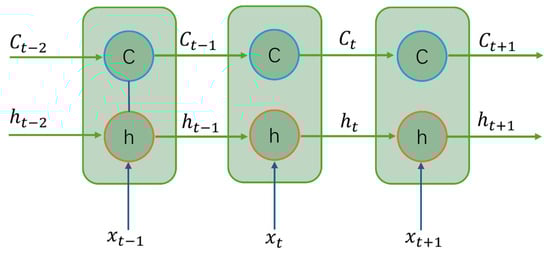
Figure 1.
LSTM schematic structure.
2.1.2. LSTM Structure
The network achieves dynamic information filtering through the synergistic operation of a triple gating mechanism consisting of a forget gate, an input gate, and an output gate. Its unit structure is illustrated in Figure 2.
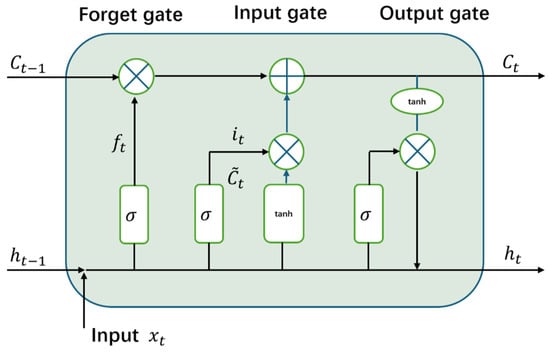
Figure 2.
Complete LSTM cell structure.
In the operating mechanism of LSTM, the forgetting gate receives the linear combination of the current input and the output at the previous moment and maps the combined values to the range of 0 to 1 through the Sigmoid activation function. When the output value approaches 1, the memory block will retain more historical information. When the output value approaches 0, the amount of information retained decreases accordingly. The calculation formula is as follows:
where denotes the output value of the forgetting gate; denotes the output value of the previous moment; denotes the current input value; denotes the bias matrix of the forgetting gate; and denote the weight coefficient matrix.
The input gate contains a two-layer structure: the Sigmoid layer is used to determine the information update ratio, and the tanh layer generates the new candidate vector to be fused. After linearly weighting the current input and the output at the previous moment in this Sigmoid layer, it is compressed to the interval [0,1] by the Sigmoid activation function . Its function is similar to that of the forgetting gate, but it focuses on quantifying the degree to which the current input information is integrated into the memory flow. The specific calculation formula is as follows:
where denotes the output value of the input gate; denotes the bias matrix of the Sigmoid layer of the input gate; and denote the corresponding weight coefficient matrix of the Sigmoid layer of the input gate.
The tanh layer of the input gate linearly combines the input value with the output of the previous moment, and generates the alternative value of the memory cell state through the tanh function, and then linearly combines with the state of the memory cell of the previous moment, to obtain the updated memory cell state . The corresponding formula is as follows:
where denotes the output value of the input gate; denotes the bias matrix of the tanh layer of the input gate; and are the corresponding weight coefficient matrices of the layer of the input gate.
The output gate controls the information that needs to be output in the memory cell through the Sigmoid activation function, and obtains the weight coefficient , then the output gate and the new cell state are generated through the tanh layer , to get the output value ; the corresponding calculation formula is as follows:
where denotes the weight matrix; denotes the bias matrix of the output gate; and denotes the output value of the output layer.
2.2. Sparrow Search Algorithm
In LSTM-based heat load prediction, hyperparameters—such as the number of hidden layers, learning rate, and number of training iterations—directly affect model architecture, convergence, and forecasting accuracy. However, tuning these in high-dimensional, nonconvex spaces is challenging. Traditional methods (manual tuning, grid search, and random search) are inefficient and resource-intensive, often becoming stuck in suboptimal local minima.
To address this, this study employs the Sparrow Search Algorithm (SSA), a meta-heuristic inspired by sparrow foraging and anti-predation behavior. The SSA combines strong global exploration with adaptive local search, making it well-suited for high-dimensional hyperparameter optimization. It categorizes the population into producers, followers, and sentinels: producers perform broad area exploration; followers conduct local exploitation; sentinels perform random walks to help escape potential local optima. This dynamic interplay enables efficient convergence to high-quality hyperparameter combinations.
2.2.1. Population Initialization
Initially the sparrow population, in which the position of each sparrow is randomly determined, is set. The population contains d × n sparrows, which is the candidate solution set of the optimization problem. Set the initial dimension d, where d is the number of targets that need to be optimized in the actual problem; n is the size of the population. The expression of the number matrix of sparrows is as follows:
During the algorithm initialization stage, the fitness value of each sparrow is assigned using a random initialization strategy. Subsequently, the fitness score of each sparrow is dynamically updated through an iterative process, driving the algorithm to continuously approach the better solution space. The mathematical expression of its initial fitness value is as follows:
Adaptation is calculated as
where represents the actual value of the i-th data point in the validation dataset and denotes the predicted value of the i-th data point output by the model.
2.2.2. Producer Location Update
During the algorithm operation stage, each sparrow initiates the update process from the initial state. The producer role prioritizes position adjustment, and its core task is to continuously explore the distribution of potential food resources. The mathematical expression for its position update is as follows:
where denotes the j-th dimensional parameter of the i-th sparrow in the t-th iteration; denotes the maximum number of iterations; is a uniform random number in (0,1]; ST is the safety threshold, which is taken to be a uniform random number in [0,1]; AL is the alarm value, which is taken to be [0.5,1]; Q is a standard normally distributed random number; and L is the unit matrix of 1 × d.
2.2.3. Follower Position Update
There are two core scenarios in the follower position update mechanism: First, when some followers obtain sufficient food resources through independent search, in order to maintain the dynamic balance of population roles, such individuals will take over the positions of some producers to complete the update. Secondly, when producers locate food sources, followers may seize their positions through a competitive mechanism, thereby triggering the location update process.
The equations for follower position update are as follows:
where denotes the best position occupied by the sparrow; denotes the worst position occupied by the sparrow; A is a 1 × d matrix with elements randomly taking 1 or −1. If , it indicates that the current position of the sparrow is unfavorable, as it has not successfully foraged for food. Therefore, it is necessary to expand the search range. If , the sparrow position is better, allowing for a more efficient localized search.
2.2.4. Vigilant Position Update
The number of vigilant individuals is set to be one fifth of the overall population, and their initial state positions are randomly generated.
Based on the rule of the iterative updating of producer and follower positions in a sparrow population, derive the corresponding positional update mathematical equation.
In the formula: represents the current central position of the population; is the regulatory parameter that follows the standard normal distribution; is a random value within the interval [−1,1]; is a minimal quantity approaching zero to avoid a zero denominator; represents the fitness value of the current sparrow individual; and correspond, respectively, to the optimal fitness and the worst fitness of the population. When > , this indicates that the sparrow is at the edge of the population and faces a higher risk of being preyed upon. When = , this indicates that the sparrow has sensed danger and has begun to move closer to other individuals to reduce the probability of being preyed upon.
The flow of the Sparrow Search Algorithm is shown schematically in Figure 3.
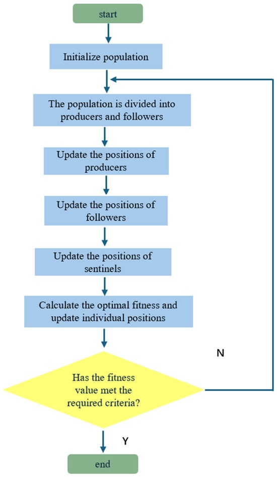
Figure 3.
Schematic flow of Sparrow Search Algorithm.
2.3. VMD Algorithm
Heat load data, as a nonlinear time series signal with multiple frequency components and complex dynamic characteristics, can be effectively decomposed using the Variational Mode Decomposition (VMD) algorithm. VMD achieves this by constructing a constrained variational model and iteratively solving the optimization problem via the Alternating Direction Method of Multipliers (ADMM), thereby decomposing the signal into Intrinsic Mode Functions (IMFs) with adaptively determined center frequencies and bandwidths. This approach avoids the mode aliasing issue inherent in traditional Empirical Mode Decomposition (EMD). Each IMF manifests as a frequency–amplitude modulation (FM-AM) signal with adjustable amplitude and frequency, and its mathematical expression is as follows:
where is the instantaneous amplitude function and the phase function is nondecreasing with ≥ 0. The analytical signal of the modal function is calculated through the Hilbert transformation to obtain the unilateral spectrum. Subsequently, the decomposed signal is mixed with its corresponding center frequency, and the spectra of each modal are converted to the fundamental frequency domain. The bandwidth of each mode is estimated based on the norm of the square of the gradient direction of the modulation signal, and its mathematical expression can be expressed as follows:
where is the k modal components obtained from the decomposition; is the center frequency of each component; is the convolution sign; and is the Dirac function.
The quadratic penalty factor and the Lagrange multiplier operator are introduced to transform the constrained variational problem into an unconstrained variational problem.
The alternating direction multiplier iterative algorithm is used to update and to solve the “saddle point” of the above equation, which is the optimal solution of the constrained variational model.
3. Model Design and Process
3.1. SSA Performance Test
To systematically evaluate the optimization performance of the Sparrow Search Algorithm (SSA), this paper conducts experimental simulation based on the CEC2005 test set [28]. This test set, as an internationally recognized standard for evaluating the performance of optimization algorithms, contains multiple sets of test functions with different characteristic attributes, and all are equipped with known optimal solutions or approximate optimal solutions. The comprehensive performance of the algorithm in terms of search efficiency, convergence speed, robustness and accuracy can be comprehensively examined. Through tests on the CEC2005 function set, the ability of the SSA to handle complex optimization problems can be objectively verified, providing a theoretical basis for its effectiveness in engineering scenarios such as heat load prediction. This paper selects four typical test functions F1 to F4 as the performance evaluation objects of the SSA, and their function expressions are detailed in Table 1.

Table 1.
F1 to F4 test functions.
Simultaneous comparison of PSO and GWO. Where the initial parameter settings are also set to a population size of 100 and 1000 iterations. The results of the algorithm testing are shown in Figure 4 below.
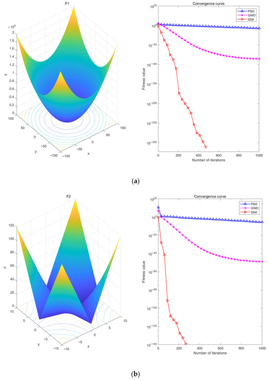
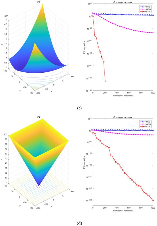
Figure 4.
Optimization Test Diagram of Function F1 (a), Optimization Test Diagram of Function F2 (b), Optimization Test Diagram of Function F3 (c), and Optimization Test Diagram of Function F4 (d).
Analyzing Figure 4, it can be seen that the SSA successfully finds the local optimal solution with a relatively small number of iterations, showing its fast convergence speed and high convergence accuracy. In particular, the best performance is on the F3 test function, which can approach the optimal solution with only about 200 iterations, while the GWO algorithm needs about 1000 iterations to approach the optimal solution gradually, and the worst news is that the PSO algorithm may need more than 1000 iterations to find the optimal solution. In addition, the SSA also has good performance in the other three test functions.
Comparative analysis demonstrates that the SSA (Sparrow Search Algorithm) outperforms both PSO (Particle Swarm Optimization) and the GWO (Gray Wolf Optimizer) in terms of optimization accuracy and convergence speed. This superiority makes the SSA particularly effective for LSTM hyperparameter tuning: (1) its excellent global search capability effectively avoids local optima, ensuring better parameter combinations; and (2) the fast convergence characteristic significantly reduces computational costs, especially on large-scale datasets. These advantages establish the SSA as an ideal optimizer for hyperparameter tuning of complex models like LSTM.
3.2. SSA Optimizes Hyperparameters of LSTM
Compared to traditional methods like manual hyperparameter tuning—which relies heavily on empirical knowledge, suffers from inefficiency, and often fails to find optimal solutions—the Sparrow Search Algorithm (SSA) offers distinct advantages in optimizing LSTM’s learning rate, number of hidden neurons, and training epochs. Given that LSTM, as a complex deep learning model, may exhibit intricate nonlinear interdependencies among its hyperparameters, the SSA is particularly well-suited to navigating such high-dimensional, nonlinear optimization landscapes. Furthermore, thermal load data typically exhibit nonlinear and nonstationary characteristics due to multiple influencing factors such as weather, season, and time. The SSA-optimized LSTM model demonstrates superior adaptability to these dynamic patterns, thereby enhancing both robustness and predictive accuracy. The specific steps for optimization are as follows:
- (1)
- Preprocess the data and construct the LSTM model.
- (2)
- Updating several population parameters such as population size, number of iterations, producer and follower ratios, and adjustment of learning parameter regions in a timely manner.
- (3)
- Calibrate the adaptation value of the Sparrow Search Algorithm, and dynamically adjust the search strategy and parameter settings according to the changes in the adaptation value. Based on the SSA, the RMSE is used as the objective function of optimization to find the best fitness.
- (4)
- The optimal fitness value is incorporated into the LSTM model for a certain proportion of training, resulting in an SSA-optimized LSTM prediction model.
- (5)
- Input the test heat load data and the prediction model outputs the predicted value of the test heat load. The specific process is shown in Figure 5.
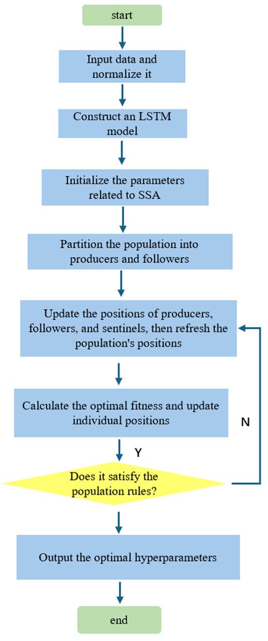 Figure 5. Schematic diagram of SSA-optimized LSTM.
3.3. VMD-SSA-LSTM Prediction Process
After introducing the VMD algorithm, the original thermal load data is first decomposed into a series of subcomponents. A VMD-SSA-LSTM model is then established for each decomposed sub-series, followed by further processing to predict the thermal load for individual sub-series. The predicted values of different sub-series are subsequently integrated to obtain the final thermal load prediction. Finally, the prediction results are validated, and the errors are analyzed. The detailed workflow is illustrated in Figure 6.
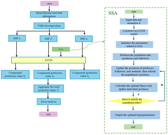
Figure 6.
Prediction flow of VMD-SSA-LSTM model.
4. Case Studies
4.1. Data Description
This paper adopts the public dataset of the integrated energy system released by Arizona State University in the United States [29]. This system integrates the data of power, cooling, and heating loads. The sampling frequency is set at once every hour, and the meteorological parameters of the corresponding period in this area are collected simultaneously [30]. It covers key meteorological characteristics such as wind speed, wind direction, precipitation, air pressure, DHI (Diffuse Horizontal Irradiance), DNI (Direct Normal Irradiance), GHI (Global Horizontal Irradiance), relative humidity, dew point, and temperature.
In this dataset, the heat load data has a clear seasonal variation. For example, heat loads are higher in winter, lower in summer, and in transition in spring and autumn. For this purpose the dataset was selected from March 2018–February 2019 and further subdivided in the original dataset into four seasonal datasets for spring, summer, autumn, and winter, and the ratio of the training set to the test set in each seasonal dataset was 7:3. The data and code for this experiment were written in MATLAB R2022a, and the hardware configuration was a 2.10 GHz with 16.00 GB of RAM AMD Ryzen 53550H CPU.
4.2. Data Pre-Processing
During the operation of an integrated energy system, due to factors such as sensor accuracy, transmission interference, and storage failures, outliers are likely to occur in heat load and associated environmental data (such as temperature and humidity) during the measurement, transmission, and storage processes. If these outliers are fed into the model, they will interfere with the training process: Invalid, null, or extreme outliers (such as data that clearly exceeds the normal load fluctuation range) will cause the model to fit unreasonable patterns; if outliers within the normal fluctuation range are directly discarded, potential key information will be lost, leading to an increase in model bias and a rise in the risk of overfitting.
Therefore, it is necessary to process the outliers before making predictions. For outliers that deviate significantly from the normal range, the following formula is used for processing.
where denotes the i-th abnormal value in the data.
The dimensional discrepancies between heat load data and environmental covariates (such as temperature and humidity) can impede the gradient update efficiency during model training, leading to slower convergence and diminished accuracy. To address this, In this paper, the data are normalized to the (0, 1) interval using the min–max normalization method, as defined by the following formula:
where represents the i-th normalized data point; denotes the total number of data points; is the i-th value in the original dataset; and and are the maximum and minimum values of the data, respectively. This normalization process eliminates the influence of dimensional units, enabling the model to learn data features more efficiently and enhancing both training speed and prediction accuracy.
In addition, to restore the normalized data to the dimensional scale of the original data, a denormalization operation is also required, and the formula is as follows:
where is the i-th data after normalization, and is the i-th value in the original data.
4.3. Evaluation Indicators
In this paper, Root Mean Square Error (RMSE), Mean Absolute Error (MAE), and Median Absolute Percentage Error (MAPE) are selected as quantitative evaluation indicators for the prediction accuracy of the model. These indicators can describe the deviation degree between the predicted values and the true values from multiple dimensions, providing a comprehensive and quantitative analysis basis for systematically evaluating the performance of the model.
where is the true value of the heat load; is the predicted value of the heat load; and is the number of the test sample set.
RMSE, MAE, and MAPE are commonly used quantitative criteria for assessing the accuracy of prediction models, where RMSE characterizes the arithmetic square root of the square of the deviation of the predicted value from the true observed value, MAE reflects the arithmetic mean of the absolute value of the prediction error, and MAPE expresses the mean of the percentage deviation of the predicted value relative to the true value. The smaller the values of the above indicators, the better the fitting effect of the prediction model, the higher the prediction accuracy and the smaller the relative error.
4.4. Parameter Setting
The parameters of the SSA are initialized, including the total population size, the number of hyperparameters for the optimization model, and the upper and lower bounds of the solution space. In this paper, the total population size is set to 3, and the number of hyperparameters for the optimization model is 3, these being the number of hidden layer neurons in the LSTM model (LayerNums), the maximum number of training epochs (MaxEpochs), and the optimal initial learning rate (Lr). The upper bound (Ub) and lower bound (Lb) for these three hyperparameters are set as shown in Table 2. The specific numerical values of the parameters after the SSA optimizes the model are presented in Table 3.
Table 2.
Upper and lower bounds for each parameter.
Table 3.
Optimized model parameters.
Analyzing the hyperparameter combinations for different seasons in Table 3, it was found through experiments that the required running times also vary. The heat load data differ across seasons. For the heat load in winter, the heat load changes relatively smoothly. When the SSA optimizes the LSTM hyperparameters, the population iteration converges relatively quickly, and under this experimental environment configuration, the running time is about 12 min. For the heat load in summer, as extreme high temperatures are more likely to occur and the data fluctuates strongly, the time consumed by the SSA for optimization will also increase, and the required time is about 40 min. Spring and autumn are transitional seasons, and abnormal weather conditions can easily occur, which will affect the change in heat load data and slow down the convergence speed of the algorithm. In spring and autumn, it takes about 24 min and 31 min, respectively.
4.5. Comparative Approach
In order to comprehensively evaluate the superiority of the VMD-SSA-LSTM model proposed in this paper, comparative experiments and ablation experiments were conducted. In the comparative experiments, three models, namely LSTM, CNN, and GRU, were selected to be compared with the model proposed in this paper, aiming to demonstrate the superiority of the proposed model. In addition, to assess the degree of influence of the SSA in optimizing the network structure of the VMD-LSTM in this paper, the method of ablation experiments was employed. Some components of the model were gradually removed and modified, and then evaluated. Through the above comparative experiments and ablation experiments, we can verify the superiority of the VMD-SSA-LSTM method over other models and determine the extent to which the SSA plays a role in optimizing the network structure to enhance the model’s performance.
5. Results and Discussion
In this study, we firstly use the traditional Long Short-Term Memory (LSTM) network model to predict the heat load data. To deeply analyze the correlation between heat load data and environmental impact factors, the Pearson correlation coefficient (PCC) method is introduced to quantify the linear correlation degree between each environmental factor and the heat load data. PCC, as a classic method for measuring the strength of linear association between two variables in statistics, has a value range of [−1, 1], where 1 corresponds to a completely positive correlation, −1 corresponds to a completely negative correlation, and 0 indicates no linear correlation. By calculating the influence weights of PCC-quantifiable environmental variables (such as temperature, humidity, wind speed, etc.) on the heat load, scientific support is provided for the screening of the input features of the model. The specific calculation formula of the PCC is as follows:
where PCC denotes the correlation coefficient of each influencing factor; denotes the i-th sample value of the heat load; denotes the i-th sample value of the environmental factor variable; and is the number of variables.
The Pearson correlation coefficient corresponds to the degree of correlation, as shown in Table 4, and its PCC correlation analysis thermal graph is shown in Figure 7.
Table 4.
Pearson’s correlation coefficient corresponding to the degree of association table.
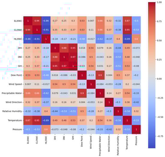
Figure 7.
Heat map for PCC correlation analysis.
According to the heat map analysis in Figure 7, temperature (Temperature), cooling load (CL(KW)), and electrical load (EL(KW)) are more relevant to the heat load data. Therefore, the above three characteristic factors were used as inputs to the LSTM model, which in turn was used to predict the heat load.
Secondly, we selected the VMD method to decompose the thermal load data. The decomposed components in the four seasons are shown in Figure 8. The five obtained components IMF1 to IMF5 were used as the input for the LSTM model, and then the prediction results of these five components were superimposed.
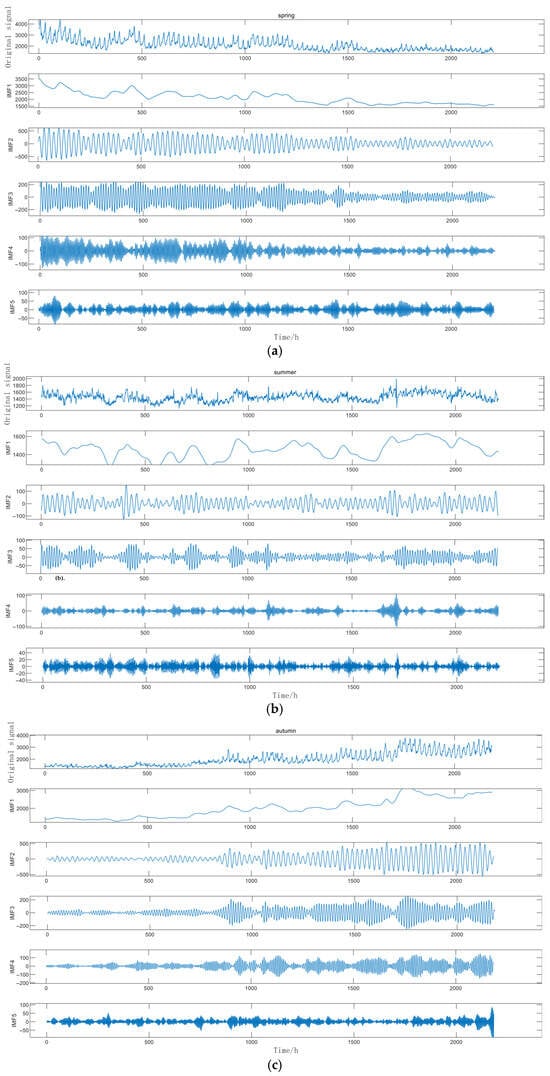
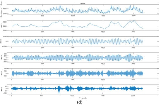
Figure 8.
Comparison Diagram of VMD Results in Spring (a), Comparison Diagram of VMD Results in Summer (b), Comparison Diagram of VMD Results in Autumn (c), and Comparison Diagram of VMD Results in Winter (d).
As depicted in Figure 8, it can be observed that for all the component data after decomposition, the vibration periods and fluctuation trends are alleviated when compared to the initial residual component. Generally speaking, the stationarity has been remarkably improved. The decomposed modes distinctly separate these trend and fluctuation components, which is conducive to the further analysis and prediction of the variations in thermal load.
Finally, the model proposed in this paper, which uses the SSA to optimize the VMD-LSTM model, is employed to search for the optimal parameter combination for thermal load forecasting. Comparative experiments are designed in this paper. The performance of the proposed VMD-SSA-LSTM model is compared with that of traditional models, and a comprehensive evaluation is carried out from multiple indicators such as RMSE, MAE, and MAPE. In addition, ablation experiments were also conducted. By removing modules such as SSA and VMD one by one, the contributions of each component to the model performance were analyzed to verify the rationality and necessity of the model structure. The experimental results demonstrate that the model proposed in this paper has remarkable superiority and robustness in the thermal load forecasting task.
5.1. Analysis of Comparative Experiments
5.1.1. Error Analysis of Comparative Models
In the field of thermal load forecasting, the accuracy of the forecasting model is of vital importance. In order to comprehensively evaluate the performance of different models in each season, we conducted a comparative analysis of the prediction errors of four different models—LSTM, GRU, CNN, and VMD-SSA-LSTM—on the data of the four seasons. The errors of the comparative models in different seasons are shown in Figure 9.
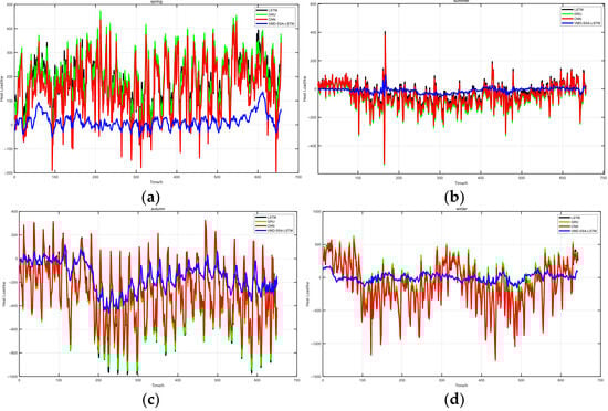
Figure 9.
Error Diagram of Comparative Models in Spring (a), Error Diagram of Comparative Models in Summer (b), Error Diagram of Comparative Models in Autumn (c), Error Diagram of Comparative Models in Winter (d).
In Figure 9a, the error diagram of comparative models in spring, the LSTM model shows obvious fluctuations, with many peaks and troughs, indicating that its prediction error varies greatly. The GRU model also has significant fluctuations, and the error amplitude is similar to that of the LSTM model. The CNN model has many error spikes with large amplitudes. In contrast, the VMD-SSA-LSTM model performs more stably, and the error values generally remain at a low level, which shows that this model has better performance when dealing with spring thermal load data. In Figure 9b, the error diagram of the comparative models in summer, the error fluctuations of the LSTM model are still irregular, and the error values of some peaks are relatively high. The error curve of the GRU model also changes greatly. The CNN model has multiple large error spikes. However, the VMD-SSA-LSTM model still maintains a relatively stable and low error level, demonstrating its robustness under summer conditions. In Figure 9c, which is actually the error diagram of comparative models in autumn, the LSTM model experiences a series of large-amplitude error fluctuations, indicating that it has difficulties in accurately predicting the thermal load in autumn. The error fluctuations of the GRU model are also quite obvious. The CNN model frequently has large errors. At the same time, the error variation in the VMD-SSA-LSTM model is relatively small and is easier to control, highlighting its effectiveness in capturing the complex patterns of autumn thermal load data. In Figure 9d, the error diagram of comparative models in winter, the error fluctuation range of the LSTM model is large, and there are some extreme error values. The error variation in the GRU model is also significant. The CNN model has multiple error spikes. On the other hand, compared with other models, the VMD-SSA-LSTM model maintains a relatively stable error trend, and the error values remain at a low level.
Overall, across the four seasons, compared with the LSTM, GRU, and CNN models, the VMD-SSA-LSTM model consistently demonstrates lower and more stable prediction errors. This indicates that, with its unique combination of technologies, the proposed VMD-SSA-LSTM model is more effective in handling the complexity of thermal load data in different seasons. It is a promising method for accurate thermal load forecasting.
5.1.2. Analysis of the Prediction Effects of Comparative Models
In order to better understand the prediction effects of different models and further demonstrate the superior prediction performance of the model proposed in this paper, in the analysis of the prediction results of the comparative models, we conducted seasonal prediction experiments for the four models, presenting the comparison of the prediction results of the four models on thermal load data in different seasons. The prediction results of the comparative models are shown in Figure 10.
Figure 10.
Prediction Results Diagram of Comparative Models for Spring (a), Prediction Results Diagram of Comparative Models for Summer (b), Prediction Results Diagram of Comparative Models for Autumn (c), Prediction Results Diagram of Comparative Models for Winter (d).
In Figure 10a, the prediction results diagram of comparative models for spring, the true value (the black curve) shows a fluctuating pattern. The LSTM follows the true value to some extent, but there are obvious deviations in many places, indicating that the LSTM model has limitations in capturing the details of spring thermal load. The trend for GRU is similar to that of the true value, but there are also some gaps. The CNN has a large deviation, which shows that the CNN model may not be very suitable for modeling the spring thermal load. In contrast, the curve of VMD-SSA-LSTM closely follows the true value, demonstrating its excellent ability to predict the spring thermal load. In Figure 10b, the prediction results diagram of comparative models for summer, the true value has its own fluctuation characteristics. The LSTM model has some deviations from the true value, especially in some peak areas. The GRU model also fails to closely fit the true value in some parts. The CNN model has obvious differences from the true value. However, the VMD-SSA-LSTM model is more consistent with the black curve, indicating that it has a good adaptability to the summer thermal load data. In Figure 10c, the prediction results diagram of comparative models for autumn, the true value also shows a complex fluctuating trend. The LSTM model lags behind the true value in some parts and exceeds it in other parts. The GRU model also has difficulties in accurately following the true value. The CNN model has significant differences from the true value. On the other hand, the VMD-SSA-LSTM model has a relatively high degree of fitting with the black curve, highlighting its effectiveness in predicting the autumn thermal load. In Figure 10d, the prediction results diagram of comparative models for winter, due to the increase in heating demand, the true value shows an obvious pattern. The LSTM model has a large deviation from the true value. The GRU model also fails to accurately capture the trend of the true value. The CNN model has obvious gaps compared with the true value. Compared with the other three models, the VMD-SSA-LSTM model is relatively closer to the true value, further confirming its superiority in dealing with winter thermal load data.
5.1.3. Analysis of Evaluation Indicators of Comparative Models
In order to more intuitively illustrate the superiority of the model in this paper, the evaluation indicators RMSE, MAE, and MAPE of the four models are summarized and presented. Table 5 shows the comparison of the evaluation indicators of the four comparative models for the four seasons of spring, summer, autumn, and winter. The lower the values of RMSE, MAE, and MAPE, the better the prediction performance. In addition, based on Table 5, we have drawn a more vivid radar chart for error analysis, as shown in Figure 11. In Table 5, the downward black arrow indicates that a lower value of this evaluation indicator is considered better, and the bold black numbers represent the minimum value of this indicator achieved by the corresponding model in the current season.
Table 5.
Comparison of Evaluation Indicators of Different Models.
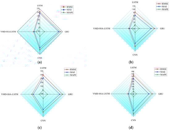
Figure 11.
Comparison Diagram of Model Evaluation Indicators for Spring (a), Comparison Diagram of Model Evaluation Indicators for Summer (b), Comparison Diagram of Model Evaluation Indicators for Autumn (c), Comparison Diagram of Model Evaluation Indicators for Winter (d).
As evidenced by the analysis in Table 5, the VMD-SSA-LSTM method consistently achieves the lowest RMSE, MAE, and MAPE values across all four seasons compared to the other three benchmark models. This robust performance unequivocally demonstrates the model’s superiority in heat load forecasting, which stems from its unique synergistic integration of adaptive signal decomposition (VMD), intelligent hyperparameter optimization (SSA), and long-term dependency modeling (LSTM)—capabilities that collectively address the nonlinearity, nonstationary, and multi-scale characteristics inherent in heat load data. Meanwhile, the analysis of the visualized radar charts in Figure 11 further confirms the superior prediction performance of the model proposed in this paper under different seasons, highlighting the potential of this model to provide more accurate and reliable predictions under different seasonal conditions. This is of great significance for the practical applications of energy management and the optimization of thermal systems.
5.2. Analysis of Ablation Experiments
5.2.1. Error Comparison
The thermal load data of the four seasons were input into three different models for ablation experiments. The LSTM model is the model obtained by removing the VMD and the SSA from the VMD-SSA-LSTM model proposed in this paper. The VMD-LSTM model is the model obtained by removing the SSA from the model of this paper. Finally, the error comparison diagram obtained from the experiment is shown in Figure 12.
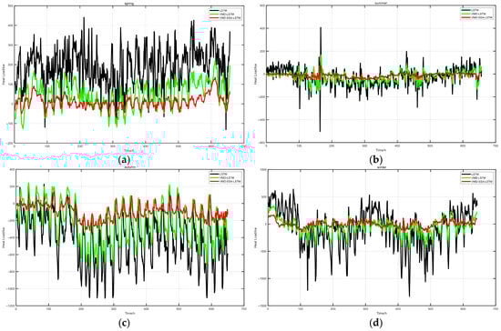
Figure 12.
Error Comparison Diagram of Three Models for Spring (a), Error Comparison Diagram of Three Models for Summer (b), Error Comparison Diagram of Three Models for Autumn (c), Error Comparison Diagram of Three Models for Winter (d).
In spring, as shown in Figure 12a, the VMD-SSA-LSTM model exhibits the lowest error. The curve is smooth with small fluctuations, which is significantly better than the LSTM and VMD-LSTM models, reflecting its advantage in dealing with transitional thermal load changes. In summer, as shown in Figure 12b, the VMD-SSA-LSTM model performs particularly outstandingly when dealing with high-frequency fluctuations. The error curve is stable and has a low amplitude, demonstrating good adaptability to complex changes in cooling demand. In autumn, as shown in Figure 12c, the VMD-SSA-LSTM model performs best in terms of capturing the transitional dynamics of thermal load from cooling to heating. The error curve is stable with small fluctuations, further verifying its effectiveness in handling nonlinear characteristics. In winter, as shown in Figure 12d, the VMD-SSA-LSTM model still maintains a low error level under the condition of extreme heating demand, demonstrating its robustness in dealing with high-amplitude and low-frequency changes.
Overall, by combining SSA optimization and VMD, the VMD-SSA-LSTM model significantly improves the prediction accuracy and stability, making it an optimal choice for seasonal thermal load forecasting.
5.2.2. Comparison of Evaluation Indicators
In addition, in the field of thermal load forecasting, the accuracy and reliability of the model are of vital importance. The Root Mean Square Error (RMSE), Mean Absolute Error (MAE), and Mean Absolute Percentage Error (MAPE) are key indicators for measuring the performance of the model. The lower the values of these indicators, the better the prediction effect. Table 6 shows the specific values of RMSE, MAE, and MAPE of the three models, namely LSTM, VMD-LSTM, and VMD-SSA-LSTM, in thermal load forecasting in the four seasons of spring, summer, autumn, and winter. In order to more intuitively compare the performance of the three models, LSTM, VMD-LSTM, and VMD-SSA-LSTM, in different seasons, visual radar charts were drawn based on the previous data of RMSE, MAE, and MAPE in Table 6, as shown in Figure 13. In Table 6, the downward black arrow indicates that a lower value of this evaluation indicator is considered better, and the bold black number represents that the corresponding model has achieved the minimum value of this indicator in the current season.
Table 6.
Comparison of Error Indicators.
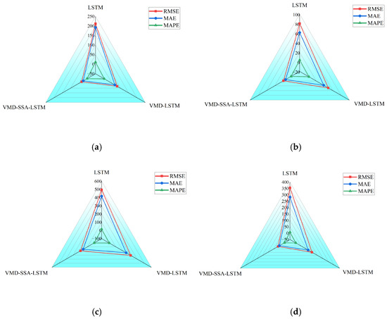
Figure 13.
Comparison of ablation experiment models for spring evaluation results (a), comparison of ablation experiment models for summer evaluation results (b), Comparison of ablation experiment models for autumn evaluation results (c), Comparison of ablation experiment models for winter evaluation results (d).
According to Table 6, under different seasons, the VMD-SSA-LSTM model demonstrates the best performance in these three indicators, significantly outperforming the LSTM and VMD-LSTM models. It effectively reduces various error indicators and shows higher prediction accuracy. The VMD-LSTM model also performs better than the LSTM model to a certain extent, which indicates that the VMD has a positive effect on the preprocessing of thermal load data. Moreover, the introduction of the SSA further optimizes the VMD-LSTM model, providing a more reliable method for accurate thermal load prediction. Analyzing Figure 13, Figure 13a represents spring, Figure 13b represents summer, Figure 13c represents autumn, and Figure 13d represents winter. In the figures, the red line represents RMSE, the blue line represents MAE, and the green line represents MAPE. The three axes correspond to the three models, namely LSTM, VMD-LSTM, and VMD-SSA-LSTM, respectively. Through intuitive graphical displays, these radar charts clearly reflect that in different seasons, compared with the LSTM and VMD-LSTM models, the VMD-SSA-LSTM model has smaller values in terms of the RMSE, MAE, and MAPE indicators, that is, lower errors, and shows better prediction performance. This strongly supports the effectiveness and dominant position of the VMD-SSA-LSTM model in thermal load forecasting.
5.2.3. Comparison of Prediction Results
For the thermal load data of the four seasons, the above three models were, respectively, used for prediction. The prediction results obtained by different models are shown in Figure 14. Among them, the black curve represents the actual thermal load data, the yellow curve represents the prediction fitting curve of the LSTM model, the green curve represents the prediction result of the VMD-LSTM model, and the red curve represents the prediction result of the VMD-SSA-LSTM model.
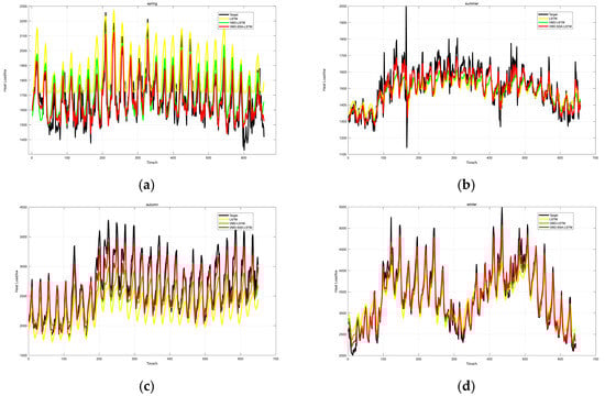
Figure 14.
Comparison Diagram of Prediction Results for Spring (a), Comparison Diagram of Prediction Results for Summer (b), Comparison Diagram of Prediction Results for Autumn (c), Comparison Diagram of Prediction Results for Winter (d).
Looking at the horizontal axis in Figure 14, it represents the number of samples, increasing from 0, which reflects the prediction situations of different models at each sample point. The vertical axis represents the thermal load power (in kW), showing the values of the actual thermal load and the predicted thermal loads of each model.
In the comparison diagram of spring predictions as shown in Figure 14a, the black actual thermal load curve fluctuates frequently and with large amplitudes, reflecting the complexity of thermal load changes in spring. Although the prediction curve of the LSTM model can roughly follow the trend of the actual curve, there are obvious deviations at some sample points, especially in areas where the thermal load fluctuates greatly, indicating that the LSTM model has certain limitations in terms of capturing the rapid changes in spring thermal load. The prediction curve of the VMD-LSTM model is improved to some extent compared with the LSTM model, and its degree of fitting with the actual curve has increased, being able to better reflect the fluctuation of the thermal load. However, there are still deviations at some peak and valley values. The red prediction curve of the VMD-SSA-LSTM model performs the most outstandingly, being able to closely fit the actual thermal load curve and accurately predict the changes in the thermal load at most sample points, reflecting the high precision of this model in terms of spring thermal load prediction.
In the comparison diagram of summer predictions as shown in Figure 14b, the fluctuations of the actual thermal load (the black curve) are relatively gentle, but there are still certain undulations. The prediction results of the LSTM model (the yellow curve) have large deviations from the actual values in some areas, especially at the turning points where the thermal load rises and falls, indicating that this model has deficiencies in dealing with the dynamic changes in the summer thermal load. The prediction performance of the VMD-LSTM model (the green curve) is improved, being able to more accurately capture the change trend of the thermal load, but there are still differences from the actual values in some details. The VMD-SSA-LSTM model (the red curve), however, once again demonstrates good performance. Its prediction curve highly coincides with the actual thermal load curve, and it performs very accurately both in grasping the trend and in predicting specific values, showing the effectiveness of this model in summer thermal load prediction.
In the comparison diagram of autumn predictions as shown in Figure 14c, the fluctuation of the actual thermal load is quite complex, presenting multiple peaks and valleys. The prediction results of the LSTM model have a certain correlation with the actual values in the overall trend, but there are large errors in specific values, especially in areas where the thermal load fluctuates violently. The prediction effect of the VMD-LSTM model is improved, being able to better follow the changes in the actual thermal load, but there is still a certain lag at some key fluctuation points. The prediction performance of the VMD-SSA-LSTM model is still outstanding, being able to closely follow the changes in the actual thermal load curve and accurately predict the peaks and valleys of the thermal load, reflecting the superiority of this model in dealing with complex thermal load changes.
In the comparison diagram of winter predictions as shown in Figure 14d, the actual thermal load shows obvious upward and downward trends, and the fluctuation amplitude is large. The prediction results of the LSTM model have a certain deviation from the actual values in the overall trend, especially in the rising stage of the thermal load, where the predicted values are significantly lower than the actual values. The prediction effect of the VMD-LSTM model is improved, being able to better reflect the change trend of the thermal load, but there are still gaps from the actual values in some details. The prediction curve of the VMD-SSA-LSTM model is the closest to the actual thermal load curve, being able to accurately capture the change trend and numerical values of the thermal load, showing high reliability in winter thermal load prediction.
In conclusion, the model in this paper was subjected to ablation experiments with seasonal adjustments. By comparing and analyzing the prediction results obtained from the experiments, it can clearly be seen that in terms of thermal load prediction for different seasons, compared with the LSTM model and the VMD-LSTM model, the VMD-SSA-LSTM model can more accurately fit the actual thermal load data, demonstrating better prediction performance and adaptability, and providing strong support for the accurate prediction of thermal load.
6. Conclusions
This paper proposes a short-term thermal load forecasting model of VMD-LSTM optimized by the Sparrow Search Algorithm (SSA). The dataset used is the public dataset of the integrated energy system from Arizona State University in the United States and the meteorological data of the corresponding period in this region. Multiple seasonal experiments have been conducted on the historical data of this dataset. According to the experimental data, the model proposed in this paper has the best performance in terms of the three indicators of RMSE, MAE, and MAPE under the four seasonal conditions of spring, summer, autumn, and winter. Judging from the data presented in the experimental results and discussions in the previous chapter, it further demonstrates the superiority of the model proposed in this paper.
In summary, through the above experiments, the following research achievements are obtained in this paper:
- Combining the advantages of the VMD algorithm in signal decomposition and the advantages of the LSTM model in time series prediction provides a new idea for the prediction of nonstationary thermal loads.
- The SSA is used to optimize the hyperparameters of the LSTM model, avoiding the blindness and computational complexity of the traditional grid search method, and improving the prediction accuracy and efficiency of the model.
- This combined model is particularly suitable for dealing with thermal load forecasting problems with strong seasonal and nonlinear characteristics, and can provide more reliable forecasting results for energy management and the optimization of the heating system.
In conclusion, the thermal load changes significantly with the seasons, and the accuracy of thermal load forecasting directly affects the operation efficiency of energy scheduling and the heating system. Through the seasonal adjustment, SSA optimization of hyperparameters, VMD, and LSTM prediction, the prediction accuracy can be significantly improved. It can not only solve the technical problems in thermal load forecasting but also has important practical application value, providing strong support for energy management and the optimization of the heating system.
From an engineering implementation perspective, the SSA demonstrates significant potential for practical deployment in real-world thermal load forecasting within energy systems. Specifically, the SSA features relatively few parameters and low sensitivity to initial parameter settings. These characteristics enable engineers to achieve satisfactory optimization results without extensive parameter tuning during deployment. Even across diverse application scenarios, adapting to new requirements merely involves straightforward parameter adjustments, thereby reducing the technical threshold for maintenance and operation. Future research will continue to focus on optimizing the SSA’s adaptability across various deployment environments (e.g., cloud–edge collaboration) to further validate its performance in complex scenarios.
Author Contributions
Methodology, K.H. and M.F.; Software, Y.Z.; Validation, Y.Z.; Formal analysis, L.L.; Investigation, L.L.; Resources, L.L.; Data curation, Q.Y.; Writing—original draft, Y.Z.; Writing—review & editing, K.H.; Visualization, Q.Y.; Supervision, M.F.; Project administration, M.F.; Funding acquisition, K.H. All authors have read and agreed to the published version of the manuscript.
Funding
This research was supported by the Baima Lake Laboratory Joint Fund of the Zhejiang Provincial Natural Science Foundation of China (Grant No. LBMHY25E060007), the Education Science Planning Project of Zhejiang Province, China (Grant No. 2024SCG026), the Collaborative Education Project of the Ministry of Education, China (Grant No. 231004994121114), the Teaching Construction and Reform Project (2024) at Hangzhou Normal University, China (Research on Smart Teaching Reform Based on Digital Twins), and the “Artificial Intelligence+” Course Construction Project (2025) at Hangzhou Normal University, China (Digital Twin Technology and Applications).
Data Availability Statement
The original contributions presented in this study are included in the article. Further inquiries can be directed to the corresponding author.
Conflicts of Interest
The authors declare that there are no conflicts of interest regarding the publication of this paper.
References
- Saloux, E.; Candanedo, J.A. Sizing and control optimization of thermal energy storage in a solar district heating system. Energy Rep. 2021, 7, 389–400. [Google Scholar] [CrossRef]
- Xiong, J.; Ye, Y.; Wang, Q.; Dong, X.; Lu, T.; Ma, D. A comprehensive review on distributed energy cooperative control and optimization method for energy interconnection system. Electr. Power Syst. Res. 2024, 237, 111007. [Google Scholar] [CrossRef]
- Idowu, S.; Saguna, S.; Åhlund, C.; Schelén, O. Applied machine learning: Forecasting heat load in district heating system. Energy Build. 2016, 133, 478–488. [Google Scholar] [CrossRef]
- Dahl, M.; Brun, A.; Andresen, G.B. Using ensemble weather predictions in district heating operation and load forecasting. Appl. Energy 2017, 193, 455–465. [Google Scholar] [CrossRef]
- Fang, T.; Lahdelma, R. Evaluation of a multiple linear regression model and SARIMA model in forecasting heat demand for district heating system. Appl. Energy 2016, 179, 544–552. [Google Scholar] [CrossRef]
- Wang, T.; Ma, T.; Yan, D.; Song, J.; Hu, J.; Zhang, G.; Zhuang, Y. Prediction of heating load fluctuation based on fuzzy information granulation and support vector machine. Therm. Sci. 2021, 25, 3219–3228. [Google Scholar] [CrossRef]
- Olu-Ajayi, R.; Alaka, H.; Sulaimon, I.; Sunmola, F.; Ajayi, S. Building energy consumption prediction for residential buildings using deep learning and other machine learning techniques. J. Build. Eng. 2022, 45, 103406. [Google Scholar] [CrossRef]
- Wei, Z.; Zhang, T.; Yue, B.; Ding, Y.; Xiao, R.; Wang, R.; Zhai, X. Prediction of residential district heating load based on machine learning: A case study. Energy 2021, 231, 120950. [Google Scholar] [CrossRef]
- Kurek, T.; Bielecki, A.; Świrski, K.; Wojdan, K.; Guzek, M.; Białek, J.; Brzozowski, R.; Serafin, R. Heat demand forecasting algorithm for a Warsaw district heating network. Energy 2021, 217, 119347. [Google Scholar] [CrossRef]
- Koschwitz, D.; Frisch, J.; Van Treeck, C. Data-driven heating and cooling load predictions for non-residential buildings based on support vector machine regression and NARX Recurrent Neural Network: A comparative study on district scale. Energy 2018, 165, 134–142. [Google Scholar] [CrossRef]
- He, N.; Zhang, L.; Qian, C.; Gao, F.; Li, R.; Cheng, F.; Chu, D. Short-term cooling load prediction for central air conditioning systems with small sample based on permutation entropy and temporal convolutional network. Energy Build. 2024, 310, 114115. [Google Scholar] [CrossRef]
- Zhang, Z.; Tian, Z.; Wu, Z.; Xu, B. Development and analysis of a BP-LSTM-Kriging temperature field prediction model for the arch ring section of the reinforced concrete arch bridge. Structures 2024, 64, 106564. [Google Scholar] [CrossRef]
- Lv, R.; Yuan, Z.; Lei, B.; Zheng, J.; Luo, X. Building thermal load prediction using deep learning method considering time-shifting correlation in feature variables. J. Build. Eng. 2022, 61, 105316. [Google Scholar] [CrossRef]
- Wang, Z.; Hong, T.; Piette, M.A. Building thermal load prediction through shallow machine learning and deep learning. Appl. Energy 2020, 263, 114683. [Google Scholar] [CrossRef]
- Wang, M.; Tian, Q. Dynamic heat supply prediction using support vector regression optimized by particle swarm optimization algorithm. Math. Probl. Eng. 2016, 2016, 3968324. [Google Scholar] [CrossRef]
- Yan, Q.; Lu, Z.; Liu, H.; He, X.; Zhang, X.; Guo, J. An improved feature-time Transformer encoder-Bi-LSTM for short-term forecasting of user-level integrated energy loads. Energy Build. 2023, 297, 113396. [Google Scholar] [CrossRef]
- Gao, Z.; Yang, S.; Yu, J.; Zhao, A. Hybrid forecasting model of building cooling load based on combined neural network. Energy 2024, 297, 131317. [Google Scholar] [CrossRef]
- Bo, Y.; Guo, X.; Liu, Q.; Pan, Y.; Zhang, L.; Lu, Y. Prediction of tunnel deformation using PSO variant integrated with XGBoost and its TBM jamming application. Tunn. Undergr. Space Technol. 2024, 150, 105842. [Google Scholar] [CrossRef]
- Li, H.; Li, S.; Sun, J.; Huang, B.; Zhang, J.; Gao, M. Ultrasound signal processing based on joint GWO-VMD wavelet threshold functions. Measurement 2024, 226, 114143. [Google Scholar] [CrossRef]
- Tang, Y.; Dai, Q.; Yang, M.; Du, T.; Chen, L. Software defect prediction ensemble learning algorithm based on adaptive variable sparrow search algorithm. Int. J. Mach. Learn. Cybern. 2023, 14, 1967–1987. [Google Scholar] [CrossRef]
- Yan, P.; Shang, S.; Zhang, C.; Yin, N.; Zhang, X.; Yang, G.; Zhang, Z.; Sun, Q. Research on the processing of coal mine water source data by optimizing BP neural network algorithm with sparrow search algorithm. IEEE Access 2021, 9, 108718–108730. [Google Scholar] [CrossRef]
- Ribeiro, G.T.; Mariani, V.C.; dos Santos Coelho, L. Enhanced ensemble structures using wavelet neural networks applied to short-term load forecasting. Eng. Appl. Artif. Intell. 2019, 82, 272–281. [Google Scholar] [CrossRef]
- Chen, L.; Tian, Z.; Zhou, S.; Gong, Q.; Di, H. Attitude deviation prediction of shield tunneling machine using time-aware LSTM networks. Transp. Geotech. 2024, 45, 101195. [Google Scholar] [CrossRef]
- Mounir, N.; Ouadi, H.; Jrhilifa, I. Short-term electric load forecasting using an EMD-BI-LSTM approach for smart grid energy management system. Energy Build. 2023, 288, 113022. [Google Scholar] [CrossRef]
- Ma, Q.; Ye, R. Short-Term Prediction of the Intermediate Point Temperature of a Supercritical Unit Based on the EEMD–LSTM Method. Energies 2024, 17, 949. [Google Scholar] [CrossRef]
- Lei, W.; Wang, G.; Wan, B.; Min, Y.; Wu, J.; Li, B. High voltage shunt reactor acoustic signal denoising based on the combination of VMD parameters optimized by coati optimization algorithm and wavelet threshold. Measurement 2024, 224, 113854. [Google Scholar] [CrossRef]
- Fang, M.; Zhang, F.; Yang, Y.; Tao, R.; Xiao, R.; Zhu, D. The influence of optimization algorithm on the signal prediction accuracy of VMD-LSTM for the pumped storage hydropower unit. J. Energy Storage 2024, 78, 110187. [Google Scholar] [CrossRef]
- Yao, X.; Liu, Y.; Lin, G. Evolutionary programming made faster. IEEE Trans. Evol. Comput. 1999, 3, 82–102. [Google Scholar] [CrossRef]
- Tan, M.; Liao, C.; Chen, J.; Cao, Y.; Wang, R.; Su, Y. A multi-task learning method for multi-energy load forecasting based on synthesis correlation analysis and load participation factor. Appl. Energy 2023, 343, 121177. [Google Scholar] [CrossRef]
- NSRDB Data Viewer. Available online: https://maps.nrel.gov/nsrdb-viewer (accessed on 17 November 2024).
Disclaimer/Publisher’s Note: The statements, opinions and data contained in all publications are solely those of the individual author(s) and contributor(s) and not of MDPI and/or the editor(s). MDPI and/or the editor(s) disclaim responsibility for any injury to people or property resulting from any ideas, methods, instructions or products referred to in the content. |
© 2025 by the authors. Licensee MDPI, Basel, Switzerland. This article is an open access article distributed under the terms and conditions of the Creative Commons Attribution (CC BY) license (https://creativecommons.org/licenses/by/4.0/).