


A Hybrid LMD–ARIMA–Machine Learning Framework for Enhanced Forecasting of Financial Time Series: Evidence from the NASDAQ Composite Index

 ,
,  ,
,  ,
,  ,
,  and
and
Abstract
1. Introduction
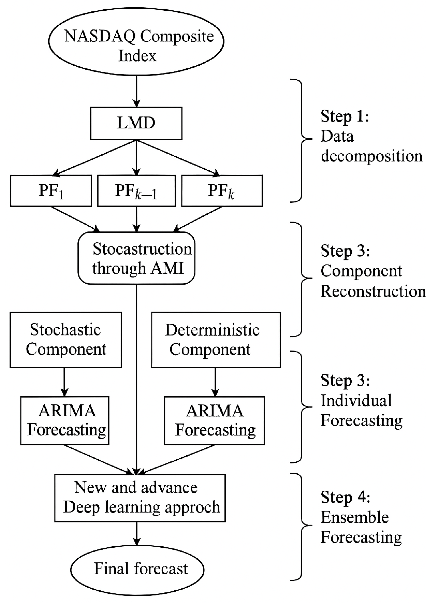
2. Methodology
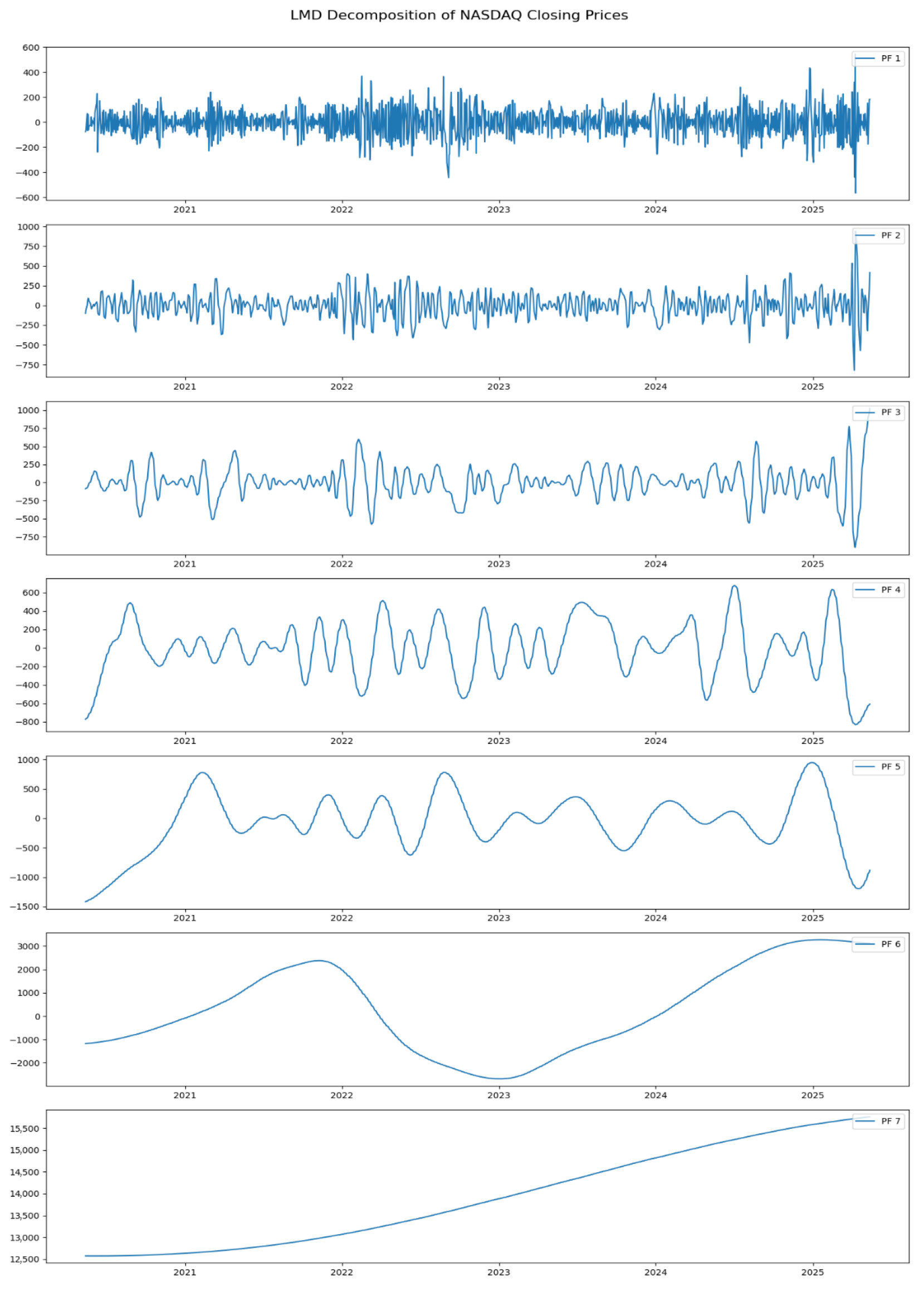
2.1. Local Mean Decomposition (LMD)
- Identify all local extrema . Compute local mean and local envelope estimate , as follows:
- Smooth and using moving average filters to obtain and .
- Obtain the zero-mean signal, as follows:
- Normalize using the envelope, as follows:
- Repeat the demodulation iteratively to obtain the following:
- Construct the first product function, as follows:
2.2. Autoregressive Integrated Moving Average
2.3. Random Forest
- Bootstrap Aggregation (Bagging): Each decision tree is trained on a bootstrapped subset of the training data.
- Feature Randomness: At each split in a tree, a random subset of features is considered instead of the full set.
2.4. Artificial Neural Network
2.5. Support Vector Machine
- Linear: ;
- Polynomial: ;
- RBF: .
2.6. XGBoost
2.7. Evaluation Metrics
2.8. Diebold–Mariano Test
2.9. Directional Statistic
3. Empirical Analysis
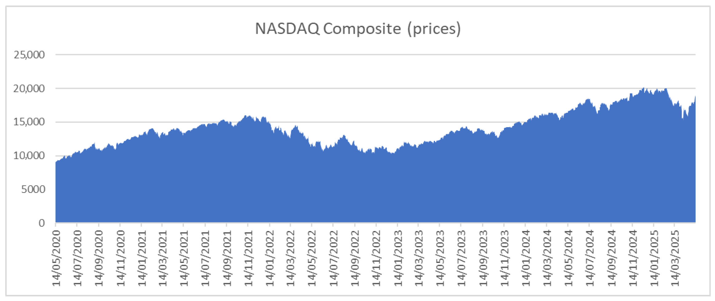
3.1. Statistical Analysis of the Data
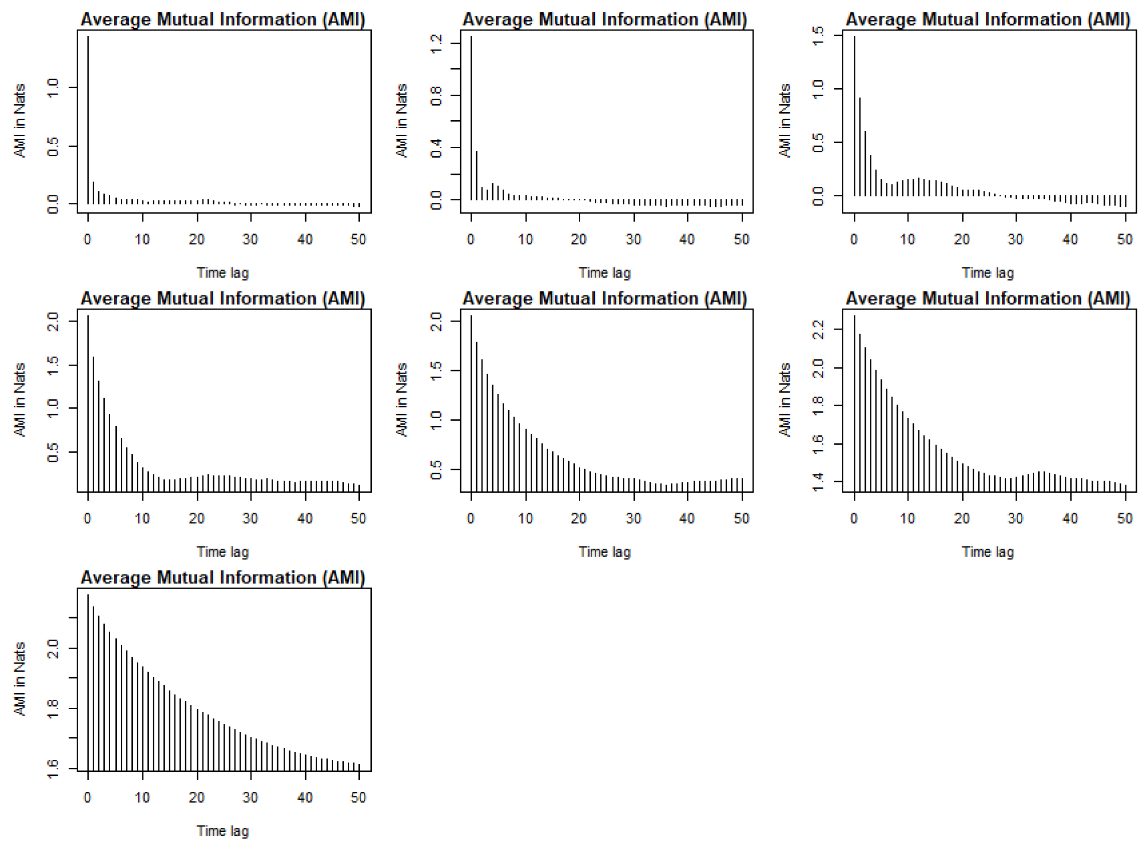
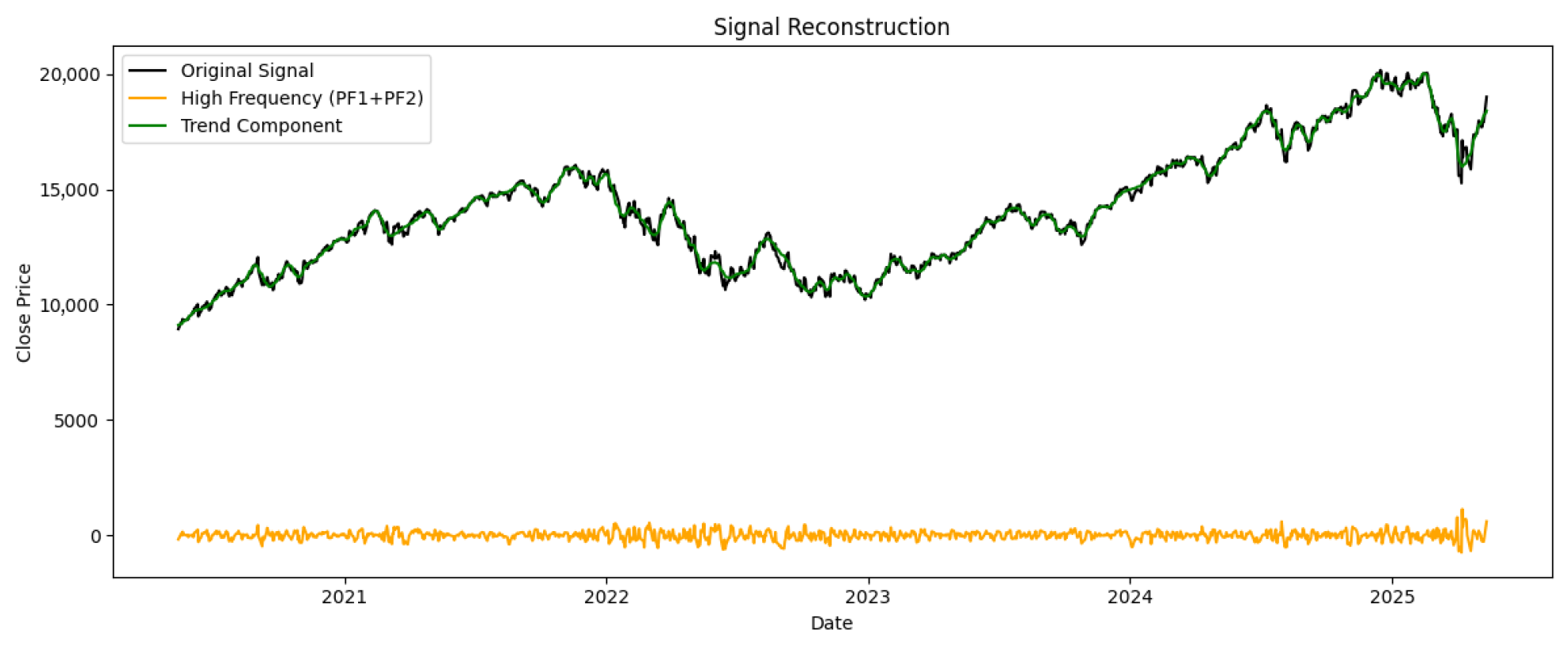
3.2. Data Decomposition and Reconstruction
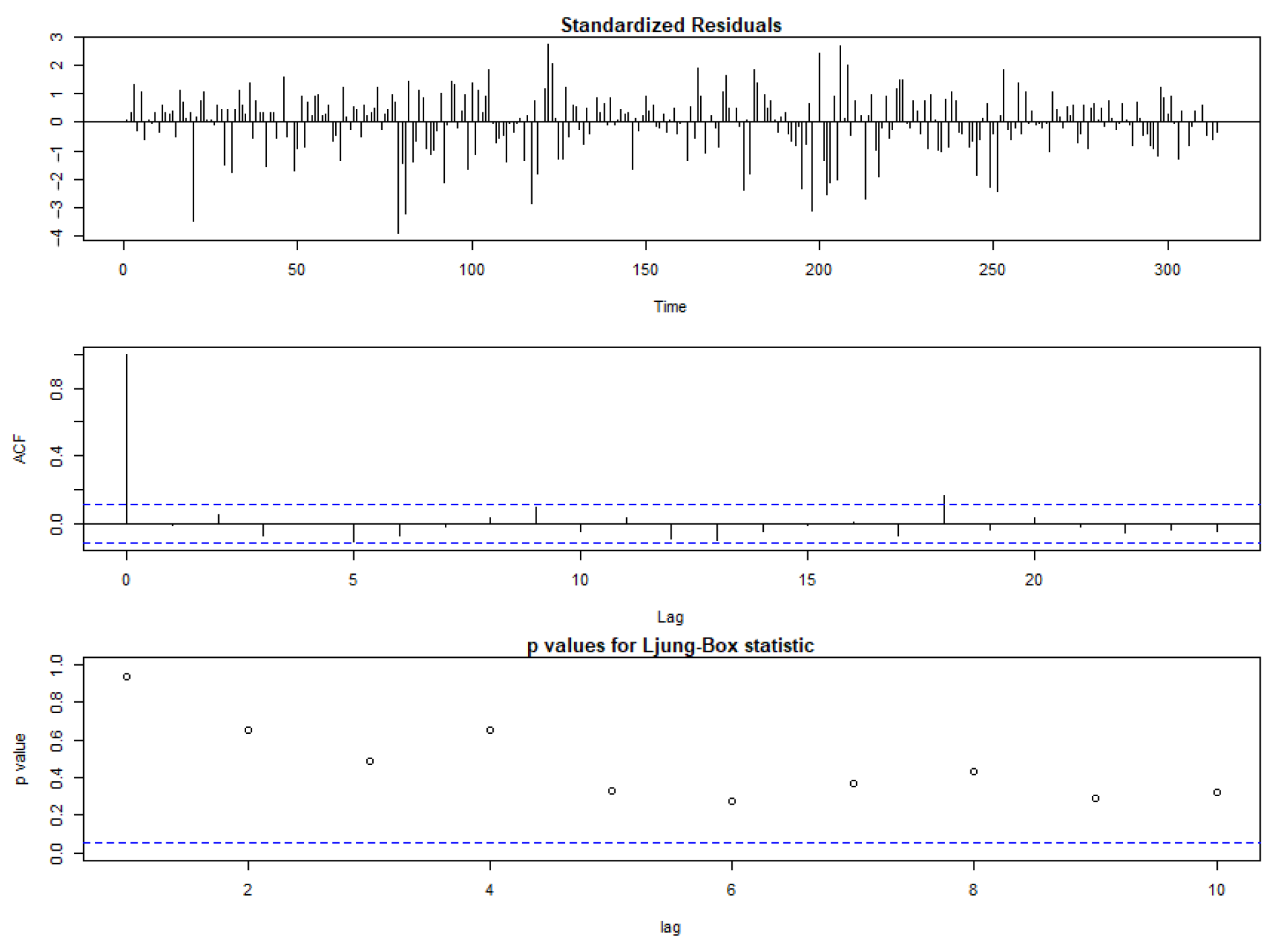
3.3. Stochastic and Deterministic Modeling Using ARIMA
3.4. Machine Learning Analysis
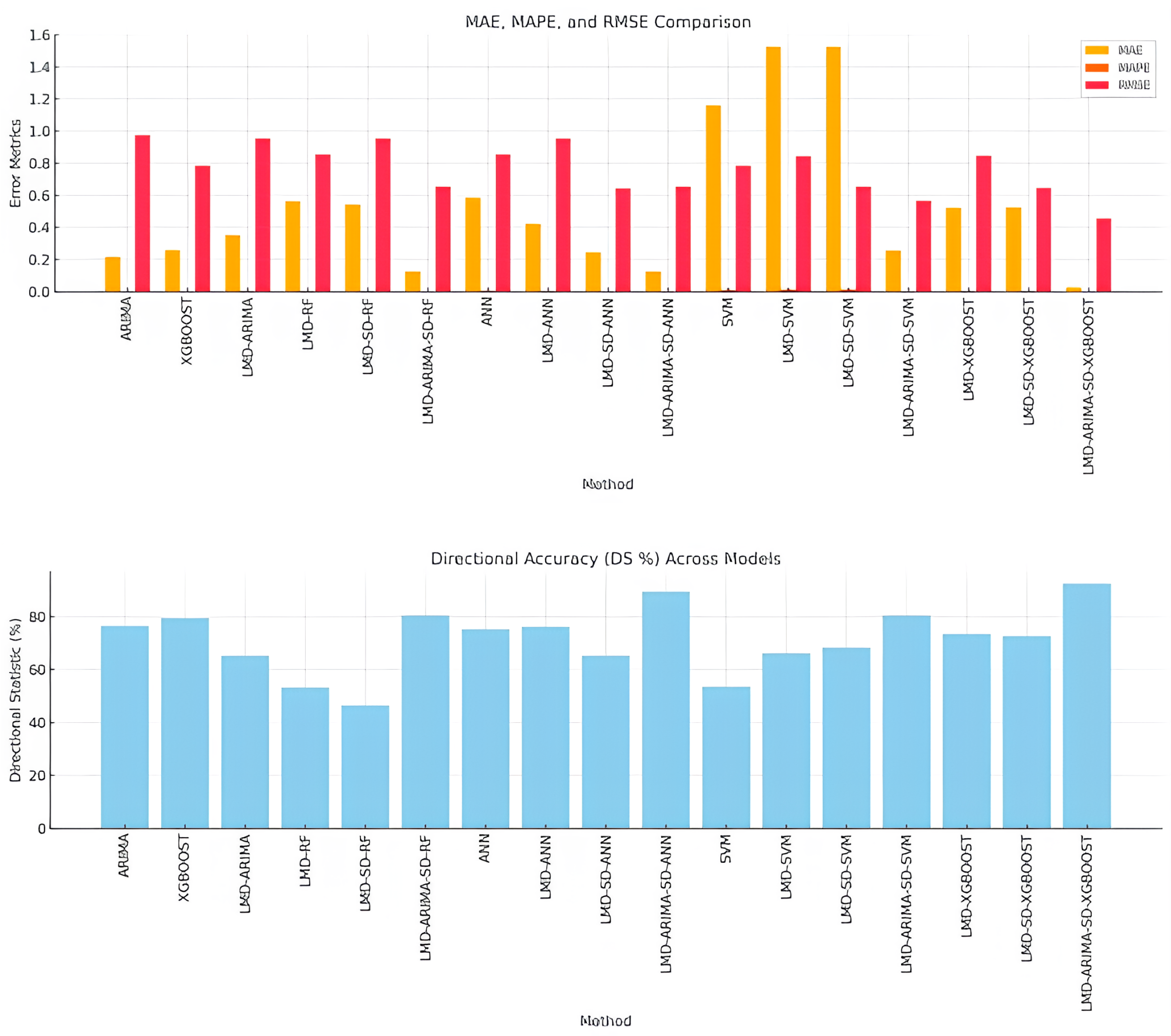
3.5. Outcomes and Discussion
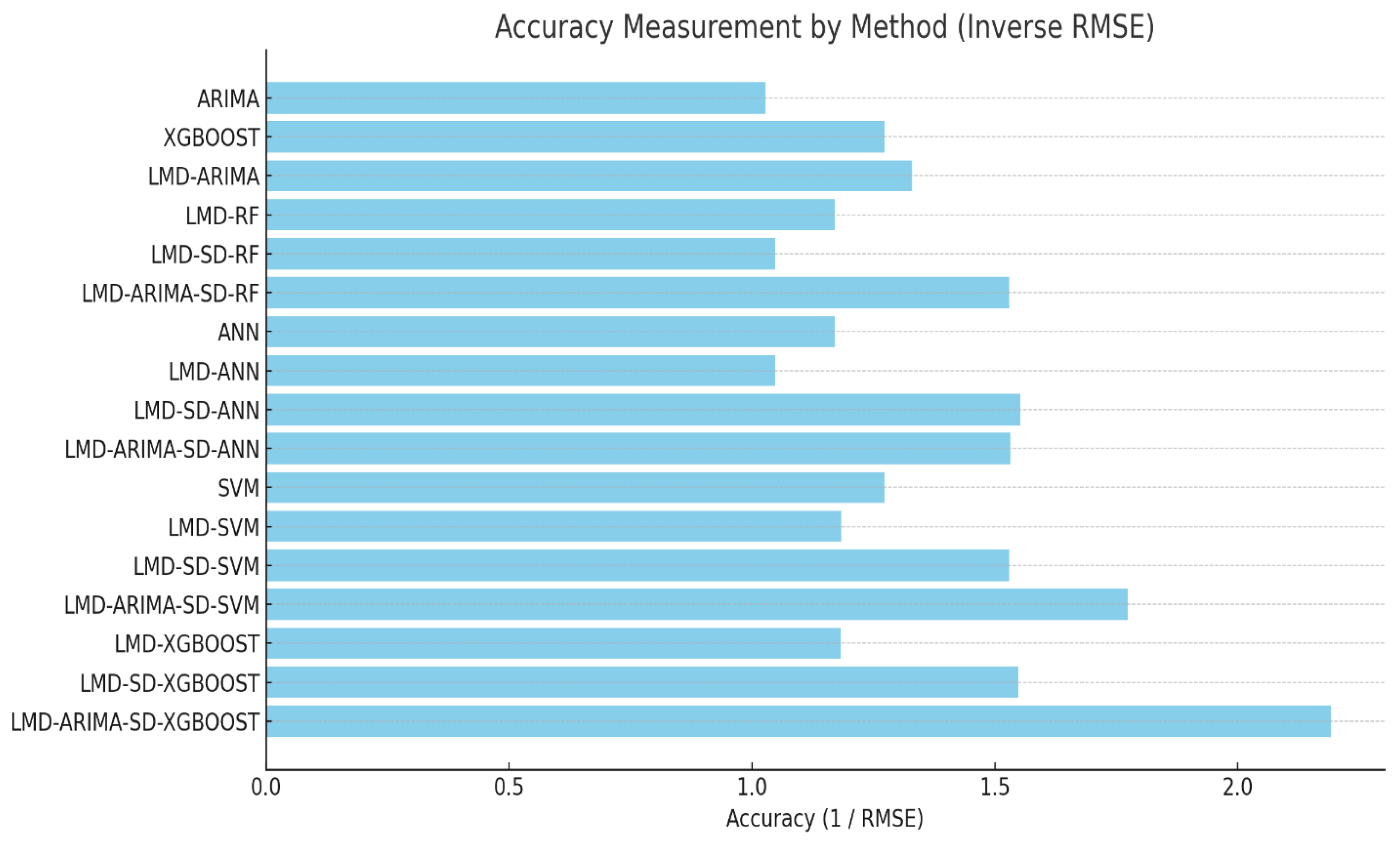
3.6. Performance Summary and Model Comparison
4. Conclusions and Future Work
Author Contributions
Funding
Data Availability Statement
Acknowledgments
Conflicts of Interest
References
- Zhang, Y.; Zhou, D. Volatility forecasting of NASDAQ composite index using GARCH models. J. Financ. Mark. 2020, 25, 321–336. [Google Scholar]
- Dong, X.; Yu, M. Time-varying effects of macro shocks on cross-border capital flows in China’s bond market. Int. Rev. Econ. Financ. 2024, 96, 103720. [Google Scholar] [CrossRef]
- Chatrath, A.; Christie-David, R.; Ramchander, S. Time-varying risk premia in the futures markets: Evidence from the S&P 500 and NASDAQ 100 indexes. J. Financ. Res. 1995, 18, 381–395. [Google Scholar]
- Li, H.; Xia, C.; Wang, T.; Wang, Z.; Cui, P.; Li, X. GRASS: Learning Spatial-Temporal Properties From Chainlike Cascade Data for Microscopic Diffusion Prediction. IEEE Trans. Neural Netw. Learn. Syst. 2024, 35, 16313–16327. [Google Scholar] [CrossRef] [PubMed]
- Dong, X.; Yu, M. Green bond issuance and green innovation: Evidence from China’s energy industry. Int. Rev. Financ. Anal. 2024, 94, 103281. [Google Scholar] [CrossRef]
- Ifleh, A.; El Kabbouri, M. Stock price indices prediction combining deep learning algorithms and selected technical indicators based on correlation. Arab Gulf J. Sci. Res. 2024, 42, 1237–1256. [Google Scholar] [CrossRef]
- Lin, C.Y.; Marques, J.A.L. Stock market prediction using artificial intelligence: A systematic review of systematic reviews. Soc. Sci. Humanit. Open 2024, 9, 100864. [Google Scholar] [CrossRef]
- Alam, K.; Bhuiyan, M.H.; Ul Haque, I.; Monir, M.F.; Ahmed, T. Enhancing stock market prediction: A robust LSTM-DNN model analysis on 26 real-life datasets. IEEE Access 2024, 12, 122757–122768. [Google Scholar] [CrossRef]
- Smith, J.S. The local mean decomposition and its application to EEG signal processing. Biomed. Signal Process. Control 2005, 1, 1–8. [Google Scholar]
- Huang, N.E.; Shen, Z.; Long, S.R.; Wu, M.C.; Shih, H.H.; Zheng, Q.; Yen, N.C.; Tung, C.C.; Liu, H.H. The empirical mode decomposition and the Hilbert spectrum for nonlinear and non-stationary time series analysis. Proc. R. Soc. A 2007, 454, 903–995. [Google Scholar] [CrossRef]
- Khan, F.; Iftikhar, H.; Khan, I.; Rodrigues, P.C.; Alharbi, A.A.; Allohibi, J. A Hybrid Vector Autoregressive Model for Accurate Macroeconomic Forecasting: An Application to the US Economy. Mathematics 2025, 13, 1706. [Google Scholar] [CrossRef]
- Zhang, Q.; Liu, G.; Yang, Y. Application of local mean decomposition and permutation entropy in fault diagnosis. Mech. Syst. Signal Process. 2018, 101, 404–415. [Google Scholar]
- Fischer, T.; Krauss, C. Deep learning with long short-term memory networks for financial market predictions. Eur. J. Oper. Res. 2018, 270, 654–669. [Google Scholar] [CrossRef]
- Chong, E.; Han, C.; Park, F.C. Deep learning networks for stock market analysis and prediction. Expert Syst. Appl. 2017, 83, 187–205. [Google Scholar] [CrossRef]
- Patel, J.; Shah, S.; Thakkar, P.; Kotecha, K. Predicting stock market index using fusion of machine learning techniques. Expert Syst. Appl. 2015, 42, 2162–2172. [Google Scholar] [CrossRef]
- Iftikhar, H.; Khan, M.; Turpo-Chaparro, J.E.; Rodrigues, P.C.; López-Gonzales, J.L. Forecasting stock prices using a novel filtering-combination technique: Application to the Pakistan stock exchange. AIMS Math. 2024, 9, 3264–3288. [Google Scholar] [CrossRef]
- Xiong, W.; He, D.; Du, H. Learning economic model predictive control via clustering and kernel-based Lipschitz regression. J. Frankl. Inst. 2025, 362, 107787. [Google Scholar] [CrossRef]
- Luo, J.; Zhuo, W.; Xu, B. A Deep Neural Network-Based Assistive Decision Method for Financial Risk Prediction in Carbon Trading Market. J. Circuits Syst. Comput. 2023, 33, 2450153. [Google Scholar] [CrossRef]
- Kim, H.; Shin, K. A hybrid approach using neural networks and genetic algorithms for temporal patterns in stock markets. Appl. Soft Comput. 2007, 7, 569–576. [Google Scholar] [CrossRef]
- Zhang, X.; Yang, X.; He, Q. Multi-scale systemic risk and spillover networks of commodity markets in the bullish and bearish regimes. N. Am. J. Econ. Financ. 2022, 62, 101766. [Google Scholar] [CrossRef]
- Yang, R.; Li, H.; Huang, H. Multisource information fusion considering the weight of focal element’s beliefs: A Gaussian kernel similarity approach. Meas. Sci. Technol. 2024, 35, 025136. [Google Scholar] [CrossRef]
- Kanniainen, K.; Pölönen, S.P.; Manner, A. Stock return prediction with LSTM neural networks: An evaluation using a multiple testing framework. Quant. Financ. 2021, 21, 1119–1134. [Google Scholar]
- Iftikhar, H.; Khan, F.; Rodrigues, P.C.; Alharbi, A.A.; Allohibi, J. Forecasting of Inflation Based on Univariate and Multivariate Time Series Models: An Empirical Application. Mathematics 2025, 13, 1121. [Google Scholar] [CrossRef]
- Quah, T.E.F.; Srinivasan, B. Improving returns using neural networks and genetic algorithms. Expert Syst. Appl. 2005, 29, 317–330. [Google Scholar]
- Huang, Y.; Liu, Y.; Lin, M. A fault diagnosis method based on LMD and SVM for roller bearings. Shock Vib. 2016, 2016, 1–11. [Google Scholar]
- Yan, R.; Gao, R.X.; Chen, X. Wavelets for fault diagnosis of rotary machines: A review. Signal Process. 2014, 96, 1–15. [Google Scholar] [CrossRef]
- Zhang, H.; Meng, G.; Qin, M. Bearing fault diagnosis based on local mean decomposition and generalized discriminant analysis. J. Mech. Sci. Technol. 2013, 27, 173–180. [Google Scholar]
- Krauss, C.; Do, X.A.; Huck, N. Deep neural network, gradient-boosted trees, random forests: Statistical arbitrage on the S & P 500. Eur. J. Oper. Res. 2017, 259, 689–702. [Google Scholar]
- Bao, W.; Yue, J.; Rao, Y. A deep learning framework for financial time series using stacked autoencoders and LSTM. PLoS ONE 2017, 12, e0180944. [Google Scholar] [CrossRef] [PubMed]
- Sirignano, P.; Cont, R. Universal features of price formation in financial markets. Quant. Financ. 2019, 19, 1449–1459. [Google Scholar] [CrossRef]
- Yang, X.; Chen, J.; Li, D.; Li, R. Functional-Coefficient Quantile Regression for Panel Data with Latent Group Structure. J. Bus. Econ. Stat. 2024, 42, 1026–1040. [Google Scholar] [CrossRef] [PubMed]
- Qureshi, M.; Iftikhar, H.; Rodrigues, P.C.; Rehman, M.Z.; Salar, S.A. Statistical modeling to improve time series forecasting using machine learning, time series, and hybrid models: A case study of bitcoin price forecasting. Mathematics 2024, 12, 3666. [Google Scholar] [CrossRef]
- Xu, A.; Dai, Y.; Hu, Z.; Qiu, K. Can green finance policy promote inclusive green growth?–Based on the quasi-natural experiment of China’s green finance reform and innovation pilot zone. Int. Rev. Econ. Financ. 2025, 100, 104090. [Google Scholar] [CrossRef]
- Chen, A.Y. The predictability of stock returns: A review. Int. Rev. Econ. Financ. 2016, 43, 160–174. [Google Scholar]
- Kim, J.B.; Kim, Y.A.; Kim, S.A. Investor sentiment and stock market volatility: Evidence from the NASDAQ Index. Financ. Res. Lett. 2019, 30, 1–7. [Google Scholar]
- Iftikhar, H.; Khan, F.; Torres Armas, E.A.; Rodrigues, P.C.; López-Gonzales, J.L. A novel hybrid framework for forecasting stock indices based on the nonlinear time series models. Comput. Stat. 2025, 1–24. [Google Scholar] [CrossRef]
- Wahal, R.; Yavuz, A. Institutional trading and stock returns. J. Financ. Quant. Anal. 2013, 48, 103–123. [Google Scholar]
- Wang, J.; Chen, J.; Xiang, L. An improved local mean decomposition method and its application in bearing fault diagnosis. J. Vib. Control 2016, 22, 4311–4324. [Google Scholar]
- Duan, R.; He, Y.; Cheng, Y. Rolling element bearing fault diagnosis using local mean decomposition and improved multiscale permutation entropy. Entropy 2019, 21, 683. [Google Scholar]
- Wang, Y.; Yan, K. Machine learning-based quantitative trading strategies across different time intervals in the American market. Quant. Financ. Econ. 2023, 7, 569–594. [Google Scholar] [CrossRef]
- Box, G.E.P.; Jenkins, G.M. Time Series Analysis: Forecasting and Control, 1st ed.; Holden-Day: San Francisco, CA, USA, 1970. [Google Scholar]
- Breiman, L. Random Forests. Mach. Learn. 2001, 45, 5–32. [Google Scholar] [CrossRef]
- Shah, I.; Iftikhar, H.; Ali, S.; Wang, D. Short-term electricity demand forecasting using components estimation technique. Energies 2019, 12, 2532. [Google Scholar] [CrossRef]
- Zhang, X.; Liu, G. Stock Prices Forecasting by Using a Novel Hybrid Method Based on the MFO-Optimized GRU Network. Ann. Data Sci. 2025, 12, 1369–1387. [Google Scholar] [CrossRef]
- Iftikhar, H.; Zafar, A.; Turpo-Chaparro, J.E.; Canas Rodrigues, P.; López-Gonzales, J.L. Forecasting day-ahead brent crude oil prices using hybrid combinations of time series models. Mathematics 2023, 11, 3548. [Google Scholar] [CrossRef]
- Hamilton, J.D. Time Series Analysis; Princeton University Press: Princeton, NJ, USA, 1994. [Google Scholar]
- Box, G.E.P.; Jenkins, G.M.; Reinsel, G.C.; Ljung, G.M. Time Series Analysis: Forecasting and Control, 5th ed.; Wiley: Hoboken, NJ, USA, 2015. [Google Scholar]
- Dickey, D.A.; Fuller, W.A. Distribution of the estimators for autoregressive time series with a unit root. J. Am. Stat. Assoc. 1979, 74, 427–431. [Google Scholar] [CrossRef] [PubMed]


| Min. | 1st Qu. | Median | Mean | 3rd Qu. | Max. | ADF | PP | Jarque–Bera |
|---|---|---|---|---|---|---|---|---|
| 8944 | 11,903 | 13,772 | 14,103 | 15,798 | 20,174 | 0.6878 | 0.7324 |
| Test | PF1 | PF2 | SPF |
|---|---|---|---|
| ADF | −4.325 (0.535) * | −4.248 (0.575) * | −1.756 (0.635) * |
| PP | 6.526 (0.999) * | 6.854 (0.999) * | −6.524 (0.700) * |
| Component | ARIMA | MAE | MAPE | RMSE | AIC | L–B Test |
|---|---|---|---|---|---|---|
| PF1 | (1, 1, 1) | 0.0015 | 0.000015 | 0.356 | −145.62 | 0.5421 (0.003) * |
| PF2 | (1, 2, 2) | 0.0256 | 0.000256 | 0.343 | −165.342 | 0.35214 (0.02) * |
| SPF | (2, 2, 1) | 0.0352 | 0.000352 | 0.2556 | −752.132 | 0.5417 (0.003) * |
| Model | Key Hyperparameters |
|---|---|
| XGBoost | n_estimators = 300, max_depth = 5, learning_rate = 0.1, subsample = 0.8 |
| ANN | Two hidden layers (64 and 32 neurons); Activation: ReLU; Optimizer: Adam (learning rate = 0.001) |
| Random Forest | n_estimators = 100, max_depth = 7 |
| SVM | Kernel: RBF; C = 1; gamma = scale |
| Method | MAE | MAPE | RMSE | DS (%) |
|---|---|---|---|---|
| ARIMA | 0.2154 | 0.002154 | 0.973 | 76.54 |
| XGBOOST | 0.2561 | 0.002561 | 0.785 | 79.35 |
| LMD–ARIMA | 0.3514 | 0.003514 | 0.954 | 65.24 |
| LMD–RF | 0.5621 | 0.005621 | 0.854 | 53.24 |
| LMD–SD–RF | 0.5412 | 0.005412 | 0.954 | 46.52 |
| LMD–ARIMA–SD–RF | 0.1251 | 0.001251 | 0.654 | 80.53 |
| ANN | 0.5824 | 0.005824 | 0.854 | 75.21 |
| LMD–ANN | 0.4213 | 0.004213 | 0.954 | 76.21 |
| LMD–SD–ANN | 0.2451 | 0.002451 | 0.644 | 65.32 |
| LMD–ARIMA–SD–ANN | 0.1254 | 0.001254 | 0.653 | 89.54 |
| SVM | 1.1587 | 0.011587 | 0.785 | 53.52 |
| LMD–SVM | 1.5246 | 0.015246 | 0.845 | 66.21 |
| LMD–SD–SVM | 1.5241 | 0.015241 | 0.654 | 68.24 |
| LMD–ARIMA–SD–SVM | 0.2546 | 0.002546 | 0.564 | 80.54 |
| LMD–XGBOOST | 0.5214 | 0.005214 | 0.8457 | 73.52 |
| LMD–SD–XGBOOST | 0.5241 | 0.005241 | 0.6458 | 72.65 |
| LMD–ARIMA–SD–XGBOOST | 0.0254 | 0.000254 | 0.4562 | 92.51 |
| Model Category | Best Variant | Accuracy () | Remarks |
|---|---|---|---|
| Traditional Models | ARIMA | 1.028 | Serves as the baseline reference |
| Machine Learning Models | XGBoost (first entry) | 1.274 | Outperforms ANN and SVM variants |
| Hybrid LMD Models | LMD–ARIMA | 1.048–1.322 | Provides moderate accuracy improvements |
| LMD + SD Hybrid Models | LMD–ARIMA–SD-XGBoost | 2.192 | Achieves the best overall performance |
| ANN Variants | LMD–ARIMA–SD–ANN | 1.531 | High-performing neural network-based approach |
| SVM Variants | LMD–ARIMA–SD–SVM | 1.773 | Enhanced performance using SVM-based prediction |
Disclaimer/Publisher’s Note: The statements, opinions and data contained in all publications are solely those of the individual author(s) and contributor(s) and not of MDPI and/or the editor(s). MDPI and/or the editor(s) disclaim responsibility for any injury to people or property resulting from any ideas, methods, instructions or products referred to in the content. |
© 2025 by the authors. Licensee MDPI, Basel, Switzerland. This article is an open access article distributed under the terms and conditions of the Creative Commons Attribution (CC BY) license (https://creativecommons.org/licenses/by/4.0/).
Share and Cite
Nasir, J.; Iftikhar, H.; Aamir, M.; Iftikhar, H.; Rodrigues, P.C.; Rehman, M.Z. A Hybrid LMD–ARIMA–Machine Learning Framework for Enhanced Forecasting of Financial Time Series: Evidence from the NASDAQ Composite Index. Mathematics 2025, 13, 2389. https://doi.org/10.3390/math13152389
Nasir J, Iftikhar H, Aamir M, Iftikhar H, Rodrigues PC, Rehman MZ. A Hybrid LMD–ARIMA–Machine Learning Framework for Enhanced Forecasting of Financial Time Series: Evidence from the NASDAQ Composite Index. Mathematics. 2025; 13(15):2389. https://doi.org/10.3390/math13152389
Chicago/Turabian StyleNasir, Jawaria, Hasnain Iftikhar, Muhammad Aamir, Hasnain Iftikhar, Paulo Canas Rodrigues, and Mohd Ziaur Rehman. 2025. "A Hybrid LMD–ARIMA–Machine Learning Framework for Enhanced Forecasting of Financial Time Series: Evidence from the NASDAQ Composite Index" Mathematics 13, no. 15: 2389. https://doi.org/10.3390/math13152389
APA StyleNasir, J., Iftikhar, H., Aamir, M., Iftikhar, H., Rodrigues, P. C., & Rehman, M. Z. (2025). A Hybrid LMD–ARIMA–Machine Learning Framework for Enhanced Forecasting of Financial Time Series: Evidence from the NASDAQ Composite Index. Mathematics, 13(15), 2389. https://doi.org/10.3390/math13152389