An Omni-Dimensional Dynamic Convolutional Network for Single-Image Super-Resolution Tasks

Abstract

The goal of single-image super-resolution (SISR) tasks is to generate high-definition images from low-quality inputs, with practical uses spanning healthcare diagnostics, aerial imaging, and surveillance systems. Although cnns have considerably improved image reconstruction quality, existing methods still face limitations, including inadequate restoration of high-frequency details, high computational complexity, and insufficient adaptability to complex scenes. To address these challenges, we propose an Omni-dimensional Dynamic Convolutional Network (ODConvNet) tailored for SISR tasks. Specifically, ODConvNet comprises four key components: a Feature Extraction Block (FEB) that captures low-level spatial features; an Omni-dimensional Dynamic Convolution Block (DCB), which utilizes a multidimensional attention mechanism to dynamically reweight convolution kernels across spatial, channel, and kernel dimensions, thereby enhancing feature expressiveness and context modeling; a Deep Feature Extraction Block (DFEB) that stacks multiple convolutional layers with residual connections to progressively extract and fuse high-level features; and a Reconstruction Block (RB) that employs subpixel convolution to upscale features and refine the final HR output. This mechanism significantly enhances feature extraction and effectively captures rich contextual information. Additionally, we employ an improved residual network structure combined with a refined Charbonnier loss function to alleviate gradient vanishing and exploding to enhance the robustness of model training. Extensive experiments conducted on widely used benchmark datasets, including DIV2K, Set5, Set14, B100, and Urban100, demonstrate that, compared with existing deep learning-based SR methods, our ODConvNet method improves Peak Signal-to-Noise Ratio (PSNR) and Structural Similarity Index (SSIM), and the visual quality of SR images is also improved. Ablation studies further validate the effectiveness and contribution of each component in our network. The proposed ODConvNet offers an effective, flexible, and efficient solution for the SISR task and provides promising directions for future research.

1. Introduction

Single-image super-resolution (SISR) [1] is an essential and challenging task in computer vision, aiming to reconstruct high-resolution (HR) images from corresponding low-resolution (LR) inputs, and its core lies in inferring high-frequency details from limited information to improve the visual quality and readability of the image. It has extensive applications in various fields, including medical imaging [2,3], satellite and aerial imagery [4], surveillance systems [5], defect detection [6], and multimedia entertainment [7]. Prior to the deep learning era, traditional SISR methods were largely based on interpolation and reconstruction. Interpolation-based methods, such as bicubic [8] and bilinear interpolation [9], are simple and efficient, but they often result in overly smooth images that lack high-frequency details and exhibit ringing artifacts. Reconstruction-based methods [10,11,12], on the other hand, rely on the prior knowledge of natural images and attempt to reconstruct HR images by solving an optimization problem. Although they produce sharper results than interpolation methods, these algorithms are typically computationally expensive and sensitive to scaling factors, which limits their practical use in complex scenarios.

As deep learning is developing, particularly CNNs, SISR has seen remarkable progress. Depending on the position of the upsampling module within the network, deep learning-based SISR frameworks can be broadly categorized into front-end and back-end upsampling approaches [13]. The front-end upsampling strategy, adopted in early models such as SRCNN [14], first upsamples the LR image using bicubic interpolation before feeding it into the network for refinement. Although this approach simplifies the learning process by operating in HR space, it also amplifies noise and increases computational overhead. Subsequent models, such as VDSR [15], RED [16], and LapSRN [17], extended this framework by incorporating deeper networks, encoder–decoder structures, and progressive residual learning strategies to enhance performance.

To mitigate the drawbacks of front-end upsampling, researchers proposed shifting the upsampling operation to the latter stages of the network. In this back-end upsampling paradigm, the network extracts and processes features in the LR space and performs upsampling only at the end, thereby reducing computational costs and improving efficiency. Notable examples include FSRCNN [18], which introduces a deconvolution layer for efficient upsampling, and ESPCN [19], which leverages subpixel convolution to learn the upsampling operation directly. EDSR [20] further advances this idea by removing batch normalization layers and employing residual scaling to stabilize deep training, achieving state-of-the-art performance. Lightweight architectures such as IMDN [21] also follow this design philosophy, emphasizing both efficiency and reconstruction quality. Nevertheless, these methods primarily employ conventional convolution operations with fixed kernel structures, which inherently limits their adaptability to diverse and intricate spatial patterns. This limitation inevitably affects the networks’ capacity to accurately recover high-frequency details, resulting in suboptimal performance in handling complicated scenarios.

To address these challenges, recent studies have explored dynamic convolutional techniques that adaptively adjust convolution kernels based on input features, thus improving network adaptability and representational power. Deformable convolution networks [22] introduced spatial offsets to traditional convolution kernels, dynamically adjusting receptive fields and enhancing the capability of CNNs to capture geometric transformations. Dai et al. proposed SAN [23], which incorporates second-order channel attention and nonlocal operations to better capture high-frequency textures and contextual dependencies. However, existing dynamic convolution approaches typically focus only on spatial adaptability, neglecting critical dimensions such as channel-wise adaptivity and kernel-level adjustments, thereby restricting their overall potential for feature extraction and representation.

Motivated by the limitations of current approaches, in this paper, we propose an Omni-dimensional Dynamic Convolutional Network (ODConvNet) for SISR tasks. The core component of our method is the Omni-dimensional Dynamic Convolution (ODConv) module, which adaptively adjusts convolutional kernels across multiple dimensions—including spatial positions, kernel sizes, channel interactions, and kernel quantities—through an advanced multidimensional attention mechanism. By doing so, ODConv significantly enhances the network’s ability to capture diverse local patterns and context-sensitive features, thereby achieving superior performance in recovering detailed information from LR images.

Moreover, to stabilize training and improve the gradient flow, we introduce an improved residual learning framework that employs effective skip connections and feature fusion strategies. Additionally, we incorporate the Charbonnier loss function as a robust alternative to traditional loss functions, further ensuring stable optimization and robust handling of noisy or complex datasets.

The main contributions of this work are summarized as follows:

• We propose ODConvNet, an innovative SR network featuring an Omni-dimensional Dynamic Convolution module, significantly improving adaptability and feature extraction capability.
• We integrate an enhanced residual network structure and the Charbonnier loss function, effectively mitigating common problems such as gradient instability and sensitivity to noise.
• Experimental results demonstrate substantial improvements over existing approaches, validating the effectiveness and robustness of our proposed method.

The remainder of this paper is organized as follows: Section 2 discusses related works. Section 3 elaborates on our proposed ODConvNet methodology. Section 4 presents experimental results, ablation studies, and analysis. Finally, Section 5 provides conclusions and insights for future research directions.

2. Related Work

2.1. Image Super-Resolution Method Based on Traditional Machine Learning

Before the advent of deep learning technologies, traditional machine learning approaches dominated the field of SISR [24]. These conventional methods primarily achieved super-resolution (SR) images by learning mappings between LR and HR images and can be broadly categorized into interpolation-based and dictionary-based methods.

Interpolation-based SR methods rely on pixel-level interpolation calculations. Common interpolation techniques include nearest neighbor interpolation [25], bilinear interpolation [26], bicubic interpolation [27], and Lanczos interpolation [28]. Nearest neighbor interpolation is straightforward and computationally efficient but tends to produce pronounced blocky effects and aliasing artifacts, significantly limiting its ability to capture fine details. Bilinear interpolation calculates interpolated pixel values through linear combinations of the four nearest pixels, providing a smoother output but often resulting in blurred edges and diminished texture detail. Bicubic interpolation utilizes more pixels and employs cubic polynomials for interpolation, effectively reducing aliasing artifacts but increasing computational complexity and still inadequately handling high-frequency details. Lanczos interpolation employs a windowed sinc function to achieve weighted pixel summation, balancing smoothness and detail retention, though its effectiveness strongly depends on the choice of window parameters, and the computational process remains complex. Despite their simplicity and computational efficiency, interpolation-based methods generally struggle with capturing high-frequency details, frequently producing blurry or aliased images, and they cannot handle complex image structures well. To address these shortcomings, edge-directed adaptive interpolation methods such as the NEDI algorithm [29] have been proposed. These approaches leverage edge information to guide the interpolation process, better preserving edge structures and textures; however, they still face significant limitations when processing images with complex content.

Dictionary-based SR methods reconstruct images using dictionaries composed of LR–HR image patch pairs learned from extensive datasets. Representative algorithms include Sparse Coding Super-Resolution (SCSR) [30], Anchored Neighborhood Regression (ANR) [31], and Adjusted ANR (A+) [32]. The SCSR approach represents image patches through sparse linear combinations of dictionary atoms. It maps LR patches into a HR dictionary space via sparse coding, effectively capturing local structures and textures but involving computationally demanding sparse coding processes sensitive to dictionary size and sparsity constraints. The ANR method predicts HR patches based on learned relationships between LR patches and their neighbors, improving reconstruction accuracy by utilizing local neighborhood information, though the training and optimization of the regression model are complex and sensitive to image noise. The A+ method enhances the regression model further, introducing more effective feature extraction and regression strategies alongside prior knowledge and constraints to improve reconstruction quality. Nevertheless, this also results in increased computational complexity and resource demands during training and implementation. Although dictionary-based methods significantly outperform interpolation-based techniques in recovering image details and textures, they remain constrained when addressing complex image structures [33]. Challenges include erroneous matches or inaccurate predictions in intricate regions, as well as dictionary construction and updating processes that require extensive training data and computational resources, limiting their flexibility and efficiency in practical applications.

2.2. Deep Neural Network-Based Image Super-Resolution Methods

Deep convolutional neural networks have become the dominant approach in SISR tasks since the pioneering work of Dong et al. [14], who introduced SRCNN. SRCNN revolutionized SISR methods with its end-to-end deep learning architecture, which automatically learned to convert LR images into HR versions through feature extraction and nonlinear refinement. This eliminated preprocessing dependencies and outperformed conventional methods. However, SRCNN’s reliance on front-end interpolation upsampling incurred considerable computational overhead.

To mitigate this, subsequent methods such as FSRCNN [18] incorporated deconvolutional (transposed convolution) layers at the network’s end to perform upsampling more efficiently, substantially reducing computational complexity. Shi et al. [19] further proposed ESPCN, which introduced subpixel convolution to rearrange LR feature maps into HR images, thereby enabling computation in the LR space and achieving real-time performance for video super-resolution tasks.

Despite these advances, early CNN-based models suffered from insufficient capacity to fully recover high-frequency details due to their relatively shallow architectures and limited receptive fields. This limitation motivated the design of deeper networks. Kim et al. [15] introduced VDSR, employing 20 convolutional layers and global residual learning to facilitate training and enhance contextual information exploitation. Residual learning was further popularized by Lim et al. [20] through EDSR, which removed batch normalization layers to improve performance and allowed stacking of more layers without degradation. Other residual-based architectures, such as RDN [34], integrated dense connections and local feature fusion to boost representational power and preserve detailed textures.

To improve adaptability and generalization in SISR tasks, recent research trends have focused on designing input-aware and structure-optimized convolution mechanisms [5]. One prominent direction is the use of dynamic convolution, which enhances the model’s ability to adjust to varying content and spatial configurations by dynamically modifying kernel parameters [35].

Dynamic convolution [36] introduces input-conditioned convolution kernels that adapt to the characteristics of each sample. Compared to static kernels in conventional CNNs, this approach improves model robustness and representation capacity without significantly increasing computational cost. CondConv [37] pioneered this idea by expressing the convolution kernel as a weighted sum of multiple experts, with the weights dynamically predicted from the input. Building on this, DyConv introduced temperature annealing strategies to stabilize training, while FDConv [38] extended dynamic adaptation into the frequency domain for better spectral modeling. Meanwhile, DCNv4 [39] improved deformable convolution by refining spatial offset learning and aggregation, and DyCo3D [40] applied dynamic convolution to irregular 3D data. Specialized adaptations like DSConv [41] tailored kernel shapes to curved anatomical structures, further proving the effectiveness of input-aware kernel mechanisms. These methods collectively reflect a growing consensus: adaptive kernel generation and multidimensional modulation can significantly boost visual reconstruction quality [42].

Nonetheless, these deep learning-based approaches still face critical limitations [43]. They often require extensive paired LR–HR datasets for supervised training, which are difficult to obtain for diverse real-world scenarios. Moreover, deep residual and deformable models, while effective in enhancing reconstruction quality, can be computationally demanding, limiting their deployment on resource-constrained devices. These challenges motivate the development of novel architectures that balance reconstruction fidelity, high-frequency detail restoration, and computational efficiency. Inspired by this, we propose a deep residual network combined with full-dimensional dynamic convolution to improve the recovery of fine details while maintaining practical efficiency.

3. Method

3.1. Overall Network Architecture

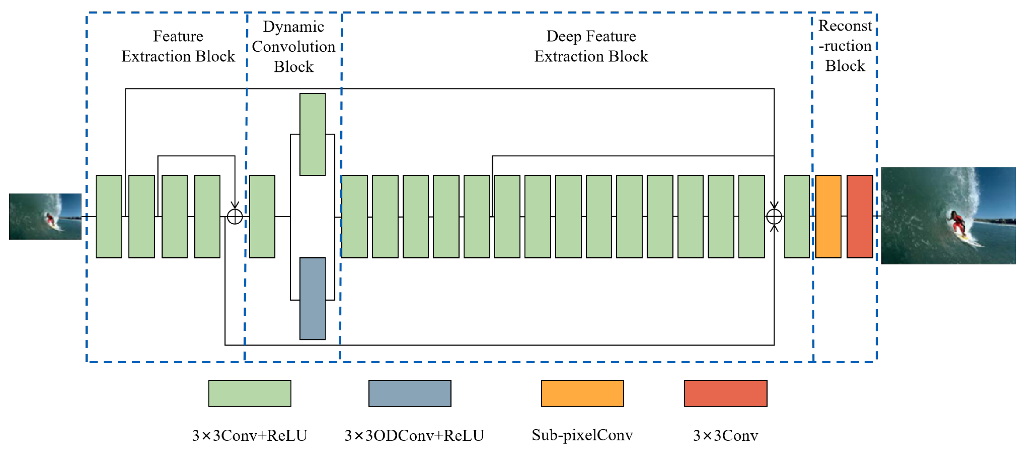
Figure 1 illustrates the overall architecture of ODConvNet, consisting of four sequential modules: a Feature Extraction Block (FEB), a Dynamic Convolution Block (DCB), a Deep Feature Extraction Block (DFEB), and a Reconstruction Block (RB). Each block is designed with specific responsibilities: FEB captures low-level spatial features; DCB introduces adaptive feature modulation via dynamic convolution; DFEB performs progressive deep feature refinement; and RB reconstructs the final high-resolution output. The arrows between modules indicate data flow, and internal skip connections are shown where applicable.

Specifically, the input LR image is first processed by the FEB, which employs four sequential convolutional layers combined with ReLU activation functions. Residual connections are introduced within the FEB to preserve shallow features and improve the model’s capability to memorize and represent detailed image structures. Then, these low-frequency features are input to the DCB block for further enhancement and refinement of the features. To enhance feature flexibility and adaptability, the DCB integrates Omni-dimensional Dynamic Convolution (ODConv) and traditional convolution operations in parallel. This allows the network to dynamically adjust convolution kernels based on input features across kernel-wise, spatial, input channel, and output channel dimensions, enhancing feature robustness. The outputs from these convolution operations are weighted and merged through a learnable scalar $\alpha$, providing an effective trade-off between dynamic adaptability and computational efficiency. Following the DCB, the DFEB, comprising 15 convolutional layers with ReLU activations, is designed to further extract and refine deeper feature representations. By stacking multiple convolutional layers, DFEB significantly enhances the depth and expressiveness of features, capturing complex image structures and subtle texture details.To reconstruct high-quality SR images, the RB utilizes a two-stage upsampling strategy. Initially, a subpixel convolution layer is employed to upscale low-frequency features into high-frequency representations, effectively enlarging image dimensions. Subsequently, a $3\times 3$ convolutional layer refines high-frequency information, precisely reconstructing and synthesizing image details. In summary, the SR process using ODConvNet can be described as

$$I_H=ODConvNet\left(I_L\right)=RB\left(DFEB\left(DCB\left(FEB\left(I_L\right)\right)\right)\right)$$

(1)

where $I_{\mathrm{L}}$ is the input low-resolution image, $\mathit{ODConvNet}$ denotes the network, and $\mathit{FEB}$, $\mathit{DCB}$, $\mathit{DFEB}$, and $\mathit{RB}$ represent the function of FEB, DCB, DFEB, and RB, respectively.

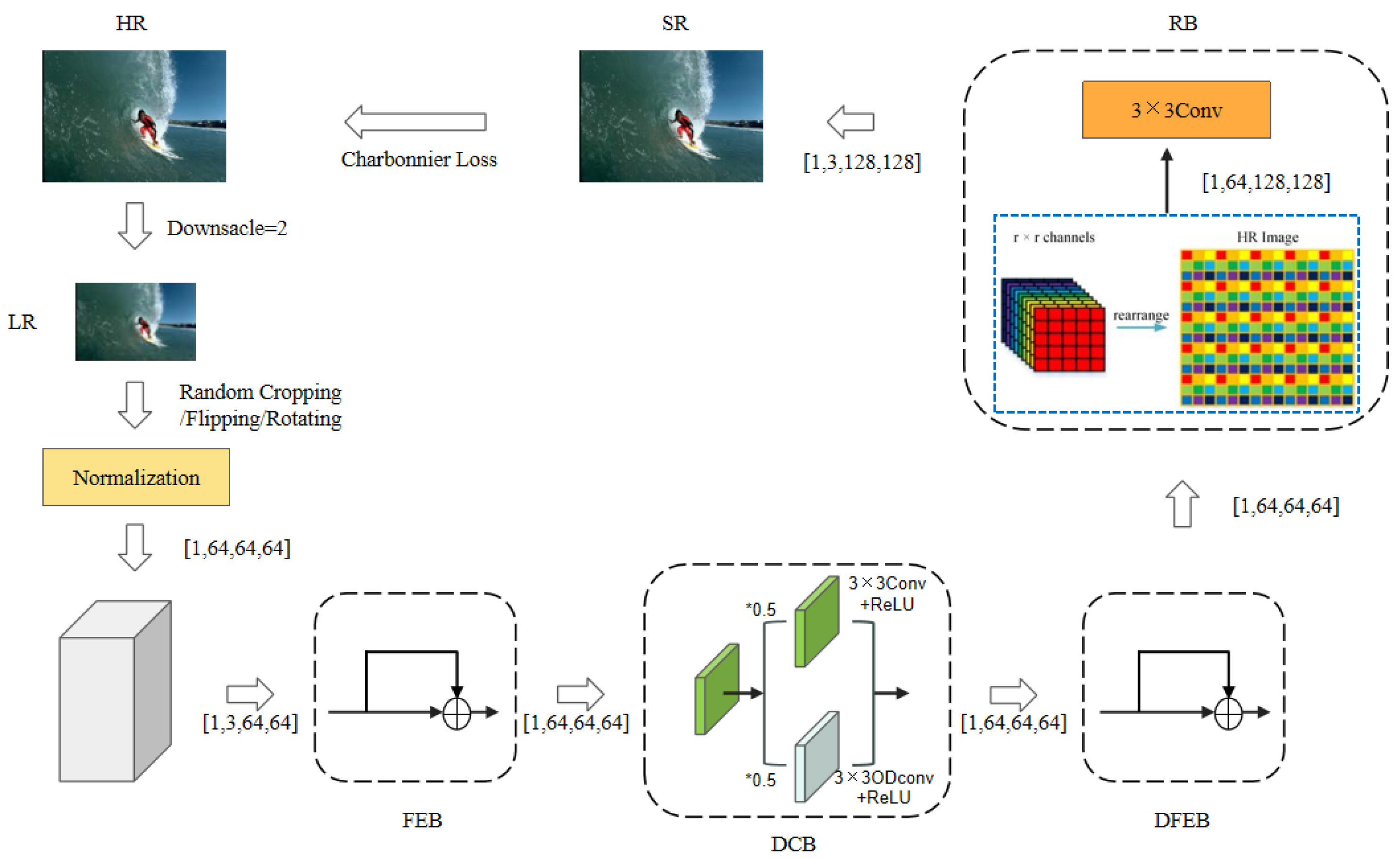
The complete data flow and processing pipeline of ODConvNet are illustrated in Figure 2. The input low-resolution (LR) image undergoes random data augmentation and normalization before being fed into the network. The FEB captures shallow features, which are enhanced via both standard and dynamic convolutions in the DCB. These features are further refined through deep residual layers in the DFEB, followed by subpixel convolution and refinement in the RB to produce the final high-resolution (HR) image. Charbonnier loss is applied between the SR output and the ground truth HR image during training.

3.2. Feature Extraction Block

The Feature Extraction Block (FEB) serves as the initial component of ODConvNet, designed specifically to extract and enhance low-level features from the input low-resolution image. FEB is comprised of four sequential convolutional layers, each paired with a ReLU activation function to introduce nonlinearity and facilitate effective feature learning. Each convolutional layer uses a 3 × 3 kernel, where the first layer processes the 3-channel RGB input, and the subsequent layers maintain 64 output channels.

To effectively capture essential structural details such as edges and textures, the FEB employs residual learning, enabling better retention and propagation of shallow features throughout the network. Specifically, residual connections are strategically implemented between convolutional layers, combining outputs from earlier and subsequent layers to preserve valuable information and enhance the expressive capability of shallow representations.

The computational procedure of the FEB can be formally described as follows:

$$F_{FEB}=4ReLU\left(Conv\left(I_L\right)\right)+2ReLU\left(Conv\left(I_L\right)\right)$$

(2)

where $I_L$ denotes the input LR image, and $\mathit{nReLU}\left(\mathit{Conv}\right(\left)\right)$ represents n consecutive convolutional and ReLU layers.

The FEB thus plays a pivotal role in preparing a robust and discriminative feature foundation, enabling deeper subsequent blocks of ODConvNet to further refine and reconstruct high-quality, high-resolution images.

3.3. Dynamic Convolution Block

The proposed model defines the dynamics of the network as the process of adaptively modulating convolution kernel weights according to the input feature map through attention applied along four axes: kernel index, spatial position, input channel, and output channel. This is implemented via the use of an Omni-dimensional Dynamic Convolution (ODConv) layer. To fully leverage this capability, we design the Dynamic Convolution Block (DCB) by integrating the ODConv module with a standard convolution branch in a parallel structure. The outputs of both branches are fused through a learnable scalar weight, enabling the model to balance adaptability and stability. This architectural design enhances ODConvNet’s flexibility and feature representation, allowing it to dynamically adjust convolution behavior across multiple dimensions and effectively capture diverse features, particularly in scenarios with complex spatial or structural variations.

Specifically, the DCB employs two parallel convolutional branches. One branch applies an ODConv layer, which adaptively adjusts convolutional kernel weights through learned attention mechanisms in kernel-wise, spatial, input-channel, and output-channel dimensions. The other branch employs a traditional convolutional layer to maintain stable feature extraction capabilities. The outputs from these two branches are then combined through a learnable scalar parameter $\alpha$, enabling the network to dynamically balance feature contributions from each branch. The architecture of the ODConv layer is illustrated in Figure 3, which shows the detailed components and flow of the ODConv operation.

Formally, the operation of DCB can be expressed as follows:

$$F_{DCB}=\alpha ·ODConv\left(F_{\mathrm{FEB}}\right)+(1-\alpha )·Conv\left(F_{\mathrm{FEB}}\right)$$

(3)

where $F_{FEB}$ represents the shallow features output from the FEB module, $ODConv(·)$ denotes the Omni-dimensional Dynamic Convolution operation, and $Conv(·)$ denotes a conventional convolution operation. The scalar parameter $\alpha$ is learnable during training and determines the relative weight assigned to dynamic and conventional convolutions.

Specifically, given an input feature map X, the output of the ODConv operation is formulated as

$$Y=\sum _{k=1}^K{\mathcal{A}}_k·\left({\mathcal{A}}_{\mathrm{out}}\otimes \left({\mathcal{A}}_{\mathrm{in}}\otimes \left({\mathcal{A}}_{\mathrm{spatial}}\otimes (W_k\ast X)\right)\right)\right)$$

(4)

where $W_k$ denotes the k-th convolution kernel, ∗ represents the convolution operation, and ⊗ indicates element-wise multiplication. ${\mathcal{A}}_k$, ${\mathcal{A}}_{\mathrm{out}}$, ${\mathcal{A}}_{\mathrm{in}}$, and ${\mathcal{A}}_{\mathrm{spatial}}$ correspond to the kernel-wise, output-channel-wise, input-channel-wise, and spatial-wise attention weights, respectively.

The generation of attention weights begins with a global average pooling (GAP) applied to X across spatial dimensions, producing a channel-wise descriptor $z\in {\mathbb{R}}^C$:

$$z_c={\displaystyle \frac{1}{H\times W}}\sum _{i=1}^H\sum _{j=1}^W{X}_c(i,j)$$

(5)

This descriptor is then mapped to a low-dimensional embedding through a fully connected (FC) layer:

$$z^{\prime }=FC\left(z\right)$$

(6)

Finally, the four attention maps are generated by applying the sigmoid activation function to the transformed features:

$${\mathcal{A}}_k,{\mathcal{A}}_{\mathrm{out}},{\mathcal{A}}_{\mathrm{in}},{\mathcal{A}}_{\mathrm{spatial}}=\sigma \left(z^{\prime }\right)$$

(7)

where $\sigma (·)$ denotes the element-wise sigmoid function.

Through this mechanism, ODConv dynamically adapts its kernels to better suit the input content, offering greater flexibility in handling diverse structural variations within images. The inclusion of ODConv enhances the network’s capability to extract meaningful features and improves its robustness in high-frequency detail recovery, thereby delivering superior performance in SR tasks.

3.4. Deep Feature Extraction Block

The Deep Feature Extraction Block (DFEB) is specifically designed to further refine and enrich feature representations extracted from the preceding Dynamic Convolution Block (DCB). By stacking multiple convolutional layers, the DFEB enhances the depth and complexity of the extracted features, thereby capturing detailed textures and semantic structures necessary for effective SR reconstruction.

In particular, DFEB comprises a sequential stack of 15 convolutional layers, each paired with a ReLU activation function to ensure nonlinear transformations and stable gradient flow. This stacked architecture allows the network to progressively distill complex image information from shallower to deeper layers, enabling the effective capture of both fine-grained local details and broader contextual semantics.

The operation of the DFEB can be formally described as follows:

$$\begin{array}{cc}\hfill F_{DFEB}=& ReLU\left(Conv\right(14ReLU\left(Conv\left(I_{DCB}\right)\right)+5ReLU\left(Conv\left(I_{DCB}\right)\right)\hfill \\ \hfill & +ReLU\left(Conv\left(I_L\right)\right)+4ReLU\left(Conv\left(I_L\right)\right)\left)\right)\hfill \end{array}$$

(8)

where $F_{DCB}$ represents the features obtained from the Dynamic Convolution Block, $F_{DFEB}$ denotes the resulting deeply extracted feature representation, $I_L$ is the input LR image, and $nReLU\left(Conv\right(\left)\right)$ represents n consecutive convolutional and ReLU layers.

By aggregating these deep, hierarchical feature representations, DFEB significantly improves the network’s ability to recover intricate image structures and subtle high-frequency details, ultimately contributing to superior image reconstruction quality in single-image SR tasks.

3.5. Restruction Block

The RB is the final component in the ODConvNet architecture, specifically designed to transform the deeply extracted features into a HR image. The RB employs a two-stage upsampling strategy to accurately reconstruct and refine detailed high-frequency textures, effectively improving the visual fidelity of the final output.

Initially, a subpixel convolution layer is utilized to upscale the spatial dimensions of the deep feature maps, effectively converting learned low-frequency information into refined high-frequency details. Subsequently, a convolutional refinement layer follows to precisely enhance the reconstructed image, refining edges and textures for improved visual quality.

Formally, the reconstruction process can be described as

$$I_H=Conv\left(SubPixelConv\left(F_{DFEB}\right)\right)$$

(9)

where $F_{DFEB}$ represents the deep features obtained from the Deep Feature Extraction Block, $SubPixelConv(·)$ denotes the subpixel convolution operation for spatial upscaling, and $Conv(·)$ represents the final convolutional refinement layer. $I_H$ is the final output, representing the reconstructed HR image.

By integrating these modules, the Reconstruction Block effectively synthesizes the hierarchical features extracted by previous layers, accurately reconstructing high-frequency textures and ensuring high-quality SR results.

3.6. Loss Function

The loss function is a non-negative real-valued function that quantifies the discrepancy between the predicted output $f\left(x\right)$ of the model and the ground truth label Y. It is denoted as $\mathcal{L}\left(f\right(x),Y)$, and a smaller loss value typically indicates better robustness and accuracy of the model. During training, a batch of input data is passed through the network to obtain predictions via forward propagation. The loss function then evaluates the prediction error, and its value is used to guide backpropagation, allowing the model to update its parameters and reduce the difference between predicted and actual values iteratively.

In conventional SISR tasks, the L1 loss [44] and L2 loss [45] are widely used. The L1 loss computes the mean absolute error between predictions and ground truth, offering robustness to outliers, but it suffers from discontinuous gradients, resulting in slower convergence. In contrast, the L2 loss minimizes the squared error, providing smoother gradient updates and faster convergence, yet it is sensitive to outliers and may cause gradient explosion.

To overcome these limitations, we adopted the Charbonnier loss [46] as the optimization objective in our network. Charbonnier loss is a differentiable variant of the L1 loss that is robust to noise while maintaining stable gradient computation. As illustrated in Equation (10), it introduces a small constant $ϵ$ to ensure differentiability at zero and smooth convergence:

$${\mathcal{L}}_{\mathrm{Char}}(x,y)={\displaystyle \frac{1}{N}}\sum _{i=1}^N\sqrt{{(x_i-y_i)}^2+{ϵ}^2}$$

(10)

where $x_i$ denotes the predicted pixel value, $y_i$ represents the corresponding ground truth, N is the total number of pixels, and $ϵ$ is a small constant (typically set to ${10}^{-3}$) to guarantee numerical stability and differentiability at $x=y$. The Charbonnier loss approximates the L1 norm near zero and ensures smooth gradient flow across the entire input domain.

By combining the advantages of both L1 and L2 losses, the Charbonnier loss achieved a balanced trade-off between convergence speed and robustness to outliers. This makes it particularly suitable for SR tasks, where subtle detail preservation and noise resilience are both essential. In our experiments, the adoption of Charbonnier loss contributed significantly to stable training and high-quality image reconstruction.

4. Experiment

4.1. Conducted Datasets

To comprehensively evaluate the effectiveness and robustness of the proposed ODConvNet, extensive experiments were conducted using publicly available benchmark datasets commonly employed for SISR tasks. Specifically, we selected the widely recognized DIV2K [47] dataset for model training and validation and four additional standard datasets, namely, Set5 [48], Set14 [49], B100 [50], and Urban100 [51], for comprehensive performance evaluation.

The DIV2K dataset contains 800 high-resolution images for training and 100 images for validation. During the training phase, the 800-image training set was employed, while the validation set was used to monitor the convergence and select optimal model checkpoints. The four benchmark datasets are widely adopted to rigorously test SR algorithms across diverse scenarios: Set5 [48] consists of five natural images commonly utilized as a baseline for initial performance evaluation. Set14 [49] includes 14 images representing a variety of textures and structures, providing a balanced evaluation of reconstruction capability. B100 [50] contains 100 diverse images from the Berkeley segmentation dataset extensively used to evaluate reconstruction consistency and robustness. Urban100 [51] comprises 100 urban scenes featuring complex architectural structures extensively utilized to test the model’s ability to recover detailed textures and geometrical patterns.

All images were converted into the YCbCr color space, and quantitative evaluations were performed exclusively on the luminance (Y) channel, following common practice in the literature. The Peak Signal-to-Noise Ratio (PSNR) and Structural Similarity Index (SSIM) were used as primary metrics to quantitatively assess SR quality and effectiveness. Additionally, we adopted the Feature Similarity Index (FSIM) and Learned Perceptual Image Patch Similarity (LPIPS) as supplementary perceptual metrics, where the FSIM evaluates structural fidelity based on phase congruency and gradient information, and LPIPS leverages deep neural network features to align with human visual perception.

PSNR quantifies image quality by calculating the mean squared error between the original and reconstructed images. As illustrated in Equation (11), the mathematical formulation is

$$PSNR=10·{log}_{10}\left({\displaystyle \frac{MA{X}_I^2}{MSE}}\right)$$

(11)

where $MA{X}_I$ represents the maximum possible pixel value, and $MSE$ denotes the mean squared error between the two images. The PSNR is measured in decibels (dB), with higher values indicating smaller differences between the reconstructed and original images and thus better quality.

The SSIM evaluates image similarity from three dimensions of human visual perception: luminance, contrast, and structure. It follows the formulation in Equation (12):

$$SSIM(x,y)={\displaystyle \frac{(2{\mu }_x{\mu }_y+C_1)(2{\sigma }_{xy}+C_2)}{({\mu }_x^2+{\mu }_y^2+C_1)({\sigma }_x^2+{\sigma }_y^2+C_2)}}$$

(12)

where $\mu$ represents the local mean, $\sigma$ denotes the standard deviation, ${\sigma }_{xy}$ is the covariance, and $C_1$ and $C_2$ are stabilization constants. The SSIM output ranges from 0 to 1, with values closer to 1 indicating higher structural similarity between images and better perceptual quality.

The FSIM evaluates the perceptual similarity between images by incorporating low-level features that closely align with the Human Visual System (HVS), primarily the Phase Congruency (PC) and Gradient Magnitude (GM). It is designed to capture salient structural information and visual attention. The mathematical formulation of FSIM is expressed in Equation (13):

$$FSIM={\displaystyle \frac{{\sum }_{x\in \Omega }T\left(x\right)·P{C}_m\left(x\right)}{{\sum }_{x\in \Omega }P{C}_m\left(x\right)}}$$

(13)

where $\Omega$ denotes the spatial domain of the image, $P{C}_m\left(x\right)$ is the maximum phase congruency at location x, and $T\left(x\right)$ is the similarity function combining phase congruency and gradient magnitude similarities at pixel x. The FSIM values range from 0 to 1, with higher values indicating better perceptual quality and structural fidelity.

The LPIPS is a deep learning-based perceptual metric that measures the distance between image patches using features extracted from pretrained convolutional neural networks. It aligns well with human perceptual judgments. The LPIPS distance is defined in Equation (14):

$$LPIPS(x,y)=\sum _l{\displaystyle \frac{1}{H_l{W}_l}}\sum _{h,w}{\left|w_l\odot \left({\widehat{f}}_l^x(h,w)-{\widehat{f}}_l^y(h,w)\right)\right|}_2^2$$

(14)

where $f_l^x$ and $f_l^y$ are the deep features extracted at layer l for images x and y, respectively, $\widehat{f}$ denotes channel-wise unit normalization, $w_l$ are learned weights for each channel, and $(H_l,W_l)$ are the spatial dimensions of layer l. Lower LPIPS values indicate better perceptual similarity.

4.2. Experimental Setting

The experimental environment setup was the following: The operating system was Ubuntu 20.04.5, and the hardware configuration included an AMD EPYC 7502P 32-Core Processor (Advanced Micro Devices, Inc., Santa Clara, CA, USA), a RTX 3090 GPU (NVIDIA Corporation, Santa Clara, CA, USA), and 128 GB of RAM. The model code used in the experiments was written in Python, version 3.8.18. Additionally, the version of CUDA used was 11.7.

For experimental setups, we followed standard practice in SISR research by feeding low-resolution RGB images into the network. This ensured consistency with the preprocessing pipelines of prior work and enabled fair comparisons across benchmarks.

The overall architecture consists of four consecutive components: the Feature Extraction Block (FEB), the Dynamic Convolution Block (DCB), the Deep Feature Extraction Block (DFEB), and the Reconstruction Block (RB). Specifically, the FEB comprises four 3 × 3 convolutional layers, with each followed by a ReLU activation. The DCB integrates a 3 × 3 convolutional layer in a parallel structure that combines both dynamic convolution and standard convolution. The DFEB stacks fifteen 3 × 3 convolutional layers with ReLU activations to progressively refine features. Finally, the RB employs a subpixel convolution layer followed by a 3 × 3 convolutional layer to reconstruct the high-resolution output, producing a 3-channel RGB image.

For the hyperparameter setup, the batch size was set to 64, and the image patch size was 64. Data augmentation strategies included random cropping, random flipping, and random rotation, followed by normalization. The Adam [52] optimizer was used, with an initial learning rate of 0.0001, which was halved every 400,000 iterations. The PSNR and SSIM were used to evaluate the SR performance.

In the experimental configuration, each epoch consisted of 1000 iterations, and the model was trained for a total of 900 epochs. For ablation studies, 600 epochs were run, with the batch size and image patch size adjusted to 32 and 16, respectively.

4.3. Experimental Analysis

The proposed ODConvNet integrates three essential components: the Charbonnier loss function, the ODConv module, and a residual network structure. These are specifically designed to enhance feature representation, improve robustness to outliers, and facilitate gradient flow, ultimately contributing to superior performance in the SISR task. Therefore, this section presents a detailed analysis of each component and their combined effect through a series of ablation experiments on the Set5, Set14, and B100 datasets, with a 4× upscaling factor.

The Charbonnier loss replaces the traditional L2 loss function in the baseline model. Unlike L2 loss, which is sensitive to outliers, Charbonnier loss is a differentiable approximation of the L1 norm, providing better convergence and stability during training. As shown in

Table 1. Ablation study of ODConvNet on B100 for ×4 super-resolution.

Methods	Set5 (PSNR/SSIM)	Set14 (PSNR/SSIM)	B100 (PSNR/SSIM)
Baseline	31.52/0.8854	27.96/0.7737	27.37/0.7284
+ Charbonnier Loss	31.62/0.8877	27.99/0.7757	27.41/0.7305
+ ODConv	31.75/0.8890	28.05/0.7764	27.42/0.7312
+ Residual Structure	31.79/0.8894	28.07/0.7764	27.44/0.7312

, introducing the Charbonnier loss improved the PSNR on Set5 from 31.52 dB to 31.62 dB and the SSIM from 0.8854 to 0.8877, demonstrating its superior error modeling capability and robustness.

ODConv module: The ODConv module is designed to dynamically adjust convolutional kernels across multiple dimensions, including spatial, channel, and kernel axes. When integrated with the Charbonnier loss, the model achieved significant performance gains, with the PSNR increasing to 31.75 dB and SSIM to 0.8890 on Set5. These results suggest that ODConv enhances the network’s ability to capture spatially adaptive features and complex image structures.

Residual network structure: To further improve information flow and feature reuse, we incorporated a residual network design atop the Charbonnier loss and ODConv-based backbone. This structure facilitates deeper networks without degradation, enabling finer reconstruction of high-frequency details. The full model, with all three components, achieved the best performance—31.79 dB PSNR and 0.8894 SSIM on Set5—along with consistent improvements on Set14 and B100.

These results collectively validate the individual effectiveness of each component, and more importantly, their synergistic contribution to the overall performance of ODConvNet in SISR tasks. Additionally, ODConvNet demonstrates competitive computational efficiency, with training times and memory usage comparable to other advanced models like VDSR and DnCNN. Despite the increased complexity due to dynamic convolutions, ODConvNet maintains practical computational requirements, making it suitable for real-time applications. Qualitative results also highlight the superior visual quality of ODConvNet, particularly on challenging datasets like U100, where the network preserves fine details such as textures and edges more effectively than other methods. At higher scaling factors ($\times 3$ and $\times 4$), ODConvNet shows a notable reduction in artifacts such as blurring and aliasing, ensuring a clearer and more accurate reconstruction. Overall, the experimental results confirm that ODConvNet is a powerful and efficient solution for SISR, offering both high-quality image reconstruction and practical applicability for real-world tasks.

4.4. Experimental Results

This section presents the quantitative evaluation of ODConvNet across standard benchmark datasets (Set5, B100, and U100) at three magnification scales ($\times 2$, $\times 3$, and $\times 4$). Comparative analysis with contemporary advanced methods was conducted using the established image quality metrics PSNR and SSIM.

The results show that ODConvNet outperformed all the compared methods across all datasets and scaling factors. As shown in

Table 2. Performance comparison on Set5 at (×2, ×3, ×4) magnifications, evaluated using PSNR (dB) and SSIM metrics. Red and blue represent the best and second-best results, respectively.

Datasets	Methods	×2	×3	×4
Set5	Bicubic [27]	33.66/0.9299	30.39/0.8682	28.42/0.8104
	SRCNN [14]	36.66/0.9542	32.75/0.9090	30.48/0.8628
	A+ [32]	36.54/0.9544	32.58/0.9088	30.28/0.8603
	ScSR [53]	35.78/0.9485	31.34/0.8869	29.07/0.8263
	JOR [54]	36.58/0.9543	32.55/0.9067	30.19/0.8563
	FSRCNN [18]	37.00/0.9558	33.16/0.9140	30.71/0.8657
	RFL [55]	36.54/0.9537	32.43/0.9057	30.14/0.8548
	SelfEx [51]	36.49/0.9537	32.58/0.9093	30.31/0.8619
	CSCN [56]	36.93/0.9552	33.10/0.9144	30.86/0.8732
	VDSR [15]	37.53/0.9587	33.66/0.9213	31.35/0.8838
	RED [16]	37.56/0.9595	33.70/0.9222	31.33/0.8847
	DnCNN [57]	37.58/0.9590	33.75/0.9222	31.40/0.8845
	TNRD [58]	36.86/0.9556	33.18/0.9152	30.85/0.8732
	RCN [59]	37.17/0.9583	33.45/0.9175	31.11/0.8736
	DRCN [60]	37.63/0.9588	33.82/0.9226	31.53/0.8854
	CNF [61]	37.66/0.9590	33.74/0.9226	31.55/0.8856
	LapSRN [17]	37.52/0.9590	-	31.54/0.8850
	WaveResNet [62]	37.57/0.9586	33.86/0.9228	31.52/0.8864
	CPCA [63]	34.99/0.9469	31.09/0.8975	28.67/0.8434
	FDSR [64]	37.40/0.9513	33.68/0.9096	31.28/0.8658
	LESRCNN [65]	37.65/0.9586	33.93/0.9231	31.88/0.8903
	IDENet [66]	37.16/0.9521	-	31.57/0.8846
	GLFDN [67]	37.47/0.9545	33.86/0.9203	31.90/0.8869
	DSRNet [24]	37.61/0.9584	33.92/0.9227	31.71/0.8874
	ODConvNet (Ours)	37.72/0.9593	34.06/0.9243	31.90/0.8914

, on the Set5 dataset, ODConvNet achieved a PSNR of 37.72 dB and an SSIM of 0.9593 at $\times 2$, which was superior to other methods such as Bicubic, SRCNN, and VDSR. Similarly, as shown in

Table 3. Performance comparison on B100 at (×2, ×3, ×4) magnifications, evaluated using PSNR (dB) and SSIM metrics. Red and blue represent the best and second-best results, respectively.

Datasets	Methods	×2	×3	×4
B100	Bicubic [27]	29.56/0.8431	27.21/0.7385	25.96/0.6675
	A+ [32]	31.21/0.8863	28.29/0.7835	26.82/0.7087
	SRCNN [14]	31.36/0.8879	28.41/0.7863	26.90/0.7101
	JOR [54]	31.22/0.8867	28.27/0.7837	26.79/0.7083
	RFL [55]	31.16/0.8840	28.22/0.7806	26.75/0.7054
	SelfEx [51]	31.18/0.8855	28.29/0.7840	26.84/0.7106
	CSCN [56]	31.40/0.8884	28.50/0.7885	27.03/0.7161
	FSRCNN [18]	31.53/0.8920	28.53/0.7910	26.98/0.7150
	RED [16]	31.96/0.8972	28.88/0.7993	27.35/0.7276
	TNRD [58]	31.40/0.8878	28.50/0.7881	27.00/0.7140
	VDSR [15]	31.90/0.8960	28.82/0.7976	27.29/0.7251
	DRCN [60]	31.85/0.8942	28.80/0.7963	27.23/0.7233
	DRRN [68]	32.05/0.8973	28.95/0.8004	27.38/0.7284
	CNF [61]	31.91/0.8962	28.82/0.7980	27.32/0.7253
	LapSRN [17]	31.80/0.8950	-	27.32/0.7280
	ScSR [53]	30.77/0.8744	27.72/0.7647	26.61/0.6983
	DnCNN [57]	31.90/0.8961	28.85/0.7981	27.29/0.7253
	CARN-M [47]	31.92/0.8960	28.91/0.8000	27.44/0.7304
	FDSR [64]	31.87/0.8847	28.82/0.7797	27.31/0.7031
	NDRCN [69]	32.00/0.8975	28.86/0.7991	27.30/0.7263
	LESRCNN [65]	31.95/0.8964	28.91/0.8005	27.45/0.7313
	IDENet [66]	31.65/0.8848	-	27.35/0.7235
	DSRNet [24]	31.96/0.8965	28.90/0.8003	27.43/0.7303
	ODConvNet (Ours)	32.06/0.8981	28.97/0.8017	27.48/0.7332

, ODConvNet achieved a PSNR of 32.06 dB and an SSIM of 0.8981 at $\times 2$ on B100, surpassing methods like LESRCNN and NDRCN. In more complex urban landscapes in U100, ODConvNet was also able to achieve optimal performance. As shown in

Table 4. Performance comparison on U100 at (×2, ×3, ×4) magnifications, evaluated using PSNR (dB) and SSIM metrics. Red and blue represent the best and second-best results, respectively.

Datasets	Methods	×2	×3	×4
U100	Bicubic [27]	26.88/0.8403	24.46/0.7349	23.14/0.6577
	A+ [32]	29.20/0.8938	26.03/0.7973	24.32/0.7183
	SRCNN [14]	29.50/0.8946	26.24/0.7989	24.52/0.7221
	JOR [54]	29.25/0.8951	25.97/0.7972	24.29/0.7181
	RFL [55]	29.11/0.8904	25.86/0.7900	24.19/0.7096
	SelfEx [51]	29.54/0.8967	26.44/0.8088	24.79/0.7374
	FSRCNN [18]	29.88/0.9020	26.43/0.8080	24.62/0.7280
	RED [16]	30.91/0.9159	27.31/0.8303	25.35/0.7587
	TNRD [58]	29.70/0.8994	26.42/0.8076	24.61/0.7291
	VDSR [15]	30.76/0.9140	27.14/0.8279	25.18/0.7524
	DRCN [60]	30.75/0.9133	27.15/0.8276	25.14/0.7510
	DRRN [68]	31.23/0.9188	27.53/0.8378	25.44/0.7638
	LapSRN [17]	30.41/0.9100	-	25.21/0.7560
	WaveResNet [62]	30.96/0.9169	27.28/0.8334	25.36/0.7614
	ScSR [53]	28.26/0.8828	-	24.02/0.7024
	IDN [70]	31.27 /0.9196	27.42/0.8359	25.41/0.7632
	FDSR [64]	30.91/0.9088	27.23/0.8190	25.27/0.7417
	NDRCN [69]	31.06/0.9175	27.23/0.8312	25.16/0.7546
	DnCNN [57]	30.74/0.9139	27.15/0.8276	25.20/0.7521
	CARN-M [47]	31.23/0.9193	27.55/0.8385	25.62/0.7694
	MemNet [71]	31.31/0.9195	27.56/0.8376	25.50/0.7630
	IDENet [66]	30.22/0.9004	-	25.39/0.7585
	DSRNet [24]	31.41/0.9209	27.63/0.8402	25.65/0.7693
	ODConvNet (Ours)	31.81/0.9253	27.77/0.8441	25.75/0.7761

, ODConvNet achieved the highest PSNR of 31.81 dB and SSIM of 0.9253, outperforming all other competing methods. To provide a more comprehensive evaluation beyond traditional distortion-based metrics, we supplemented the PSNR and SSIM with perceptual metrics such as the FSIM and LPIPS. These indicators better reflect human visual perception and help assess the realism of reconstructed textures. As shown in

Table 5. Performance metrics of different models on the Urban100 dataset for the ×4 super-resolution images.

Methods	PSNR (dB)	SSIM	FSIM	LPIPS
Bicubic [27]	23.14	0.6577	0.9415	0.4727
SRCNN [14]	24.52	0.7221	0.9671	0.3516
SelfEx [51]	24.79	0.7374	0.9761	0.3098
CARN-M [47]	25.62	0.7694	0.9811	0.2524
ODConvNet (Ours)	25.76	0.7767	0.9816	0.2372

, our ODConvNet achieved the best performance across all four metrics on the Urban100 dataset.

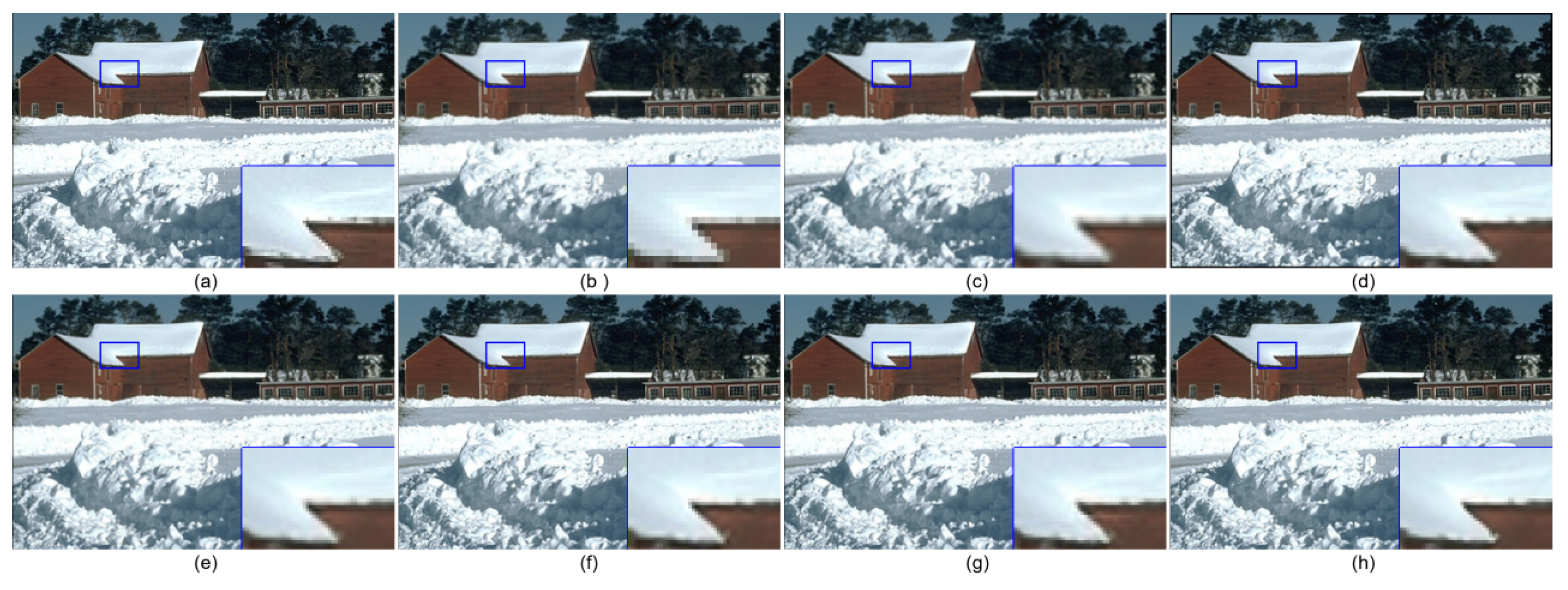
In addition to the quantitative performance, the qualitative results also demonstrate the superiority of ODConvNet. Visual inspection of the super-resolution images reveals that ODConvNet was able to recover finer details, such as textures and edges, more effectively than other methods. As shown in Figure 4, we conducted a comparative analysis on img100 in the B100 test set. By comparison, we can observe that the SR technology proposed in this section is significantly better than other methods in terms of authenticity. For example, in the enlarged area in the Figure 4, other traditional interpolation methods and deep learning methods failed to effectively restore the second corner of the snow edge in the original image, while the method proposed in this section successfully reconstructed the details of the snow edge, which is more in line with the visual perception of the human eye. 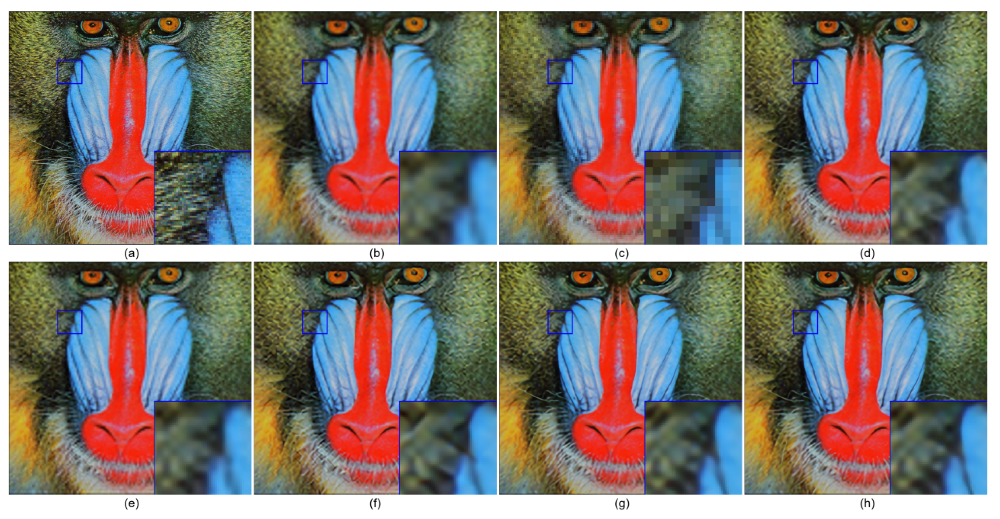In addition, through comparative analysis of the img011 image in the Set14 test set in the Figure 5, it can be clearly seen that ODConvNet restored the edge part of the butterfly wing texture more realistically and closer to the area shown in the original image, showing superiority compared to the contrasting interpolation method and deep learning method. Finally, we selected the img011 image in the Set14 test set for comparative analysis. It can be clearly observed that the ODConvNet method achieved better clarity in visual presentation. In particular, in the enlarged area shown in the Figure 6, this method is more realistic in restoring the color boundary of the mandrill’s face, with more accurate colors and closer to the area shown in the original image, showing its obvious superiority compared to other interpolation methods and deep learning methods.

As shown in

Table 6. Complexity of different super-resolution methods at a scaling factor of 4 and image size of 256 × 256. The performance was evaluated on the B100 dataset with scaling factors of ×2, ×3, and ×4.

Methods	Parameters (M)	FLOPs (G)	PSNR/SSIM (B100 ×2)	PSNR/SSIM (B100 ×3)	PSNR/SSIM (B100 ×4)
LESRCNN [65]	0.6263	70.5	31.95/0.8964	28.91/0.8005	27.45/0.7313
CARN-M [47]	0.5335	35.4	31.92/0.8960	28.91/0.8000	27.44/0.7304
EMASRN [72]	0.5332	480.3	-	29.05/0.8035	27.55/0.7351
ODConvNet (Ours)	0.9651	98.73	32.06/0.8981	28.97/0.8017	27.48/0.7332

, our proposed ODConvNet achieved the best overall performance across all scaling factors on the B100 dataset while maintaining a favorable trade-off between model complexity and computational cost. Specifically, ODConvNet obtained the highest PSNR/SSIM at ×2 (32.06/0.8981), ×3 (28.97/0.8017), and ×4 (27.48/0.7332), outperforming the advanced methods such as LESRCNN, CARN-M, and EMASRN. Although ODConvNet has a moderately higher parameter count (1.8692 M) than CARN-M and LESRCNN, it avoids the excessive FLOPs of EMASRN (480.3 G), operating efficiently at 98.58 GFLOPs. These results demonstrate that ODConvNet not only delivers superior reconstruction quality but also maintains computational efficiency, making it well suited for both high-performance and resource-constrained SR applications.

The experimental results demonstrate ODConvNet’s advanced performance across all metrics, surpassing existing methods in PSNR/SSIM scores, visual quality, and computational efficiency and making it particularly suitable for practical deployment.

5. Conclusions

In this paper, we present ODConvNet, a novel SISR architecture integrating dynamic convolutions with hierarchical feature extraction. The network achieved advanced performance across Set5, Set14, B100, and U100 benchmarks, excelling in both objective metrics (PSNR/SSIM) and subjective quality while maintaining computational efficiency for practical applications.

The ablation studies further reveal the importance of the Dynamic Convolution Block (DCB) and the Deep Feature Extraction Block (DFEB) in enhancing the network’s ability to recover fine-grained image details and adapt to dynamic feature scales. These components contribute significantly to ODConvNet’s ability to achieve superior results across a range of image complexities and scaling factors.

Additionally, ODConvNet maintains competitive training times and memory usage, even with the increased complexity due to dynamic convolutions. This makes the network an efficient solution for high-quality image reconstruction in real-time applications.

Overall, ODConvNet represents a promising approach for SISR, offering both high-quality results and practical applicability for a wide range of imaging tasks. Its codes can be available at https://github.com/chenxi12434/ODConvNet (accessed on 22 July 2025).

References

1. Park, S.C.; Park, M.K.; Kang, M.G. Super-resolution image reconstruction: A technical overview. IEEE Signal Process. Mag. 2003, 20, 21–36. [Google Scholar] [CrossRef]
2. Tian, C.; Zheng, M.; Li, B.; Zhang, Y.; Zhang, S.; Zhang, D. Perceptive self-supervised learning network for noisy image watermark removal. IEEE Trans. Circuits Syst. Video Technol. 2024, 34, 7069–7079. [Google Scholar] [CrossRef]
3. Peng, C.; Zhou, S.K.; Chellappa, R. DA-VSR: Domain adaptable volumetric super-resolution for medical images. In Proceedings of the International Conference on Medical Image Computing and Computer-Assisted Intervention, Strasbourg, France, 27 September–1 October 2021; Springer: Cham, Switzerland, 2021; pp. 75–85. [Google Scholar]
4. Lu, T.; Wang, J.; Zhang, Y.; Wang, Z.; Jiang, J. Satellite image super-resolution via multi-scale residual deep neural network. Remote Sens. 2019, 11, 1588. [Google Scholar] [CrossRef]
5. Aakerberg, A.; Nasrollahi, K.; Moeslund, T.B. Real-world super-resolution of face-images from surveillance cameras. IET Image Process. 2022, 16, 442–452. [Google Scholar] [CrossRef]
6. Ma, L.; Zhou, Y.; Ma, Y.; Yu, G.; Li, Q.; He, Q.; Pei, Y. Defying Multi-model Forgetting in One-shot Neural Architecture Search Using Orthogonal Gradient Learning. IEEE Trans. Comput. 2025, 74, 1678–1689. [Google Scholar] [CrossRef]
7. Malczewski, K.; Stasiński, R. Super resolution for multimedia, image, and video processing applications. In Recent Advances in Multimedia Signal Processing and Communications; Springer: Berlin/Heidelberg, Germany, 2009; pp. 171–208. [Google Scholar]
8. Keys, R. Cubic convolution interpolation for digital image processing. IEEE Trans. Acoust. Speech Signal Process. 2003, 29, 1153–1160. [Google Scholar] [CrossRef]
9. Blu, T.; Thévenaz, P.; Unser, M. Linear interpolation revitalized. IEEE Trans. Image Process. 2004, 13, 710–719. [Google Scholar] [CrossRef] [PubMed]
10. Dai, S.; Han, M.; Xu, W.; Wu, Y.; Gong, Y.; Katsaggelos, A.K. Softcuts: A soft edge smoothness prior for color image super-resolution. IEEE Trans. Image Process. 2009, 18, 969–981. [Google Scholar] [CrossRef] [PubMed]
11. Sun, J.; Xu, Z.; Shum, H.Y. Image super-resolution using gradient profile prior. In Proceedings of the 2008 IEEE Conference on Computer Vision and Pattern Recognition, Anchorage, AK, USA, 23–28 June 2008; pp. 1–8. [Google Scholar]
12. Yan, Q.; Xu, Y.; Yang, X.; Nguyen, T.Q. Single image superresolution based on gradient profile sharpness. IEEE Trans. Image Process. 2015, 24, 3187–3202. [Google Scholar] [CrossRef] [PubMed]
13. Tian, C.; Zheng, M.; Lin, C.W.; Li, Z.; Zhang, D. Heterogeneous window transformer for image denoising. IEEE Trans. Syst. Man Cybern. Syst. 2024. [Google Scholar] [CrossRef]
14. Dong, C.; Loy, C.C.; He, K.; Tang, X. Learning a deep convolutional network for image super-resolution. In Proceedings of the 13th European Conference on Computer Vision—ECCV 2014, Zurich, Switzerland, 6–12 September 2014; Proceedings, Part IV 13. Springer: Cham, Switzerland, 2014; pp. 184–199. [Google Scholar]
15. Kim, J.; Lee, J.K.; Lee, K.M. Accurate image super-resolution using very deep convolutional networks. In Proceedings of the IEEE Conference on Computer Vision and Pattern Recognition, Las Vegas, NV, USA, 27–30 June 2016; pp. 1646–1654. [Google Scholar]
16. Mao, X.; Shen, C.; Yang, Y.B. Image restoration using very deep convolutional encoder-decoder networks with symmetric skip connections. In Proceedings of the 30th International Conference on Neural Information Processing Systems, Barcelona, Spain, 5–10 December 2016. [Google Scholar]
17. Lai, W.S.; Huang, J.-B.; Ahuja, N.; Yang, M.-H. Deep Laplacian Pyramid Networks for Fast and Accurate Super-Resolution. In Proceedings of the 2017 IEEE Conference on Computer Vision and Pattern Recognition (CVPR), Honolulu, HI, USA, 21–26 July 2017; pp. 5835–5843. [Google Scholar]
18. Dong, C.; Loy, C.C.; He, K.; Tang, X. Image super-resolution using deep convolutional networks. IEEE Trans. Pattern Anal. Mach. Intell. 2015, 38, 295–307. [Google Scholar] [CrossRef] [PubMed]
19. Shi, W.; Caballero, J.; Huszár, F.; Totz, J.; Aitken, A.P.; Bishop, R.; Rueckert, D.; Wang, Z. Real-time single image and video super-resolution using an efficient sub-pixel convolutional neural network. In Proceedings of the IEEE Conference on Computer Vision and Pattern Recognition, Las Vegas, NV, USA, 27–30 June 2016; pp. 1874–1883. [Google Scholar]
20. Lim, B.; Son, S.; Kim, H.; Nah, S.; Lee, K.M. Enhanced deep residual networks for single image super-resolution. In Proceedings of the IEEE Conference on Computer Vision and Pattern Recognition Workshops, Honolulu, HI, USA, 21–26 July 2017; pp. 136–144. [Google Scholar]
21. Hui, Z.; Gao, X.; Yang, Y.; Wang, X. Lightweight image super-resolution with information multi-distillation network. In Proceedings of the 27th ACM International Conference on Multimedia, Nice, France, 21–25 October 2019; pp. 2024–2032. [Google Scholar]
22. Dai, J.; Qi, H.; Xiong, Y.; Li, Y.; Zhang, G.; Hu, H.; Wei, Y. Deformable convolutional networks. In Proceedings of the IEEE International Conference on Computer Vision, Venice, Italy, 22–29 October 2017; pp. 764–773. [Google Scholar]
23. Dai, T.; Cai, J.; Zhang, Y.; Xia, S.T.; Zhang, L. Second-order attention network for single image super-resolution. In Proceedings of the IEEE/CVF Conference on Computer Vision and Pattern Recognition, Long Beach, CA, USA, 15–20 June 2019; pp. 11065–11074. [Google Scholar]
24. Tian, C.; Zhang, X.; Zhang, Q.; Yang, M.; Ju, Z. Image super-resolution via dynamic network. CAAI Trans. Intell. Technol. 2024, 9, 837–849. [Google Scholar] [CrossRef]
25. Rukundo, O.; Cao, H. Nearest neighbor value interpolation. arXiv 2012, arXiv:1211.1768. [Google Scholar]
26. Kirkland, E.J. Advanced Computing in Electron Microscopy; Springer: Cham, Switzerland, 1998; Volume 12. [Google Scholar]
27. Carlson, R.E.; Fritsch, F.N. Monotone piecewise bicubic interpolation. SIAM J. Numer. Anal. 1985, 22, 386–400. [Google Scholar] [CrossRef]
28. Duchon, C.E. Lanczos filtering in one and two dimensions. J. Appl. Meteorol. (1962–1982) 1979, 18, 1016–1022. [Google Scholar] [CrossRef]
29. Li, X.; Orchard, M.T. New edge-directed interpolation. IEEE Trans. Image Process. 2001, 10, 1521–1527. [Google Scholar] [CrossRef] [PubMed]
30. Yang, J.; Wright, J.; Huang, T.S.; Ma, Y. Image super-resolution via sparse representation. IEEE Trans. Image Process. 2010, 19, 2861–2873. [Google Scholar] [CrossRef] [PubMed]
31. Timofte, R.; De Smet, V.; Van Gool, L. Anchored neighborhood regression for fast example-based super-resolution. In Proceedings of the IEEE International Conference on Computer Vision, Sydney, NSW, Australia, 1–8 December 2013; pp. 1920–1927. [Google Scholar]
32. Timofte, R.; De Smet, V.; Van Gool, L. A+: Adjusted anchored neighborhood regression for fast super-resolution. In Proceedings of the Asian Conference on Computer Vision, Singapore, 1–5 November 2014; Springer: Cham, Switzerland, 2014; pp. 111–126. [Google Scholar]
33. Tian, C.; Zheng, M.; Jiao, T.; Zuo, W.; Zhang, Y.; Lin, C.W. A self-supervised CNN for image watermark removal. IEEE Trans. Circuits Syst. Video Technol. 2024, 34, 7566–7576. [Google Scholar] [CrossRef]
34. Zhang, Y.; Tian, Y.; Kong, Y.; Zhong, B.; Fu, Y. Residual dense network for image super-resolution. In Proceedings of the IEEE Conference on Computer Vision and Pattern Recognition, Athens, Greece, 7–10 October 2018; pp. 2472–2481. [Google Scholar]
35. Ma, L.; Li, N.; Zhu, P.; Tang, K.; Khan, A.; Wang, F.; Yu, G. A novel fuzzy neural network architecture search framework for defect recognition with uncertainties. IEEE Trans. Fuzzy Syst. 2024, 32, 3274–3285. [Google Scholar] [CrossRef]
36. Han, Y.; Huang, G.; Song, S.; Yang, L.; Wang, H.; Wang, Y. Dynamic neural networks: A survey. IEEE Trans. Pattern Anal. Mach. Intell. 2021, 44, 7436–7456. [Google Scholar] [CrossRef] [PubMed]
37. Yang, B.; Bender, G.; Le, Q.V.; Ngiam, J. Condconv: Conditionally parameterized convolutions for efficient inference. In Proceedings of the Annual Conference on Neural Information Processing Systems 2019 (NeurIPS 2019), Vancouver, BC, Canada, 8–14 December 2019. [Google Scholar]
38. Chen, L.; Gu, L.; Li, L.; Yan, C.; Fu, Y. Frequency Dynamic Convolution for Dense Image Prediction. In Proceedings of the Computer Vision and Pattern Recognition Conference, Nashville, TN, USA, 11–15 June 2025; pp. 30178–30188. [Google Scholar]
39. Xiong, Y.; Li, Z.; Chen, Y.; Wang, F.; Zhu, X.; Luo, J.; Wang, W.; Lu, T.; Li, H.; Qiao, Y.; et al. Efficient deformable convnets: Rethinking dynamic and sparse operator for vision applications. In Proceedings of the IEEE/CVF Conference on Computer Vision and Pattern Recognition, Seattle, WA, USA, 16–22 June 2024; pp. 5652–5661. [Google Scholar]
40. He, T.; Shen, C.; Van Den Hengel, A. Dyco3d: Robust instance segmentation of 3d point clouds through dynamic convolution. In Proceedings of the IEEE/CVF Conference on Computer Vision and Pattern Recognition, Nashville, TN, USA, 20–25 June 2021; pp. 354–363. [Google Scholar]
41. Qi, Y.; He, Y.; Qi, X.; Zhang, Y.; Yang, G. Dynamic snake convolution based on topological geometric constraints for tubular structure segmentation. In Proceedings of the IEEE/CVF International Conference on Computer Vision, Paris, France, 1–6 October 2023; pp. 6070–6079. [Google Scholar]
42. Li, N.; Xue, B.; Ma, L.; Zhang, M. Automatic Fuzzy Architecture Design for Defect Detection via Classifier-Assisted Multiobjective Optimization Approach. IEEE Trans. Evol. Comput. 2025. early access. [Google Scholar] [CrossRef]
43. Tian, C.; Song, M.; Fan, X.; Zheng, X.; Zhang, B.; Zhang, D. A Tree-guided CNN for image super-resolution. IEEE Trans. Consum. Electron. 2025; early access. [Google Scholar] [CrossRef]
44. Huber, P.J. Robust estimation of a location parameter. In Breakthroughs in Statistics: Methodology and Distribution; Springer: New York, NY, USA, 1992; pp. 492–518. [Google Scholar]
45. Hastie, T.; Tibshirani, R.; Friedman, J.; Franklin, J. The elements of statistical learning: Data mining, inference and prediction. Math. Intell. 2005, 27, 83–85. [Google Scholar] [CrossRef]
46. Charbonnier, P.; Blanc-Feraud, L.; Aubert, G.; Barlaud, M. Two deterministic half-quadratic regularization algorithms for computed imaging. In Proceedings of the 1st International Conference on Image Processing, Austin, TX, USA, 13–16 November 1994; Volume 2, pp. 168–172. [Google Scholar]
47. Timofte, R.; Agustsson, E.; Van Gool, L.; Yang, M.H.; Zhang, L. Ntire 2017 challenge on single image super-resolution: Methods and results. In Proceedings of the IEEE Conference on Computer Vision and Pattern Recognition Workshops, Honolulu, HI, USA, 21–26 July 2017; pp. 114–125. [Google Scholar]
48. Bevilacqua, M.; Roumy, A.; Guillemot, C.; Alberi-Morel, M.L. Low-complexity single-image super-resolution based on nonnegative neighbor embedding. In Proceedings of the British Machine Vision Conference 2012, Surrey, UK, 3–7 September 2012. [Google Scholar]
49. Zeyde, R.; Elad, M.; Protter, M. On single image scale-up using sparse-representations. In Proceedings of the International Conference on Curves and Surfaces, Avignon, France, 24–30 June 2010; Springer: Berlin/Heidelberg, Germany, 2010; pp. 711–730. [Google Scholar]
50. Martin, D.; Fowlkes, C.; Tal, D.; Malik, J. A database of human segmented natural images and its application to evaluating segmentation algorithms and measuring ecological statistics. In Proceedings of the 8th IEEE International Conference on Computer Vision (ICCV 2001), Vancouver, BC, Canada, 7–14 July 2001; Volume 2, pp. 416–423. [Google Scholar]
51. Huang, J.B.; Singh, A.; Ahuja, N. Single image super-resolution from transformed self-exemplars. In Proceedings of the IEEE Conference on Computer Vision and Pattern Recognition, Boston, MA, USA, 7–12 June 2015; pp. 5197–5206. [Google Scholar]
52. Kingma, D.P.; Ba, J. Adam: A method for stochastic optimization. arXiv 2014, arXiv:1412.6980. [Google Scholar]
53. Dong, C.; Loy, C.C.; Tang, X. Accelerating the super-resolution convolutional neural network. In Proceedings of the 14th European Conference on Computer Vision—ECCV 2016, Amsterdam, The Netherlands, 11–14 October 2016; Proceedings, Part II 14. Springer: Cham, Switzerland, 2016; pp. 391–407. [Google Scholar]
54. Dai, D.; Timofte, R.; Van Gool, L. Jointly optimized regressors for image super-resolution. Comput. Graph. Forum 2015, 34, 95–104. [Google Scholar] [CrossRef]
55. Schulter, S.; Leistner, C.; Bischof, H. Fast and accurate image upscaling with super-resolution forests. In Proceedings of the IEEE Conference on Computer Vision and Pattern Recognition, Boston, MA, USA, 7–12 June 2015; pp. 3791–3799. [Google Scholar]
56. Wang, Z.; Liu, D.; Yang, J.; Han, W.; Huang, T. Deep networks for image super-resolution with sparse prior. In Proceedings of the IEEE International Conference on Computer Vision, Santiago, Chile, 7–13 December 2015; pp. 370–378. [Google Scholar]
57. Zhang, K.; Gao, X.; Tao, D.; Li, X. Single image super-resolution with non-local means and steering kernel regression. IEEE Trans. Image Process. 2012, 21, 4544–4556. [Google Scholar] [CrossRef] [PubMed]
58. Chen, Y.; Pock, T. Trainable nonlinear reaction diffusion: A flexible framework for fast and effective image restoration. IEEE Trans. Pattern Anal. Mach. Intell. 2016, 39, 1256–1272. [Google Scholar] [CrossRef] [PubMed]
59. Shi, Y.; Wang, K.; Chen, C.; Xu, L.; Lin, L. Structure-preserving image super-resolution via contextualized multitask learning. IEEE Trans. Multimed. 2017, 19, 2804–2815. [Google Scholar] [CrossRef]
60. Ghifary, M.; Kleijn, W.B.; Zhang, M.; Balduzzi, D.; Li, W. Deep reconstruction-classification networks for unsupervised domain adaptation. In Proceedings of the 14th European Conference on Computer Vision–ECCV 2016, Amsterdam, The Netherlands, 11–14 October 2016; Proceedings, Part IV 14. Springer: Cham, Switzerland, 2016; pp. 597–613. [Google Scholar]
61. Ren, H.; El-Khamy, M.; Lee, J. Image super resolution based on fusing multiple convolution neural networks. In Proceedings of the IEEE Conference on Computer Vision and Pattern Recognition Workshops, Honolulu, HI, USA, 21–26 July 2017; pp. 54–61. [Google Scholar]
62. Bae, W.; Yoo, J.; Chul Ye, J. Beyond deep residual learning for image restoration: Persistent homology-guided manifold simplification. In Proceedings of the IEEE Conference on Computer Vision and Pattern Recognition Workshops, Honolulu, HI, USA, 21–26 July 2017; pp. 145–153. [Google Scholar]
63. Xu, J.; Li, M.; Fan, J.; Zhao, X.; Chang, Z. Self-learning super-resolution using convolutional principal component analysis and random matching. IEEE Trans. Multimed. 2018, 21, 1108–1121. [Google Scholar] [CrossRef]
64. Lu, Z.; Yu, Z.; Yali, P.; Shigang, L.; Xiaojun, W.; Gang, L.; Yuan, R. Fast single image super-resolution via dilated residual networks. IEEE Access 2018, 7, 109729–109738. [Google Scholar] [CrossRef]
65. Tian, C.; Zhuge, R.; Wu, Z.; Xu, Y.; Zuo, W.; Chen, C.; Lin, C.W. Lightweight image super-resolution with enhanced CNN. Knowl.-Based Syst. 2020, 205, 106235. [Google Scholar] [CrossRef]
66. Khan, A.H.; Micheloni, C.; Martinel, N. IDENet: Implicit Degradation Estimation Network for Efficient Blind Super Resolution. In Proceedings of the IEEE/CVF Conference on Computer Vision and Pattern Recognition (CVPR) Workshops, Seattle, WA, USA, 17–18 June 2024; pp. 6065–6075. [Google Scholar]
67. Wen, W.; Guo, C.; Ren, W.; Wang, H.; Shao, X. Adaptive Blind Super-Resolution Network for Spatial-Specific and Spatial-Agnostic Degradations. IEEE Trans. Image Process. 2024, 33, 4404–4418. [Google Scholar] [CrossRef] [PubMed]
68. Tai, Y.; Yang, J.; Liu, X. Image super-resolution via deep recursive residual network. In Proceedings of the IEEE Conference on Computer Vision and Pattern Recognition, Honolulu, HI, USA, 21–26 July 2017; pp. 3147–3155. [Google Scholar]
69. Cao, F.; Chen, B. New architecture of deep recursive convolution networks for super-resolution. Knowl.-Based Syst. 2019, 178, 98–110. [Google Scholar] [CrossRef]
70. Hui, Z.; Wang, X.; Gao, X. Fast and accurate single image super-resolution via information distillation network. In Proceedings of the IEEE Conference on Computer Vision and Pattern Recognition, Salt Lake City, UT, USA, 18–23 June 2018; pp. 723–731. [Google Scholar]
71. Tai, Y.; Yang, J.; Liu, X.; Xu, C. Memnet: A persistent memory network for image restoration. In Proceedings of the IEEE International Conference on Computer Vision, Venice, Italy, 22–29 October 2017; pp. 4539–4547. [Google Scholar]
72. Zhu, X.; Guo, K.; Ren, S.; Hu, B.; Hu, M.; Fang, H. Lightweight image super-resolution with expectation-maximization attention mechanism. IEEE Trans. Circuits Syst. Video Technol. 2021, 32, 1273–1284. [Google Scholar] [CrossRef]
Figure 1. The structure of Omni-dimensional Dynamic Convolutional Network.
Mathematics 13 02388 g001
Figure 2. An overview of the ODConvNet pipeline. The model consists of four sequential blocks: the Feature Extraction Block (FEB), the Dynamic Convolution Block (DCB), the Deep Feature Extraction Block (DFEB), and the Reconstruction Block (RB). Each block performs distinct functions, including shallow feature extraction, adaptive convolution, deep refinement, and final upsampling to reconstruct the HR image.
Mathematics 13 02388 g002
Figure 3. The structure of Omni-dimensional Dynamic Convolution.
Mathematics 13 02388 g003
Figure 4. Super-resolution visual results on B100-img100 with a scaling factor of 2: (a) high-resolution image, (b) nearest-neighbor interpolation, (c) bicubic interpolation, (d) A+, (e) ScSR, (f) SelfExSR, (g) SRCNN, (h) ODConvNet. The blue boxes highlight zoomed-in regions, emphasizing the differences in texture and detail restoration between the methods.
Mathematics 13 02388 g004
Figure 5. Super-resolution visual results on Set14-img011 with a scaling factor of 3: (a) high-resolution image, (b) nearest-neighbor interpolation, (c) bicubic interpolation, (d) SRCNN, (e) ScSR, (f) SelfExSR, (g) RACN, (h) ODConvNet. The blue boxes highlight zoomed-in regions, emphasizing the differences in texture and detail restoration between the methods.
Mathematics 13 02388 g005
Figure 6. Super-resolution visual results on Set14-img001 with a scaling factor of 4: (a) high-resolution image, (b) nearest-neighbor interpolation, (c) bicubic interpolation, (d) SRCNN, (e) ScSR, (f) SelfExSR, (g) CARN, (h) ODConvNet. The blue boxes highlight zoomed-in regions, emphasizing the differences in texture and detail restoration between the methods.
Mathematics 13 02388 g006