Abstract
Optimizing the regional business environment plays a crucial role in improving the market supply structure, enhancing market dynamism, and boosting consumer welfare. Investigating how the government can effectively improve the business environment and promote consumer welfare through scientific and strategic investment allocation is a topic that warrants comprehensive and in-depth research. This paper proposes a bi-level programming model based on consumer welfare, with the upper-level model focusing on optimizing the government’s investment allocation strategy to maximize consumer welfare, and the lower-level model addressing the spatial price equilibrium problem after improving the business environment. The experimental results confirm the effectiveness and practicality of the proposed algorithm. The findings reveal that the bi-level programming model, integrating simulated annealing and projection algorithms, provides support for governments in accurately determining investment allocation strategies, enabling the simultaneous maximization of consumer welfare and optimization of the business environment. Additionally, increased government investment significantly improves both the business environment and consumer welfare, while appropriately managing the intensity of investment further enhances consumer welfare. This study offers valuable theoretical insights and practical guidance for governments to refine investment decisions, foster business environment development, and improve societal well-being.
Keywords:
bi-level programming; business environment; consumer welfare; spatial price equilibrium; variational inequality MSC:
91-10
1. Introduction
Optimizing the regional business environment is essential for improving market efficiency and stimulating consumer demand. However, significant regional disparities still exist, leading to differences in market conditions and the quality of goods and services available to consumers. As the ultimate beneficiaries, consumer welfare has become a key indicator of regional development effectiveness. Therefore, how the government can use scientific investment strategies to improve the business environment and enhance consumer welfare remains an important issue for further research.
Consumer welfare is typically measured using consumer surplus, which represents the difference between a consumer’s willingness to pay for a particular good and its actual market price [1]. Existing research indicates that various policy instruments and institutional arrangements significantly influence consumer welfare. At the government policy level, initiatives such as agricultural quantity subsidies and innovation subsidies [2], effective subsidy programs [3], reasonable spectrum assignment policies [4], appropriate trade policies [5], and the implementation of public support policies [6] have all been shown to positively enhance consumer welfare. At the market level, factors such as financial education [7], import tariffs [8], and the intelligence level of voice assistants [9] also exert a positive impact. Moreover, emerging studies suggest that conventional policies [10], the zero-price effect [11], and the influence of retail e-commerce on relative prices [12] affect consumer welfare to varying degrees. These findings provide valuable insights into how government interventions can improve social welfare through the optimization of the business environment.
Existing research primarily focuses on exploring the direct impact of government policies on consumer welfare, lacking an in-depth analysis of how government investment allocation influences consumer welfare through business environment optimization. As a comprehensive system influencing business operations and management [12,13], the business environment enables the government to improve infrastructure, enhance public service quality, reduce business operational costs, and stimulate market vitality through investment allocation strategies such as fiscal subsidies, tax incentives, and institutional reforms. Ultimately, this allows consumers to purchase goods at lower prices, thereby enhancing overall welfare. Various studies on cybersecurity and investment [14,15], investment in the security of high-value goods freight services [16], and labor productivity investment [17] have laid the foundation for researching the relationship between investment and spatial price equilibrium. Additionally, consumer welfare is closely related to product prices. Existing research has found that pricing strategies such as dynamic pricing [18], multi-product pricing [19], and two-stage pricing systems [20] can effectively regulate product prices, thereby influencing consumer welfare.
However, current research on business environments and consumer welfare primarily focuses on empirical analysis and single-level supply chain network equilibrium, overlooking the dynamic impact of government macroeconomic regulation on supply chain networks. Since government investment allocation decisions and corporate supply chain responses exhibit typical top–down decision-making characteristics, traditional single-level optimization models are insufficient to capture this hierarchical relationship. While existing studies still address single-level supply chain issues. The improvements in the business environment and changes in micro-level product supply chains resulting from government macroeconomic regulation exhibit a distinct hierarchical structure, which typically requires the use of bi-level programming models [21,22,23], which are specifically designed to model hierarchical decision-making processes [24]. Bracken and McGill [25] were the first to systematically study the constraint structure of problems involving linear, nonlinear, and bilateral optimization, providing an important theoretical foundation for modeling and solving bi-level programming problems. Bi-level models are more suitable for addressing sequential decision-making problems and better reflect the power structure differences among decision-making entities. Recent studies have applied bi-level programming to address various supply chain coordination challenges, such as wholesale pricing strategies [26] and profit maximization issues among manufacturers across countries [27].
Therefore, this paper proposes a bi-level programming model from the perspective of government investment allocation, integrating simulated annealing algorithms, gradient descent methods, and projection algorithms to analyze the relationship between government investment allocation measures, business environment construction, and consumer welfare. The upper-level model involves the government optimizing the local business environment through investment allocation to reduce product supply costs in the market, thereby achieving price equilibrium in the lower-level supply chain and maximizing consumer welfare. The potential contributions of this paper are as follows: First, the bi-level optimization model optimizes the business environment through scientific investment allocation to maximize consumer welfare, providing new insights into the relationship between the business environment, investment allocation, and consumer welfare. Second, the combined application of the simulated annealing algorithm, gradient descent method, and projection algorithm addresses the optimization problems in the upper-level and lower-level, respectively. The simulated annealing algorithm simulates the gradual cooling mechanism of physical annealing to effectively avoid local optima and identify the globally optimal investment plan. Then, gradient descent and projection algorithms are used to achieve price equilibrium in the lower-level space, thereby obtaining the optimal consumer welfare. Third, from the system’s perspective, the government’s use of investment allocation to optimize the business environment and thereby promote consumer welfare has significant practical implications.
The structure of this paper is as follows: The second part describes the research problem and introduces the model construction process. The third part proves the uniqueness of the lower-level model solution and provides the specific algorithm flow. The fourth part verifies the effectiveness of the model and algorithm through numerical experiments and analyzes their practical application significance. The fifth part summarizes the research findings, discusses the limitations of this study, and proposes future research directions.
2. Methodology
2.1. Problem Description
This paper investigates a spatial price equilibrium network, as illustrated in Figure 1. In this network, there are m supply markets and n demand markets located in different regions. Supply markets represent the product supply side, while demand markets represent the product demand side. All products produced in supply markets are homogeneous and interchangeable. The network structure exhibits obvious hierarchical characteristics: product circulation and value transfer are achieved through collaborative mechanisms between vertical levels, while participants within horizontal levels maintain competitive relationships to optimize their respective interests.
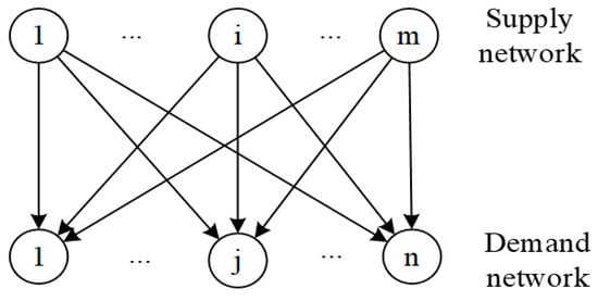
Figure 1.
Spatial price equilibrium network.
Given the practical complexity of spatial price equilibrium networks, this section proposes the following basic assumptions without altering the core of the problem:
- (1)
- All participants in the spatial price equilibrium network are “rational economic agents” who make decisions under conditions of complete information;
- (2)
- All participants in the spatial price equilibrium network have equal channel power, meaning that each supply market can trade with all demand markets, and each demand market can trade with all supply markets;
- (3)
- Supply markets produce goods through non-cooperative games, with the goods being homogeneous and mutually substitutable.
All the parameters covered in this paper are shown in Table 1.

Table 1.
Parameter definitions.
2.2. Model Building
This paper proposes a bi-level programming model designed to maximize consumer welfare, in which the government and the spatial price equilibrium network serve as the upper-level leader and lower-level follower in a Stackelberg game, as illustrated in Figure 2. This study investigates how the government can optimize the business environment in different regional supply markets through investment, thereby reducing product costs in the supply chain. Given the geographical independence of all supply markets and demand markets, reductions in product costs in supply markets will significantly impact the equilibrium state of the entire product supply chain network, thereby indirectly influencing the government’s investment allocation strategies for each supply market. The government’s objective is to improve the business environment through adjustments to these investment allocation measures to stimulate market vitality. The government’s strategic adjustments aim to achieve the optimal equilibrium of the supply chain network, maximize consumer welfare as much as possible, and thereby ultimately determine the most effective government investment allocation plan.
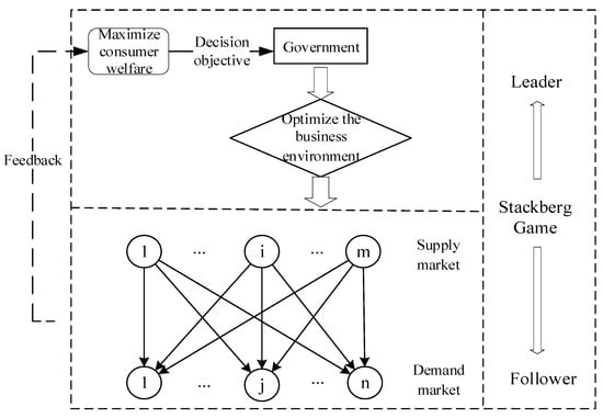
Figure 2.
Model framework.
2.3. The Upper-Level Model
Consumer surplus is an important indicator of consumer welfare; a concept derived from Marshall’s theory of marginal utility value. It refers to the difference between the highest price a consumer is willing to pay and the actual market price [1]. Consumer welfare can be divided into two categories: direct welfare and indirect welfare. Direct welfare refers to the quantifiable improvements in welfare that consumers immediately obtain from government investment, primarily measured through consumer surplus. Indirect welfare, on the other hand, refers to the long-term benefits generated by improving the overall economic environment and market structure, such as industrial agglomeration effects and innovation spillover effects.
Based on this, the government aims to enhance resource allocation efficiency through investment allocation, optimize the business environment of the product supply chain, reduce market and institutional transaction costs for business entities, thereby lowering supply prices, increasing product supply and transaction volumes, and ultimately enhancing consumers’ direct welfare. This paper focuses on direct consumer welfare, with the upper-level model aiming to maximize consumer welfare as the objective function, using numerical integration methods to calculate consumer surplus, as shown in Equation (1).
2.4. The Lower-Level Model
According to Nagurney’s theory of spatial price equilibrium, geographic factors influence the flow of goods, resulting in transportation costs that cause the price of the same product to vary across different regions [28]. If there is a positive investment flow from the investment market to the demand market, equilibrium requires that the value of the remaining investment product in the demand market must be at least equal to the supply market price plus the unit transport costs. If this condition is not met, no transaction occurs. In summary, a transaction happens only if the value of the product in the demand market is sufficient to cover the supply market price and associated costs, as expressed in Equation (2):
where Q represents the equilibrium product flow between markets under the spatial price equilibrium framework.
Since variational inequalities can describe the interactions and constraints in a system well, they are commonly used to study equilibrium problems, and the spatial price equilibrium conditions can be integrated into a variational inequality form for description. Define the vector-valued function as follows:
Substitute it into the standard variational inequality, i.e., solve such that satisfies the following inequality:
where is a feasible set and is closed and convex.
When constructing the lower-level objective function, if the Jacobi matrices of the supply price function, demand price function, and unit transport cost function are symmetric, the spatial price equilibrium condition can not only be expressed in the form of a variational inequality but also through the nonlinear optimization model of Equation (2). This nonlinear optimization model can be further solved to find the equilibrium solution under the spatial price equilibrium condition. From this solution, the corresponding supply quantity, demand quantity, supply price, demand price, and unit transport cost can be determined based on the trading volume.
where the function definitions are as follows:
Proof.
(Symmetry of Jacobi matrices for price and cost functions).
From Equation (9), the plant supply price involved in this paper is a function that is related only to its own supply, i.e., , , but , , . The Jacobi matrix of supply prices is , where the diagonal elements are , All others are zero, the Jacobi matrix of supply prices is a symmetric square matrix of order.
Similarly, from Equation (10), the demand market price of the demand market involved in this paper is a function of only the quantity demanded by itself, i.e., the Jacobi matrix of the demand price is . The Jacobi matrix of demand prices is an n-order symmetric square matrix.
As can be seen in Equation (11), the unit transport costs of the demand pairs involved in this paper are a function of the volume of transactions only between their own demand pairs, i.e., , but , ; ; ; ; do not simultaneously equal .
The Jacobi matrix for unit transport costs is , where the diagonal elements are all other elements are zero, i.e., the Jacobi matrix of unit transport costs is a symmetric square matrix of order .
Therefore, the Jacobi matrices of the supply price function, the demand price function, and the unit transport cost function are all symmetric, and the proof is complete. □
Proof.
(The nonlinear optimization model is equivalent to the spatial price equilibrium condition).
Since the objective function of the nonlinear optimization model is minimization, the nonlinear optimization model (5) is adjusted to be:
Constructing a Lagrange function as follows:
Therefore, to solve the nonlinear optimization problem, the Karush–Kuhn–Tucker condition must be satisfied:
According to the Karush–Kuhn–Tucker condition, if , then , that is ; if , then , that is . Therefore, the Karush–Kuhn–Tucker conditions are equivalent to the spatial price equilibrium conditions. The optimal solution to a nonlinear programming problem must satisfy the Karush–Kuhn–Tucker conditions and also satisfy the spatial price equilibrium conditions. Thus, the lower-level spatial price equilibrium model can be given by Equation (5), end of proof. □
2.5. The Bi-Level Programming Model
This paper investigates a bi-level programming model aimed at analyzing how governments allocate investments to enhance consumer welfare under spatial price equilibrium. The upper-level model, which aims to maximize consumer welfare, explores the mechanisms through which government investments influence the business environments of different supply markets and conducts an in-depth analysis of how differentiated investment allocation strategies impact consumer welfare. The lower-level model is a spatial price equilibrium model that reflects changes in market supply, demand, and prices under different investment intensities, and feeds back the equilibrium results into the upper-level objective function. This model achieves an organic integration of macroeconomic policies and microeconomic market responses, aiding in the formulation of more efficient government investment policies to effectively enhance consumer welfare. Therefore, the bi-level programming model can be derived as follows:
3. Solution Algorithm
3.1. Uniqueness of the Solution to the Space Price Equilibrium Condition in the Lower-Level Model
In the bi-level programming model, proving the uniqueness of the solution to the lower-level problem is essential to ensure the reliability of the algorithm’s results. This guarantees certainty for the upper-level problem and prevents increased computational complexity or reduced algorithm efficiency due to multiple solutions in the lower-level. As can be seen from Section 2.4, the spatial price equilibrium condition expressed by Equation (2) is equivalent to the variational inequality form of Equation (4) and the nonlinear programming model form of Equation (5).Therefore, by proving the existence of a unique solution to the variational inequality form, the existence of a unique solution to the lower-level spatial price equilibrium problem is established. This ensures a unique transaction volume between each supply and demand pair under the spatial price equilibrium condition.
Proof.
(Existence of a unique solution to the lower-level problem).
- (1)
- Existence of solutions
According to the existence theorem of the variational inequality, the variational inequality of Equation (4), , is the set of all non-negative transaction volumes, i.e., At the same time, since is a transaction volume, it cannot be infinitely large, i.e., there is an upper bound. Here, defined a constant such that . Therefore, the set is closed and bounded, i.e., compact. Furthermore, based on the functions and it can be concluded that and are all linear continuous functions. Since is also a continuous function. Therefore, the variational inequality form of the spatial price equilibrium condition has a solution.
- (2)
- Uniqueness of solutions
According to the uniqueness theorem of the variational inequality, for the variational inequality of Equation (4), the supply price function , and , then is a monotonically increasing function about the unit transportation cost function, where, is a monotonically increasing function about ; the demand price function , and is a monotonically decreasing function about . Combining these conditions, it can be concluded that is a monotonically increasing function about , which implies that is a strictly monotonic function. Therefore, the solution to the variational inequality for the spatial price equilibrium condition is unique.
Therefore, there exists a unique solution to the variational inequality form of the spatial price equilibrium condition, and there exists a unique solution to the lower-level spatial price equilibrium problem, and the proof is complete. □
3.2. Algorithm Process
This paper presents a bi-level programming model. The upper-level explores how the government can promote management innovation through investment, which is a continuous decision-making problem solved using a simulated annealing algorithm. The lower-level addresses the spatial price equilibrium condition, which has a unique solution and is solved using projection algorithms. For each upper-level decision, there is a corresponding unique solution at the lower-level.
Step 1: Parameter setting and variable initialization
Set all relevant parameters and function coefficients for the model. Randomly generate initial investment allocation schemes and transaction volumes.
Step 2: Upper-level simulated annealing algorithm
- (1)
- Initialize the current temperature and set the cooling coefficient to achieve a gradual decrease in temperature; randomly generate a new investment allocation plan within the neighborhood of the current solution; decide whether to accept the new solution based on its quality and the current temperature; as the iteration proceeds, gradually lower the system temperature to improve the accuracy and efficiency of the search.
- (2)
- Verify runtime conditions: If the current temperature is greater than the minimum temperature and has not reached the maximum iteration count for the current temperature, proceed to (3) to start the loop; otherwise, exit the simulated annealing algorithm, terminate the computation, and proceed to Step 5.
- (3)
- Update upper-level decision variables: Generate new business environment levels by applying small random perturbations to the current upper-level decision variables, ensuring they remain within the decision variable range, and pass the current business environment levels of all manufacturers into Step 3 for calculation.
Step 3: Lower-level projection algorithm
- (1)
- Gradient Calculation: Based on the trading volume , supply price , unit transportation cost , and demand price for each supply–demand pair , calculate the gradient , thereby obtaining the gradient of the objective function .
- (2)
- Gradient Descent: Combining the calculated gradient and update the step size, let to update the trading volume in the negative gradient direction. During this process, check the stopping criteria: if the change in objective function is smaller than the preset tolerance (i.e., the difference in objective function values between consecutive iterations is very small) or if the maximum number of iterations is reached, then stop the iteration. Meanwhile, ensure that the updated satisfies the non-negativity constraint.
- (3)
- Projection to Feasible Region: If the updated is less than 0, then project to the feasible region, setting ensuring all elements are non-negative, i.e., satisfying all and supply–demand balance constraints.
- (4)
- Price Update: Based on the updated , calculate the updated supply price and demand price .
- (5)
- Cost Update: Based on the updated , calculate the updated unit transportation cost .
- (6)
- Verification of Lower-Level Spatial Price Equilibrium Convergence Conditions: Verify based on the prices and costs of each supply–demand pair. If a supply–demand pair has trading, satisfying is considered to have reached equilibrium; if a supply–demand pair has no trading, satisfying is considered to have reached equilibrium. When every supply–demand pair satisfies the above conditions, proceed to Step 4; otherwise, return to (2) to continue iteration.
Step 4: Upper-level iterative solution
Based on the lower-level equilibrium solution of the current investment allocation decision, calculate the upper-level objective function. If the current consumer welfare is better than the historical optimal consumer welfare, update the optimal solution and the corresponding optimal investment allocation decision, and return to Step 2 for the simulated annealing algorithm. Otherwise, no update is needed, and return directly to Step 2.
Step 5: Output results
Output the final upper-level optimal solution and the corresponding lower-level transaction volume, supply price, demand price, and unit transportation cost.
The basic steps of the algorithm have been described in detail in the preceding text. To illustrate the overall process and structure of the algorithm more clearly and intuitively, this paper further provides the algorithm framework diagram shown in Figure 3. This diagram helps readers better understand the logical relationships and execution order among the various modules.
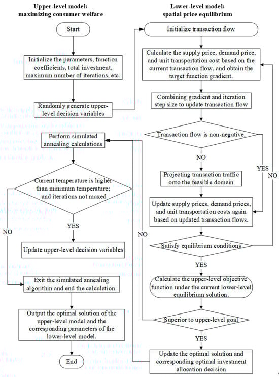
Figure 3.
Flowchart of bi-level programming algorithm.
Figure 3 not only shows the overall framework of the algorithms but also clearly depicts the interactions among the steps, visualizing how the two algorithms work together to efficiently solve the bi-level programming model problem.
4. Experimental Study
4.1. Illustrative Case
Figure 4 is a simplified example diagram of a spatial price equilibrium network under a government investment allocation decision-making framework. The network structure primarily consists of three supply markets and three demand target markets distributed across different regions, forming a typical many-to-many supply–demand matching pattern. The solid nodes at the top represent government investment, while the dashed nodes at the bottom indicate consumer welfare. Within this bi-level optimization framework, the government, as the upper-level decision-maker, improves the business environment in each region by optimizing investment allocation strategies, thereby reducing market transaction costs. Simultaneously, it must consider spatial price equilibrium constraints and social welfare impact mechanisms to formulate a reasonable investment allocation plan aimed at maximizing consumer welfare. The transaction unit for products is kilograms. The supply price functions of different supply markets, the demand price functions of different demand markets, and the unit transportation cost functions between different supply–demand pairs vary because of their own influences. Prices are denominated in USD, and costs are denominated in USD per kilogram.
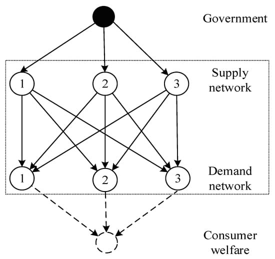
Figure 4.
Government investment and spatial price equilibrium network interaction diagram.
The supply price functions for each of the original three supply markets in this example are:
The demand price functions for each of the three demand markets are:
The unit transportation cost functions between the original supply and demand pairs are, respectively:
The total investment amount is , and the other parameters are:
The relevant parameters and functions were substituted into the bi-level programming model and calculated using RStudio (2022.07.2+576). The equilibrium production, transportation, and consumption model are given by the following:
Equilibrium supply prices, transaction costs, and demand prices:
At this point, the investment amounts in each of the three supply markets are The levels of the business environment are, respectively, . The final consumer welfare is
4.2. Sensitivity Analysis
In this calculation example, it is assumed that the government optimizes the local business environment by continuously increasing investment, although the amount of increased investment is subject to certain limitations and constraints. In this example, we analyze the changes in consumer welfare as the government gradually increases the total investment from one million one hundred thousand USD to two million USD in increments of one hundred thousand USD. For the convenience of table presentation, investment amounts are uniformly expressed in 10,000 USD increments. Here, the rate of change in consumer welfare is calculated as the difference between consumer welfare at the subsequent level of investment and consumer welfare at the previous level of investment, divided by the consumer welfare at the previous level of investment. The detailed numerical results are presented in Table 2 below.
Table 2.
Consumer welfare at different total investment amounts.
According to Table 2, with the increase in total investment, the three supplying cities experience significant changes in the amount of investment received and the level of business environment. Observing the rate of change in business benefits, it is found that the rate of change is particularly high at 0.0019 and 0.0025 when the total investment reaches 1.4 million USD and 1.9 million USD, respectively. Meanwhile, the rate of change in consumer welfare turns negative when the total investment is 1.6 million USD, 1.8 million USD, and 2.0 million USD, indicating a reduction in consumer welfare at these levels. The relationship between the business environment and total investment is depicted in a line graph, as shown in Figure 5 below.
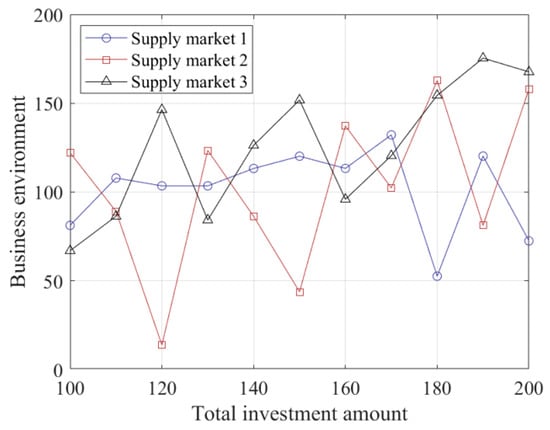
Figure 5.
Business environment at different total investment amounts.
As shown in Figure 5, the business environment in the three supply markets exhibits distinct nonlinear fluctuations in response to changes in total investment amounts. Supply Market 1 demonstrates relative stability with minimal fluctuations; supply market 2 exhibits the most significant fluctuations, with the business environment deteriorating sharply at certain investment levels but improving significantly as investment increases; supply market 3 performs the best overall, with the business environment index typically maintaining a high level. These differentiated patterns of change indicate that simply increasing the total investment amount does not guarantee simultaneous improvements in the business environments of all supply markets. Instead, it is necessary to develop differentiated investment allocation strategies tailored to the specific characteristics and sensitivities of each market to achieve overall optimization of the business environment. To better illustrate these changes, the relationship between consumer welfare and total investment is depicted in a line graph, as shown in Figure 6 below.
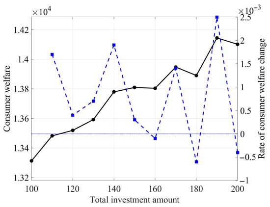
Figure 6.
Consumer welfare at different total investment amounts.
As shown in Figure 6, consumer welfare generally exhibits an increasing trend as total investment amounts grow, but the growth process is not smooth and instead exhibits distinct phased characteristics. The rate of change in consumer welfare exhibits significant fluctuations, with notable positive growth at certain investment levels and potential negative growth at others. The analysis of data in Table 2 reveals that when the total investment amount reaches 1.9 million USD, the rate of change in consumer welfare reaches a relatively high level, at which point consumer welfare achieves an optimal state. At this point, the investment amounts for the three supply markets are respectively. The levels of the business environment are , while the consumer welfare is .
Based on the above analysis, it is recommended that the total investment scale be controlled within a reasonable range in actual investment decisions to avoid blindly increasing investment. At the same time, differentiated resource allocation should be carried out among multiple supply markets, with a focus on investing in markets with higher efficiency. An investment effectiveness evaluation system should also be established to promptly adjust investment strategies when consumer welfare growth rates show a downward trend, thereby maximizing the utilization of limited resources and optimizing consumer welfare.
5. Conclusions
This paper aims to explore the role of government in promoting investment allocation to maximize business environment development and enhance consumer welfare. To achieve this, a bi-level programming model is constructed, where the upper-level model seeks to maximize consumer welfare, and the lower-level model addresses the spatial price equilibrium network. To ensure the model’s effectiveness and feasibility, a hybrid solution approach is employed, integrating simulated annealing and gradient projection algorithms.
The results indicate that the bi-level programming model systematically analyzes the impact of various investment allocation decisions on the spatial price equilibrium network. This approach not only enriches the theoretical framework of government investment allocation and supply chain management but also enhances the model’s alignment with real-world economic operations by integrating business environment factors alongside transportation costs and transaction volume equilibrium. Sensitivity analysis further reveals that increasing the intensity of investment allocation and the total investment amount can significantly improve consumer welfare, thereby providing support for the government to scientifically determine investment scales and optimize the business environment. Consequently, this study recommends that governments tailor business environment optimization strategies to the resource endowments and development stages of each region, ensuring effective improvements in consumer welfare.
Nonetheless, this study has certain limitations that warrant further exploration. First, real-world product transportation in reality often involves the risk of losses, and spatial price equilibrium issues require consideration of more complex factors, such as the dynamic impact of external factors, such as economic shocks and policy changes, on market equilibrium. Second, the business environment encompasses a wide range of factors, including not only direct investment measures such as infrastructure development and fiscal subsidies but also multidimensional aspects such as institutional frameworks, regulatory policies, and tax systems. The synergistic effects of these factors can alter the lower-level spatial price equilibrium solution, thereby influencing consumer welfare in the upper-level. Finally, uncertainties in investment and the business environment (such as fluctuations in market demand, technological changes, and policy adjustments) can substantially impact the applicability of the model.
To address these limitations, future research will explore the following directions: (1) a dynamic extension model can be developed by incorporating a multi-stage stochastic programming framework, where critical parameters such as demand, costs, and policies are modeled as stochastic processes to better account for uncertain environments. (2) Considering diversified business environment optimization strategies comprehensively, transcending the single perspective of investment allocation; (3) Analyzing the mechanisms through which external uncertainties affect model stability and policy effectiveness. Through these extensions, synergistically driving business environment construction and consumer welfare improvement will further enhance regional competitiveness and promote local economic sustainable development.
Author Contributions
Conceptualization, methodology, investigation, validation, writing—original draft, data curation, software, T.X.; conceptualization, methodology, writing-review and editing, resources, funding acquisition, supervision, software, H.L. All authors have read and agreed to the published version of the manuscript.
Funding
This research is supported by the General Program of the National Social Science Foundation (Grants No. 24BGL238).
Data Availability Statement
No new data were created or analyzed in this study. Data sharing is not applicable to this article.
Acknowledgments
The authors wish to thank the anonymous reviewers for their suggestions, which were very useful in revising the paper.
Conflicts of Interest
No potential conflicts of interest were reported by the authors.
References
- Marshall, A. Principles of Economics; Commercial Press: Beijing, China, 1985. [Google Scholar]
- Chen, Y.H.; Wen, X.W.; Wang, B.; Nie, P.Y. Agricultural pollution and regulation: How to subsidize agriculture? J. Clean. Prod. 2017, 164, 258–264. [Google Scholar] [CrossRef]
- Yu, J.J.; Tang, C.S.; Shen, Z.J.M. Improving consumer welfare and manufacturer profit via government subsidy programs: Subsidizing consumers or manufacturers? Manuf. Serv. Oper. Manag. 2018, 20, 752–766. [Google Scholar] [CrossRef]
- Kalvin, B.; Pau, C. The impact of spectrum assignment policies on consumer welfare. Telecommun. Policy 2022, 46, 102228. [Google Scholar] [CrossRef]
- Nugrahapsari, R.A.; Hasibuan, A.M.; Novianti, T. Impacts of trade policy on the welfare of citrus producers and consumers in Indonesia. Int. J. Soc. Econ. 2024, 51, 1278–1297. [Google Scholar] [CrossRef]
- He, C.; Zhou, C.; Wen, H. Improving the consumer welfare of rural residents through public support policies: A study on old revolutionary areas in China. Socio-Econ. Plan. Sci. 2024, 91, 101767. [Google Scholar] [CrossRef]
- Zhang, Y.; Lu, X.; Xiao, J. Can financial education improve consumer welfare in investment markets? Evidence from China. J. Asia Pac. Econ. 2023, 28, 1286–1312. [Google Scholar] [CrossRef]
- Kreuter, H.; Riccaboni, M. The impact of import tariffs on GDP and consumer welfare: A production network approach. Econ. Model. 2023, 126, 106374. [Google Scholar] [CrossRef]
- Kang, W.; Shao, B. The impact of voice assistants’ intelligent attributes on consumer well-being: Findings from PLS-SEM and fsQCA. J. Retail. Consum. Serv. 2023, 70, 103130. [Google Scholar] [CrossRef]
- Ash, D.; Ben Shahar, D. Zero-price effect and consumer welfare: Evidence from online classified real estate service. Real. Estate Econ. 2024, 5, 1165–1196. [Google Scholar] [CrossRef]
- Yoon, J.; Matsumura, M.; Weinstein, D.E. The Impact of Retail E-Commerce on Relative Prices and Consumer Welfare. Rev. Econ. Stat. 2024, 6, 1675–1689. [Google Scholar] [CrossRef]
- Li, Z. 2020 Evaluation of Doing Business in Chinese Cities; China Development Press: Beijing, China, 2021. [Google Scholar]
- Du, Y.Z.; Liu, Q.C.; Cheng, J.Q. What kind of business environment ecosystem produces high urban entrepreneurial activity?—Analysis based on institutional configuration. J. Manag. World. 2020, 36, 141–155. [Google Scholar]
- Nagurney, A.; Daniele, P.; Shukla, S. A supply chain network game theory model of cybersecurity investments with nonlinear budget constraints. Ann. Oper. Res. 2017, 248, 405–427. [Google Scholar] [CrossRef]
- Nagurney, A.; Shukla, S. Multifirm models of cybersecurity investment competition vs. cooperation and network vulnerability. Eur. J. Oper. Res. 2017, 260, 588–600. [Google Scholar] [CrossRef]
- Nagurney, A.; Shukla, S.; Nagurney, L.S.; Saberi, S. A game theory model for freight service provision security investments for high-value cargo. Econ. Transp. 2018, 16, 21–28. [Google Scholar] [CrossRef]
- Nagurney, A. Optimization of supply chain networks with inclusion of labor: Applications to COVID-19 pandemic disruptions. Int. J. Prod. Econ. 2021, 235, 108080. [Google Scholar] [CrossRef] [PubMed]
- Xu, M.; Anupriya, B.; Bansal, P. Surge pricing and consumer surplus in the ride-hailing market: Evidence from China. Travel Behav. Soc. 2023, 33, 100638. [Google Scholar] [CrossRef]
- Huh, W.T.; Li, H. Product-line pricing with dual objective of profit and consumer surplus. Prod. Oper. Manag. 2023, 32, 1223–1242. [Google Scholar] [CrossRef]
- McHardy, J.; Reynolds, M.; Trotter, S. A consumer surplus, welfare and profit enhancing strategy for improving urban public transport networks. Reg. Sci. Urban Econ. 2023, 100, 103899. [Google Scholar] [CrossRef]
- Vicente, L.N. Bi-level and multi-level programming: A bibliography review. J. Glob. Optim. 1994, 5, 291–306. [Google Scholar] [CrossRef]
- Migdalas, A.; Padalos, P.M.; Varbrand, P. Multi-Level Optimization: Algorithms and Applications; Kluwer Academic: London, UK, 1997. [Google Scholar]
- Candler, W.; Norton, R. Multi-Level Programming; World Search: Washington, DC, USA, 1977. [Google Scholar]
- Kleinert, T.; Labbé, M.; Ljubić, I.; Schmidt, M. A survey on mixed-integer programming techniques in bilevel optimization. EURO J. Comput. Optim. 2021, 9, 100007. [Google Scholar] [CrossRef]
- Bracken, J.; McGill, J.T. Mathematical programs with optimization problems in the constraints. Oper. Res. 1973, 21, 37–44. [Google Scholar] [CrossRef]
- Tantiwattanakul, P.; Dumrongsiri, A. Supply chain coordination using wholesale prices with multiple products, multiple periods, and multiple retailers: Bi-level optimization approach. Comput. Ind. Eng. 2019, 131, 391–407. [Google Scholar] [CrossRef]
- Parsa, S.P.; Allah, A.T.; Eduardo, L.B.C. Retail price competition of domestic and international companies: A bi-level game theoretical optimization approach. RAIRO-Oper. Res. 2023, 57, 291–323. [Google Scholar] [CrossRef]
- Nagurney, A. Network Economics: A Variational Inequality Approach; Kluwer Academic: Dordrecht, The Netherlands, 1999. [Google Scholar]
Disclaimer/Publisher’s Note: The statements, opinions and data contained in all publications are solely those of the individual author(s) and contributor(s) and not of MDPI and/or the editor(s). MDPI and/or the editor(s) disclaim responsibility for any injury to people or property resulting from any ideas, methods, instructions or products referred to in the content. |
© 2025 by the authors. Licensee MDPI, Basel, Switzerland. This article is an open access article distributed under the terms and conditions of the Creative Commons Attribution (CC BY) license (https://creativecommons.org/licenses/by/4.0/).