Finite-Time Tracking Control in Robotic Arm with Physical Constraints Under Disturbances

Abstract

This paper proposes a novel control algorithm for robotic manipulators with unknown nonlinearities and external disturbances. Explicit consideration is given to the physical constraints on joint positions and velocities, ensuring tracking performance without violating prescribed constraints. Finite-time convergence entails significant overshoot magnitudes. A class of nonlinear transformations is employed to ensure state constraint satisfaction while achieving prescribed tracking performance. The command filtered backstepping is employed to circumvent issues of “explosion of terms” in virtual controls. A disturbance observer (DOB), constructed via radial basis function neural networks (RBFNNs), effectively compensates for nonlinearities and time-dependent disturbances. The proposed control law guarantees finite-time stability while preventing position/velocity violations during transients. Simulation results validate the effectiveness of the proposed approach.

1. Introduction

With the development of robotic technology, robotic manipulators have been widely applied in industrial manufacturing, agriculture, healthcare, and other fields. The tasks performed by robotic manipulators are increasingly diverse and complex [1,2,3]. The physical movement limitations of the robotic manipulators, the surrounding environment and the task requirements can be transformed into constraints on the angles and angular velocities of the joints [1,4,5,6,7]. If these constraints are ignored during the design process of the control algorithm, it might lead to performance degradation, safety problems, or even fatal accidents [6,7]. Therefore, it is necessary to design a tracking control algorithm that considers the joint position and the speed constraints of the joints.

For nonlinear systems (including uncertain robotic manipulators), there are some classic control methods for dealing with constraints, such as model predictive control (MPC) [8], reference governors (RG) [9], and extremum-seeking control (ESC) [10]. MPC requires solving a finite time-domain optimization problem at each sampling moment. However, for nonlinear systems and multi-state constraints, the optimization problem may be overly complex, and the solution process is extremely time-consuming. RG modifies the reference signal to ensure that the original signal does not violate the given constraints. For this purpose, a conservative set needs to be calculated in advance, which depends on the given constraints. However, the set can be sufficiently rough. ESC indirectly affects the state by optimizing the shape of the objective function. However, the constrained state may violate the constraint and, after a period, be pulled back into the constraint by the control signal.

Recently, barrier Lyapunov function (BLF) or integral BLF (IBLF)-based adaptive control schemes have been developed to address output/state constraints in nonlinear systems [1,3,11,12,13,14,15,16,17,18,19]. The backstepping is often used to design control laws for control systems with strict feedback [20]. Command filtered backstepping provides two filters. One (here, the filter can be either first-order or second-order) is used as a fast-dynamic subsystem to track the virtual controller and avoids “explosion of terms”. The other is error compensation to facilitate the proof of closed-loop system performance using the Lyapunov method [21,22]. BLF or IBLF is highly suitable for designing high-order full-state constraint control laws in combination with command filtered backstepping. In each step, introduce them. If there are state-dependent uncertain functions in the current step, RBFNNs can be used for estimation. In [1] an adaptive fuzzy finite-time singular perturbation control was proposed for flexible joint manipulators with state constraints. Model uncertainties and unknown external disturbances are handled by adaptive fuzzy technique. In [18] a finite-time tracking control for a class of strict-feedback nonlinear systems involving state constraints, unknown nonlinearities, and nonvanishing disturbances was proposed. However, in the BLF-based backstepping design process, the virtual control signal is required to satisfy a preset feasible region (also called the feasible condition) [23], which is dynamically shaped by the state constraint. This substantially complicates the parameter design process, necessitating cumbersome offline computation to verify the feasibility conditions, demanding additional time and costs in control design and implementation. Even worse, when constraint boundaries are stringent, optimal parameters fulfilling the feasible conditions may prove elusive, ultimately rendering the constrained control scheme break down precisely when tight restrictions apply.

Nonlinear mapping (NP) technique circumvents the feasible conditions. In [23], a neuroadaptive tracking control approach for uncertain robotic manipulators subject to asymmetric yet time-varying full-state constraints without involving feasibility conditions was proposed. In [23,24,25,26,27], the NP technique was leveraged to transform the problem with state constraints into a stability problem without constraints in a new coordinate. NP employs different coordinate transformations at each step of backstepping design, resulting in a control scheme that is able to circumvent the feasibility conditions, facilitating the design, and implementation of the control scheme. However, in these designs, external disturbances were not accounted for, which can compromise the tracking performance in robotic systems.

Since the initial state of the system differs from the given tracking signal, ensuring finite-time tracking is of great significance. In [1], a finite-time controller was introduced to improve the response speed of the rigid subsystem so that it can converge within a finite time. In [28], to enable the tracking error of robotic manipulator system with uncertainties to converge within finite time, a novel finite-time non-singular robust control approach was proposed. In [29], a finite-time integral terminal sliding mode control integrated with a finite-time extended state observer was proposed. However, the rapid convergence of the system may result in excessive overshoot. An excessive pursuit of convergence performance may result in instability or even system collapse. In addition, the fractional term in the Lyapunov function only dominates its transition process, and the steady-state performance of the controller cannot be guaranteed. Therefore, enhancing system performance while ensuring rapid system convergence is a worthwhile consideration.

In this paper, we propose a NP-based adaptive finite-time control for robotic manipulators with asymmetric yet time-varying state constraints. The main features and contributions of this paper can be summarized as follows.

• In contrast to [1,3,11,12,13,14,15,16,17,18,19], this study employs a specific class of NP functions (also called nonlinear transformations) to design the control law, which deals with the asymmetric yet time-varying position and velocity constraints without involving feasibility conditions. Compared with traditional methods [8,9,10], the states are always within the given constraints, without solving complex optimization problems. The states can approach the constraint boundaries arbitrarily.
• NP is also used in the framework of finite time control to ensure the given tracking quality. The transient and steady-state performance of the tracking errors are improved. Meanwhile, the other system signals converge within a finite time under different initial conditions.
• Different from [23,24,25,26,27], DOB, constructed via RBFNN, is employed to estimate signal uncertainty and functional uncertainty.

The rest of this paper is organized as follows. Section 2 presents notations, essential lemmas and the control objective. In Section 3, the uncertainty estimation method for the system is first introduced. Then, NP is used for coordinate transformation to ensure that the state constraints are not violated and the given tracking performance. Subsequently, the finite-time control law is designed using command filtered backstepping under the new coordinates. Finally, the stability analysis of the closed-loop system is conducted. Section 4 provides a simulation example to validate the proposed control approach. Finally, concluding remarks are given in Section 5.

2. Preliminaries and Problem Formulation

2.1. Notations and Key Lemmas

The following notation will be used throughout the paper:

• ${\mathbb{R}}^n$ is Euclidean space of dimension $n$ with norm $‖\cdot ‖$.
• ${\mathbb{R}}^{n\times n}$ denotes the space of $m\times n$ real matrices with the Frobenius norm ${‖\cdot ‖}_{\mathrm{F}}$.
• $0_{n,m},$ denotes the zero matrix (of the corresponding dimension).
• For quadratic matrices $M\in {\mathbb{R}}^{n\times n},M\succ 0(M\prec 0)$ means that $M$ is a positive-definite matrix (negative-definite matrix).
• $\underset{\_}{\mathsf{\sigma }}(\cdot )$ or $\overline{\mathsf{\sigma }}(\cdot )$ represents the maximum or minimum singular value of matrix.
• $tr(\cdot )$ is the trace of matrix.

The following well-known lemmas will be used to prove the main result of paper.

Lemma 1 

([30]). If $0<p=p_1/p_2<1$, where  $p_1$ and $p_2$  are positive odd integers, then there exist  $a$  and  $b\in \mathbb{R}$  satisfying the following inequality:

$$a{b}^p\le -l_1{a}^{1+p}+l_2(a+b{)}^{1+p},$$

where $l_1={\displaystyle \frac{1}{1+p}}\left(2^{p-1}-2^{(p-1)(p+1)}\right)$ and $l_2={\displaystyle \frac{1}{1+p}}\left({\displaystyle \frac{1+2p}{1+p}}+{\displaystyle \frac{2^{-(p-1{)}^2(p+1)}}{1+p}}-2^{p-1}\right)$.

Consider the following nonlinear system:

$$\dot{x}=f\left(x,t\right), x\left(t_0\right)=x_0,$$

where $x\in \Omega \subset {\mathbb{R}}^n$ is the system state, $\Omega$ is the domain, and the nonlinear function $f(x,t)$: $\Omega \times {\mathbb{R}}_{+}\to {\mathbb{R}}^n$ satisfies the local Lipschitz condition. Assume $x=0$ is the equilibrium point of the system, denoted as $x_0$, i.e., $f\left(0,t_0\right)=0$.

Lemma 2 

([31]). For the above system, if there exists a $C^1$ Lyapunov function  $V(x)\ge 0$  such that  $\dot{V}(x)\le -\alpha V^{{\displaystyle \frac{p+1}{2}}}(x)-\beta V(x)+\Delta$, where  $\alpha >0, \beta >0, 0<{\displaystyle \frac{p+1}{2}}<1$, and  $0<\Delta <\infty$, then the system is practically finite-time stable, with the settling time given by:

$$T≔max\left\{{\displaystyle \frac{\mathit{ln}\left(\frac{\alpha \rho V^{1-\frac{p+1}{2}}\left(0\right)+\beta }{\beta }\right)}{\alpha \rho \left(1-\frac{p+1}{2}\right)}},{\displaystyle \frac{\mathit{ln}\left(\frac{\alpha V^{1-\frac{p+1}{2}}\left(0\right)+\rho \beta }{\rho \beta }\right)}{\alpha \left(1-\frac{p+1}{2}\right)}}\right\}.$$

Here $0<\rho <1$ is a constant.

Remark 1. 

Lemma 1 is frequently employed to derive Lyapunov differential inequalities for establishing stability criteria that guarantee finite-time stability. Lemma 2 provides a settling time that depends on the system’s initial condition $V\left(0\right)$ and multiple design parameters of the controller.

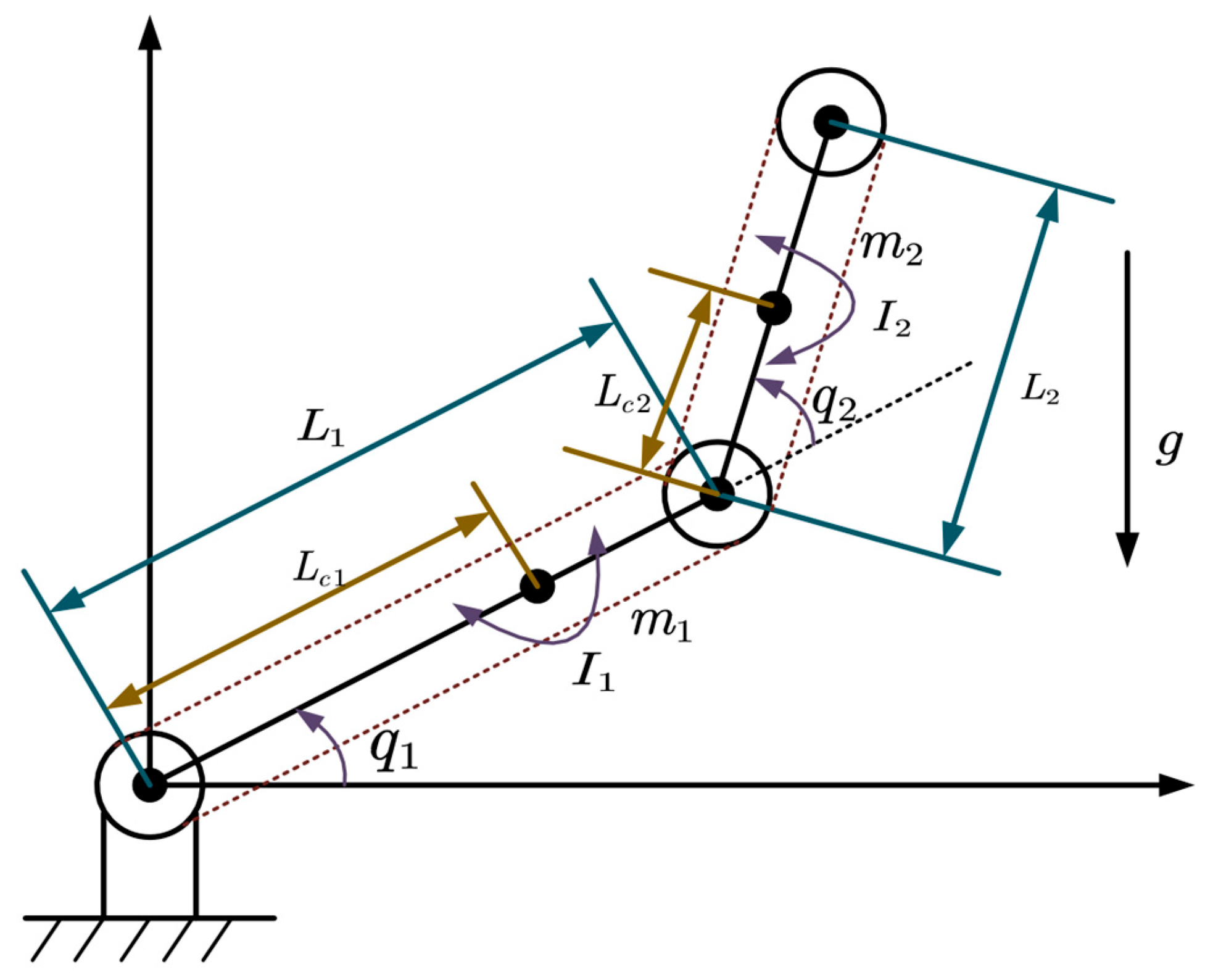
2.2. Problem Formulation

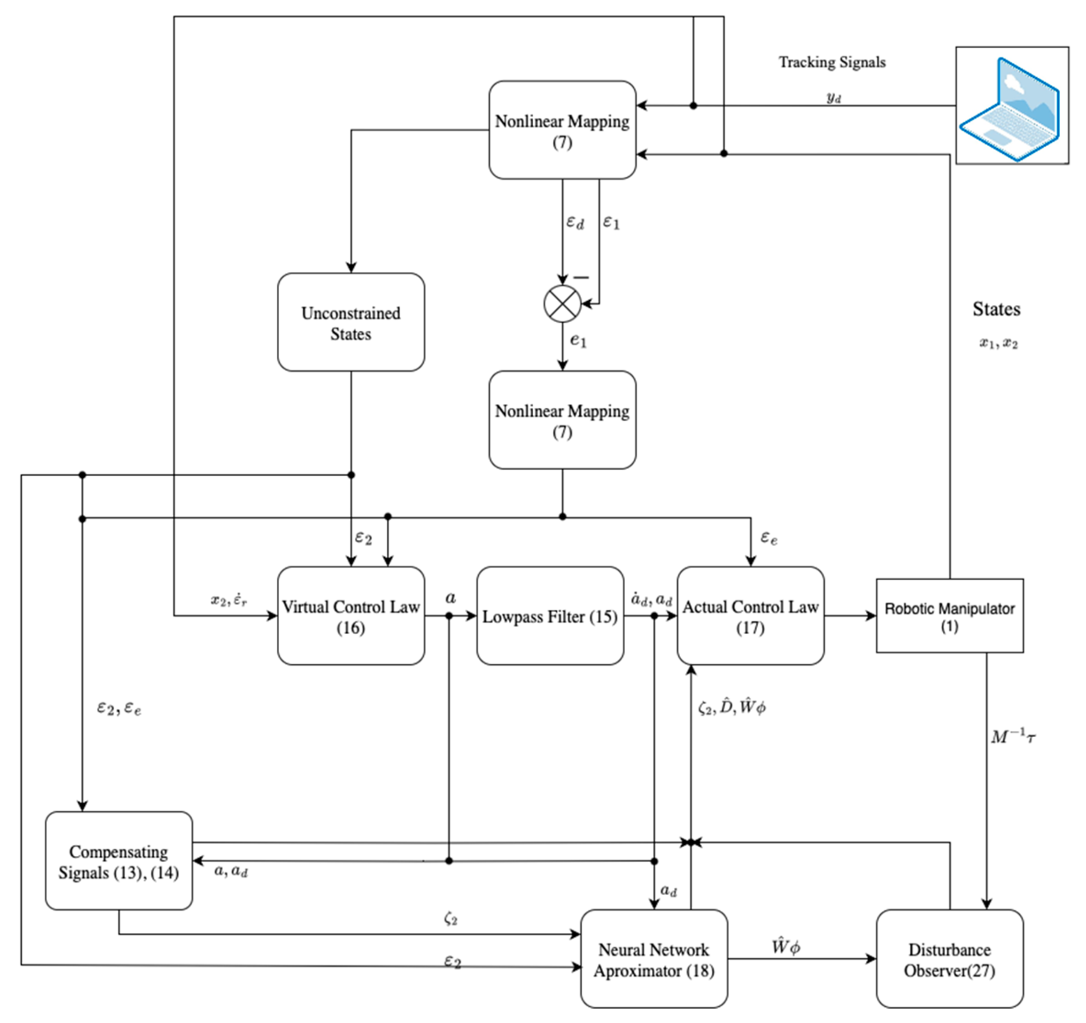
The dynamics of an $n$ degree-of-freedom (DOF) robotic manipulator can be described as a MIMO nonlinear system as follows [3,4]:

$$M\left(q\right)\ddot{q}+C\left(q,\dot{q}\right)\dot{q}+G\left(q\right)=\tau +d$$

(1)

where $q\in {\mathbb{R}}^n$ is the joint position, $M\left(q\right)\in {\mathbb{R}}^{n\times n}$ is the inertia matrix and $M\left(q\right)\succ 0$, $C(q,\dot{q})\dot{q}\in {\mathbb{R}}^n$ is the Coriolis and centrifugal force, $G\left(q\right)\in {\mathbb{R}}^n$ is the gravitational force, $d\left(q,t\right)\in {\mathbb{R}}^n$ is the unknown term including external disturbances and the joint position. $\tau \in {\mathbb{R}}^n$ is the input joint torque. $d\left(q,t\right)={f_r}^T\left(q\right){\phi }_r\left(t\right)$, ${\phi }_r\left(t\right)\in {\mathbb{R}}^n$ is the unknown vector of external disturbances, $f_r\left(q\right)\in {\mathbb{R}}^{n\times n}$ is the unknown reversible Jacobean matrix. Take a two-link robotic manipulator as an example: Figure 1 depicts its kinematic structure, with primary geometric and inertial parameters provided in

Table 1. Primary parameters.

Symbol	Description	Unit
$q_1,q_2$	Angular positions of links 1 and 2	rad
$m_1,m_2$	Masses of links 1 and 2	kg
$L_1,L_2$	Link lengths	$\mathrm{m}$
$L_{c1},L_{c2}$	Centroid offset distances from joints	$\mathrm{m}$
$I_1,I_2$	Linear momenta of links	$\mathrm{k}\mathrm{g}.{\mathrm{m}}^2$
$g$	Gravity acceleration	$\mathrm{m}/{\mathrm{s}}^2$

. Define that $q=x_1={\left[x_{11},\dots ,x_{1n}\right]}^T\in {\mathbb{R}}^n$ and $\dot{q}=x_2=$ ${\left[x_{21},\dots ,x_{2n}\right]}^T\in R^n$, then (1) can be expressed as

$$\left\{\begin{array}{c}{\dot{x}}_1=x_2,\\ {\dot{x}}_2=M^{-1}\left(\tau -C{x}_2-G+d\right).\end{array}\right.$$

(2)

In this paper, we consider two typical motion constraints, i.e., position and velocity constraints.

$${\underset{\_}{g}}_{1,i}<q_i<{\bar{g}}_{1,i},{\underset{\_}{g}}_{2,i}<{\dot{q}}_i<{\bar{g}}_{2,i}$$

(3)

for $i=\mathrm{1,2},\dots ,n$, where ${\underset{\_}{g}}_{k,i} \mathrm{a}\mathrm{n}\mathrm{d} {\bar{g}}_{k,i}$($k=1, 2$) are known constants or time-varying limits.

The objective of this paper is to design a control law that ensures the system states $x_1$ track a given reference trajectory $y_d(t)={\left[y_{d1},\dots ,y_{dn}\right]}^T$ within finite time $T$ with minimal achievable error, while guaranteeing no violation of constraint (3) and the given tracking quality. To guarantee the fulfillment of the objective, we introduce the following assumptions:

Assumption 1. 

The initial position and velocity satisfy ${\underset{\_}{g}}_{1,i}<q_i(0)<{\bar{g}}_{1,i}$ and ${\underset{\_}{g}}_{2,i}<{\dot{q}}_i(0)<{\bar{g}}_{2,i}$ for $i=\mathrm{1,2},\dots ,n$.

Assumption 2. 

The external disturbance $d$ and  $\dot{d}$ are bounded, the reference signals  $y_d$,  ${\dot{y}}_d$  are bounded.

Assumption 3. 

The inertia matrix $M\left(q\right)$ is measurable, whereas the Coriolis  $C\left(q,\dot{q}\right)$  and centrifugal terms  $G\left(q\right)$  are unknown.

3. Main Results

3.1. DOB Design via RBFNNs

Neural Networks (NNs) are widely employed in nonlinear system control and modeling due to their superior function approximation, learning, and fault tolerance capabilities. Among various NN architectures, RBFNNs are particularly favored for their simple structure and linear parameterization. In this work, we utilize RBFNNs to approximate the nonlinear component $M^{-1}\left(-{Cx}_2-G\right)$ in Equation (2) over the compact set ${\Omega }_Z\subseteq {\mathbb{R}}^{2n}$, defined as follows:

$$M^{-1}\left(-{Cx}_2-G\right)=W^T\varphi \left(Z\right)+\delta \left(Z\right),$$

(4)

where $Z={\left[x_{11},\dots ,x_{1n},x_{21},\dots ,x_{2n}\right]}^T$; $W=\left[\begin{array}{ccc}{w}_1& \dots & 0_{l\times 1}\\ ⋮& \ddots & ⋮\\ 0_{l\times 1}& \dots & w_n\end{array}\right]$, $w_i\in {\mathbb{R}}^l ,$ are is the optimal weight vectors of RBFNNs, $l$ is the number of neuron; $\delta ={\left[{\delta }_1,\dots ,{\delta }_n\right]}^T$ is the approximation error; $\varphi \left(Z\right)={\left[{\varphi }_1^T\left(Z\right),\dots ,{\varphi }_n^T\left(Z\right)\right]}^T$ is a known smooth basis function vector; ${\varphi }_i\left(Z\right)={\left[{\varphi }_{1,i}\left(Z\right),\dots ,{\varphi }_{l,i}\left(Z\right)\right]}^T$, ${\varphi }_{j,i}\left(Z\right)\in \mathbb{R}\left(j=1,\dots ,l\right)$ is chosen as the commonly used Gaussian function with the form: ${\varphi }_{j,i}\left(Z\right)=$ $\mathrm{e}\mathrm{x}\mathrm{p}\left[-\left({\left(Z-{\varpi }_{j,i}\right)}^T\left(Z-{\varpi }_{j,i}\right)\right)/{\varrho }_{j,i}^2\right]$, where ${\varpi }_{j,i}\in {\mathbb{R}}^{2n}$ denotes the center of the receptive field; ${\varrho }_{j,i}$ represents the width of the Gaussian function.

Remark 2. 

As recommended in [32,33], the selection of RBFNNs should adhere to the following principle: By increasing the number of neurons and appropriately choosing centers ${\varpi }_{j,i}$ and widths ${\varrho }_{j,i}$, the approximation error $\delta \left(Z\right)$ can be bounded by any $\overline{\delta }>0$ over the compact set ${\Omega }_Z$, here $\overline{\delta }$ is a positive constant. For Gaussian basis functions, $\left|{\varphi }_{j,i}\right(\cdot \left)\right|\le 1$.

Remark 3. 

In many works [3,4,6], the optimal weights of RBFNNs are often assumed to be bounded. In this work, we make the same assumption such that ${‖W‖}_F\le W_M$.

By integrating Equation (4) with the disturbance observer proposed in [34], the second expression in (2) is reformulated as:

$${\dot{x}}_2=M^{-1}\tau +W^T\varphi +D,$$

(5)

where $D=\delta \left(Z\right)+M^{-1}d$ denotes total disturbance of the robotic system including the estimation error of RBFNNs and the external disturbances. The total disturbance can be compensated by the following DOB:

$$\left\{\begin{array}{c}{\gamma }^{-1}\widehat{D}=x_2-\xi ,\\ \dot{\xi }={\widehat{W}}^T\varphi +M^{-1}\tau +\widehat{D}-k_1{\gamma }^{-1}{\widehat{D}}^p,\end{array}\right.$$

(6)

where $\widehat{W}=\left[\begin{array}{ccc}{\widehat{w}}_1& \dots & 0_{l\times 1}\\ ⋮& \ddots & ⋮\\ 0_{l\times 1}& \dots & {\widehat{w}}_n\end{array}\right]$ is the estimate of $W$; $\widehat{D}={\left[{\widehat{D}}_1,\dots ,{\widehat{D}}_n\right]}^T,$ ${\widehat{D}}_i\in \mathbb{R}$ is the estimate of $D$, $\gamma >0, k_1>0$ are constants; $\xi ={\left[{\xi }_1,\dots ,{\xi }_{\mathrm{n}}\right]}^T$, ${\xi }_i\in \mathbb{R}$ is an intermediate vector of the DOB.

3.2. Nonlinear Mapping

Let us consider a NP of the vector $x_k\left(t\right)$ in the form [35,36]:

$$x_k\left(t\right)={\mathsf{\Phi }}_k\left({\epsilon }_k\left(t\right),t\right),$$

(7)

where ${\epsilon }_k\left(t\right)\in {\mathbb{R}}^n$ is the continuously differentiable vector function for all $t$, the function ${\mathsf{\Phi }}_k({\epsilon }_k,t)=\mathrm{c}\mathrm{o}\mathrm{l}\left\{{\mathsf{\Phi }}_{k,1}({\epsilon }_{k,1},t),\dots ,{\mathsf{\Phi }}_{k,n}({\epsilon }_{k,n},t)\right\}$ satisfies the following conditions:

(a).

${\underset{\_}{g}}_{k,i}(t)<{\mathsf{\Phi }}_{k,i}({\epsilon }_{k,1},t)<{\bar{g}}_{k,i}(t),$ for all $t\ge 0$;

(b).

${\mathsf{\Phi }}_k\left({\epsilon }_k\right(t),t)$ is a continuously differentiable function and ${\displaystyle \frac{\partial {\mathsf{\Phi }}_k({\epsilon }_k,t)}{\partial {\epsilon }_k}}\succ 0 \mathrm{for} \mathrm{any} t\ge 0 \mathrm{and} {\epsilon }_k\in {\mathbb{R}}^n;$

(c).

${\displaystyle \frac{\partial {\mathsf{\Phi }}_k\left({\epsilon }_k\right(t),t)}{\partial t}}$ is bounded function on $t\ge 0$ for all ${\epsilon }_k\in {\mathbb{R}}^n$.

Here ${\displaystyle \frac{\partial {\mathsf{\Phi }}_k({\epsilon }_k,t)}{\partial {\epsilon }_k}}=diag\left({\displaystyle \frac{\partial {\Phi }_{k,n}({\epsilon }_{k,n},t)}{\partial {\epsilon }_{k,n}}},\dots ,{\displaystyle \frac{\partial {\Phi }_{k,n}({\epsilon }_{k,n},t)}{\partial {\epsilon }_{k,n}}}\right)$, ${\displaystyle \frac{\partial {\mathsf{\Phi }}_k\left({\epsilon }_k\right(t),t)}{\partial t}}={\left[{\displaystyle \frac{\partial {\Phi }_{k,n}({\epsilon }_{k,n},t)}{\partial t}},\dots ,{\displaystyle \frac{\partial {\Phi }_{k,n}({\epsilon }_{k,n}, t)}{\partial t}}\right]}^T.$

Remark 4. 

The coordinate transformation (7) converts the constrained control problem into a stabilization problem for the unconstrained state ε in the new system. According to Theorem 3.1 in [31], boundedness of ${\epsilon }_k$ guarantees no violation of the constraint by $x_k$.

Remark 5. 

From Remark 4, it can be known that assuming ${\epsilon }_k$ belongs to a compact set ${\Omega }_{{\epsilon }_{k0}}$, if exists a control law $\tau$ such that ${\epsilon }_k$ is bounded, then it can be ensured that the constraints of $x_k$ are not violated ${\Omega }_{{\epsilon }_{k1}}\subseteq {\Omega }_{{\epsilon }_{k0}}$. ${\Omega }_{{\epsilon }_{k1}}$ can be expressed in the stability analysis. From condition (b) ${\displaystyle \frac{\partial {\Phi }_k({\epsilon }_k,t)}{\partial {\epsilon }_k}}$ a continuous function, therefore, it is advisable to assume that $\overline{\sigma }\left({\displaystyle \frac{\partial {\Phi }_k({\epsilon }_k,t)}{\partial {\epsilon }_k}}\right)={\overline{s}}_k$ on ${\Omega }_{{\epsilon }_{k0}}$ . Here ${\overline{s}}_k$ is a positive constant.

Remark 6. 

Most recent studies [23,24,25,26,27] have merely used specific logarithm-constructed saturation functions for coordinate transformation. However, it was demonstrated in [35] that the NP method allows the use of a class of functions that satisfy conditions (a)–(c). The following part of this paper will design the control law based on the transformation recommended in [35].

Remark 7. 

The NP (7) can also ensure the given tracking performance. It can be achieved by transforming the tracking error for backstepping approach. Meanwhile, the variables in the new coordinates can be well integrated into the backstepping framework to design control law, which will be seen in Control Design for Uncertain Robotic Manipulators.

3.3. Control Design for Uncertain Robotic Manipulators

Differentiating ${\epsilon }_k$ with respect to time and considering (5), the dynamics (2) can be expressed as follows:

$$\left\{\begin{array}{c}\dot{{\epsilon }_1}={\mu }_1^1\left(x_2-{\mu }_1^2\right),\\ \dot{{\epsilon }_2}={\mu }_2^1\left(M^{-1}\tau +W^T\varphi +D-{\mu }_2^2\right),\end{array}\right.$$

(8)

where ${\mu }_k^1={\displaystyle \frac{\partial {\mathsf{\Phi }}_k({\epsilon }_k,t)}{\partial {\epsilon }_k}},{\mu }_k^2={\displaystyle \frac{\partial {\mathsf{\Phi }}_k\left({\epsilon }_k,t\right)}{\partial t}}$. Define the tracking errors for the command filtered backstepping approach as:

$$e_1={\epsilon }_1-{\epsilon }_r,$$

(9)

$$e_2={\epsilon }_2-a_d,$$

(10)

where $e_1={[e_{\mathrm{1,1}},\dots ,e_{1,n}]}^T$, $e_2={[e_{\mathrm{2,1}},\dots ,e_{2,n}]}^T$, $a_d={[a_{d1},\dots ,a_{dn}]}^T$, $a={[a_1,\dots ,a_n]}^T$. $y_d={\mathsf{\Phi }}_1({\epsilon }_d,t)$ denotes the expression of the reference trajectory in the new coordinates, utilizing the same transformation function $x_1={\mathsf{\Phi }}_1({\epsilon }_1,t)$ with the same constraints ${\underset{\_}{g}}_{1,i}$ and ${\bar{g}}_{1,i}$.

Remark 8. 

Define actual tracking error $E_1=x_1-$$y_d$. ${\epsilon }_1$ and ${\epsilon }_r$ are variables based on the same mapping ${\Phi }_1$ in the new coordinates. It means that the tracking error $e_1$ equals zero if and only if $E_1$ equals zero.

The NP function $e_1={\mathsf{\Phi }}_e({\epsilon }_e,t)$ is utilized for the given tracking quality. The preset constraints ${\underset{\_}{g}}_e<e_1<{\bar{g}}_e$ are used to set tracking quality, where ${\underset{\_}{g}}_e=\left[{\underset{\_}{g}}_{e,1},\dots ,{\underset{\_}{g}}_{e,n}\right]$, ${\underset{\_}{g}}_e=\left[{\bar{g}}_{\mathrm{e},1},\dots ,{\bar{g}}_{e,n}\right]$. ${\underset{\_}{g}}_e$ and ${\bar{g}}_e$ are chosen to constrain the transient and steady-state tracking qualities. ${\epsilon }_e$ replaces $e_1$ in (9) and considering (10), the compensated tracking errors are defined as:

$$v_1={\epsilon }_e-{\zeta }_1,$$

(11)

$$v_2=e_2-{\zeta }_2.$$

(12)

The compensating signals and first-order low-pass filter are defined as

$$\dot{{\zeta }_1}=-k_2{\zeta }_1+{\zeta }_2+a_d-a+k_3{v}_1^p,$$

(13)

$$\dot{{\zeta }_2}=-k_4{\zeta }_2+k_5{v}_2^p,$$

(14)

$${\omega \dot{a}}_d=-{(a}_d-a),$$

(15)

where $\omega >0$ is a sufficiently small constant. Now we introduce the finite-time control law and the update equation of RBFNNs weights as:

$$a=-k_2{\epsilon }_e-{\mu }_e^1\left({\mu }_1^1\left(x_2-{\mu }_1^2\right)-{\dot{\epsilon }}_r-{\mu }_e^2\right)+{\epsilon }_2,$$

(16)

$$\tau =M\left(-{\widehat{W}}^T\varphi -\widehat{D}+{\mu }_2^2\right)+{M\left({\mu }_2^1\right)}^{-1}({\dot{a}}_d-v_1-{k_{4}e}_2),$$

(17)

$${\dot{\widehat{W}}}_i=\eta \left(v_{2,i}{\mu }_{2,i}^1{\varphi }_i-k_6{\widehat{W}}_i-k_7{\widehat{W}}_i^p\right),$$

(18)

where $k_2$, $k_3$, $k_4$, $k_5$, $k_6$, $k_7$ and $\eta$ are positive constants. The control scheme is well illustrated in Figure 2.

3.4. Stability Analysis

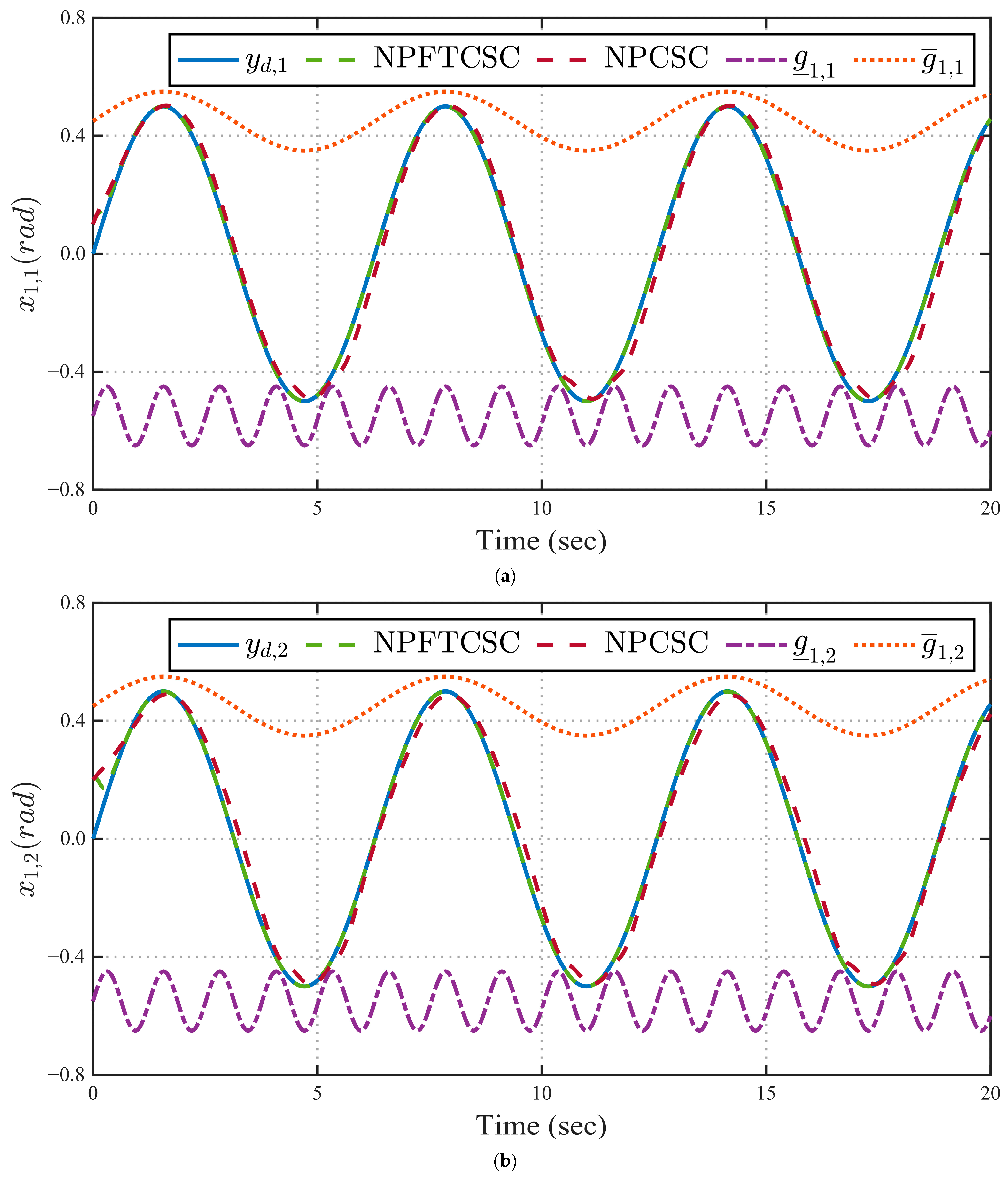
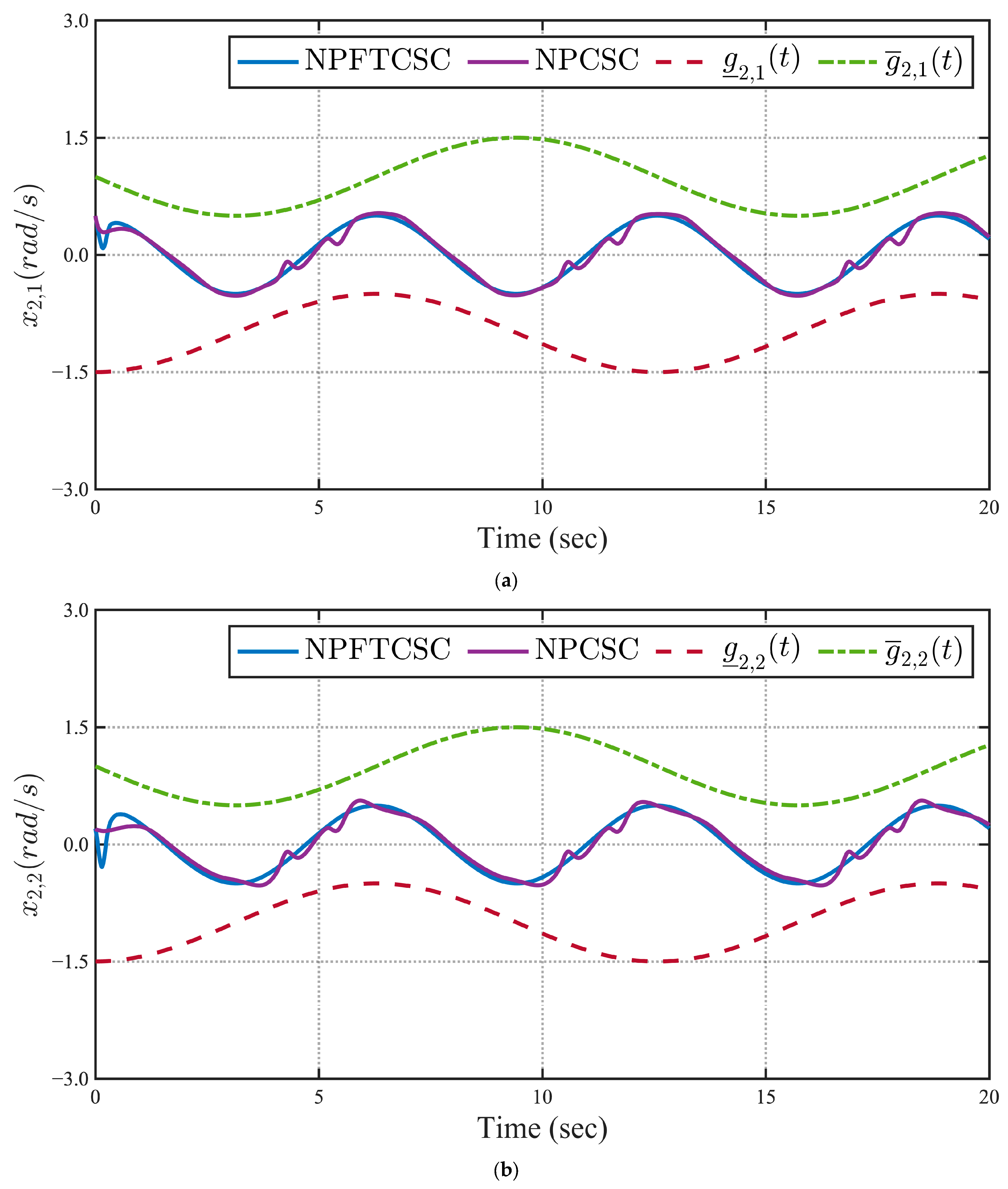
Theorem 1. 

Consider the dynamics of an $n$ DOF robotic manipulator (1) under Assumptions 1–3 and the conditions a, b, c, d, with the virtual control law (16), the update equations of RBFNNs weights (18) and the command filter (13)–(15). By appropriately setting the parameters $k_1$, $k_2$, $k_3$, $k_4$, $k_5$, $k_6$, $k_7$, $\omega$, $\gamma$ and $\eta$, if the initial value of tracking error satisfies ${\underset{\_}{g}}_e\left(0\right)<e_1\left(0\right)<{\bar{g}}_e\left(0\right)$, then the actual control law (17) ensures the state $x_1$ track the given reference trajectory $y_d$ with the given tracking quality, while guaranteeing no violation of constraints (3). The signals of the closed-loop system converge within a finite time $T$ . The settling time is

$$T≔max\left\{{\displaystyle \frac{\ln \left(\frac{\mathsf{\alpha }\rho V^{1-\frac{p+1}{2}}\left(0\right)+\beta }{\beta }\right)}{\mathsf{\alpha }\rho \left(1-\frac{p+1}{2}\right)}},{\displaystyle \frac{\ln \left(\frac{\mathsf{\alpha }{V}^{1-\frac{p+1}{2}}\left(0\right)+\rho \beta }{\rho \beta }\right)}{\mathsf{\alpha }\left(1-\frac{p+1}{2}\right)}}\right\}.$$

(19)

Proof. 

Selecting the candidate Lyapunov function $V={\displaystyle \frac{1}{2}}\left(v_1^T{v}_1+v_2^T{v}_2+{\tilde{D}}^T\tilde{D}+{\eta }^{-1}tr\left({\tilde{W}}^T\tilde{W}\right)\right)$ and differentiating it, one gets:

$$\begin{array}{c}\dot{V}=v_1^T\left({\mu }_e^1\left({\mu }_1^1\left(x_2-{\mu }_1^2\right)-{\dot{\epsilon }}_r-{\mu }_e^2\right)+v_2-{\epsilon }_2+a_d+{\zeta }_2-\dot{{\zeta }_1}\right)\\ +v_2^T\left({\mu }_2^1\left(M^{-1}\tau +W^T\varphi +D-{\mu }_2^2\right)-{\dot{a}}_d-\dot{{\zeta }_2}\right)\\ +{\tilde{D}}^T\dot{\tilde{D}}+{\eta }^{-1}tr\left({\tilde{W}}^T\dot{\tilde{W}}\right),\end{array}$$

(20)

where $\tilde{D}=D-\widehat{D}$; $\tilde{W}=W-\widehat{W}$. Substituting compensating signals (13), (14) the virtual control signal (16) and control law (17) into (20) yields:

$$\begin{array}{c}\dot{V}={-k}_2{‖v_1‖}^2{-k}_3{‖v_1‖}^{p+1}{-k}_4{‖v_2‖}^2{-k}_5{‖v_2‖}^{p+1}\\ +v_2^T{\mu }_2^1\left({\tilde{W}}^T\varphi +\tilde{D}\right)+{\tilde{D}}^T\dot{\tilde{D}}+{\eta }^{-1}tr\left({\tilde{W}}^T\dot{\tilde{W}}\right).\end{array}$$

(21)

Differentiating the first expression in (6) gives:

$$\dot{\tilde{D}}=-\gamma \tilde{D}-\gamma {\tilde{W}}^T\varphi +k_1{\widehat{D}}^p+\dot{D}.$$

(22)

where $\dot{D}={\displaystyle \frac{\partial \delta }{\partial Z}}\dot{Z}-M^{-1}\dot{M}{M}^{-1}d+M^{-1}\dot{d}$. The inertia matrix $M^{-1}$ is always bounded [3,4]. Recalling Equations (2) and (4), $\delta { = M}^{-1}\left(-{Cx}_2-G\right)-W^T\varphi \left(Z\right)$ ensures that ${\displaystyle \frac{\partial \delta }{\partial Z}}$ is bounded. The boundedness of $\dot{Z}$ depends on $\tau$. Utilizing proof by contradiction, it is assumed that $\tau$ is unbounded. Since $x_2$ is continuously differentiable ($\tau$ is a continuous function), $x_2$ is also unbounded. Therefore, the unbounded control signal cannot guarantee the boundedness of $x_2$. If there exists a control law $\tau$ such that $x_2$ is bounded, then $\tau$ must be bounded. From Assumption 2, it can be known that $d$ and $\dot{d}$ are also bounded. Therefore, $\dot{D}$ is bounded and its supremum of the second norm denoted as $‖\dot{D}‖\le M_1$, $M_1$ is a positive constant. Substituting (18), (22) into (21) yields:

$$\begin{array}{c}\begin{array}{c}\dot{V}={-k}_2{‖v_1‖}^2{-k}_3{‖v_1‖}^{p+1}{-k}_4{‖v_2‖}^2{-k}_5{‖v_2‖}^{p+1}\\ +v_2^{\mathrm{T}}{\mu }_2^1\tilde{D}-\gamma {‖\tilde{D}‖}^2-\gamma {\tilde{D}}^T{\tilde{W}}^T\varphi +k_1{\tilde{D}}^T{\widehat{D}}^p+{\tilde{D}}^T\dot{D}\end{array}\\ +\mathrm{t}\mathrm{r}\left(k_6{\tilde{W}}^{\mathrm{T}}\widehat{W}+k_7{\tilde{W}}^{\mathrm{T}}{\widehat{W}}^{\left(p\right)}\right).\end{array}$$

(23)

Here ${\widehat{W}}^{\left(p\right)}=\left[\begin{array}{ccc}{\widehat{w}}_1^p& \dots & 0_{l\times 1}\\ ⋮& \ddots & ⋮\\ 0_{l\times 1}& \dots & {\widehat{w}}_n^p\end{array}\right]$. Utilizing Young’s inequality to decouple $v_2^{\mathrm{T}}{\mu }_2^1\tilde{D}$, $-\gamma {\tilde{D}}^T{\tilde{W}}^T\varphi$, ${\tilde{D}}^T\dot{D}$ and $k_6{\tilde{W}}^{\mathrm{T}}\widehat{W}$, one gets:

$$\left\{\begin{array}{c}{v}_2^{\mathrm{T}}{\mu }_2^1\tilde{D}\le {\displaystyle \frac{\overline{\mathrm{s}}}{2}}{‖v_2‖}^2+{\displaystyle \frac{\overline{\mathrm{s}}}{2}}{‖\tilde{D}‖}^2,\\ -\gamma {\tilde{D}}^T{\tilde{W}}^T\varphi \le {\displaystyle \frac{\gamma nl}{2}}{‖\tilde{W}‖}_F^2+{\displaystyle \frac{\gamma }{2}}{‖\tilde{D}‖}^2,\\ {\tilde{D}}^T\dot{D}\le {\displaystyle \frac{1}{2}}{‖\tilde{D}‖}^2+{\displaystyle \frac{1}{2}}{M}_1^2,\\ k_6{\tilde{W}}^{\mathrm{T}}\widehat{W}\le -{\displaystyle \frac{k_6}{2}}{‖\tilde{W}‖}_F^2+{\displaystyle \frac{k_6}{2}}{‖W‖}_F^2.\end{array}\right.$$

(24)

Note that ${\tilde{D}}_i^{1+p}$=${\left|\tilde{D}\right|}_i^{1+p}$. According to Lemma 1, the following inequality holds:

$$\left\{\begin{array}{c}{k}_1{\tilde{D}}^T{\widehat{D}}^p\le -k_1{l}_1{‖\tilde{D}‖}^{1+p}+k_1{l}_2{\underset{\_}{1}}^T{D}^{1+p},\\ k_{7}tr\left({\tilde{W}}^{\mathrm{T}}{\widehat{W}}^{\left(p\right)}\right)\le -k_7{l}_1{tr\left({\tilde{W}}^{\mathrm{T}}\tilde{W}\right)}^{{\displaystyle \frac{1+p}{2}}}+k_7{l}_2{\displaystyle \sum _{i=1}^n}{\underset{\_}{1}}^T{w}_i^{1+p},\end{array}\right.$$

(25)

where $\underset{\_}{1}={\left[1,\dots ,1\right]}^T\in {\mathbb{R}}^n$. Substituting (24), (25) into (23), yields:

$$\begin{array}{c}\begin{array}{c}\dot{V}\le {-k}_2{‖v_1‖}^2{-k}_3{‖v_1‖}^{p+1}{-\left(k_4-{\displaystyle \frac{\overline{s}}{2}}\right)‖v_2‖}^2{-k}_5{‖v_2‖}^{p+1}\\ -\left({\displaystyle \frac{\gamma }{2}}-{\displaystyle \frac{\overline{s}}{2}}-{\displaystyle \frac{1}{2}}\right){‖\tilde{D}‖}^2-k_1{l}_1{‖\tilde{D}‖}^{1+p}-{\displaystyle \frac{k_6}{2}}{‖\tilde{W}‖}_F^2-k_7{l}_1{tr\left({\tilde{W}}^{\mathrm{T}}\tilde{W}\right)}^{{\displaystyle \frac{1+p}{2}}}\end{array}\\ {\displaystyle \frac{1}{2}}{M}_1^2+{\displaystyle \frac{k_6}{2}}{W}_M^2+k_1{l}_2{\underset{\_}{1}}^T{D}^{1+p}+k_7{l}_2{\displaystyle \sum _{i=1}^n}{\underset{\_}{1}}^T{w}_i^{1+p}.\end{array},$$

(26)

Recalling the definition of $V$ and applying in [[37], Lemmas 3.3 and 3.4], from (26) one can obtain

$$\begin{array}{c}\dot{V}\le -2\beta \left(v_1^T{v}_1+v_2^T{v}_2+{\tilde{D}}^T\tilde{D}+{\eta }^{-1}tr\left({\tilde{W}}^T\tilde{W}\right)\right)\\ -2\mathsf{\alpha }{\left(v_1^T{v}_1+v_2^T{v}_2+{\tilde{D}}^T\tilde{D}+{\eta }^{-1}tr\left({\tilde{W}}^T\tilde{W}\right)\right)}^{{\displaystyle \frac{p+1}{2}}}+\mathsf{\Delta },\end{array}$$

(27)

where $\Delta ={\displaystyle \frac{1}{2}}{M}_1^2+{\displaystyle \frac{k_6}{2}}{W}_M^2+k_1{l}_2{\underset{\_}{1}}^T{D}^{1+p}+k_7{l}_2\sum _{i=1}^n{\underset{\_}{1}}^T{w}_i^{1+p}$

$\beta =\min \left(k_2,k_4-{\displaystyle \frac{\overline{\mathrm{s}}}{2}},{\displaystyle \frac{\gamma }{2}}-{\displaystyle \frac{\overline{\mathrm{s}}}{2}}-{\displaystyle \frac{1}{2}},{\displaystyle \frac{k_6}{2}}\right)$,

$\mathsf{\alpha }=\mathrm{m}\mathrm{i}\mathrm{n}(k_3,k_5,{k_{1}l}_1,k_7{l}_1)$.

Following the definition of $V$ and (27), we can know that the signals $v_1$, $v_2$, $\tilde{D}$ and $\tilde{W}$ are bounded. Since $\tilde{D}=D-\widehat{D}$; $\tilde{W}=W-\widehat{W}$ and the fact that $W$ is constant and $D$ is bounded from Assumption 2 and the RBFNNs approximation property, the signals $\widehat{D}$ and $\widehat{W}$ are bounded. The boundedness of the filter output $a_d$ and the compensating signals ${\zeta }_k$ have been well discussed in [22]. They are also bounded. From (9)–(12), ${\epsilon }_1$, ${\epsilon }_2$ and ${\epsilon }_{\mathrm{e}}$ are bounded. Through (6) and (7), we know that $\dot{\widehat{W}}$ and $\dot{\widehat{D}}$ are bounded. All signals of the closed-loop system reach a compact set defined by $V$ in a finite time. The settling time expression (19) follows directly from Lemma 2. The boundedness of ${\epsilon }_{\mathrm{e}}$ ensures the given tracking performance. The boundedness of ${\epsilon }_1$ and ${\epsilon }_2$ ensures that the constraints of $x_1$ and $x_2$ are not violated. This completes the proof of Theorem 1. □

Remark 9. 

By the definition of $V$ and (27) we can conclude for $\forall t\ge T$, the tracking error  $e_1$  converges to the bounded set  ${\Omega }_{{\epsilon }_{e1}}^{\prime }=\left\{V\left(\left[e_1,{\underset{\_}{g}}_e{,\bar{g}}_e,{\zeta }_1,v_2,\tilde{D},\tilde{W}\right]\right)\le {\displaystyle \frac{\Delta }{2\beta }}\right\}$. Further for  $\forall t\ge 0$,  $x_k\in {\Omega }_{{\epsilon }_{k1}}=\left\{V\left(\left[v_1,v_2,\tilde{D},\tilde{W}\right]\right)\le {\displaystyle \frac{\Delta }{2\beta }}\right\}\bigcup \left\{‖x_k‖\le arc\left\{V\left(0\right)\right\}\right\}$, where  $arc\left\{\cdot \right\}$  is the inverse function of the function in parentheses.

Remark 10. 

The constraint of $e_1$ can be define as ${\underset{\_}{g}}_{e,i}=\left({\underset{\_}{g}}_{0,i}-{\underset{\_}{g}}_{\infty ,i}\right)e^{-{\kappa }_{i}t}+{\underset{\_}{g}}_{\infty ,i}$ and ${\bar{g}}_{e,i}=\left({\overline{g}}_{0,i}-{\overline{g}}_{\infty ,i}\right)e^{-{\kappa }_{i}t}+{\overline{g}}_{\infty ,i}$ . The initial value of ${\underset{\_}{g}}_{e,i}$ and ${\bar{g}}_{e,i}$ (i.e., ${\underset{\_}{g}}_{0,i}$ and ${\overline{g}}_{0,i}$ ) can be designed to be large enough so that $e_{1,i}\left(0\right)$ is within the constraint. The transient performance of the tracking error $e_1$ can be guaranteed by ${\kappa }_i$ and the steady-state error by ${\underset{\_}{g}}_{\infty ,i}$ and ${\overline{g}}_{\infty ,i}$ . the steady-state error $\left|e_{1,i}\right|\le {\overline{g}}_{\infty ,i}-{\underset{\_}{g}}_{\infty ,i}$.

Remark 11. 

It is well known that a system with a command filter can be divided into a fast subsystem and a rigid subsystem. According to singular perturbation theory, filter (15) is a boundary layer. If $\omega$ is small enough, the boundary layer equation is reduced and $a$ is approximately equal to $a_d$ . Or more precisely in [21,22] there exists a small enough ${\omega }_0>0$ such that $\left|a-a_d\right|\le \chi$, $\chi >0$ is positive constant. Therefore, $\omega$ should at least be designed to be less than the system’s bandwidth, such that the output of the filter can track the virtual control law with sufficient accuracy.

Remark 12. 

By Inequality (27) $k_2,k_4,\gamma , k_6$ determine the range of final convergence. $\Delta$ is a constant. The larger $k_2,k_4$ are, the larger $\beta$ is, and the smaller ${\displaystyle \frac{\Delta }{2\beta }}$ is. In addition, if ${\epsilon }_e\to 0$ then $e_{1,i}\to {\displaystyle \frac{{\overline{g}}_{\infty ,i}+{\underset{\_}{g}}_{\infty ,i}}{2}}$ . For details, see [36]. Let ${\displaystyle \frac{{\overline{g}}_{\infty ,i}+{\underset{\_}{g}}_{\infty ,i}}{2}}=0$, then increasing $k_2,k_4$ is beneficial to improving steady-state tracking accuracy.

Remark 13. 

When the value of $V$ is large enough, the fractional term in (27) takes a dominant position. Therefore, the larger $k_3,k_5,k_1,k_7$ are, the larger $\alpha$ is, and the smaller the decay time is.

4. Simulations

In order to verify the effectiveness and benefits of the proposed control scheme, comparisons are made between NP-based control with state constraints (NPCSC) [23,24,25,26,27] and the proposed NP-based finite-time control with state constraints (NPFTCSC) in this paper. The geometric and inertial parameters are adopted from [38].

$$\begin{array}{c}M(q)=\left[\begin{array}{cc}{p}_1+p_2+2p_3\cos q_2& p_2+p_3\cos q_2\\ p_2+p_3\cos q_2& p_2\end{array}\right],\\ C(q,\dot{q})=\left[\begin{array}{cc}-p_3{\dot{q}}_2\mathrm{c}\mathrm{o}\mathrm{s}& q_2-p_3\left({\dot{q}}_1+{\dot{q}}_2\right)\mathrm{s}\mathrm{i}\mathrm{n} q_2\\ p_3{\dot{q}}_2\mathrm{c}\mathrm{o}\mathrm{s} q_2& 0\end{array}\right],\\ G(q)=\left[\begin{array}{c}{p}_{4}g\cos q_1+p_{5}g\cos \left(q_1+q_2\right)\\ p_{5}g\cos \left(q_1+q_2\right)\end{array}\right].\end{array}$$

where $p_1=m_1{l}_{c1}^2+m_2{l}_1^2+I_1, p_2=m_2{l}_{c2}^2+I_2, p_3=m_2{l}_1{l}_{c2}, p_4=m_1{l}_{c2}+m_2{l}_{c2}$, $p_5=m_2{l}_{c2}, I_i$ is the inertia of the $i$-th rod, $I_1={\displaystyle \frac{1}{4}}{m}_1{l}_1^2$, $I_2={\displaystyle \frac{1}{4}}{m}_2{l}_2^2$. Their parameters are: $m_1=2.3 \mathrm{k}\mathrm{g},{ m}_2=0.8 \mathrm{k}\mathrm{g},{ l}_1=1 \mathrm{m}, l_2=1 \mathrm{m}$. The initial position and velocity are $q_1\left(0\right)=0.2$, $q_2\left(0\right)=0.1, {\dot{q}}_1\left(0\right)=0.4$ and ${\dot{q}}_2\left(0\right)=0.5.$ The desired trajectory is $y_d=[0.5\mathrm{s}\mathrm{i}\mathrm{n} (t),0.5\mathrm{s}\mathrm{i}\mathrm{n} (t\left)\right], t\in \left[\mathrm{0,20}\right]$. The external disturbances are: $d=[0.5\ast \mathrm{s}\mathrm{i}\mathrm{n} (t)+0.7\ast \mathrm{c}\mathrm{o}\mathrm{s} (t);0.5\ast \mathrm{c}\mathrm{o}\mathrm{s} (t)+0.4\ast \mathrm{s}\mathrm{i}\mathrm{n} (t\left)\right], t\in [0,20].$ The controller parameters are configured as $k_1=0.1$, $k_2=5$, $k_3=5$, $k_4=2$, $k_5=2$, $k_6=2$, $k_5=1$, $\omega =0.01$, $\gamma =10$, $p={\displaystyle \frac{3}{5}}$, $\eta =10$. The coordinate transformations are chosen as ${\mathsf{\Phi }}_k\left({\epsilon }_k\left(t\right),t\right)={\displaystyle \frac{{\bar{g}}_{k,i}\left(t\right)e^{{\epsilon }_k}+{\underset{\_}{g}}_{k,i}\left(t\right)}{e^{{\epsilon }_k}+1}}.$ The predefine constraints are chosen as ${\bar{g}}_{\mathrm{1,1}}={\bar{g}}_{\mathrm{1,2}}=0.45+0.1\mathrm{s}\mathrm{i}\mathrm{n}\left(\mathrm{t}\right),$ ${\underset{\_}{g}}_{\mathrm{1,1}}={\underset{\_}{g}}_{\mathrm{1,2}}=-0.55+0.1\mathrm{s}\mathrm{i}\mathrm{n} \left(5\mathrm{t}\right)$, ${\bar{g}}_{\mathrm{2,1}}={\bar{g}}_{\mathrm{2,2}}=1-0.5\mathrm{s}\mathrm{i}\mathrm{n} \left(0.5\mathrm{t}\right),$ ${\underset{\_}{g}}_{\mathrm{2,1}}={\underset{\_}{g}}_{\mathrm{2,2}}=-1+0.5\mathrm{c}\mathrm{o}\mathrm{s} \left(0.5\mathrm{t}\right)$. ${\underset{\_}{g}}_{e,i}=\left(-2.5+0.1\right)e^{-5t}-0.1$, ${\bar{g}}_{\mathrm{e},i}=\left(2.5-0.1\right)e^{-5t}+0.1$.

Like [39], the quantitative evaluation of the proposed control was assessed using integral absolute error (IAE), integral of squared error (ISE) and control energy (CE), with the calculated results presented in

Table 2. Quantitative evaluation of the controllers NPCSC and NPFTCSC.

	Performance Evaluation Metrics	IAE	ISE	CE
Control Scheme
NPCSC		1.571 $\mathrm{r}\mathrm{a}\mathrm{d}\cdot \mathrm{s}$	0.107 ${\mathrm{r}\mathrm{a}\mathrm{d}}^2\cdot \mathrm{s}$	6.107
NPFTCSC		0.368 $\mathrm{r}\mathrm{a}\mathrm{d}\cdot \mathrm{s}$	0.056 ${\mathrm{r}\mathrm{a}\mathrm{d}}^2\cdot \mathrm{s}$	6.348

.$\mathrm{CE} =\sum _{i=1}^N{\displaystyle \frac{1}{{\tau }_{\mathrm{rated},\mathrm{i} }^2\cdot T_s}}\int {\tau }_i^{2}dt$. Simulation time $T_s=20$; Rated output torque ${\tau }_{\mathrm{rated},1}=20\left(\mathrm{N}\mathrm{m}\right), {\tau }_{\mathrm{rated},2}=5\left(\mathrm{N}\mathrm{m}\right)$. ISE = $\int {‖e_1‖}^{2}dt$, IAE = $\sum _{i=1}^N\int \left|e_{1,i}\right|dt$.

It is seen from Figure 3 and Figure 4 that under the proposed control algorithm (17) with adaptive law (18) and DOB (6), as long as the initial values of states satisfy Assumption 1 and appropriate tracking-error constraints are chosen, the full-state constraints are not violated for $t\ge 0$. The responses of actual tracking errors $E_{\mathrm{1,1}}$ and $E_{\mathrm{1,2}}$ are shown in Figure 5, which are always bounded. Figure 6 demonstrates that under the controller (16), the compensation errors achieve finite-time convergence, which guarantees rapid convergence of ${\epsilon }_e$ into a bounded set. The tracking errors can be regulated by the prescribed constraints ${\underset{\_}{g}}_{e,k}$ and ${\bar{g}}_{e,k}$ as illustrated in Figure 7. These constraints simultaneously guarantee both transient and steady-state performance of tracking errors. Compared with NPCSC, the proposed algorithm achieves faster convergence rates and smaller overshoot magnitudes, as evidenced in Figure 5. From Figure 3 it is seen that NPCSC fails to maintain satisfactory tracking performance near constraint boundaries (e.g., at $t\approx 5 \mathrm{s}, 10 \mathrm{s},$ and $17 \mathrm{s}$). The controller conservatively prioritizes constraint satisfaction over tracking accuracy, resuming signal tracking only when distant from constraints. This behavior thereby leads to torque oscillations as shown in Figure 8. Crucially, the reference trajectory $y_d$ satisfies the constraints ${\underset{\_}{g}}_{1,i}$ and ${\bar{g}}_{1,i}$ at all times. Any constraint violation can solely originate from system uncertainties. Therefore, the proposed algorithm enhances tracking precision relative to NPCSC, it retains certain conservatism regarding constraint handling. The accelerated convergence entails higher energy consumption during initial operation, quantified in Table 2. The proposed method retains the core advantage of NPCSC over conventional BLF/IBLF-based approaches: the virtual control law inherently bypasses feasibility conditions. This property has been comprehensively demonstrated in [23] and thus will not be reiterated herein.

5. Conclusions

This paper proposes a novel control algorithm for robotic manipulators that guarantees finite-time tracking despite external disturbances and unknown system parameters, while ensuring preset constraint satisfaction and tracking performance. The DOB is designed to compensate for aggregate system uncertainties comprising unknown nonlinearities and disturbances. The proposed control scheme is designed based on nonlinear transformations not only achieves finite-time convergence, but also strictly guarantees full-state constraints while delivering prescribed tracking performance. Simulation results demonstrate the effectiveness and benefits of the proposed control scheme.

References

1. Qi, R.; Lam, H.-K.; Liu, J.; Yu, J. Adaptive Fuzzy Finite-Time Singular Perturbation Control for Flexible Joint Manipulators with State Constraints. IEEE Trans. Syst. Man Cybern. Syst. 2024, 54, 7521–7527. [Google Scholar] [CrossRef]
2. Spong, M.W.; Hutchinson, S.; Vidyasagar, M. Robot Modeling and Control; Wiley: New York, NY, USA, 2006. [Google Scholar]
3. Liu, Q.; Zhang, Z.; Li, J.; Bu, X.; Hanajima, N. Adaptive Neural Network Iterative Learning Control of Long-Stroke Hybrid Robots with Initial Errors and Full State Constraints. Meas. Control 2024, 58, 128–144. [Google Scholar] [CrossRef]
4. Lu, S.M.; Li, D.P.; Liu, Y.J. Adaptive Neural Network Control for Uncertain Time-Varying State Constrained Robotics Systems. IEEE Trans. Syst. Man Cybern. Syst. 2017, 49, 2511–2518. [Google Scholar] [CrossRef]
5. Luo, X.; Mu, D.; Wang, Z.; Ning, P.; Hua, C. Adaptive Full-State Constrained Tracking Control for Mobile Robotic System with Unknown Dead-Zone Input. Neurocomputing 2023, 524, 31–42. [Google Scholar] [CrossRef]
6. Zhao, K.; Song, Y.D.; Shen, Z.X. Neuroadaptive Fault-Tolerant Control of Nonlinear Systems under Output Constraints and Actuation Faults. IEEE Trans. Neural Netw. Learn. Syst. 2016, 29, 286–298. [Google Scholar] [CrossRef] [PubMed]
7. Zhao, K.; Song, Y.D.; Ma, T.; He, L. Prescribed Performance Control of Uncertain Euler–Lagrange Systems Subject to Full-State Constraints. IEEE Trans. Neural Netw. Learn. Syst. 2018, 29, 3478–3489. [Google Scholar] [PubMed]
8. Mayne, D.Q.; Rawlings, J.B.; Rao, C.V.; Scokaert, P.O.M. Constrained Model Predictive Control: Stability and Optimality. Automatica 2000, 36, 789–814. [Google Scholar] [CrossRef]
9. Bemporad, A. Reference Governor for Constrained Nonlinear Systems. IEEE Trans. Autom. Control 1998, 43, 415–419. [Google Scholar] [CrossRef]
10. Dehaan, D.; Guay, M. Extremum-Seeking Control of State-Constrained Nonlinear Systems. Automatica 2005, 41, 1567–1574. [Google Scholar] [CrossRef]
11. He, W.; Chen, Y.; Yin, Z. Adaptive Neural Network Control of an Uncertain Robot with Full-State Constraints. IEEE Trans. Cybern. 2016, 46, 620–629. [Google Scholar] [CrossRef] [PubMed]
12. Li, C.; Zhao, L.; Xu, Z. Finite-Time Adaptive Event-Triggered Control for Robot Manipulators with Output Constraints. IEEE Trans. Circuits Syst. II Express Briefs 2022, 69, 3824–3828. [Google Scholar] [CrossRef]
13. Fang, X.; Fan, H.; Liu, L.; Wang, B. Adaptive Fixed-Time Fault-Tolerant Control of Saturated MIMO Nonlinear Systems with Time-Varying State Constraints. Nonlinear Dyn. 2022, 110, 3463–3483. [Google Scholar] [CrossRef]
14. Zhang, J.; Yan, C.; Xia, J.; Shen, H.; Xie, X. Dynamic Event-Triggered-Based Adaptive Fuzzy Optimized Control for Slowly Switched Nonlinear System with Intermittent State Constraints. Inf. Sci. 2024, 674, 120717. [Google Scholar] [CrossRef]
15. Li, D.P.; Liu, Y.J.; Tong, S.; Chen, C. Neural Networks-Based Adaptive Control for Nonlinear State Constrained Systems with Input Delay. IEEE Trans. Cybern. 2018, 49, 1249–1258. [Google Scholar] [CrossRef] [PubMed]
16. Wu, Y.; Xie, X.-J. Robust Adaptive Control for State-Constrained Nonlinear Systems with Input Saturation and Unknown Control Direction. IEEE Trans. Syst. Man Cybern. Syst. 2021, 51, 1192–1202. [Google Scholar] [CrossRef]
17. Cui, B.; Xia, Y.; Liu, K.; Shen, G. Finite-Time Tracking Control for a Class of Uncertain Strict-Feedback Nonlinear Systems with State Constraints: A Smooth Control Approach. IEEE Trans. Neural Netw. Learn. Syst. 2020, 31, 4920–4932. [Google Scholar] [CrossRef] [PubMed]
18. Sun, W.; Su, S.F.; Wu, Y.Q.; Xia, J.W.; Nguyen, V.T. Adaptive Fuzzy Control with High-Order Barrier Lyapunov Functions for High-Order Uncertain Nonlinear Systems with Full-State Constraints. IEEE Trans. Cybern. 2020, 50, 3424–3432. [Google Scholar] [CrossRef] [PubMed]
19. Phan, V.D.; Truong, H.; Le, V.C.; Ho, S.P.; Ahn, K.K. Adaptive Neural Observer-Based Output Feedback Anti-Actuator Fault Control of a Non-Linear Electro-Hydraulic System with Full State Constraints. Sci. Rep. 2025, 15, 3044. [Google Scholar] [CrossRef] [PubMed]
20. Pan, C.; Huang, H.; Chen, C.; Wu, L.; Xiao, J. Neuro-Adaptive Command-Filtered Backstepping Control of Uncertain Flexible-Joint Manipulators with Input Saturation via Output. Sci. Rep. 2025, 15, 17254. [Google Scholar] [CrossRef] [PubMed]
21. Sui, S.; Chen, C.L.P.; Tong, S. Command Filter-Based Predefined Time Adaptive Control for Nonlinear Systems. IEEE Trans. Autom. Control 2024, 69, 7863–7870. [Google Scholar] [CrossRef]
22. Farrell, J.A.; Polycarpou, M.; Sharma, M.; Dong, W. Command Filtered Backstepping. IEEE Trans. Autom. Control 2009, 54, 1391–1395. [Google Scholar] [CrossRef]
23. Zhao, K.; Song, Y. Neuroadaptive Robotic Control under Time-Varying Asymmetric Motion Constraints: A Feasibility-Condition-Free Approach. IEEE Trans. Cybern. 2018, 50, 15–24. [Google Scholar] [CrossRef] [PubMed]
24. Ji, Q.; Chen, G.; He, Q. Neural Network-Based Distributed Finite-Time Tracking Control of Uncertain Multi-Agent Systems with Full State Constraints. IEEE Access 2020, 8, 174365–174374. [Google Scholar] [CrossRef]
25. Zhang, T.; Xia, M.; Yi, Y.; Shen, Q. Adaptive Neural Dynamic Surface Control of Pure-Feedback Nonlinear Systems with Full State Constraints and Dynamic Uncertainties. IEEE Trans. Syst. Man Cybern. Syst. 2017, 47, 2378–2387. [Google Scholar] [CrossRef]
26. Guo, T.; Wu, X. Backstepping Control for Output-Constrained Nonlinear Systems Based on Nonlinear Mapping. Neural Comput. Appl. 2014, 25, 1665–1674. [Google Scholar] [CrossRef]
27. Ning, P.; Mu, D.; Hua, C. Global Prescribed-Time Tracking Control Mobile Robot Systems with Performance Constraints. IEEE Trans. Circuits Syst. II Express Briefs 2023, 71, 181–185. [Google Scholar]
28. Gao, J.; Tan, Z.; Li, L.; Jia, G.; Liu, P.X. A Novel Finite-Time Non-Singular Robust Control for Robotic Manipulators. Chaos Solitons Fractals 2025, 194, 116266. [Google Scholar] [CrossRef]
29. Dang, V.T.; Nguyen, X.B.; Tran, T.D.T.; Le, D.T.; Nguyen, T.L. Finite-Time Velocity Sensorless Integral Sliding Mode Control for Roll-to-Roll Systems under Matched Disturbances. ISA Trans. 2025. [Google Scholar] [CrossRef] [PubMed]
30. Wang, Y.; Song, Y.; Krstic, M.; Wen, C. Fault-tolerant finite time consensus for multiple uncertain nonlinear mechanical systems under single-way directed communication interactions and actuation failures. Automatica 2016, 63, 374–383. [Google Scholar] [CrossRef]
31. Yu, J.; Shi, P.; Zhao, L. Finite-Time Command Filtered Backstepping Control for a Class of Nonlinear Systems. Automatica 2018, 92, 173–180. [Google Scholar] [CrossRef]
32. Sanner, R.M.; Slotine, J.J.E. Gaussian Networks for Direct Adaptive Control. In Proceedings of the 1991 American Control Conference, Boston, MA, USA, 26–28 June 1991; IEEE: Boston, MA, USA, 1991; pp. 2153–2159. [Google Scholar]
33. Park, J.; Sandberg, I.W. Universal Approximation Using Radial-Basis-Function Networks. Neural Comput. 1991, 3, 246–257. [Google Scholar] [CrossRef] [PubMed]
34. Nikiforov, V.; Gerasimov, D. Adaptive Regulation; Springer International Publishing: Cham, Switzerland, 2022. [Google Scholar]
35. Furtat, I.; Gushchin, P. Nonlinear Feedback Control Providing Plant Output in Given Set. Int. J. Control 2022, 95, 1533–1542. [Google Scholar] [CrossRef]
36. Nguyen, B.H.; Furtat, I.B. Output Stabilization of Linear Systems in Given Set. Mathematics 2023, 11, 3542. [Google Scholar] [CrossRef]
37. Zuo, Z.; Tie, L. A New Class of Finite-Time Nonlinear Consensus Protocols for Multi-Agent Systems. Int. J. Control 2013, 87, 363–370. [Google Scholar] [CrossRef]
38. Lewis, F.L.; Liu, K.; Yesildirek, A. Neural Net Robot Controller with Guaranteed Tracking Performance. IEEE Trans. Neural Netw. 1995, 6, 703–715. [Google Scholar] [CrossRef] [PubMed]
39. Venkaiah, P.; Sarkar, B.K.; Chatterjee, A. Harris Hawks Optimization Tuned Exponential Reaching Law Based Integral SMC for Pitch Control of Linear Hydraulic Actuated Wind Turbines. Proc. Inst. Mech. Eng. Part C J. Mech. Eng. Sci. 2023, 238, 1855–1873. [Google Scholar] [CrossRef]
Figure 1. Two-link manipulator.
Mathematics 13 02336 g001
Figure 2. Schematic of the proposed control scheme.
Mathematics 13 02336 g002
Figure 3. Responses of x 1,1 and x 1,2 . (a) Trajectories of x 1,1 and desired signal y d , 1 subject to the constraint g _ 1,1 < x 1,1 < g 1,1 . (b) Trajectories of x 1,2 and desired signal y d , 2 subject to the constraint g _ 1,2 < x 1,2 < g 1,2 .
Mathematics 13 02336 g003
Figure 4. Responses of x 2,1 and x 2,2 . (a) Trajectories of x 2,1 subject to the constraint g _ 2,1 < x 2,1 < g 2,1 . (b) Trajectories of x 2,2 subject to the constraint g _ 2,2 < x 2,2 < g 2,2 .
Mathematics 13 02336 g004
Figure 5. Trajectories of actual tracking errors. (a) Actual tracking error E 1,1 . (b) Actual tracking error E 1,2 .
Mathematics 13 02336 g005
Figure 6. Trajectories of compensation errors. (a) Position compensation error norm v 1 . (b) Angular velocity compensation error norm v 2 .
Mathematics 13 02336 g006
Figure 7. Tracking errors with preset performance constraints. (a) Trajectories of tracking error e 1,1 and preset performance constraints g _ e , 1 and g e , 1 . (b) Trajectories of tracking error e 1,2 and preset performance constraints g _ e , 2 and g e , 2 .
Mathematics 13 02336 g007
Figure 8. Input torques. (a) Input torque τ 1 . (b) Input torque τ 2 .
Mathematics 13 02336 g008