Research on Industrial Process Fault Diagnosis Method Based on DMCA-BiGRUN

Abstract

With the rising automation and complexity level of industrial systems, the efficiency and accuracy of fault diagnosis have become a critical challenge. The convolutional neural network (CNN) has shown some success in the fault diagnosis field. However, typical convolutional kernels are commonly fixed-sized, which makes it difficult to capture multi-scale features simultaneously. Additionally, the use of numerous fixed-size convolutional filters often results in redundant parameters. During the feature extraction process, the CNN often struggles to take inter-channel dependencies and spatial location information into consideration. There are also limitations in extracting various time-scale features. To address these issues, a fault diagnosis method on the basis of a dual-path mixed convolutional attention-BiGRU network (DMCA-BiGRUN) is proposed for industrial processes. Firstly, a dual-path mixed CNN (DMCNN) is designed to capture features at multiple scales while effectively reducing the parameter count. Secondly, a coordinate attention mechanism (CAM) is designed to help the network to concentrate on main features more effectively during feature extraction by combining the channel relationship and position information. Finally, a bidirectional gated recurrent unit (BiGRU) is introduced to process sequences in both directions, which can effectively learn the long-range temporal dependencies of sequence data. To verify the fault diagnosis performance of the proposed method, simulation experiments are implemented on the Tennessee Eastman (TE) and Continuous Stirred Tank Reactor (CSTR) datasets. Some deep learning methods are compared in the experiments, and the results confirm the feasibility and superiority of DMCA-BiGRUN.

1. Introduction

With the deep integration of information technology and intelligent manufacturing technology, the chemical system has become more complex, which places higher requirements on the safety and reliability of chemical processes [1]. In response to these challenges, advanced monitoring technologies for chemical processes are essential for maintaining equipment safety and improving production efficiency. Since chemical processes are highly coupled and dynamic, even minor deviations can lead to serious safety incidents or economic losses. Thus, intelligent diagnostic techniques are becoming increasingly important, which can promptly detect abnormalities and accurately identify faults in large-scale industrial datasets [2].

In order to achieve effective monitoring of complex chemical processes, fault detection and diagnosis (FDD) techniques have become prevalent in industrial applications. FDD methods are usually categorized into signal-based, model-based, and data-driven methods [3]. Signal-based FDD methods aim to identify faults by analyzing the variation characteristics inherent in processing variable signals. Typical signal-based FDD methods include time-domain analysis, frequency-domain analysis (such as Fourier transform), and time-frequency analysis (such as wavelet transform). These methods generally do not rely on physical mechanism modeling of the process but instead utilize the intrinsic patterns of the signals and data-driven feature pattern recognition. Márquez-Vera et al. proposed an inverse fuzzy fault model for fault detection and isolation. In their approach, the signals are preprocessed using the wavelet transform to highlight faulty features, and least angle regression is applied for variable selection to reduce the amount of data to be processed. The method was validated in the TE process, demonstrating its superior fault detection performance [4]. Within model-based FDD approaches, faults are detected, isolated, and identified by constructing and analyzing mathematical models of the system. The core idea is to use the difference between the system model and actual operating data to infer the existence and type of faults. Common model-based FDD methods include state estimation and fault tree analysis (FTA). State estimation methods include estimating the system state via a particle filter (PF) or Kalman filter (KF). By modeling the system’s physical rules, control logic, or process dynamics, experts can effectively identify and localize faults in the absence of rich historical data. Sadhukhan et al. proposed an adaptive traceless KF-based model for fault diagnosis of three-tank systems [5]. Cao and Du used an improved PF method based on a modified beetle swarm tentacle search algorithm validated in a doubly-fed induction generator fault diagnosis application [6]. Zhang et al. used FTA to analyze the causes of detector failures in nuclear power plants [7]. Although model-based FDD methods are characterized by high interpretability and low dependence on samples, they require high system modeling accuracy and rely heavily on experts’ knowledge and experience. Additionally, model construction and subsequent maintenance typically require lots of labor and time, resulting in high overall costs. In modern production processes, this method has difficulty efficiently coping with the large amounts of data continuously generated in intelligent factories, which limits its practical application.

In contrast, driven by significant progress in sensor technology and data acquisition methods, a large quantity of real-time, multidimensional operational data accumulated in industrial processes has become more accessible. As a result, data-driven FDD methods have gradually become a hotspot for research and application [8]. Data-driven FDD methods rely on the statistical analysis and modeling of process operation data. Machine learning or deep learning is then employed to automatically extract features and uncover hidden patterns from historical or real-time data. Then, the mapping relationship between fault categories and data is constructed to realize automatic system state identification and accurate fault type identification. It primarily consists of statistical analysis methods, as well as shallow and deep learning methods. The statistical analysis methods include Partial Least Squares (PLS) [9], Principal Component Analysis (PCA) [10], Canonical Correlation Analysis (CCA) [11], and Independent Component Analysis (ICA) [12]. Li et al. combined PCA with Liang–Kleeman Information Flow (LKIF) to quantify the causal interactions between nodes by introducing information flow, which improves the diagnostic efficiency of the TE process [13]. Xiu and Miao proposed a novel robust sparse CCA method for fault detection in the TE process [14]. These methods are relatively simple to implement and computationally efficient. However, they usually rely on linear assumptions and are sensitive to the data distribution, which makes it challenging to effectively handle the nonlinear features and complex coupling relationships in real industrial operations, ultimately affecting the accuracy of fault identification. Shallow learning methods are k-Nearest Neighbors (KNN) [15], Random Forest (RF) [16], Support Vector Machine (SVM) [17], artificial neural network (ANN) [18], Naive Bayes (NB) [19], and so on. Ye and Wei proposed a method based on SVM and a modified particle swarm optimization algorithm, which improved the accuracy of gas turbine fault diagnosis [20]. Han et al. developed a KPCA-RF fault diagnosis method based on kernel PCA (KPCA) and RF to address the issues existing in mainstream fault diagnosis methods for the TE process [21]. These methods have good nonlinear modeling capabilities, a strong classification performance, and low data distribution requirements. However, they require manual feature engineering and lack automatic feature learning capabilities. Additionally, their ability to process high-dimensional and complex data is restricted.

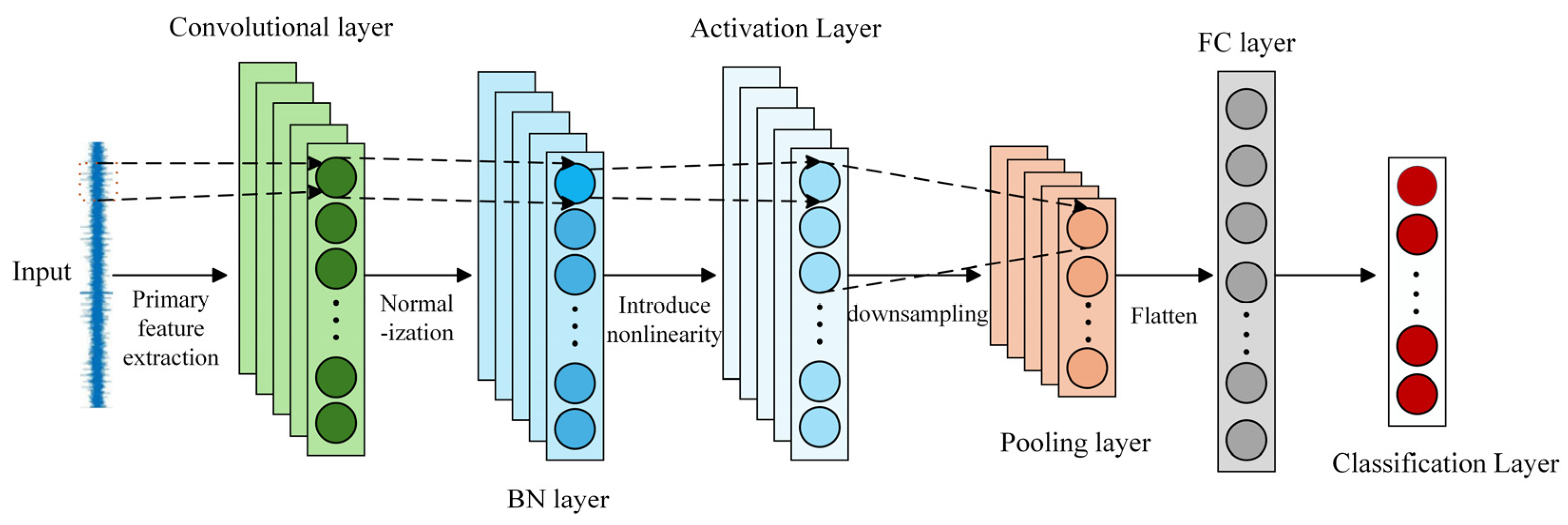
To overcome aforementioned problems, deep learning methods have been extensively studied in FDD tasks owing to their powerful ability to learn discriminative features. Some typical deep learning methods include the recurrent neural network (RNN) [22], Autoencoder (AE) [23], Deep Belief Network (DBN) [24], and CNN [25]. The CNN is one of the most common models, which can learn multi-level information representations from raw data automatically. It avoids a reliance on manual feature extraction and effectively improves fault recognition efficiency. The parameter sharing and sparse connection mechanisms not only achieve a significant reduction in parameter count and computational demands but also alleviate the overfitting problem and enhance the generalization capacity. The structure of the CNN is flexible and scalable. It can be embedded into other network structures or adjusted according to different tasks. Niu and Yang applied an improved one-dimensional CNN (1D-CNN) to the task of TE process fault diagnosis, which significantly improved diagnostic capability [26]. Xing et al. developed an optimized network structure based on 1D-CNN and its variant spatio-temporal CNN, introduced causal convolution to learn the historical information more efficiently, and applied it to fault diagnosis in chemical processes, which verified the superiority of the approach [27]. All these studies show the great potential of the CNN in fault diagnosis.

However, the CNN operates with a restricted perceptual scope due to its fixed-size convolution kernels, making it difficult to entirely grasp global contextual information from the raw data. To address this issue, researchers have proposed methods such as multi-scale convolution, dilated convolution, and attention mechanisms. Song and Jiang proposed a fault diagnosis approach for chemical processes by integrating a multi-scale CNN (MsCNN) with matrix graph representations, extracting multi-scale features through convolution kernels of different sizes [28]. Liang and Zhao designed a residual-enhanced one-dimensional dilated convolutional network, introducing a “zigzag” dilated convolution into the CNN, which effectively improves the receptive field of the convolutional layers [29]. Zhou et al. integrated a global attention mechanism with the convolutional architecture, which not only expands the receptive field but also dynamically adjusts the attention weights of different regions during feature extraction [30]. However, chemical processes are inherently dynamic systems, where process variables exhibit spatial coupling as well as significant temporal correlations, time delays, and dynamic evolution characteristics. Modeling based solely on static features is insufficient to fully capture system behavior. Therefore, recent research studies have increasingly focused on combining the local feature extraction capabilities of convolution with time-series modeling mechanisms. Through this combination, the dynamic features of process variables over time can be effectively captured, thus enhancing the robustness of FDD. Sun and Fan combined a long short-term memory (LSTM) network with a CNN, proposing a model incorporating a wide first-layer convolution and an LSTM network, which enables the joint learning of spatial and temporal features from process data [31]. Liang and Zhao proposed a multi-scale CNN integrated with bidirectional LSTM (BiLSTM) to capture multi-scale temporal information and correlated fault semantic features, which contributed to higher reliability in bearing fault diagnosis [32]. To improve the accuracy and efficiency of fault diagnosis under high-dimensional, nonlinear, and time-varying data, Zhang et al. proposed an enhanced deep CNN (EDCNN) model based on GRU, which effectively improved the fault diagnosis accuracy [33].

Although FDD methods based on deep learning have achieved relatively satisfactory outcomes, there are still several limitations. For instance, although convolutional structures enhance the feature extraction capability, they often come with a large number of parameters, which leads to high training costs [34]. Moreover, existing methods frequently overlook the integration of temporal dependencies and channel-wise information, making it difficult to fully capture the dynamic interactions among variables in complex industrial processes [35,36]. For example, although traditional LSTM-Fully Convolutional Network (LSTM-FCN) models combine temporal modeling and convolutional feature extraction, their convolutional parts often use single-scale fixed kernels, making it difficult to adapt to multi-scale faults. In addition, they lack attention mechanisms, resulting in limited recognition capability [37]. Models based on dilated convolutions, such as a temporal convolutional network (TCN), can capture long-term dependencies, but the causal convolution structure restricts the use of future information and lacks channel modeling, leading to weak sensitivity [38]. Multi-scale convolution models like MsCNN have a strong multi-scale feature extraction ability, but their complex structure and large number of parameters hinder deployment and generalization.

To overcome these difficulties, this paper proposes a novel network named the DMCA-BiGRUN, which integrates the DMCNN with the CAM and BiGRU, aiming to simultaneously take into account the high efficiency of spatial feature extraction, the selective attention ability of the CAM, and the temporal expression ability of sequence modeling.

In this paper, the main contributions are as follows:

(1)

A hybrid model integrating the DMCNN, CAM, and BiGRU is constructed for fault diagnosis in the industrial process. This model can realize multi-scale feature extraction, effectively overcoming the limitation of a CNN, which only extracts local features and suffers from redundant parameters. In addition, temporal dependencies among variables are captured, which enhances the identification of abnormal patterns in complex dynamic processes. This structure can achieve both efficient spatial feature extraction and the capture of temporal information, thereby improving the fault classification performance.

(2)

A CAM is proposed, which preserves global channel information and key features while incorporating positional information to reweight the original features. This enables the model to adaptively concentrate on critical feature information.

(3)

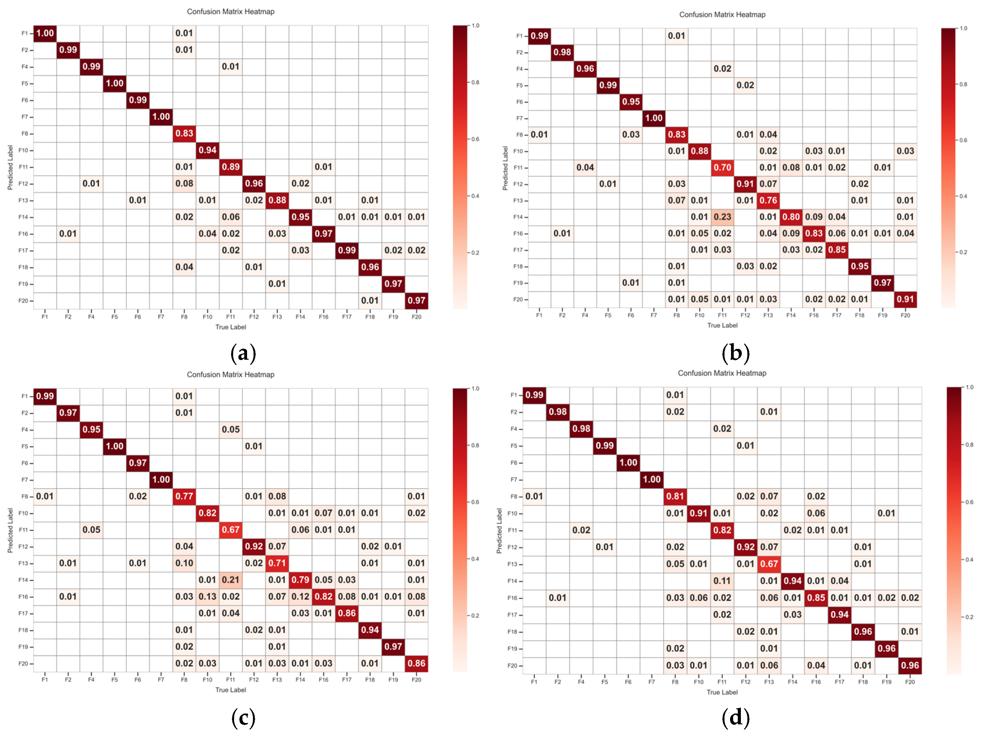
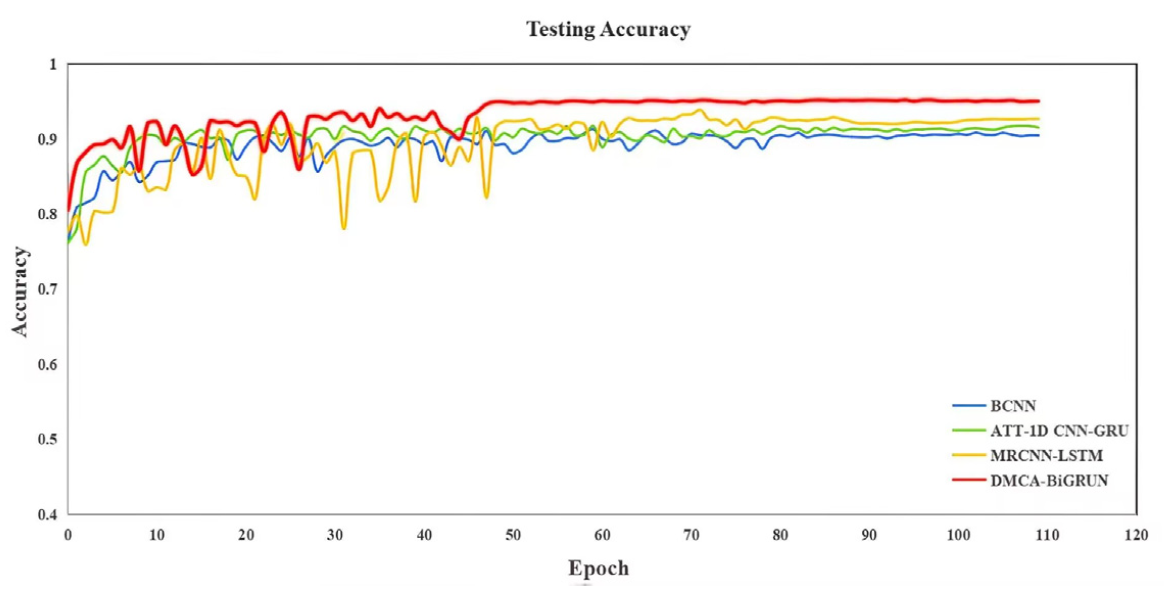
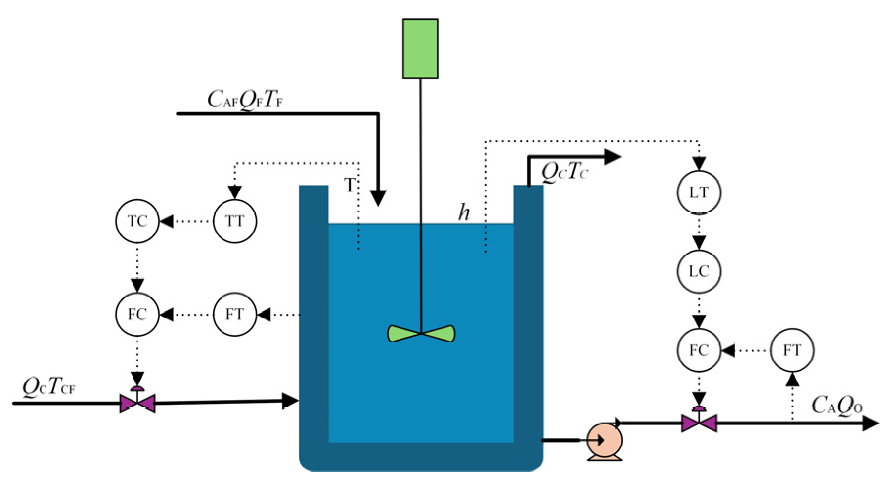
The proposed DMCA-BiGRUN is employed in the CSTR process and TE process to evaluate its performance. The experimental results demonstrate that the proposed method attains a 95.80% fault diagnostic accuracy in the TE process, which markedly outperforms the ablation and comparison models. In the CSTR process, the method also achieves an accuracy as high as 98.67%. These two sets of simulation experiments demonstrate the proposed method’s effectiveness and superiority in chemical processes’ fault diagnosis.

2. Preliminaries

2.1. Convolutional Neural Network

A CNN is a deep learning model that simulates the human visual system. It employs a local receptive field and a parameter-sharing mechanism to efficiently extract spatial features and automatically learn features without manual intervention. Because of its excellent feature learning and classification abilities, the CNN has been widely applied in industrial fault diagnosis. The CNN structure is demonstrated in Figure 1 [39].

The convolutional layer serves as the core component of the CNN. It possesses two key characteristics: a local receptive field and weight sharing, through which local features can be efficiently extracted and the number of parameters significantly reduced. Since this study deals with one-dimensional fault signals, a 1D-CNN is employed.

The Batch Normalization (BN) layer standardizes mini-batch data to reduce internal covariate shift, thereby accelerating training convergence and improving stability. Additionally, the noise introduced during normalization aids in preventing overfitting and improving the model’s generalization capability.

Since each layer of a neural network represents a linear transformation of the input, introducing nonlinear properties through an activation function allows the network model to handle complex, nonlinear features, thereby enhancing the model’s expressive capacity.

The pooling layer reduces computation and accelerates training through dimensionality reduction. The commonly used max pooling retains the most critical information in the feature map. The principle is shown in Figure 2.

2.2. MetaAconC Activation Function

The MetaAconC activation function determines whether to activate a neuron by dynamically adjusting the parameter λ_c, allowing the model to automatically concentrate on important channel features while adaptively suppressing unimportant ones. Its core idea is on-demand activation, which increases nonlinearity for important features while retaining near-linear behavior for less important ones. Thus, the model maintains its expressive power and avoids noise caused by excessive activation. The specific formula for the parameter λ_c is as follows:

$$\lambda c=\sigma (BN[H_4(BN[H_3({\displaystyle \frac{1}{L}}{\displaystyle \sum _{l=1}^L{x}_{(c,l)}})])])$$

(1)

First, the input feature x is averaged in the last dimension. Then, it is passed through two 1 × 1 convolution operations, H₃ and H₄, followed by a sigmoid function σ to obtain λ_c within the range of (0, 1). The parameter λ_c controls whether and to what extent the neuron is activated, where 0 indicates complete suppression of neuron activation. Finally, a set of learnable channel-level parameters e₁ and e₂ are established. Here, e₁ controls the degree of nonlinearity, and e₂ provides a linear baseline. Set e = e₁ − e₂. The result of the activation function, Y_Meta, is presented in Equation (2), where e₁ and e₂ can be adaptively adjusted through backpropagation [40].

$$Y_{Meta}=e\cdot x_{(c,l)}\cdot \sigma [\lambda c\cdot e\cdot x_{(c,l)}]+e_2\cdot x_{(c,l)}$$

(2)

The activation function avoids the neuron death problem caused by traditional activation functions and generates an independent adaptive parameter for each channel. This parameter controls two aspects: whether the neuron is activated and the degree of its activation.

2.3. Label Smooth Regularization

The standard cross-entropy loss function is optimized by forcing the model to push the predicted probability of the correct class to 1 and the other classes to 0. However, this may cause the model to be too extreme in the probability for the target class during prediction, leading to overfitting. Moreover, this approach is highly sensitive to noisy or incorrect labels since any mislabeled data can affect the model training. Therefore, a smoothing coefficient ε is added to soften the true label distribution and avoid overconfidence in the model. Label Smoothing Regularization (LSR) allows some of the probability distributions to be given to the other classes, which reduces the effect of noise. LSR not only improves the model’s generalization ability but also enhances its calibration performance.

In scenarios with imbalanced data, models often tend to overfit to the majority classes. LSR helps to suppress overfitting and reduces the model’s excessive reliance on majority classes, allowing it to focus on the majority classes while providing more opportunities to learn features of minority classes, thereby improving the recognition performance for underrepresented classes. In addition, by smoothing the label distribution, LSR reduces the loss function’s sensitivity to extreme prediction probabilities, making the gradient variation smoother. This contributes to more stable convergence when handling imbalanced data and helps alleviate the training difficulties caused by data imbalance. The computation process of the loss function after applying LSR, denoted as L_LSR, is as follows [41]:

$$\begin{array}{l}{L}_{\mathrm{LSR}}=-{\displaystyle \sum _{i=1}^C\tilde{y}(i})\log (p(i))\\ =-{\displaystyle \sum _{i=1}^C[(1-\epsilon )\cdot y(i)+\epsilon \cdot \frac{1}{C})]}\log (p(i))\\ =(1-\epsilon )[-{\displaystyle \sum _{i=1}^{C}y(i)}\log (p(i))]+\epsilon [{\displaystyle \frac{{\displaystyle {\sum }_{i=1}^C\log (p(i))}}{C}}]\\ =(1-\epsilon )L_{\mathrm{CE}}+\epsilon [{\displaystyle \frac{{\displaystyle {\sum }_{i=1}^C\log (p(i))}}{C}}]\end{array}$$

(3)

where p(i) is the predicted probability distribution of the model, y(i) is the original true labeling distribution, C represents the total number of categories, ỹ(i) corresponds to the true labeling distribution smoothed by the smoothing coefficient, and L_CE refers to the cross-entropy loss.

3. DMCA-BiGRUN

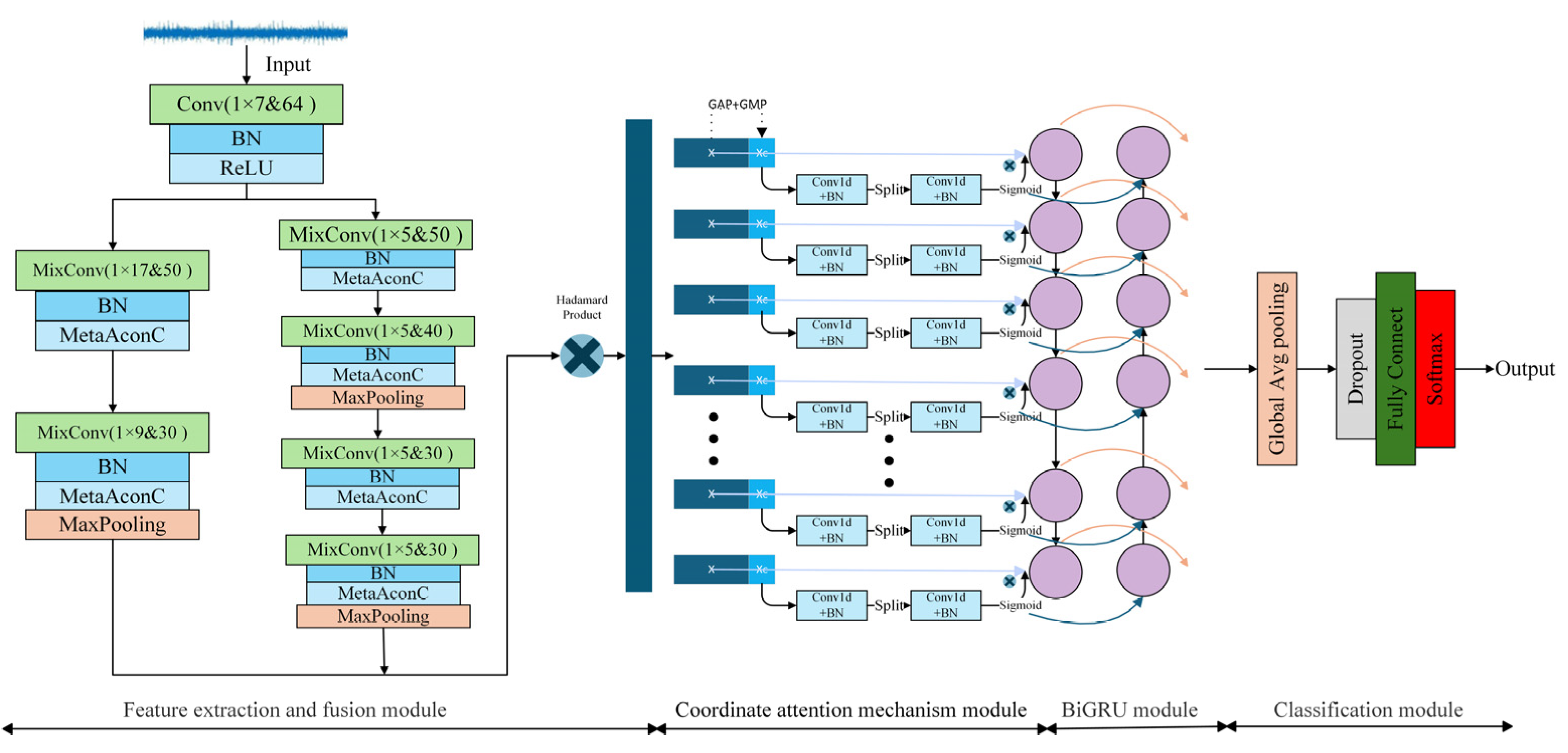
This paper proposes a model of a dual-path mixed convolutional attention-BiGRU network (DMCA-BiGRUN) for industrial fault diagnosis. It mainly consists of four modules: feature extraction module, coordinate attention mechanism module, BiGRU module, and classification module. Figure 3 displays the detailed architecture of the proposed DMCA-BiGRUN.

3.1. Feature Extraction and Fusion Module

This section proposes an improved CNN model, DMCNN, to address the challenges of multi-scale feature extraction and multi-variate coupling in fault diagnosis. DMCNN adopts dual-path convolution, using convolution kernels of different sizes to extract local details and global features, respectively. To reduce the parameters, each channel is individually processed through depthwise convolution, and residual connections are employed to supplement global information. Finally, pointwise convolution is used to fuse the channel features, and element-wise multiplication is applied to nonlinearly fuse the dual-path features. This helps the model learn complex relationships among variables while reducing the impact of noise.

The overall structure of the DMCNN is presented in Figure 4. First, the standardized data is fed into a standard convolutional layer with a kernel size of 1 × 7. The relatively large kernel helps filter out high-frequency noise and irrelevant features from the raw input during training. Low-level but global features of the faults are quickly extracted through a larger receptive field. The output from the standard convolutional layer is subsequently fed into a parallel dual-path mixed convolution network. The first path, referred to as the coarse-grained path, utilizes larger convolution kernels (1 × 17 and 1 × 9) to capture low-frequency, long-period signal features in industrial processes. It focuses on global information and long-term variation patterns. The kernel size is relatively reduced to avoid the problem of detail loss associated with a single oversized kernel. The choice of these larger kernels was guided by the fact that certain faults, such as those in the TE or CSTR processes, tend to develop gradually and require a sufficiently large receptive field for effective modeling. The second path is a fine-grained path designed to extract local and high-frequency features that typically occur over short time scales. Industrial systems often contain abrupt faults and localized disturbances, such as short-term sensor fluctuations or sudden anomalies, which require a smaller receptive field for accurate detection. Therefore, this path employs a uniform 1 × 5 convolution kernel to extract local and high-frequency transient features in the signal. By stacking four layers of small-kernel convolutions, the network is able to progressively capture higher-order feature representations for more refined feature expression. To ensure that the kernel sizes for both paths are appropriate for the characteristics of industrial time-series data, a grid search was conducted during model tuning. In addition, the first path applies a single max-pooling operation to retain more original feature information, while the second path adopts two max-pooling operations to rapidly reduce the sequence length and focus on extracting key local features.

To cope with the problems of excessive parameters in CNNs and their limited ability to handle multi-variable coupling in complex industrial processes, a mixed convolutional structure is designed. Its architecture can be seen in Figure 5. The preprocessed data is conducted by the convolutional layer to derive Y_conv, which is obtained as shown in Equation (4).

$$Yconv(n,c,l)={\displaystyle \sum _{k=1}^K{W}_{(c,k)}}\cdot x_{(n,l+k)}+b_{(c)}$$

(4)

where n, c, and l represent the n-th sample, the c-th output channel, and the l-th position, respectively. W denotes the convolution kernel’s weight matrix, K stands for the length of the kernel, x refers to the input data, and b is the bias term.

To alleviate the gradient vanishing problem and accelerate training, BN is applied to the next step of the convolutional operation. Its output Y_BN is calculated as Y_BN = BN[Y_conv], and the corresponding calculation steps of BN are as follows [42]:

$${\widehat{Y}}_{conv}(n,c,l)={\displaystyle \frac{Y_{conv}(n,c,l)-E[Y_{conv}(n,c,l)]}{\sqrt{Var(Y_{conv}(n,c,l))}}}$$

(5)

$$Y_{BN}(n,c,l)={\gamma }_c\cdot Y_{\mathrm{conv}}(n,c,l)+{\beta }_c$$

(6)

$$E[Y_{conv}(n,c,l)]={\displaystyle \frac{1}{N\cdot p}}{\displaystyle \sum _{n=1}^N{\displaystyle \sum _{l=1}^p{Y}_{conv}}}(n,c,l)$$

(7)

$$\mathrm{Var}(Y_{\mathrm{conv}}(n,c,l))={\displaystyle \frac{1}{N\cdot p}}{\displaystyle \sum _{n=1}^N{\displaystyle \sum _{l=1}^p(Y_{\mathrm{conv}}(}}n,c,l)-E[Y_{\mathrm{conv}}(n,c,l)]{)}^2$$

(8)

where γ_c is the scaling factor and β_c is the shifting factor, both of which are learnable parameters in the neuron. N denotes the mini-batch size, and P indicates the length of the feature map after convolution.

Subsequently, the ReLU function is adopted to introduce nonlinearity, alleviate the vanishing gradient problem, and enhance the feature representation capability, which is formulated as follows:

$$\mathrm{Re}LU(x)=\max (0,x)$$

(9)

The overall output of the standard convolutional layer is expressed as Y_out = Y_ReLU [Y_BN]. Immediately after that, each output channel of the standard convolutional layer is convolved with an independent convolution kernel through depthwise convolution to generate a feature map for each channel. Depthwise convolution significantly reduces the number of model parameters, while maintaining a performance comparable to traditional convolution. The ultimate result of the depthwise convolution is calculated as follows:

$$Y_{\mathrm{DWconv}}(n,c,l)={\displaystyle \sum _{k=1}^K{W}_{(c,k)}}\cdot Y_{\mathrm{out}}(n,c,l+k)$$

(10)

$$Z=BN[\mathrm{Re}LU(Y_{\mathrm{DWconv}})]$$

(11)

To diminish the loss of information and mitigate the gradient vanishing problem, a residual connection is established between the output of the standard convolution layer and the depthwise convolution. The output of the residual connection $\widehat{Z}$ can be represented as follows:

$$\widehat{Z}=Z+Y_{\mathrm{out}}$$

(12)

Due to the existence of complex coupling relationships between variables in industrial processes, while depthwise convolution only extracts local features in the channel, it cannot capture the correlation information between different channels. To fully utilize the information at the same spatial positions across different channels, pointwise convolution is employed for a linear combination of the features from different channels, thereby enabling inter-channel feature fusion and facilitating the learning of complex coupling relationships among multiple variables. The result of the pointwise convolution after BN and activation is as follows:

$$Y_{\mathrm{PWconv}}={\displaystyle \sum _{c=1}^C{W}_c}\cdot \widehat{Z}$$

(13)

$$Z^{*}=BN[\mathrm{Re}LU(Y_{\mathrm{PWconv}})]$$

(14)

Finally, the outputs from the two convolution paths are fused using the Hadamard product, i.e., element-wise multiplication, to achieve nonlinear feature integration. Assuming the outputs of the coarse-grained and fine-grained paths are q₁ and q₂, respectively, the fused output is given by the following:

$$X= q_1 \times q_2$$

(15)

Multi-scale, multi-path, and multi-level feature extraction is achieved through the DMCNN, which allows the capture of both local detailed features and global information of the input signals. Meanwhile, it reduces the overall parameter count of the network and improves the ability to learn complex multi-variable coupling features in industrial processes.

3.2. Coordinate Attention Mechanism Module

This section focuses on the CAM of the proposed method. It effectively integrates channel information with spatial positional information. The CAM enables the model to automatically focus on important features in the raw input while ignoring redundant information. Specifically, global contextual information from each channel is first extracted through global max pooling (GMP) and global average pooling (GAP). Then, the pooled results are weighted and fused using learnable parameters, allowing the model to adaptively learn the optimal combination of the two pooling methods and obtain richer information. Next, convolution operation is used to compute inter-channel features and generate attention weights while preserving spatial location information. Finally, the input features are reweighted using the attention weight, achieving dynamic weighting across different channels and spatial locations, thereby further enhancing the feature expression capability.

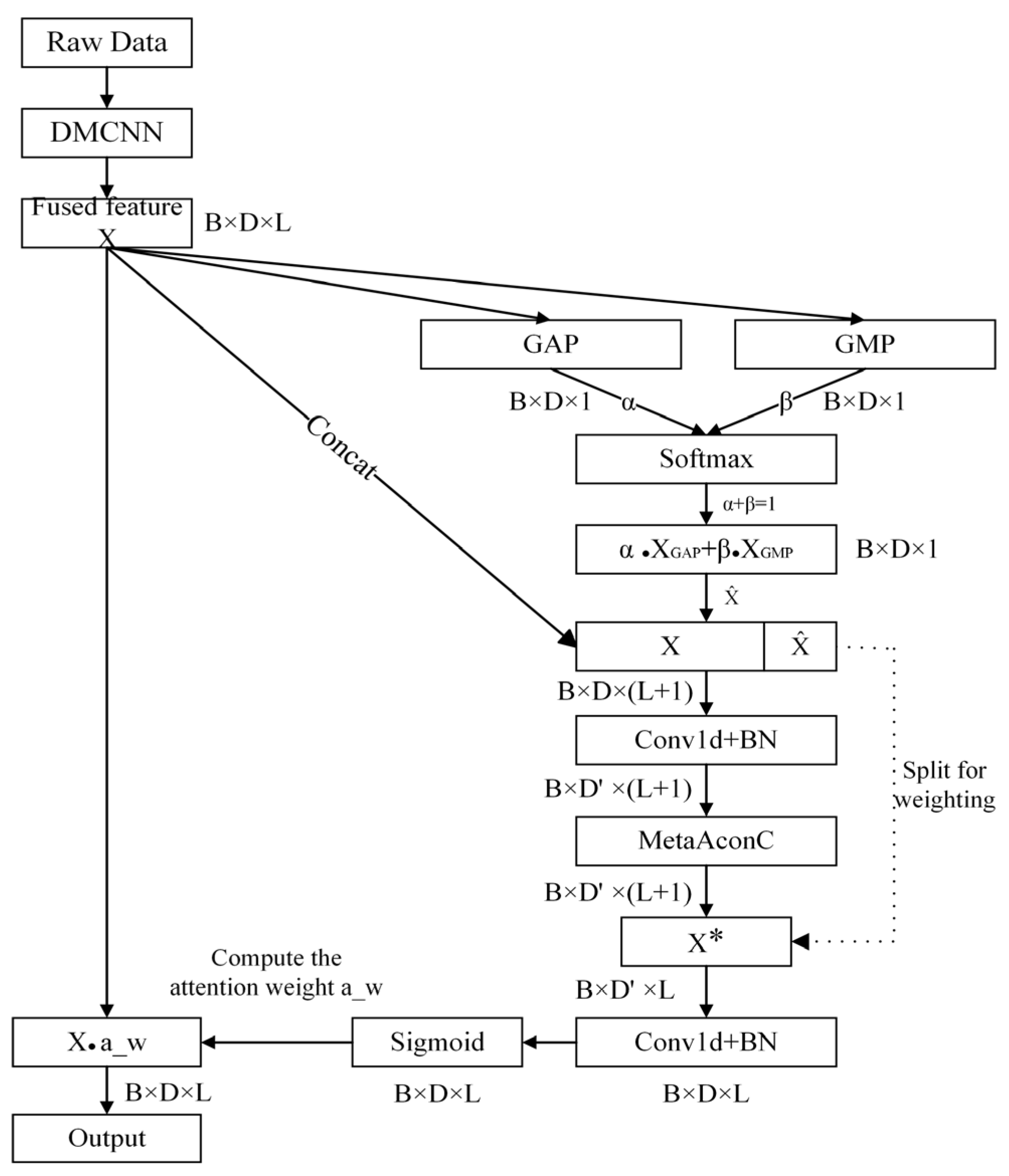
The specific structure of the CAM is illustrated in Figure 6. The fused input signal X needs to simultaneously capture long-term steady-state trends and transient anomalies in industrial process fault diagnosis. Hence, a dual-pooling strategy is employed. GAP calculates the mean value across each channel, focusing on global information and reflecting the overall operating condition of process variables, which is suitable for detecting long-term drifts. GMP computes the maximum value in each channel, which highlights abrupt transient changes. Therefore, it is particularly appropriate for identifying sudden anomalies. For the c-th channel, the outputs of GAP and GMP are computed as follows:

$$Y_{GAP}^c={\displaystyle \frac{1}{L}}{\displaystyle \sum _{l=1}^L{X}_{(c,l)}}$$

(16)

$$Y_{GMP}^c={\max }_{l=1}^L{X}_{(c,l)}$$

(17)

After the global pooling operation, the outputs of GAP and GMP are weighted and fused with the learnable parameters α and β, in which the initial sizes are both 0.5, and the sum of α and β is constrained to be 1 by the softmax function. Their relative weights are dynamically adjusted during training via backpropagation. This adaptive fusion method allows the model to extract global information without losing critical local features, thereby achieving optimal information integration and enhancing feature representation capability. The principle of weighted fusion is as follows:

$$\widehat{X}=\alpha \cdot Y_{GAP}+\beta \cdot Y_{GMP}$$

(18)

Furthermore, the original input features X are concatenated with the pooled $\widehat{X}$ to fully utilize the spatial location information and enrich the feature information. The combined feature is then processed by a 1 × 1 convolution operation H₁ to fuse the original input and pooled information while capturing inter-channel relationships. To encode channel dependencies, an intermediate feature connection matrix Q is generated, which is computed as follows:

$$Q=g[BN(H_1[Concat(X,\widehat{X})])]$$

(19)

where g represents the MetaAconC activation function.

The concatenated result is then split into $\widehat{X}$ and other parts. At this time, $\widehat{X}$ contains feature information of the original input as well as global information and key features after pooling. Next, 1 × 1 convolution operation H₂ is applied to project channels in $\widehat{X}$ back to their original dimensionality and generate the attention weights. Then, the weight values are mapped to the interval (0, 1) by a sigmoid function σ, which indicates the importance of each spatial location. Finally, each channel of the original input X_c is reweighted using the attention weights to generate the final output Y_c. Y_c is calculated as follows:

$$Wc=\sigma (BN[H_2(\widehat{X})])$$

(20)

$$Y\mathrm{c}=Wc\otimes Xc$$

(21)

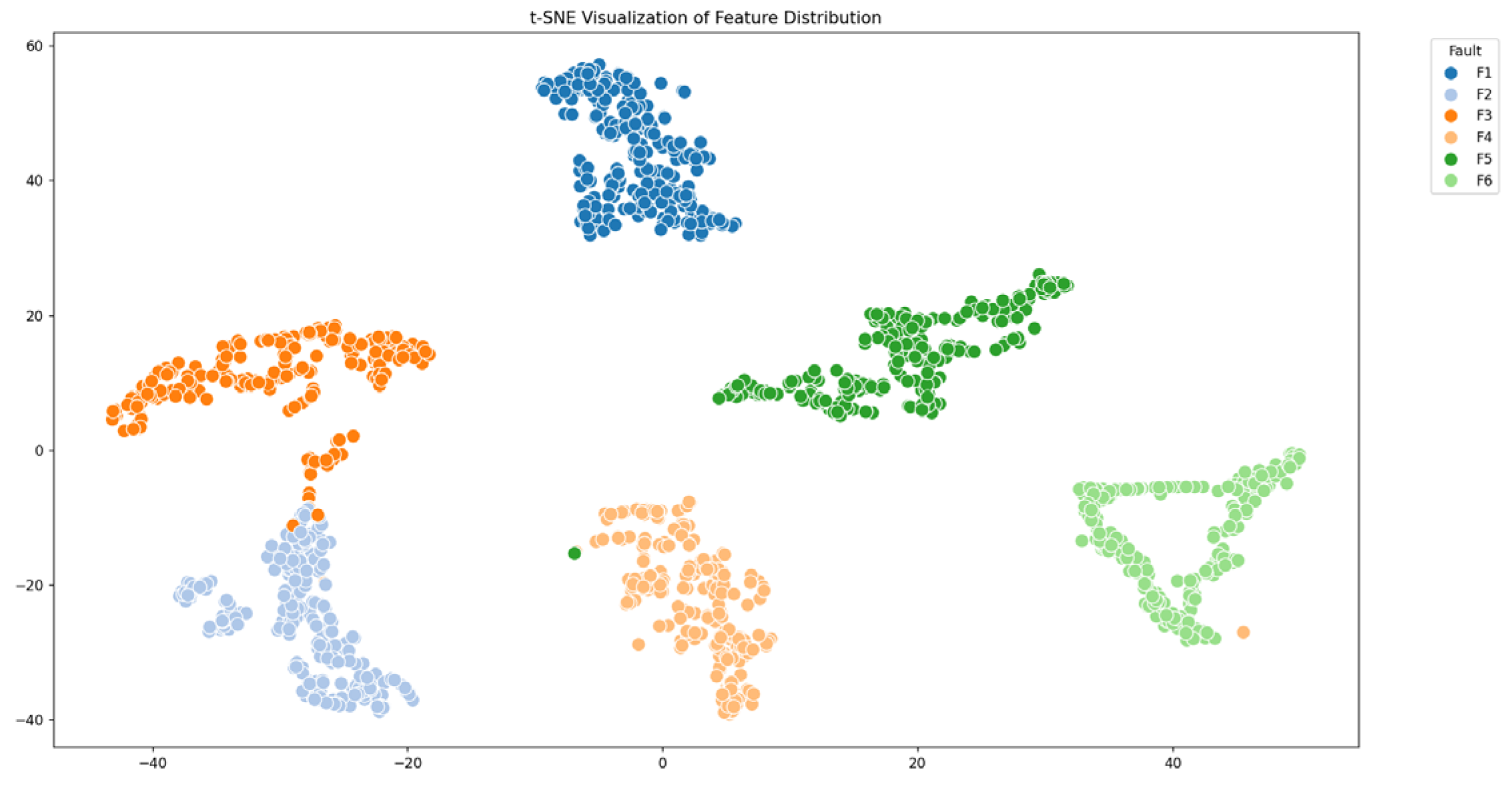
The CAM combines global average pooling and max pooling, and it introduces learnable parameters to adaptively balance their contributions, enabling the generation of differentiated weight coefficients for each input channel. This effectively reflects the contribution of each variable to the current fault mode. As a result, during prediction, the model can highlight key variables that are sensitive to faults while also providing quantifiable weight information for subsequent visualization and interpretability analysis, making it easier to explain the model’s diagnostic logic. In addition, the CAM concatenates the input with the pooled features and applies lightweight convolution together with the MetaAconC activation function, which enhances nonlinear feature representation while preserving local positional information and global statistical context. Compared with traditional attention mechanisms that only apply channel-wise weighting, this design maintains high efficiency and lightweight computation, while also retaining spatial information and enabling an adaptive focus on critical features. Therefore, the CAM not only strengthens the relevance and effectiveness of feature extraction but also significantly improves the interpretability and traceability of the model outputs, which helps to understand the diagnostic basis and decision-making process for different fault types.

3.3. BiGRU Module

To solve the problem of classifying time series, this paper employs a BiGRU module, which captures both forward and backward dependencies of the time series. Such a bidirectional modeling approach allows the model to acquire richer contextual information at each time step, thereby enhancing its ability to understand and predict sequence data.

Recurrent neural networks (RNNs) are capable of handling sequential data. Nevertheless, they are vulnerable to the vanishing or exploding gradient during long sequence processing, which makes it challenging for the model to capture long-term dependencies. To tackle this issue, long short-term memory (LSTM) was proposed on the basis of RNNs. 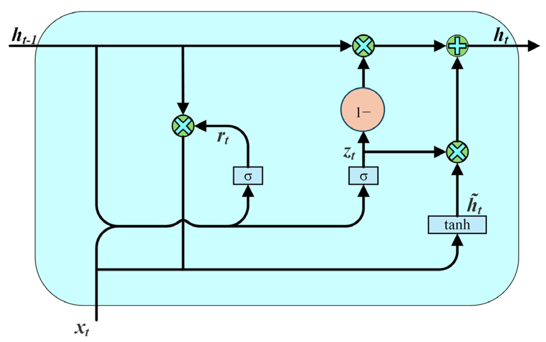By introducing the gating mechanism, LSTM can more effectively capture long-distance dependencies and mitigate the vanishing and exploding gradient caused by RNNs [43]. Based on LSTM, the GRU further simplifies the structure by merging the input and forget gates into a single update gate and introducing a reset gate to control the propagation of information. The GRU retains the core capabilities of LSTM while using fewer parameters and achieving faster training [44]. Its structure is shown in Figure 7, and its related computational flow is described in Equations (22)–(25):

$$z_t=\sigma (W_z\cdot [h_{t-1},x_t])$$

(22)

$$r_t=\sigma (W_r\cdot [h_{t-1},x_t])$$

(23)

$${\tilde{h}}_t=\tanh (W\cdot [r_t\ast h_{t-1},x_t])$$

(24)

$$h_t=(1-z_t)\ast h_{t-1}+z_t\ast {\tilde{h}}_t$$

(25)

where W_z, W_r, and W refer to weight matrices, σ represents the sigmoid activation function, x_t represents the input to the network at the current moment t, $\tilde{h}t$ is the candidate hidden state at time t, h_t−1 represents the previous hidden state, h_t denotes the hidden state at the current time t, and z_t and r_t refer to the update gate and reset gate, respectively. [·] denotes connecting two vectors, and * represents the product between matrix elements. The update gate is used to control how much information from the last hidden state is retained to the current moment. If z_t is close to 1, it means that most of the information from h_t−1 will be retained to the current moment. The reset gate controls the proportion of hidden information in the previous time step that should be forgotten. If r_t approaches 1, more information from the past hidden state is preserved.

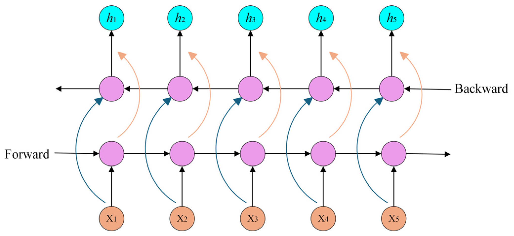
However, the traditional GRU can only process sequential information in a single direction along the time dimension. The fault characteristics of industrial equipment typically exhibit bidirectional temporal dependencies. For this reason, the BiGRU architecture is adopted in this study, and the schematic of its structure is depicted in Figure 8. The forward GRU processes the input features from past to future, while the backward GRU processes them from future to past. This bidirectional mechanism enables the output h_t at each time step to be composed of both a forward hidden state $\overrightarrow{h_t}$ and a reverse hidden state $\overleftarrow{h_t}$, which are calculated as follows:

$$\overrightarrow{h_t}=G(x_t,\overrightarrow{h_{t-1}})$$

(26)

$$\overleftarrow{h_t}=G(x_t,\overleftarrow{h_{t-1}})$$

(27)

$$h_t=w_t\overrightarrow{h_t}+v_t\overleftarrow{h_t}+b_t$$

(28)

where G(·) denotes the GRU computational process, $\overrightarrow{h_{t-1}}$ denotes the forward hidden state at the preceding time step, $\overleftarrow{h_{t-1}}$ represents previous backward hidden states, W_t is the weight of the forward hidden state, v_t corresponds to the weights of the backward hidden state, and b_t refers to the bias term.

3.4. Classification Module

The classification module is composed of four key components: a GAP layer, a fully connected (FC) layer, a dropout layer, and a softmax layer. The application of GAP before the fully connected (FC) layer serves two primary purposes: on the one hand, it reduces the model complexity and prevents overfitting; on the other hand, it is able to extract the global features of the timing information captured by the BiGRU module. After the FC layer merges features using a weight matrix, the number of parameters increases significantly, so the dropout layer is employed to prevent overfitting and enhance the model’s generalization ability. The merged features are then passed to a softmax classifier for category prediction. Instead of using standard cross-entropy loss, LSR is employed on top of it to soften the label distribution, improving robustness. Finally, the model is optimized by minimizing the loss function through backpropagation with the help of an optimization algorithm.

3.5. Fault Diagnosis Process

Figure 9 illustrates the overall framework for fault diagnosis. The fault diagnosis process contains offline modeling and online diagnosis.

Offline modeling stage:

Step 1: Acquire historical data from industrial processes, label the data, and randomly shuffle the dataset.

Step 2: Data preprocessing. Apply min–max normalization to scale the historical data into the [0, 1] range, and divide the dataset into training and testing sets.

Step 3: The DMCA-BiGRUN is established and trained on the training set.

Step 4: Feed the testing data into the trained model and evaluate the model performance. If the performance is suboptimal, continue to adjust model parameters. The best-performing model is saved whenever the performance improves.

Online diagnosis stage:

Step 1: Acquire the real-time industrial process monitoring data.

Step 2: The unlabeled data are normalized utilizing the min–max standardization method as the offline modeling stage.

Step 3: The preprocessed online data are fed into the trained DMCA-BiGRUN model to perform online diagnosis and identify fault types.

4. Simulation Experiments

In this section, the proposed DMCA-BiGRUN is employed in the TE process and the CSTR process to validate its performance. Three groups of ablation experiments and three deep learning models for fault diagnosis are used for comparison experiments. The ablation models are as follows: (1) DMCAN: This model excludes the BiGRU module while keeping the same parameter settings as DMCA-BiGRUN. (2) DCA-BiGRUN: This model replaces DMCNN with a standard CNN, using the same parameter settings as DMCA-BiGRUN. (3) DMC-BiGRUN: This model has the same parameter settings without using the CAM module. The comparative experimental model with the existing ones is as follows: (1) BCNN [45]; (2) ATT-1D CNN-GRU [46]; (3) MRCNN-LSTM [47].

Precision (P), recall (R), and the F1-score are employed as assessment indicators to evaluate the model’s performance. Precision reflects the model’s ability to correctly identify actual faulty samples among all samples it classifies as faulty. Recall indicates the ratio of correctly classified positive instances to the total number of true-positive instances. The F1-score combines precision and recall via their harmonic mean, which helps ensure a comprehensive evaluation of model performance in the case of category imbalance, avoiding the one-sidedness of a single metric. An increasing F1-score generally suggests that the model is achieving a better balance between precision and recall, which in turn reflects an improvement in overall performance. The relevant calculation formulas are as follows:

$$P={\displaystyle \frac{TP}{TP+FP}}$$

(29)

$$R={\displaystyle \frac{TP}{TP+FN}}$$

(30)

$$F1={\displaystyle \frac{2TP}{2TP+FP+FN}}$$

(31)

where true positive (TP) denotes the number of instances in which the model correctly classifies positive instances as positive, false positive (FP) refers to the number of negative instances that are incorrectly classified as positive, and false negative (FN) represents the number of positive instances that are mistakenly predicted as negative.

4.1. TE Process Simulation Experiments

4.1.1. Data Description

The TE Simulation Platform is a chemical process simulation model developed by Eastman Chemical Company in the United States. It simulates a real-world integrated chemical reaction process and is widely used as a benchmark for evaluating the performance of fault diagnosis methods in chemical processes. The specific process flow diagram is illustrated in Figure 10. It primarily includes five operating units: condenser, recirculation compressor, reactor, separator, and stripper tower. The TE process contains a total of 12 manipulated variables and 41 measured variables, and the detailed description can be found in [48]. There are 21 fault types for the TE simulation process, and fault descriptions are given in reference [49].

Based on the previous studies and analyses, 17 representative fault types are reasonably selected for this research. During the construction of the dataset, the sampling frequency is set to 30 samples per hour. For Fault 6, a total of 123 training samples and 247 testing samples are obtained, whereas each of the remaining 16 fault types has 1000 training samples and 2000 testing samples. In total, the dataset contains 17,123 training samples and 34,247 testing samples, including 1 healthy condition sample set and 16 fault condition sample sets.

4.1.2. Introduction to Model Parameters

To verify the rationality of the model’s architectural parameter settings, a sensitivity analysis was conducted on the convolution kernel sizes of the dual-path structure and the hidden dimension of the BiGRU. Specifically, for the coarse-grained path, large kernel sizes of 1 × 16, 1 × 17, 1 × 18, and 1 × 19 were tested, along with medium-sized kernels of 1 × 5, 1 × 7, and 1 × 9. For the fine-grained path, four-layer convolutional structures with kernel sizes of 1 × 3, 1 × 4, and 1 × 5 were evaluated. The BiGRU hidden dimensions were set to 32, 64, 128, and 256. For each configuration, classification accuracy was used as the performance metric to generate 3D surface plots, illustrating how accuracy changes with different kernel sizes and BiGRU dimensions. As shown in Figure 11, the combination of kernel sizes 1 × 17 and 1 × 9 for the coarse-grained path, 1 × 5 for the fine-grained path, and a BiGRU hidden size of 64 achieved the best performance in the experiments. This configuration not only ensures model stability but also significantly improves fault diagnosis accuracy. Therefore, this configuration is adopted as the default setup for subsequent experiments.

Based on the above sensitivity analysis, the final model architecture is constructed as follows. The standard convolutional layer employs 64 convolution kernels with a size of 1×7. The mixed convolution module consists of a coarse-grained path and a fine-grained path, which use the number of convolutional kernels of 50, 30 (of sizes 1 × 17 and 1 × 9), and 50, 40, 30, and 30 (both of size 1 × 5), respectively. For the time-series modeling part, the BiGRU with a hidden layer dimension of 64 is utilized. After GAP, the output is input to a fully connected layer with 128 units, and then a dropout layer with a 0.5 dropout rate is applied. The training of the model employs the AdamP optimizer with a batch size of 32, starting with an initial learning rate of 0.001 and every 30 batches decaying to 1/10 of the original one, with a total of 110 training batches.

4.1.3. Ablation Experiments

The simulation results of the DMCA-BiGRUN with three ablation models in the TE process fault diagnosis task are presented in

Table 1. Comparison of ablation experimental simulation results on TE process.

Fault Number	DMCAN (%)			DMC-BiGRUN (%)			DCA-BiGRUN (%)			DMCA-BiGRUN (%)
	P	R	F1	P	R	F1	P	R	F1	P	R	F1
1	98.65	98.70	98.68	99.05	98.75	98.90	98.60	98.80	98.70	99.05	99.55	99.30
2	99.64	98.05	98.84	99.14	97.45	98.29	96.00	98.40	97.19	99.05	98.65	98.85
4	97.76	96.00	96.87	95.18	94.75	94.96	98.44	97.85	98.14	99.35	98.90	99.12
5	98.41	99.20	98.80	99.06	99.60	99.33	98.91	99.50	99.20	99.70	99.75	99.73
6	100.00	95.14	97.51	99.17	96.76	97.95	100.00	100.00	100.00	100.00	99.19	99.59
7	100.00	100.00	100.00	100.00	99.95	99.98	100.00	100.00	100.00	100.00	100.00	100.00
8	91.62	83.05	87.12	86.31	77.20	81.50	87.44	81.45	84.34	98.24	83.50	90.27
10	89.38	87.55	88.46	86.21	82.20	84.16	88.64	91.25	89.92	98.02	94.30	96.13
11	80.71	69.65	74.77	82.57	67.25	74.13	93.33	81.80	87.18	95.72	89.45	92.48
12	86.94	91.20	89.02	86.45	92.20	89.23	90.11	92.05	91.07	93.52	96.05	94.77
13	87.44	76.25	81.46	81.99	71.00	76.10	88.99	67.10	76.51	85.12	88.35	86.70
14	67.66	80.45	73.50	70.91	78.50	74.51	84.97	94.10	89.30	93.56	95.20	94.37
16	70.01	82.60	75.78	59.49	82.25	69.05	76.16	85.30	80.47	84.13	97.25	90.21
17	91.06	85.05	87.95	89.64	85.70	87.63	94.49	94.25	94.37	95.40	98.55	96.95
18	94.76	94.85	94.80	95.32	93.75	94.53	95.31	96.45	95.87	97.70	95.75	96.72
19	98.29	97.45	97.87	96.75	96.75	96.75	96.86	95.75	96.30	95.01	97.10	96.04
20	85.32	90.95	88.04	86.38	86.25	86.31	84.71	96.10	90.04	98.58	97.00	97.78
Average	90.45	89.77	89.97	89.04	88.25	88.43	92.53	92.36	92.27	96.01	95.80	95.82

. As shown in the table, the proposed model attains an average recall rate of 95.8%, which is markedly superior to other models, thereby validating the effectiveness of each key module. The average recall of the DMCAN decreases by 6.03% (to 89.77%) after the BiGRU module is removed, indicating that BiGRU plays a crucial role in modeling temporal dependencies. The TE process data has strong temporal correlations. BiGRU can model forward and backward dependencies simultaneously, which helps to identify dynamic changes caused by faults. The DCA-BiGRUN replaces the DMCNN with a CNN, which leads to a decrease of 3.44% in the average recall, suggesting that the mixed convolution structure is more advantageous in feature extraction. It allows parallel extraction of multi-scale information and is more suitable for obtaining both local and global dynamic features in industrial processes. The absence of the CAM in the DMC-BiGRUN results in a 7.55% decrease in average recall, which highlights its importance in focusing on critical channels. By integrating spatial and channel information, the CAM improves the discriminative ability of the feature representation, enabling a more accurate classification of complex fault types. It is clear that the mixed convolution, CAM, and BiGRU modules form a synergistic combination for feature extraction, channel modeling, and temporal modeling, significantly enhancing the model’s fault identification capability in complex dynamic industrial processes.

To highlight the advantages of the proposed model in parameter optimization compared to CNN, this study compares the DCA-BiGRUN and DMCA-BiGRUN models in terms of the total number of parameters, total training time (over 110 batches), and average inference time per sample. The results are summarized in

Table 2. Total parameters and training/testing time of model on the TE process.

	DCA-BiGRUN	DMCA-BiGRUN
Training time	12.27 min	25.47 min
Testing time	0.0124 s	0.0243 s
Total parameters	78,563	32,069

. The proposed DMCA-BiGRUN contains only about 41% of the parameters of the DCA-BiGRUN, which shows a significant reduction in model parameters. Although its training time and testing time are relatively long, this is mainly due to the more complex path design and feature fusion process in the mixed convolution structure. Nevertheless, the performance of the model is improved. Considering that the training process is usually offline and the one-time training cost has a limited impact on the practical application, the result is acceptable overall. DMCA-BiGRUN requires only about 0.0243 s to test a single sample and still maintains high inference efficiency, which makes it suitable for real-time fault detection tasks.

To further analyze the feature representation capability of the proposed DMCA-BiGRUN in TE progress fault diagnosis tasks, t-distributed stochastic neighbor embedding (t-SNE) is applied to visualize the high-dimensional features extracted by the model. These features are projected into a two-dimensional space to intuitively display the clustering effectiveness of distinct fault categories. The visualization result is shown in Figure 12. The samples of the same fault category are clearly clustered and the different categories are well separated from each other, reflecting a strong discriminative ability. Figure 13 presents the confusion matrices of the proposed DMCA-BiGRUN and the ablation models. Although certain confusions still exist among Faults 8, 11, 13, and 16, the proposed model achieves a higher accuracy in identifying these faults compared to other models, demonstrating a superior fault recognition performance.

4.1.4. Robustness Evaluation Under Gaussian Noise

To assess the robustness of the proposed DMCA-BiGRUN under uncertainty and interference, we conducted experiments by adding zero-mean Gaussian noise with varying standard deviations δ to the dataset. Specifically, δ was set to 0.001, 0.002, and 0.003 to simulate different intensities of measurement noise and external disturbances commonly encountered in real-world industrial environments.

The results of the experiments are presented in

Table 3. Performance of the proposed DMCA-BiGRUN under different levels of Gaussian noise in the TE process.

Noise Level (δ)	Accuracy (%)	F1-Score (%)
0 (no noise)	96.01	95.82
0.001	95.17	95.12
0.002	94.88	94.86
0.003	94.50	94.49

. It can be observed that the proposed DMCA-BiGRUN exhibits strong robustness under increasing levels of Gaussian noise. When no noise is added (δ = 0), the model achieves an accuracy of 96.01% and an F1-score of 95.80%. As the noise level increases to 0.003, the accuracy and F1-score decrease only slightly to 94.50% and 94.49%, respectively.

These results indicate that the performance degradation is minimal even under noisy conditions, suggesting that the model maintains a reliable classification capability in the presence of measurement disturbances. This robustness is essential for real-world applications where sensor noise and process fluctuations are inevitable.

4.1.5. Comparison Experiments

The test accuracy curves of the proposed model and the existing models BCNN, ATT-1D CNN-GRU, and MRCNN-LSTM applied to the TE process fault diagnosis task are shown in Figure 14. As shown by the red line in the figure, the proposed model demonstrates a significant advantage over the other three methods in accuracy after 27 epochs. Moreover, the accuracy of the proposed DMCA-BiGRUN stabilizes after 45 epochs, while the other models exhibit greater fluctuations and require more time to converge, indicating that the proposed model is more stable. When comparing the accuracy of the four models after convergence, the proposed model still shows a more effective capacity for fault distinction. Figure 15 presents the F1-score of each model for the easily confused faults 8, 11, 13, and 16 in this case, and the F1-scores of the proposed model reach 90.27%, 92.48%, 86.7%, and 90.21%, respectively, which significantly surpass the other three groups of comparison models, demonstrating that even in the diagnosis of confusing faults, DMCA-BiGRUN has a more accurate discriminative ability.

4.2. CSTR Process Simulation Experiments

4.2.1. Data Description

The CSTR is a complex nonlinear chemical reactor system, which is centrally characterized by simultaneous feeding, reaction, and discharge. Sufficient mixing is achieved by stirring in the reactor to ensure a uniform concentration and temperature [50]. The process flow diagram is shown in Figure 16. The balance equations for the material and energy of the reactant are formulated in Equations (32) and (33).

$$V_r{\displaystyle \frac{d{C}_r}{dt}}=F(C_{in}-C_r)-V_r{k}_r{C}_r$$

(32)

$$\rho C_p{V}_r{\displaystyle \frac{dT}{dt}}=F\rho C_p(T_{in}-T)+(-\Delta H_r)V_r{k}_r{C}_r-UA(T-T\mathrm{c})$$

(33)

where C_in is the concentration of the reactant in the feed, C_r refers to the reactant concentration inside the reactor, F represents the flow rate, V_r denotes the reactor’s volume, k_r refers to the reaction rate constant, ρ represents the mixture density during the reaction, C_p stands for the mixture’s specific heat capacity at a constant pressure, T_in is the temperature of the feed stream, T is the temperature inside the reactor, −ΔH_r denotes the enthalpy change of the reaction, UA denotes the product of the overall heat transfer coefficient U and the heat transfer area A, and Tc is the temperature of the cooling medium.

In this study, the CSTR simulation process proposed by Yoon and MacGregor is employed to verify the feasibility of the proposed DMCA-BiGRUN [51]. Nine process variables of the system are selected, as shown in

Table 4. Measured variables of the CSTR process.

Variable Number	Variable Name	Variable Number	Variable Name
1	Temperature of the mixture in the reactor T	6	Concentration of reactants in the reactor CA
2	Temperature of the raw material stream TF	7	Outlet flow rate Q
3	Temperature of the coolant in the cooling jacket TC	8	Coolant flow rate QC
4	Inlet temperature of the coolant TCF	9	Feed flow rate into the reactor QF
5	Concentration of reactants in the feed stream CAF

. These nine variables are used to identify six types of faults in the CSTR process, with fault descriptions provided in

Table 5. Fault descriptions of the CSTR process.

Fault Number	Fault Description	Fault Magnitude
1	T Random disturbance	U(2, 4)
2	CAF Step change	1.0 kmol/m3
3	CAF Ramp change	dCAF/dt = 0.2 kmol/(m3·min)
4	k0 Slow drift	k0(t + 1) = 0.996 × k0(t)
5	Heat exchanger fouling	UAC = UAC −120 J/(min−2·K)
6	QC Random noise	N (0, 5)

. The system tracks the variables over 250 min at a sampling frequency of 1 min, obtaining 250 training samples for each fault. For testing, it collects 500 samples over 500 min, with faults introduced starting from the 151st sample. In total, 1750 training samples and 3500 testing samples were collected, including one normal sample set and six faulty sample sets.

4.2.2. Ablation Experiments

The results of the t-SNE visualization of the CSTR process can be found in Figure 17. The figure demonstrates that the proposed DMCA-BiGRUN exhibits strong classification capabilities. The results of the proposed model and its three ablation comparison models in the CSTR process fault diagnosis task are summarized in

Table 6. Comparison of ablation experimental simulation results on CSTR process.

Fault Number	DMCAN (%)			DMC-BiGRUN (%)			DCA-BiGRUN (%)			DMCA-BiGRUN (%)
	P	R	F1	P	R	F1	P	R	F1	P	R	F1
1	100.00	100.00	100.00	100.00	100.00	100.00	100.00	100.00	100.00	100.00	100.00	100.00
2	89.29	100.00	94.34	88.97	99.14	93.78	93.82	99.71	96.68	95.11	100.00	97.49
3	98.99	84.00	90.88	97.99	83.71	90.29	98.76	91.14	94.80	99.70	93.71	96.61
4	95.71	95.71	95.71	94.84	94.57	94.71	97.71	97.71	97.71	98.86	98.86	98.86
5	98.31	99.71	99.01	100.00	98.86	99.43	99.71	99.43	99.57	100.00	99.43	99.71
6	94.10	95.71	94.90	91.53	95.71	93.58	97.75	99.43	98.58	98.59	100.00	99.29
Average	96.07	95.86	95.81	95.56	95.33	95.30	97.96	97.90	97.89	98.71	98.67	98.66

. It is worth noting that the DMCA-BiGRUN has the highest average precision, recall, and F1-score. Compared with the other three ablation models, it also maintains a high diagnostic accuracy for each fault category. For a more intuitive comparison, the confusion matrices of the four models are presented in Figure 18.

4.2.3. Robustness Evaluation Under Gaussian Noise

Table 7. Performance of the proposed DMCA-BiGRUN under different levels of Gaussian noise in the CSTR process.

Noise Level (δ)	Accuracy (%)	F1-Score (%)
0 (no noise)	98.71	98.66
0.001	99.00	99.00
0.002	98.86	98.86
0.003	98.29	98.28

demonstrates the fault diagnosis results of the proposed model under different noise levels in the CSTR process. It can clearly be seen that the proposed DMCA-BiGRUN maintains an outstanding classification performance under different levels of Gaussian noise. Notably, the model achieved a slightly better performance when Gaussian noise with 0.001 or 0.002 was added compared to the noiseless setting. At δ = 0.001, the model achieved its best performance, attaining 99.00% in both accuracy and F1-score. This improvement indicates that slight noise can serve as implicit regularization, enhancing generalization by mitigating overfitting. As the noise intensity increases to 0.003, the performance declines slightly but still remains highly robust, with the accuracy and F1-score approaching 98.3%. These results highlight the strong noise tolerance and generalization ability of the DMCA-BiGRU model at these noise levels.

4.2.4. Comparison Experiments

To verify the effectiveness and superiority of the proposed method, two additional comparative models were included in the experiments. The comparative results of the proposed DMCA-BiGRUN with five methods, CNN-GRU, MRCNN, BCNN, ATT-1D CNN-GRU, and MRCNN-LSTM, in the CSTR process fault diagnosis task are presented in

Table 8. Comparative experimental results of the six models on CSTR process.

Fault Type	CNN-GRU (%)			MRCNN (%)			BCNN (%)			ATT-1D CNN-GRU (%)			MRCNN-LSTM (%)			DMCA-BiGRUN (%)
	P	R	F1	P	R	F1	P	R	F1	P	R	F1	P	R	F1	P	R	F1
1	100.00	100.00	100.00	100.00	100.00	100.00	100.00	100.00	100.00	100.00	100.00	100.00	100.00	100.00	100.00	100.00	100.00	100.00
2	90.21	100.0	94.85	91.30	96.00	93.59	89.90	99.14	94.29	90.60	99.14	94.68	90.84	99.14	94.81	95.11	100.00	97.49
3	98.99	84.29	91.05	95.78	84.29	89.67	98.66	84.00	90.74	98.01	84.57	90.80	99.01	85.71	91.88	99.70	93.71	96.61
4	96.64	90.29	93.35	89.12	98.29	93.48	93.91	96.86	95.36	96.84	96.29	96.56	94.59	100.00	97.22	98.86	98.86	98.86
5	96.13	99.43	97.75	96.65	98.86	97.74	98.85	98.57	98.71	100.00	99.14	99.57	99.71	99.14	99.43	100.00	99.43	99.71
6	87.47	93.71	90.48	95.45	90.00	92.65	93.26	94.86	94.05	92.43	97.71	95.00	98.56	97.71	98.13	98.59	100.00	99.29
Avg	94.91	94.62	94.58	94.72	94.57	94.52	95.76	95.57	95.53	96.31	96.14	96.10	97.12	96.95	96.91	98.71	98.67	98.66

. The proposed DMCA-BiGRUN attains the highest precision and recall across all fault types among the six models. Notably, for fault 3, which is the most difficult to distinguish, the proposed model achieves an F1-score of 96.61%, surpassing the other models. These results indicate that the proposed DMCA-BiGRUN offers a superior fault discrimination ability and further verify its feasibility and superiority.

5. Conclusions

This paper proposes an industrial fault diagnosis method based on a dual-path mixed convolutional attention-BiGRU (DMCA-BiGRUN). The dual-path mixed convolution extracts multi-scale features through two parallel convolutional branches with different kernel sizes. By integrating depthwise convolution, residual connections, and pointwise convolution, it effectively addresses the limitations of a CNN, which typically extracts only local features with high parameter overheads, and it enhances the learning of multi-variate coupling features in complex industrial processes. The CAM combines GAP and GMP through weighted fusion, preserving global channel information and key features while incorporating positional information to reweight the original features. This allows the model to adaptively concentrate on crucial feature information. The BiGRU module captures forward and backward dependencies in the sequence, allowing the model to consider bidirectional information flow at each time step. This results in more comprehensive contextual information and helps mitigate gradient vanishing issues caused by long sequence lengths during training. Finally, simulation experiments on the TE and CSTR processes validate the feasibility and superiority of the proposed model.

References

1. Gui, X.; Zhang, J.; Tang, J.; Xu, H.; Zou, J.; Fan, S. A Quadruplet Deep Metric Learning Model for Imbalanced Time-Series Fault Diagnosis. Knowl. Based Syst. 2022, 238, 107932. [Google Scholar] [CrossRef]
2. Chen, Y.; Zhang, C.; Zhang, R.; Gao, F. Deep Network Model Fusion of Wide Kernel Feature Learning for Industrial Process Modeling and Fault Diagnosis. Process Saf. Environ. Prot. 2025, 194, 1283–1302. [Google Scholar] [CrossRef]
3. Chen, K.; Wang, W.; Zhang, F.; Liang, J.; Yu, K. Correlation-Guided Particle Swarm Optimization Approach for Feature Selection in Fault Diagnosis. IEEE/CAA J. Autom. Sin. 2025, 1–13. [Google Scholar] [CrossRef]
4. Márquez-Vera, M.A.; Ramos-Velasco, L.E.; López-Ortega, O.; Zúñiga-Peña, N.S.; Ramos-Fernández, J.C.; Ortega-Mendoza, R.M. Inverse Fuzzy Fault Model for Fault Detection and Isolation with Least Angle Regression for Variable Selection. Comput. Ind. Eng. 2021, 159, 107499. [Google Scholar] [CrossRef]
5. Sadhukhan, C.; Mitra, S.K.; Naskar, M.K.; Sharifpur, M. Fault Diagnosis of a Nonlinear Hybrid System Using Adaptive Unscented Kalman Filter Bank. Eng. Comput. 2022, 38, 2717–2728. [Google Scholar] [CrossRef]
6. Cao, Z.; Du, X. An Intelligent Optimization-Based Particle Filter for Fault Diagnosis. IEEE Access 2021, 9, 87839–87848. [Google Scholar] [CrossRef]
7. Zhang, S.; Zhai, X.; Wu, J. Application of Fault Tree Analysis in Fault Diagnosis of Detectors in Nuclear Power Plant. In Proceedings of the 2023 CAA Symposium on Fault Detection, Supervision and Safety for Technical Processes (SAFEPROCESS), Yibin, China, 22–24 September 2023; pp. 1–5. [Google Scholar]
8. Gonzalez-Jimenez, D.; Del-Olmo, J.; Poza, J.; Garramiola, F.; Madina, P. Data-Driven Fault Diagnosis for Electric Drives: A Review. Sensors 2021, 21, 4024. [Google Scholar] [CrossRef] [PubMed]
9. Yang, J.; Wang, J.; Sha, J.; Dai, H.; Liu, H. Quality-Related Monitoring of Distributed Process Systems Using Dynamic Concurrent Partial Least Squares. Comput. Ind. Eng. 2022, 164, 107893. [Google Scholar] [CrossRef]
10. Khan, M.M.; Islam, I.; Rashid, A.B. Fault Diagnosis of an Industrial Chemical Process Using Machine Learning Algorithms: Principal Component Analysis (PCA) and Kernel Principal Component Analysis (KPCA). In IOP Conference Series: Materials Science and Engineering; IOP Publishing: Bristol, UK, 2024; Volume 1305, p. 012037. [Google Scholar]
11. Jiang, Q.; Wang, W.; Chen, S.; Pan, C.; Zhong, W. Hierarchical Fault Root Cause Identification in Plant-Wide Processes Using Distributed Direct Causality Analysis. IEEE Trans. Ind. Inform. 2023, 20, 3232–3241. [Google Scholar] [CrossRef]
12. Chen, Y.; Zhang, X.; Li, D.; Zhou, J. A New Class of Fault Detection and Diagnosis Methods by Fusion of Spatially Distributed and Time-Dependent Features. J. Process Control 2025, 146, 103372. [Google Scholar] [CrossRef]
13. Li, C.; Liu, J.; Yang, X.; Wei, Y.; Wu, Z.; Li, M. The PCA Fault Diagnosis Method Based on Causal Relationships. In Proceedings of the 2024 3rd International Conference on Automation, Robotics and Computer Engineering (ICARCE), Virtual, 17–18 December 2024; pp. 340–344. [Google Scholar]
14. Xiu, X.; Miao, Z. Robust Sparse Canonical Correlation Analysis: New Formulation and Application to Fault Detection. IEEE Sens. Lett. 2022, 6, 1–4. [Google Scholar] [CrossRef]
15. Wang, Q.; Wang, S.; Wei, B.; Chen, W.; Zhang, Y. Weighted K-NN Classification Method of Bearings Fault Diagnosis with Multi-Dimensional Sensitive Features. IEEE Access 2021, 9, 45428–45440. [Google Scholar] [CrossRef]
16. Yan, P.; Wang, J.; Wang, W.; Li, G.; Zhao, Y.; Wen, Z. Transformer Fault Diagnosis Based on MPA-RF Algorithm and LIF Technology. Meas. Sci. Technol. 2023, 35, 025504. [Google Scholar] [CrossRef]
17. Wang, G.; Tu, Y.; Nie, J. An Analog Circuit Fault Diagnosis Method Using Improved Sparrow Search Algorithm and Support Vector Machine. Rev. Sci. Instrum. 2024, 95, 055110. [Google Scholar] [CrossRef] [PubMed]
18. Cui, X.; Han, H.; Guo, X. Embedding Space Reconstruction to Enhance ANN for Industrial Process Fault Diagnosis. In Proceedings of the 2023 International Conference on Artificial Intelligence, Systems and Network Security, Mianyang, China, 22–24 December 2023; pp. 438–442. [Google Scholar]
19. Wu, H. Feature-Weighted Naive Bayesian Classifier for Wireless Network Intrusion Detection. Secur. Commun. Netw. 2024, 2024, 7065482. [Google Scholar] [CrossRef]
20. Ye, Z.; Wei, H. Gas Turbine Fault Diagnosis Based on IPSO-SVM. In Proceedings of the 2021 6th International Conference on Power and Renewable Energy (ICPRE), Shanghai, China, 17–20 September 2021; pp. 280–284. [Google Scholar]
21. Han, X.; Zhao, H.; Song, Y.; Sun, D.; Fan, Y. TE Process Fault Diagnosis Based on KPCA-RF. In Proceedings of the 2023 35th Chinese Control and Decision Conference (CCDC), Yichang, China, 20–22 May 2023; pp. 652–657. [Google Scholar]
22. Shen, G.; Wang, P.; Hu, K.; Ye, Q. Fault Root Cause Diagnosis Method Based on Recurrent Neural Network and Granger Causality. In Proceedings of the 2021 CAA Symposium on Fault Detection, Supervision, and Safety for Technical Processes (SAFEPROCESS), Chengdu, China, 17–18 December 2021; pp. 1–6. [Google Scholar]
23. Ran, R.; Wang, T.; Zhang, W.; Fang, B. Autoencoder-Based Discriminant Locality Preserving Projections for Fault Diagnosis. IEEE Trans. Instrum. Meas. 2025, 74, 1–13. [Google Scholar] [CrossRef]
24. Zhong, C.; Jiang, Y.; Wang, L.; Chen, J.; Zhou, J.; Hong, T.; Zheng, F. Improved MLP Energy Meter Fault Diagnosis Method Based on DBN. Electronics 2023, 12, 932. [Google Scholar] [CrossRef]
25. Kim, S.; Choi, J.-H. Convolutional Neural Network for Gear Fault Diagnosis Based on Signal Segmentation Approach. Struct. Health Monit. 2019, 18, 1401–1415. [Google Scholar] [CrossRef]
26. Niu, X.; Yang, X. A Novel One-dimensional Convolutional Neural Network Architecture for Chemical Process Fault Diagnosis. Can. J. Chem. Eng. 2022, 100, 302–316. [Google Scholar] [CrossRef]
27. Xing, J.; Xu, J. An Improved Convolutional Neural Network for Recognition of Incipient Faults. IEEE Sens. J. 2022, 22, 16314–16322. [Google Scholar] [CrossRef]
28. Song, Q.; Jiang, P. A Multi-Scale Convolutional Neural Network Based Fault Diagnosis Model for Complex Chemical Processes. Process Saf. Environ. Prot. 2022, 159, 575–584. [Google Scholar] [CrossRef]
29. Liang, H.; Zhao, X. Rolling Bearing Fault Diagnosis Based on One-Dimensional Dilated Convolution Network with Residual Connection. IEEE Access 2021, 9, 31078–31091. [Google Scholar] [CrossRef]
30. Zhou, K.; Tong, Y.; Li, X.; Wei, X.; Huang, H.; Song, K.; Chen, X. Exploring Global Attention Mechanism on Fault Detection and Diagnosis for Complex Engineering Processes. Process Saf. Environ. Prot. 2023, 170, 660–669. [Google Scholar] [CrossRef]
31. Sun, H.; Fan, Y. Fault Diagnosis of Rolling Bearings Based on CNN and LSTM Networks under Mixed Load and Noise. Multimed. Tools Appl. 2023, 82, 43543–43567. [Google Scholar] [CrossRef]
32. Xu, Z.; Li, C.; Wang, X.; Jin, J. Fault Diagnosis of Wind Turbine Bearing Using a Multi-Scale Convolutional Neural Network for Multi-Sensors. SSRN 2021. preprint. [Google Scholar] [CrossRef]
33. Zhang, J.; Zhang, M.; Feng, Z.; Ruifang, L.V.; Lu, C.; Dai, Y.; Dong, L. Gated Recurrent Unit-Enhanced Deep Convolutional Neural Network for Real-Time Industrial Process Fault Diagnosis. Process Saf. Environ. Prot. 2023, 175, 129–149. [Google Scholar] [CrossRef]
34. Cha, Y.-J.; Ali, R.; Lewis, J.; Büyükӧztürk, O. Deep Learning-Based Structural Health Monitoring. Autom. Constr. 2024, 161, 105328. [Google Scholar] [CrossRef]
35. Xu, Q.; Xing, Y.; Hu, J.; Jia, Y.; Huang, R. CEBSNet: Change-Excited and Background-Suppressed Network with Temporal Dependency Modeling for Bitemporal Change Detection. arXiv 2025, arXiv:2505.15322. [Google Scholar]
36. Lee, S.; Park, T.; Lee, K. Partial Channel Dependence with Channel Masks for Time Series Foundation Models. arXiv 2024, arXiv:2410.23222. [Google Scholar] [CrossRef]
37. Xiong, S.; Zhou, L.; Dai, Y.; Ji, X. Attention-Based Long Short-Term Memory Fully Convolutional Network for Chemical Process Fault Diagnosis. Chin. J. Chem. Eng. 2023, 56, 1–14. [Google Scholar] [CrossRef]
38. Zhang, J.; Wang, Y.; Tang, J.; Zou, J.; Fan, S. MS-TCN: A Multiscale Temporal Convolutional Network for Fault Diagnosis in Industrial Processes. In Proceedings of the 2021 American Control Conference (ACC), New Orleans, LA, USA, 25–28 May 2021; pp. 1601–1606. [Google Scholar]
39. Yang, S.; Li, P.; Li, S.; Zhou, X.; Jiang, S. Fault Diagnosis Based on Multi-Scale LSTM-FCNs for Industrial Process. In Proceedings of the 2021 CAA Symposium on Fault Detection, Supervision, and Safety for Technical Processes (SAFEPROCESS), Chengdu, China, 17–18 December 2021; pp. 1–6. [Google Scholar]
40. Du, B.; Li, W.; Qin, X. A Classification and Recognition Model for Multiple Fruit Tree Leaf Diseases. Environ. Res. Commun. 2024, 6, 105034. [Google Scholar] [CrossRef]
41. Liu, G.; Jiang, Q.; Sun, Y.; Song, X.; Tang, H.; Liu, Z.; Chen, Q. A Double-Branch Improved Residual Shrinkage Network for Diagnosis of Induction Motor Broken Rotor Bar Under Small Samples. IEEE Trans. Instrum. Meas. 2025, 74, 1–12. [Google Scholar] [CrossRef]
42. Feng, Y.; Chen, J.; Zhang, T.; He, S.; Xu, E.; Zhou, Z. Semi-Supervised Meta-Learning Networks with Squeeze-and-Excitation Attention for Few-Shot Fault Diagnosis. ISA Trans. 2022, 120, 383–401. [Google Scholar] [CrossRef] [PubMed]
43. Gu, X.; Hou, Z.; Cai, J. Data-Based Flooding Fault Diagnosis of Proton Exchange Membrane Fuel Cell Systems Using LSTM Networks. Energy AI 2021, 4, 100056. [Google Scholar] [CrossRef]
44. Han, S.; Wang, P.; Zhang, C.; Wang, J. Fault Diagnosis of Dynamic Chemical Processes Based on Improved Residual Network Combined with a Gated Recurrent Unit. ACS Omega 2025, 10, 8859–8869. [Google Scholar] [CrossRef] [PubMed]
45. Wang, N.; Li, H.; Wu, F.; Zhang, R.; Gao, F. Fault Diagnosis of Complex Chemical Processes Using Feature Fusion of a Convolutional Network. Ind. Eng. Chem. Res. 2021, 60, 2232–2248. [Google Scholar] [CrossRef]
46. Liu, H.; Ma, R.; Li, D.; Yan, L.; Ma, Z. Machinery Fault Diagnosis Based on Deep Learning for Time Series Analysis and Knowledge Graphs. J. Signal Process. Syst. 2021, 93, 1433–1455. [Google Scholar] [CrossRef]
47. Liu, K.; Lu, N.; Wu, F.; Zhang, R.; Gao, F. Model Fusion and Multiscale Feature Learning for Fault Diagnosis of Industrial Processes. IEEE Trans. Cybern. 2022, 53, 6465–6478. [Google Scholar] [CrossRef] [PubMed]
48. Xu, H.; Ren, T.; Mo, Z.; Yang, X. A Fault Diagnosis Model for Tennessee Eastman Processes Based on Feature Selection and Probabilistic Neural Network. Appl. Sci. 2022, 12, 8868. [Google Scholar] [CrossRef]
49. Yan, X.; Zhang, Y.; Jin, Q. Chemical Process Fault Diagnosis Based on Improved ResNet Fusing CBAM and SPP. IEEE Access 2023, 11, 46678–46690. [Google Scholar] [CrossRef]
50. Ding, Y.; Zhang, Y.; Huang, J.; Peng, S. Incremental Pyraformer–Deep Canonical Correlation Analysis: A Novel Framework for Effective Fault Detection in Dynamic Nonlinear Processes. Algorithms 2025, 18, 130. [Google Scholar] [CrossRef]
51. Yoon, S.; MacGregor, J.F. Fault Diagnosis with Multivariate Statistical Models Part I: Using Steady State Fault Signatures. J. Process Control 2001, 11, 387–400. [Google Scholar] [CrossRef]
Figure 1. CNN structure diagram.
Mathematics 13 02331 g001
Figure 2. Schematic diagram of max pooling.
Mathematics 13 02331 g002
Figure 3. Overall structure of DMCA-BiGRUN.
Mathematics 13 02331 g003
Figure 4. Architecture of DMCNN.
Mathematics 13 02331 g004
Figure 5. Structure of the mixed convolution.
Mathematics 13 02331 g005
Figure 6. Structure of the CAM.
Mathematics 13 02331 g006
Figure 7. GRU structure diagram.
Mathematics 13 02331 g007
Figure 8. BiGRU structure diagram.
Mathematics 13 02331 g008
Figure 9. Flowchart of the fault diagnosis process using the DMCA-BiGRUN model.
Mathematics 13 02331 g009
Figure 10. Flowchart of TE process.
Mathematics 13 02331 g010
Figure 11. Sensitivity analysis of dual-path convolution kernel sizes and BiGRU dimensions. In the figure, [(17, 9), 5] indicates that the coarse-grained path uses convolution kernels of sizes 1 × 17 and 1 × 9, while the fine-grained path uses convolution kernels of size 1 × 5.
Mathematics 13 02331 g011
Figure 12. t-SNE visualization result of DMCA-BiGRUN model for fault diagnosis in TE process.
Mathematics 13 02331 g012
Figure 13. Confusion matrices of the proposed model and ablation comparison models. (a) DMCA-BiGRUN; (b) DMCAN; (c) DMC-BiGRUN; (d) DCA-BiGRUN.
Mathematics 13 02331 g013
Figure 14. Test accuracy curves of the four models.
Mathematics 13 02331 g014
Figure 15. F1-scores of the four models in diagnosing faults 8, 11, 13, and 16.
Mathematics 13 02331 g015
Figure 16. Flowchart of CSTR process.
Mathematics 13 02331 g016
Figure 17. t-SNE visualization result of DMCA-BiGRUN model for fault diagnosis in CSTR process.
Mathematics 13 02331 g017
Figure 18. Confusion matrices of four models. (a) DMCA-BiGRUN; (b) DMCAN; (c) DMC-BiGRUN; (d) DCA-BiGRUN.
Mathematics 13 02331 g018