An Exponentially Delayed Feedback Chaotic Model Resistant to Dynamic Degradation and Its Application

Abstract

In this paper, an exponential delay feedback method is proposed to improve the performance of the digital chaotic maps against their dynamical degradation. In this paper, the performance of the scheme is verified using one-dimensional linear, exponential, and nonlinear exponential, Logistic, and Chebyshev maps, and numerical analyses show that the period during which the chaotic sequence enters the cycle is considerably prolonged, and the correlation performance is improved. At the same time, in order to verify the practicality of the method, an image encryption algorithm is designed, and its security analysis results show that the algorithm has a high level of security and can compete with other encryption schemes. Therefore, the exponential delay feedback method can effectively improve the dynamics degradation of a digital chaotic map.

1. Introduction

Chaotic maps themselves have highly complex properties, such as unpredictability, non-periodicity, pseudo-randomness, etc., which makes them extremely applicable in the field of image encryption. Ref. [1] uses a KAA map in conjunction with other maps in conjunction with each other to achieve encryption using bit obfuscation and diffusion. Ref. [2] constructed new 2D hyperchaotic maps from Schaffer functions applied to encryption.

Under normal circumstances, chaotic map is implemented on a device with limited precision, the state space becomes finite, which we call a digital chaotic map, and the output sequence generated on this basis will naturally exhibit periodicity, and the chaotic properties it possesses by itself will disappear, which is commonly referred to as dynamics degradation [3]. Therefore, encryption algorithms designed based on digital chaotic maps can lack security. With the emergence of this problem, many schemes to improve the degradation of the dynamics of existing chaotic map models have emerged [4,5,6,7,8,9]. For example, Ref. [4] proposed a universal shift coupling digital chaotic model to counteract dynamical degradation. Ref. [5] used the sinusoidal function as a feedback function to suppress dynamic degradation using the method of interaction between variables. Ref. [6] allowed the dynamics of the Logistic map to be enhanced by introducing an iteration time to construct a sinusoidal control function replacing the original map parameters. Ref. [7]. The bifurcation behavior and stability nature of the defined delayed predator–prey model were investigated by using stability and bifurcation theory of delayed differential equations. Ref. [8] used perturbation parameters to combine a one-dimensional Logistic map with delayed coupling methods and feedback control and experimentally analyzed it to have better chaotic properties. Ref. [9] A new nonlinear four-dimensional hyperchaotic model was proposed, and the programmable analog array (FPAA) was implemented. In this paper, an exponential delay feedback model is proposed to improve the degradation of the dynamics characteristics. The number of iterations and cycle length of the primitive logistic map and Chebyshev map into the cycle are very short, while the exponential delayed feedback model improves the performance of the chaotic map by adding a delayed control function at the exponential part so that the number of iterations to enter the cycle is greatly prolonged, and it is proved through experiments that this method enhances the dynamics of the chaotic map.

In order to confirm the effectiveness of exponential delayed feedback methods for encryption of image applications, an image encryption algorithm based on linear exponential delayed feedback Logistic chaotic map is designed. With further research, more chaos-based encryption algorithms have been proposed in recent years [10,11,12,13,14,15]. Ref. [10] enables more secure encryption schemes to be obtained by combining artificial fish schooling algorithms with DNA encoding. Ref. [11] used compressed perception with the integer wavelet transform technique and introduced the Hadamard matrix to construct the measurement matrix to get the encryption algorithm with a better hiding effect. Ref. [12] proposed an encryption scheme for parallel DNA encoding, and the initial key is correlated with the hash value of the plaintext image, which enhances the plaintext sensitivity. Ref. [16] Selective encryption based on the correlation coefficient of each piece of the image after chunking achieves secure and effective encryption. Ref. [17] A secure encryption scheme is constructed by combining the magic formula with bit-level encryption and a 2D chaotic map. Ref. [18] proposed a new perturbation method for jumping out of the loop and proved the effectiveness. Ref. [19] combines a chaotic map with 2D compressed perception for an adaptive high visual security image encryption scheme, which is combined with related technologies, for example, DNA technology, compression awareness, and advanced algorithms, to design encryption algorithms with higher security. Ref. [20] It emphasizes that conservative chaos has more applications than dissipative chaos, such as secure communication and pseudo-random number generation. Ref. [21] The differential synchronization problem of various nonlinear chaotic systems in discrete chaotic systems was studied, and the theoretical results of differential synchronization of different types of chaotic dynamical systems were verified.

The encryption scheme proposed in this paper contains both disruption and diffusion. In the disruption stage, the initial disruption is performed using the Arnold transform, and then each piece of the image after chunking is disrupted separately according to the chaotic sequence generated from the mean and variance of the image pixels as the initial values, and the overall image is synthesized and then disassembled for a second time. In the diffusion stage, multiple sequences are selected to multiply to get a new sequence, and the original pixel values of the image are changed using the XOR operation. After a series of experimental security tests, the results show that the image encryption algorithm based on the linear exponential Logistic chaotic map has high security performance and can form a strong competition with other encryption schemes.

The rest of the paper is structured as follows. Section 2 presents the basic model under exponential delay feedback. Section 3 and Section 4 perform numerical simulation experiments on the proposed model. Section 5 provides an image encryption algorithm based on a linear exponential delay Logistic map. Section 6 summarizes the whole paper.

2. A New Feedback Method to Improve Chaos Map Performance

In general, the mathematical model of a digital chaos map is

$$x_{i+1}=f(x_i,\alpha ).$$

(1)

In Equation (1), $x_{i }$ is the state variable, f is the digital chaos map function, and α is the control parameter. When α is within a certain area range, the map will present an irregular chaotic state; beyond this range, the map will no longer have chaotic characteristics. When a digital chaos map is run on a computing device with limited precision, the dynamic properties degrade, and the mathematical model of the digital chaos map evolves to

$$x_{i+1}=FL\circ f(x_i,\alpha ).$$

(2)

where FL is the accuracy function, $FL=floor(2^p{x}_i)/2^p$, and the floor function rounds down and p is the input parameter. Where it is also ensured that the sequence produced by Equation (2) is bounded

$$x_{i+1}=FL\circ \left(f\right(x_i,\alpha \left)\mathit{mod}N\right).$$

(3)

The chaotic sequence generated by a digital chaotic map will inevitably enter a cyclic cycle after a certain number of iterations; that is, the sequence loops after a number of iterations, leading to degradation of the dynamics of the chaotic map. Therefore, in order to effectively resist the degradation of the dynamics of digital chaotic maps and prolong the number of iterations for the first entry cycle of chaotic sequences, based on this, we propose a new exponential delayed feedback method, the general model of which can be written:

$$x_{i+1}=FL\circ (f{(x_i,\alpha )}^{g\left(x_{i-k}\right)}\mathit{mod}N).$$

(4)

Here, f is the digital chaotic map, g is the exponential delay control function, which is used to improve the performance of the chaotic map f, and mod N is used to restrict the state of f so that it is fixed in the range (0, N). The introduction of delay makes the next state related not only to the current state but also to the delay state, so even if the current state is the same but the delay state is inconsistent, the same will not enter the cycle, which makes the chaotic sequence into the time of the cycle to be delayed so as to achieve the purpose of improving the dynamics of degradation. By placing the delay control function g in the exponential part, when the value of g produces a small change, the current state value produces a correspondingly large change, so that the randomness of the output sequence is enhanced. In addition, with finite precision, by choosing a suitable delay k, precision operator p, and parameter and state variables, the method has significant results even if the chosen precision values are small.

3. Exponential Feedback Digital Logistic Map Numerical Simulation

In this section, we verify the feasibility of the method using a traditional one-dimensional Logistic map as a pseudo-random sequence generator. The original Logistic map equation is as follows:

$$x_{i+1}=FL\circ (u\times x_i(1-x_i\left)\right).$$

(5)

In Equation (5), u is the parameter, and its value range should be between [3.57, 4], and in this interval, the digital Logistic map exhibits a chaotic state. Here, we choose to control the pseudo-random sequence in the range of (0, 1) and combine it with Equation (4) to obtain the following model:

$$x_{i+1}=FL\circ \left(u{\left(x_i\right(1-x_i\left)\right)}^{g\left(x_{i-k}\right)}\mathit{mod}1\right).$$

(6)

In Equation (6), when the exponential delay control function is a linear function, take g(x_i−k) = x_i−1. If the value of k is larger, more initial state variables need to be defined, so k = 1 is taken here; then Equation (6) can be written as follows:

$$x_{i+1}=FL\circ \left(u{\left(x_i\right(1-x_i\left)\right)}^{x_{i-1}}\mathit{mod}1\right).$$

(7)

Similarly, when the exponential delay control function is a nonlinear function, take g(x_i−k) = ax_i−1(1−x_i−1) and a as the exponential partial control parameter to amplify or decrease the exponential function value, so we can get

$$x_{i+1}=FL\circ \left(u{\left(x_i\right(1-x_i\left)\right)}^{b{x}_{i-1}(1-x_{i-1})}\mathit{mod}1\right).$$

(8)

In this section, we will set the parameters to u = 4, x₁ = 0.247, x₂ = 0.3698, k = 1, p = 18, and b = 4 to verify the effectiveness of the digital logistic map method.

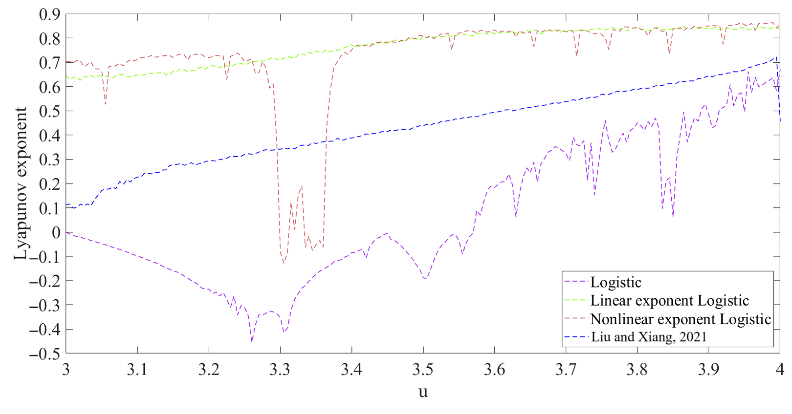
3.1. Maximum Lyapunov Exponent

The Lyapunov index is an important measure of chaotic maps, which represents the average exponential rate of convergence or divergence between adjacent orbits in phase space. The existence of at least one positive Lyapunov index in a map means that in the map phase space, no matter how small the initial spacing between the two tracks, the difference will increase exponentially over time, eventually reaching an unpredictable degree; that is, the map is chaotic. When the Lyapunov index is less than zero, it means that the adjacent points will eventually converge and merge into a point, becoming a stable fixed point, and the same orbit will enter periodic motion. In Figure 1, it can be seen that after adding the exponential part of the digital logistic map, the value of the Lyapunov exponent is in the range of (3, 4), and the same parameter is greater than the original digital logistic map, which not only indicates that the digital logistic map is still in a chaotic state in exponential mode, but also that its dynamic characteristics are more complex. Literature [22] by improving the original digital logistic map, the Lyapunov exponent tends to be 0.7 in the range [3, 4], which is lower than the linear exponential digital logistic map and lower than the nonlinear exponential digital logistic map in most ranges.

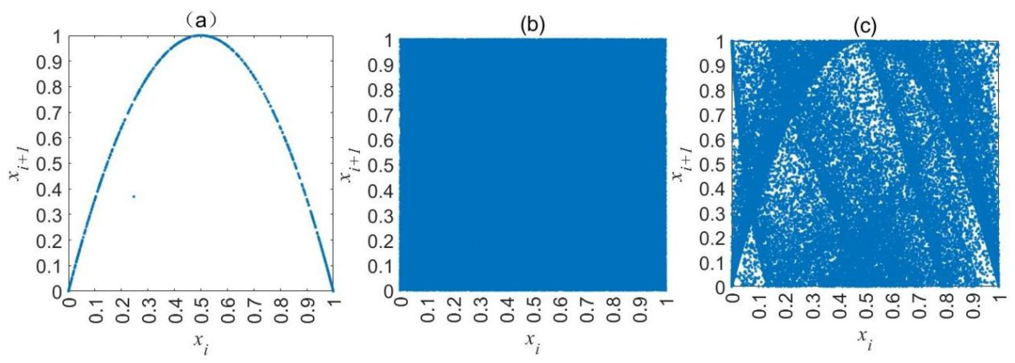
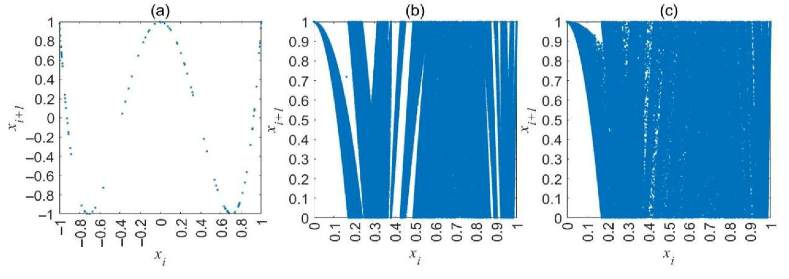
3.2. Trajectory and Phase Diagrams

In this test, the accuracy is set to 18 and represents retaining 18 decimal places. The motion trajectory of the original digital logistic map Equation (5), the motion trajectory under the linear exponential feedback Equation (7), and the motion trajectory under the nonlinear exponential feedback Equation (8) are shown in Figure 2a, b, and c, respectively. It can be seen from the figure that after 2000 iterations, the original digital logistic map has entered a loop when it is iterated less than 200 times, while the two maps after adding the exponential delay feedback method have no obvious tendency of periodic movement, let alone obvious structural features. This result shows that the exponential delay feedback method can effectively extend the number of iterations of the digital logistic map into the cycle. Figure 3 shows the distribution of the values generated by the three maps after 200,000 iterations in the [0, 1] space, and when the accuracy is finite, it can be seen that the original digital logistic map phase space approximates a quadratic function image and cannot traverse the space within (0, 1). For Figure 3b, the linear exponential digital logistic map can greatly improve its traversability, occupying all the space in (0, 1), but destroying the phase space structure of the original digital map. Compared with this, it can be solved in the nonlinear exponent. Compared with the original map in C, it not only improves its traversability but also shows that this method will not completely destroy the phase space structure of the original map. In order to reduce the dynamic degradation of the map as much as possible, the spatial structure of the original phase should be preserved as much as possible, which is an important criterion for reducing the dynamic degradation of the digital chaos map.

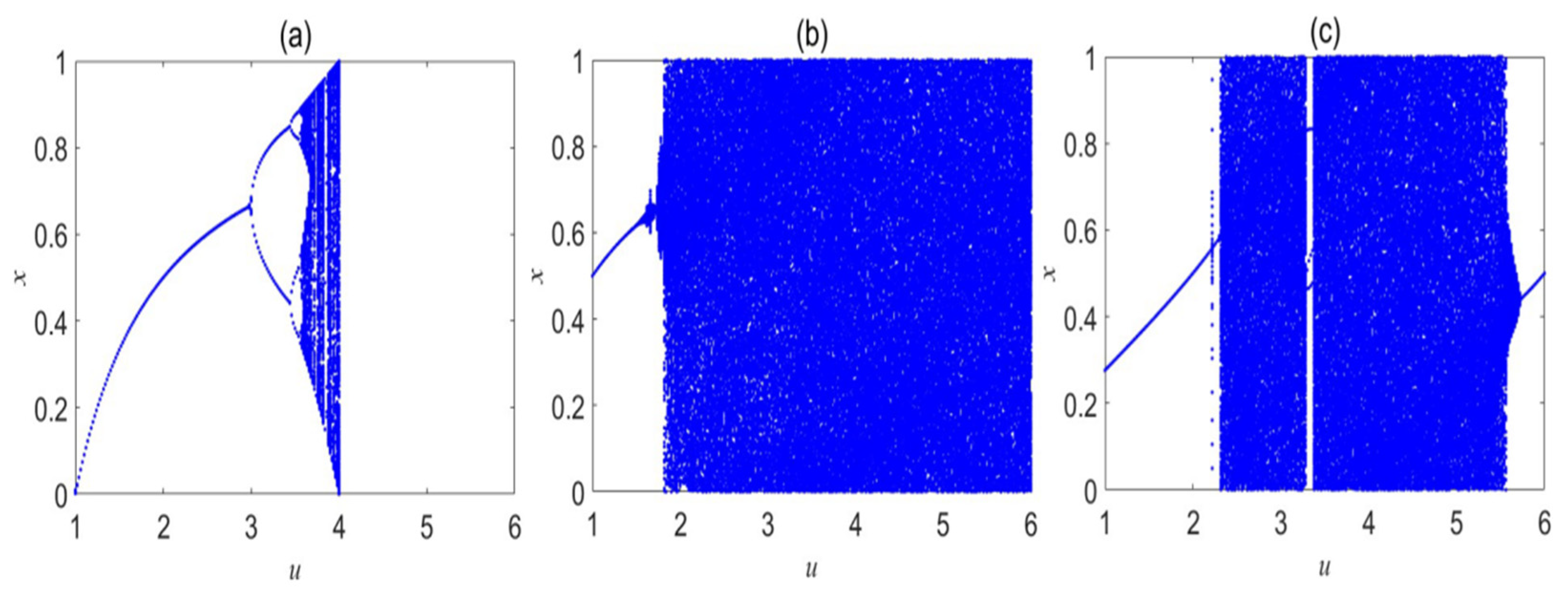
3.3. Bifurcation Diagram

Bifurcation refers to a small and continuous change in the control parameters of a digital chaos map, which leads to a change in the topology of the entire map; it can reveal the complexity and sensitivity of the system as parameters change. Ref. [7] Figure 4 shows the bifurcation of the three maps. The original digital logistic map can only reach the chaotic state when the control parameter value is (3.5699456, 4], as can be seen from the figure. In the linear exponential case, the control parameters are in the full map state in the range of (1.8, 6], which not only enlarges the value range of the control parameters but also reduces the period window of the original digital logistic map. In the nonlinear exponential case, a periodic window appears when the parameter u = 3.2, which indicates that the chaotic performance of the digital chaos map is poorer at this point, but the effect is also stronger than that of the original digital logistic map, and it has been experimentally verified that the bifurcation map forms a periodic motion when the control parameter a ≥ 6.

3.4. Period Analysis

The period is an important measure of the degradation of the dynamics of a digital chaotic map. Two main aspects are considered here: one is the number of iterations of the digital chaotic map entering the cycle for the first time, and the other is the length of the cycle, that is, the number of iterations elapsed between the first entry into the cycle and the second entry into the cycle. In this test, the length of the sequence is set to 2 × 10⁵. The parameters were kept constant, and the maximum accuracy was varied from $2^{-8}$ to $2^{-24}$. The length of entering a cycle and the number of iterations of the cycle are shown in

Table 1. Cycle analysis of the original, linear exponential, and nonlinear exponential digital logistic diagrams (1 means that all subsequent sequence values are 0, and N denotes undetected).

Precision	Period of Equation (5)	Period of Equation (7)	Period of Equation (8)	Number of Iterations When Entering a Cycle (Equation (5))	Number of Iterations When Entering a Cycle (Equation (7))	Number of Iterations When Entering a Cycle (Equation (8))
$2^{-8}$	4	1	98	20	194	63
$2^{-9}$	7	1	1	17	801	30
$2^{-10}$	3	200	362	22	1656	203
$2^{-11}$	6	329	1	13	1352	83
$2^{-12}$	9	5424	312	82	2730	305
$2^{-13}$	42	1	1032	15	2006	1839
$2^{-14}$	63	1	1013	82	3606	256
$2^{-15}$	91	1	32	47	6204	3513
$2^{-16}$	79	1	10,931	77	87,639	3357
$2^{-17}$	199	125,271	1	8	47,014	17,407
$2^{-18}$	588	N	1902	75	N	43,628
$2^{-19}$	656	1	6662	63	96,865	10,636
$2^{-20}$	451	N	33,071	52	N	19,982
$2^{-21}$	311	N	N	301	N	N
$2^{-22}$	931	N	N	596	N	N
$2^{-23}$	771	N	N	786	N	N
$2^{-24}$	993	N	N	1791	N	N

below, from which it can be seen that using the exponential feedback method with different precision can extend the cycle length and the number of iterations entering the first cycle is greatly increased. It can be concluded that this method is highly competitive with other methods in terms of extending the cycle. The number of iterations of the sequence when it first enters the cycle is often neglected in studies such as [23,24,25]. When comparing the numerical logistic map from

Table 2. Number of iterations when first entering a cycle.

Presicion	Equation (7)	Equation (8)	Ref. [24]	Ref. [25]
$2^{-8}$	194	63	11	15
$2^{-9}$	801	30	32	6
$2^{-10}$	1656	203	39	18
$2^{-11}$	1352	83	6	34
$2^{-12}$	2730	305	6	34
$2^{-13}$	2006	1839	81	48
$2^{-14}$	3606	256	6	29
$2^{-15}$	6204	3513	63	52

with other methods [24,25], we find that this feedback delay method can greatly improve the periodicity properties of the numerical logistic map, indicating that the method is effective.

3.5. Correlation Dimension Analysis

The correlation dimension is one of the correlation dimensions and is often used as a measure of the complexity of chaotic signals. We can use MATLAB R2022a’s own correlationDimension() function to calculate the correlation dimension of Equations (5), (7) and (8). The test results are shown in Figure 5. The correlation dimension of the original digital logistic map has been at a low level in the figure, and after adding the exponential delay feedback method, the correlation dimension increases greatly, although the parameter in the nonlinear exponential in the range (3.3, 3.35) remains at the same level as the original digital logistic map because of the period window but is still steadily higher than the original digital logistic map in general. The parameter is close to 3.5 when the linear exponential feedback method is used. There is a drop in the correlation dimension due to the autocorrelation of the sampling sequence, which proves that the complexity of the chaotic attractor also decreases rapidly at this point.

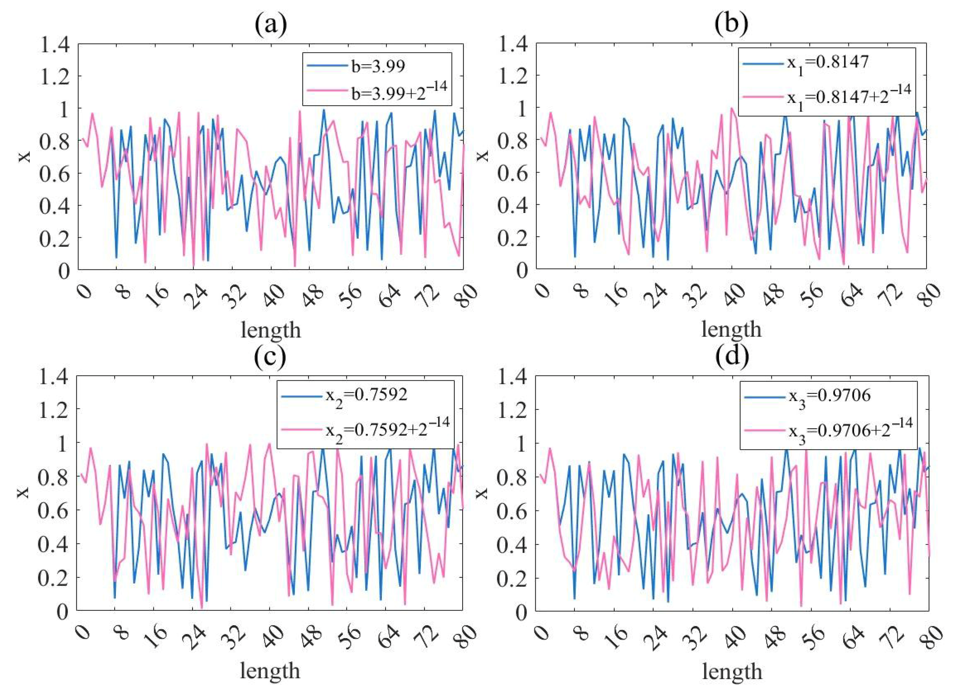
3.6. Sensitivity Analysis of Initial Condition

The sensitivity to the initial state and control parameters of a digital chaotic map can be thought of as the difference when small changes in the initial values and control parameters occur. In theory, the chaotic sequence generated by a good digital chaotic map should have a high sensitivity. In this test, we increased both the initial conditions and parameters by 2⁻¹⁴ in size, and the trajectories generated by the linear exponential feedback and nonlinear exponential feedback methods sequences are shown in Figure 6 and Figure 7. The trajectories in Figure 6a and Figure 7a,b show a clear separation of the sequence trajectories after several iterations with different initial conditions, which demonstrates that Equations (7) and (8) are quite sensitive to the initial conditions; similar conclusions can be drawn for Figure 6b,c and Figure 7c,d after small changes in the state variables. It is also verified that Equations (7) and (8) are also sensitive to the state variables.

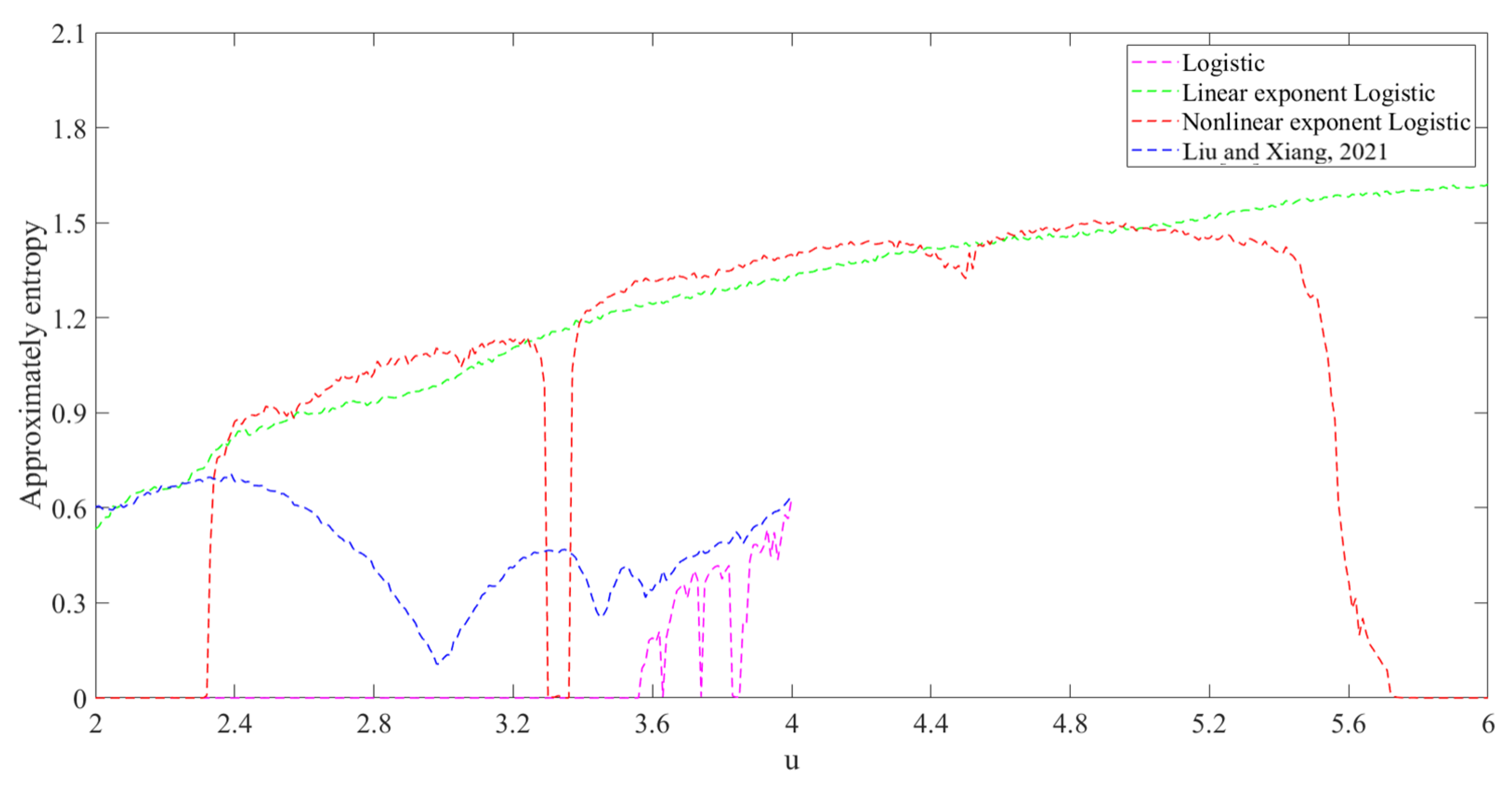
3.7. Approximate Entropy Analysis

Approximate entropy was first introduced in the literature [26]. If the approximate entropy of the sequence values generated by a chaotic map is greater than that of another chaotic map, it indicates that the chaotic map with a higher entropy value is more complex. In this test, the parameter u is set from 2 to 6, and the test results are shown in Figure 8. The figure shows that the chaotic interval of the original digital logistic map is at (3.56, 4], so the ApEn is at 0 until 3.56, and the chaotic property disappears after u = 4; the nonlinear exponential feedback method produces a sharp drop to 0 as the parameter u approaches 3.4 and 5.4 because of the period window, and the complexity of the generated sequence is lower at this point. Observe that the linear exponential feedback method remains greater than 0 from u = 1.8 onwards and increases as the parameters continue to increase. The exponential delay feedback method is more complex than the sequence generated by the original digital logistic map for the same parameters.

3.8. Permutation Entropy Analysis

The permutation entropy (PE) is also a measure of sequence complexity and was proposed in [27]. Measuring and comparing the original digital logistic map Equation (5) and the digital logistic map Equations (7) and (8) under the exponential delay feedback method, respectively. The horizontal coordinates were chosen as the independent variables, and the parameters were varied from 2 to 6 with the same accuracy in steps of 0.4. The results of this test are shown in Figure 9. From the figure, it can be seen that the PE of the improved model is greater than that of the original digital logistic map model under the same parameters. Equation (8) shows two decreases in PE due to the cycle window, and the improved model remains stable after u = 3.4, indicating that the improved model has some robustness to the parameters.

4. Exponential Feedback Digital Chebyshev Map Numerical Simulation

In this section, we continue to verify the feasibility of the method using the Chebyshev map as a pseudo-random sequence generator. The original Chebyshev map formula is as follows:

$$x_{i+1}=FL\circ \left(\mathit{cos}\right(b\times \mathit{arccos}{x}_i\left)\right).$$

(9)

In Equation (9), b is a parameter. From this, we can obtain the exponential control model under the exponential delay control method:

$$x_{i+1}=FL\circ \left(\left|\mathit{cos}{(b\times \mathit{arccos}{x}_i)}^{g\left(x_{i-k}\right)}\right|\mathit{mod}1\right).$$

(10)

Here we choose to control the pseudo-random sequence in the range (0, 1). Since the result of the sequence of the Chebyshev map will be negative, we have added absolute values to it so that the result also stays within (0, 1).

In Equation (10), when the exponential delay control function is a linear function, take g(x_i−k) = 1.09 − 0.59x_i−2. The inclusion of decimals complicates the calculations on the exponent and is used to resize the results of the exponential part.

$$x_{i+1}=FL\circ (4\cdot \left|0.5-\mathit{cos}{(b\times \mathit{arccos}{x}_i)}^{1.09-0.59x_{i-2}}\right|\mathit{mod}1).$$

(11)

Similarly, when the exponential delay control function is a nonlinear function, take g(x_i−k) = 1.09 − x_i−1x_i−2 and use x_i−1 instead of 0.59 not only to make g become a quadratic function form but also to change the complexity of the function, in which case we can get

$$x_{i+1}=FL\circ (4\cdot \left|0.5-\mathit{cos}{(b\times \mathit{arccos}{x}_i)}^{1.09-x_{i-1}\times x_{i-2}}\right|\mathit{mod}1).$$

(12)

In this test, to verify the effectiveness of the exponential delay feedback method for the digital Chebyshev map, we set the coefficients to ${p=18,b=3.99,x}_1=0.8147,x_2=0.7592$, k = 2, $x_3=0.9706$. In Equations (11) and (12), the values 4 and 0.5 are used to resize the function.

4.1. Trajectory and Phase Diagrams

Similar to the tests in the previous section, the accuracy is still set to 18, and the trajectories of the original digital Chebyshev map and the digital Chebyshev map with the addition of the exponential delay feedback method are shown in Figure 10a–c. It is obvious from Figure 10a that the digital Chebyshev map in the original state enters a cyclic state with more obvious structural features at less than 100 iterations, while the trajectory maps of the two improved digital Chebyshev maps are random and have no obvious structural features to detect their cycles up to 500 iterations. Figure 11 shows the phase space of the three digital Chebyshev maps, with the original state showing a trigonometric curve-like structure overall, while the latter two cases retain only the range of axes greater than 0 compared with the original range due to the addition of absolute values, which in this case improves the traversability compared with the original digital Chebyshev map while retaining some of the original phase space structure.

4.2. Period Analysis

Table 3. Period analysis of the original Chebyshev number map, linear exponential Chebyshev, and nonlinear exponential Chebyshev number map (N means not traversed).

Precision	Period of Equation (9)	Period of Equation (11)	Period of Equation (12)	Number of Iterations When Entering a Cycle (Equation (9))	Number of Iterations When Entering a Cycle (Equation (11))	Number of Iterations When Entering a Cycle (Equation (12))
$2^{-8}$	7	6	22	6	198	21
$2^{-9}$	7	342	244	26	381	26
$2^{-10}$	57	2490	80	7	403	95
$2^{-11}$	35	2107	59	13	1235	665
$2^{-12}$	28	257	864	9	7047	151
$2^{-13}$	40	20,734	2095	150	2532	3537
$2^{-14}$	134	19,359	4466	9	11,007	6205
$2^{-15}$	285	56,084	1960	34	19,559	10,172
$2^{-16}$	40	N	898	354	N	14,857
$2^{-17}$	196	N	9589	117	N	14,877
$2^{-18}$	30	N	70,591	66	N	89,621
$2^{-19}$	364	N	N	351	N	N
$2^{-20}$	1341	N	N	342	N	N
$2^{-21}$	1144	N	N	558	N	N
$2^{-22}$	528	N	N	36	N	N
$2^{-23}$	378	N	N	629	N	N
$2^{-24}$	1585	N	N	1353	N	N

shows a period analysis of the three different digit map methods regarding Chebyshev, with accuracy still ranging from $2^{-8}$ to $2^{-24}$. From the data in the table, it can be concluded that the period of the digital chaotic map is greatly extended compared with the original map at the same accuracy, and the number of iterations to enter the loop is greatly increased. With increasing upper limits of precision, both exponential number maps did not enter the loop for 200,000 iterations of the chaotic sequence after the precision reached $2^{-16}$ and $2^{-18},$ respectively. This shows that this method is more competitive with other methods in terms of cycle time extension.

4.3. Sensitivity Analysis

The linear delayed feedback Chebyshev digital chaos map should be extremely sensitive to the control and initial state variables, and in the tests in this subsection, both the control and initial state variables were varied by only $2^{-14}$, and then the generated trajectories were compared, with the results shown in Figure 12. The trajectories in Figure 12a show that under different control variables, the trajectories produce a significant separation in less than eight iterations, which proves that Equation (11) is quite sensitive to the control variables, and similar conclusions can be drawn for Figure 12b–d, which proves that Equation (11) is highly sensitive to the initial state variables. The results of the sensitivity test for Equation (12) are plotted in Figure 13, which shows that again the trajectory produces a significant separation at less than eight iterations, both demonstrating the high sensitivity of Equation (12) to the initial values and state variables.

4.4. Correlation Dimension Analysis

Figure 14 shows the correlation dimension analysis of Equations (9), (11) and (12). Here we take the first 50,000 data points of the generated sequence, and the results are shown in Figure 14. A comparison of the data in the figure reveals that the Chebyshev map with parameters in the range of [3, 4] after the linear delay feedback method has much larger values of the correlation dimension than the original numerical map, while the difference in the values under the two linear delays is small. When the parameter b > 3.95, the improved digital chaotic map correlation dimension value has a significant decay due to the presence of autocorrelation of the sampled sequences, so that the geometric complexity of its chaotic attractor is lower when the parameter value is within [3.95, 4].

4.5. Approximate Entropy Analysis

In this experiment, we calculated the ApEn of the sequences generated from Equations (9), (11) and (12) to compare the magnitude relationship between them; see Figure 15. It can be seen from the line data in the figure that the value of the approximate entropy of the improved Chebyshev map is considerably higher than compared with the original map, and the values of the improved map are relatively stable and do not have the large ups and downs fluctuations of the approximate entropy values of the original map. This indicates that the improved numerical map generates sequences of higher complexity and has a greater competitive advantage over other methods.

4.6. Permutation Entropy Analysis

Permutation entropy measures the uncertainty of the order based on the magnitude of the continuous value of the sequence given by the numerical chaotic map, with higher values of permutation entropy indicating greater robustness compared with other metrics. As can be seen from Figure 16, under the same parameter conditions, the PE values of both linear exponential and nonlinear exponential Chebyshev maps are greater than or equal to the PE values of the original state and remain relatively stable in the parameter range from 2 to 6, which suggests that the improved exponential numerical map is not only improved in complexity but also robust to parameter variations.

5. Application of Image Encryption Algorithm

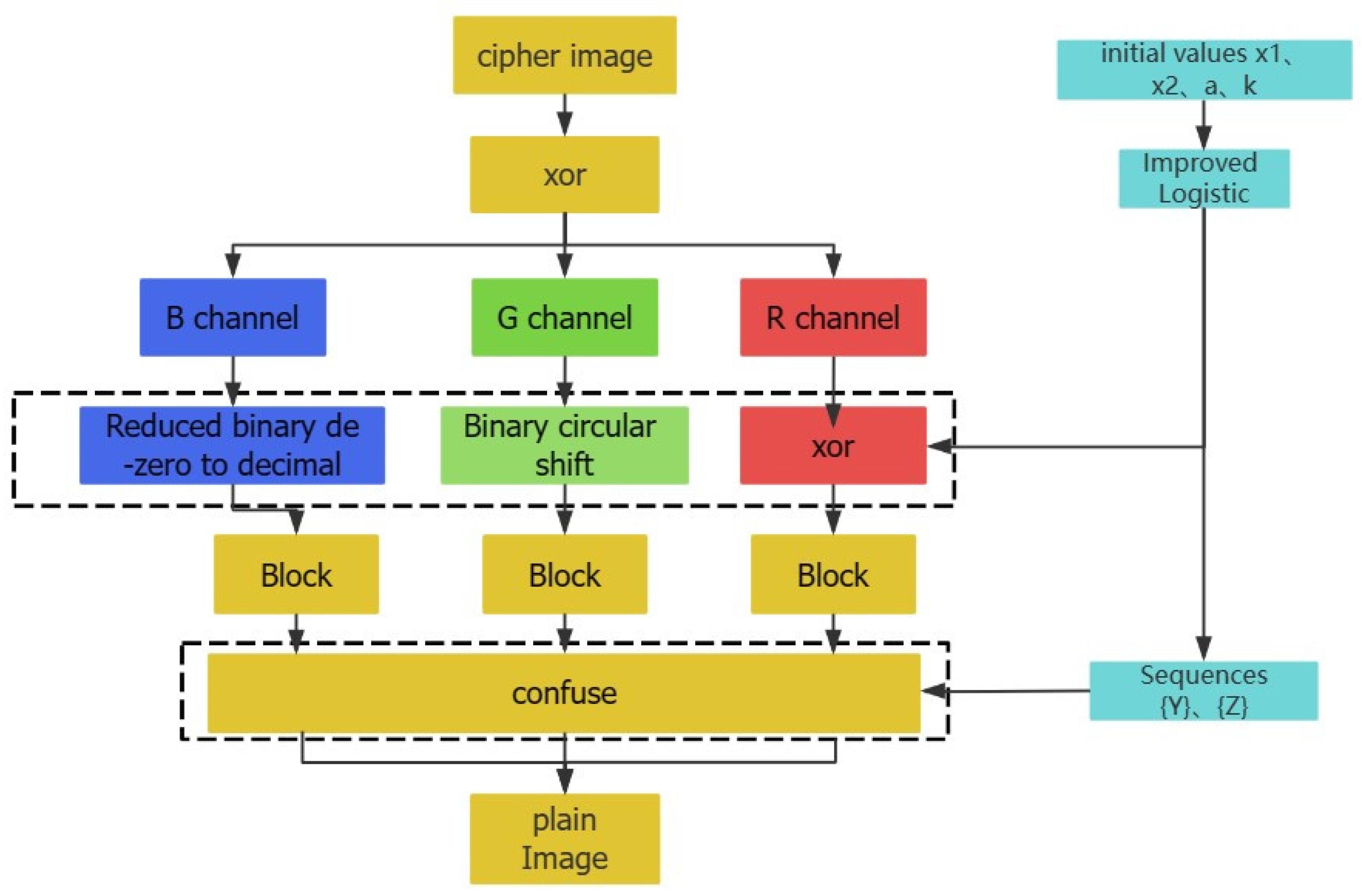
5.1. Image Encryption Algorithm Based on Linear Exponential Delayed Feedback Logstic

In Section 3, the proposed linear exponential delayed feedback Logistic chaos model with good dynamic properties is analyzed theoretically and numerically and effectively reduces the dynamics degradation in the case of finite accuracy. Moreover, the linear exponential delay feedback Logistic map has more stable performance and lower implementation complexity compared with the nonlinear one, which has wide applicability. This section uses a simple cryptographic algorithm to illustrate the validity and applicability of the linear exponential Logistic chaos model. The algorithm is simpler to operate, and the security relies on the chaotic model itself, which is shown through the following experiments to be highly secure and resistant to attack when applied to image encryption applications. The color image size used in this application is M × N, and this encryption algorithm describes the process as follows.

Step 1: Enter the initial values $x_1$, $x_2$, $k$, as the key where $x_1$ is the mean value mod 1 of the image pixels, $x_2$ is the variance of the pixel values in each row of the image pixels, and the variance and mod 1 of the pixel values in each column.

Step 2: Divide the image into three channels R, G, and B.

Step 3: The image is chunked and processed for the sequence {X} generated by the digital chaos map. The sequence {Y} consists of a sequence of even subscripts starting from 2. Thus,${\left\{Y\right\}=\{x}_2,x_4,x_6,\dots \dots x_{(M/2)\times (N/2)}\}$, the sequence ${\left\{Z\right\}=\{x}_{20000},x_{20001},......x_{M\times N+19999}\}$, and the sequence {Z} discards the first 20,000 values.

Step 4: Sort {Y} and {Z} in ascending order and keep the index constant. The index sequence of sequence {Y} is used to disrupt each piece; after that, the chunked images are synthesized, and then the index sequence of sequence {Z} is used to disrupt them, and the three-channel synthesis yields the dislocated image.

Step 5: The obtained confusion image is divided into three channels with different diffusion methods. The R channel takes the pixel values and normalizes them with the chaotic sequence XOR. The G channel converts all pixel values to binary for splicing, after which it loops right-shifted by four bits and splits every eight bits to convert to decimal to get the new pixel value. The B channel converts the pixel value to decimal after adding 0 in the middle position so that it forms a nine-digit number, converts the decimal splice every three digits, uses the mod function Equation (13) to limit the data, and finally XORs to get the new pixel value.

$$W=\mathrm{mod}(floor(w)\times {10}^{15}), 256)$$

(13)

Step 6: The new three-channel synthesis yields encrypted images.

The flowchart of the encryption algorithm described above is shown in Figure 17 below, and the decryption process is the opposite of the encryption process. The decryption algorithm flowchart is shown below in Figure 18.

5.2. Security Analysis

5.2.1. Encryption and Decryption Analysis

In this section, four color images of size 256 × 256 are chosen as examples to verify the effectiveness of the encryption algorithm and that the encrypted images can be decrypted accurately when the correct key is used. The results of Figure 19 show that the algorithm is able to perform the encryption and decryption operations accurately. Figure 19a–d is encrypted to get the ciphertext image Figure 19e–h and then decrypted using the correct key to get Figure 19i–l.

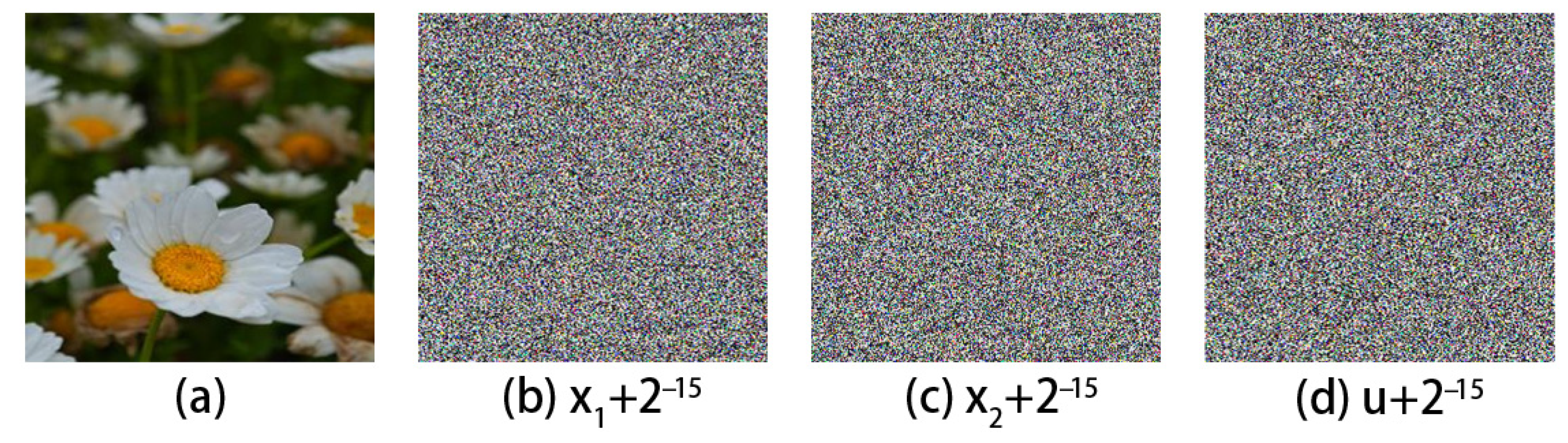
5.2.2. Key Sensitivity Analysis

Key sensitivity is a characteristic that measures the difference between encrypted and decrypted images. A good encryption algorithm should be highly sensitive to the key, which means that any small change in the key will prevent the image from being successfully decrypted. Figure 20 shows the decrypted images with keys u, $x_1$, and $x_2$ producing 2⁻¹⁵ differences, respectively, and the results show that the decrypted images are noisy and unrecognizable, indicating that the present algorithm is highly sensitive to the keys.

5.2.3. Key Space Analysis

A secure image encryption algorithm should have a key space greater than 2¹²⁸ used to resist brute force attacks. In this encryption scheme, there are four parameters that can be adjusted for the parameters u and k, as well as the mean variance mod1 originating from the image itself, as the initial values $x_1,x_2.$ Assuming a maximum computational accuracy of 10^−r and setting r to 14 for the purpose of comparison with other encryption schemes, the key space of this encryption algorithm is 10⁵⁶, which is approximately equal to 2¹⁸⁶, a result much larger than 2¹²⁸, indicating that the key space is resistant to brute force attacks. The results for key spaces larger than [28,29,30,31,32] under the same computational accuracy conditions are shown in

Table 4. Key space.

Algorithm	Key Space
Proposed	2186
Ref. [28]	2176
Ref. [29]	2160
Ref. [30]	2139
Ref. [31]	2186
Ref. [32]	2186

.

5.2.4. Histogram Analysis

A histogram shows the information about the distribution of pixels in an image. The histogram of a secure image should be flat and even, making it impossible for an external attacker to get any information about the image from the histogram of the image. Figure 21 represents the distribution of pixel values, where Figure 21a–d shows the histogram of the original image and Figure 21e–h represents the histogram of the image after correct encryption. It can be seen that there are peaks before encryption, and then after going through the encryption, the peaks become flat and uniform, which is significantly different from the histogram of the original image, and it is difficult for the attacker to obtain the information of the image in this uniform situation.

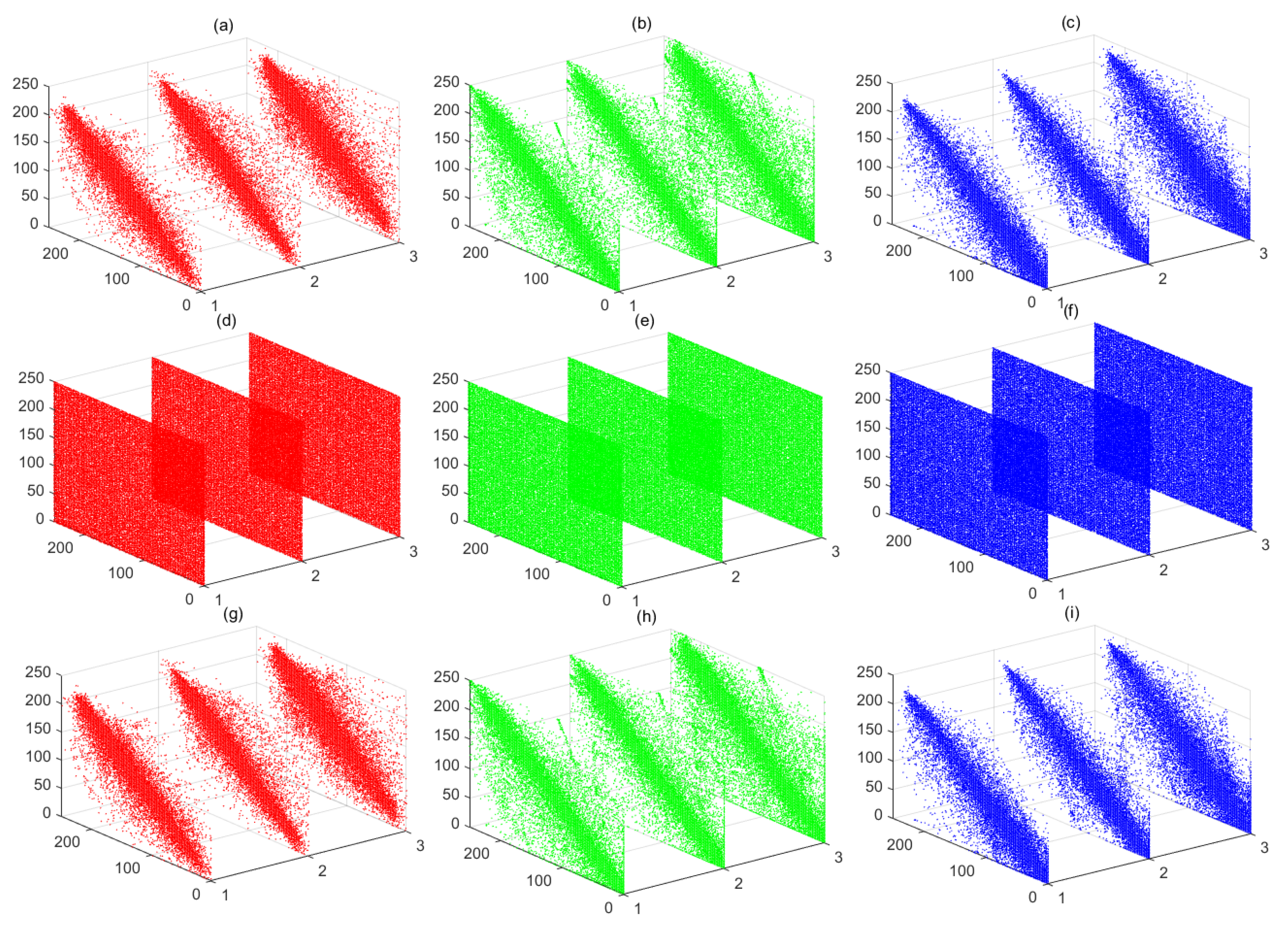
5.2.5. Pixel Correlation Analysis

For plaintext images, the pixel correlation between two adjacent points is often very high, and an effective encryption scheme is to break this correlation. In this test, the R, G, and B channels of the plaintext image and the ciphertext image of peppers are experimented with in horizontal, vertical, and diagonal directions, and the results are shown in Figure 22. Red represents the R component, green represents the G component, and blue represents the B component, and the graph shows horizontal, vertical, and diagonal correlations from left to right. From the figure, it can be seen that the neighboring pixels in each different direction of the three channels of the plaintext image are mainly clustered along the diagonal, while the neighboring pixels of the encrypted image after the encryption scheme are randomly tiled throughout the space, which indicates that the present encryption scheme has completely weakened the correlation between the neighboring pixels. The correlation coefficient can also be calculated to measure the resistance of this algorithm against correlation attacks. The correlation coefficient is calculated as in Equation (14).

$$R={{\displaystyle \frac{\underset{i=1}{\overset{N}{{\displaystyle \Sigma }}}\left(\right(x_i-\frac{1}{N}\underset{i=1}{\overset{N}{{\displaystyle \Sigma }}}{x}_i)\times (y_i-\frac{1}{N}\underset{i=1}{\overset{N}{{\displaystyle \Sigma }}}{y}_i\left)\right)}{\sqrt{\underset{i=1}{\overset{N}{{\displaystyle \Sigma }}}{{\displaystyle \left(\right(x_i-\frac{1}{N}\underset{i=1}{\overset{N}{{\displaystyle \Sigma }}}{x}_i\left)\right)}}^2}\times \sqrt{\underset{i=1}{\overset{N}{{\displaystyle \Sigma }}}{{\displaystyle \left(\right(y_i-\frac{1}{N}\underset{i=1}{\overset{N}{{\displaystyle \Sigma }}}{y}_i\left)\right)}}^2}}}}_{.}$$

(14)

where R is the correlation coefficient, N is the length of the test sequence, and x and y are the pixel values of a pair of random neighboring pixels. Usually, the correlation coefficient of the original image is close to 1, and there is a strong correlation between the neighboring pixels after the encryption scheme to make its value close to 0, in order to prove that this algorithm has some superiority and competitiveness.

Table 5. Correlation coefficient analysis.

Image	Derection	Cipher Image
		R	G	B
Flowers	Horizontal	0.0020	0.0015	−0.0017
	Vertical	−0.0016	0.0031	−0.0020
	Diagonal	0.0017	−0.0021	−0.0025
Boats	Horizontal	0.0013	0.0029	−0.0029
	Vertical	0.0031	0.0022	−0.0032
	Diagonal	0.0021	−0.0019	−0.0011
Gorilla	Horizontal	0.0019	−0.0025	0.0022
	Vertical	0.0023	−0.0035	−0.0011
	Diagonal	−0.0039	−0.0027	0.0014
Peppers	Horizontal	−0.0013	0.0014	0.0019
	Vertical	0.0015	0.0024	−0.0023
	Diagonal	−0.0018	0.0016	0.0044
Ref. [33]	Horizontal	−0.004	−0.0042	−0.0009
	Vertical	−0.0007	0.0012	−0.0069
	Diagonal	−0.0019	0.0021	−0.0041
Ref. [34]	Horizontal	−0.0104	0.0180	0.0087
	Vertical	0.0178	0.0006	−0.0063
	Diagonal	−0.0049	−0.000015	0.0003

shows the correlation coefficients of Peppers before and after encryption, and the correlation coefficients of any component after encryption are close to 0 in all directions, indicating that our encryption scheme is effective. It is also highly competitive in comparison with the schemes presented in [33,34].

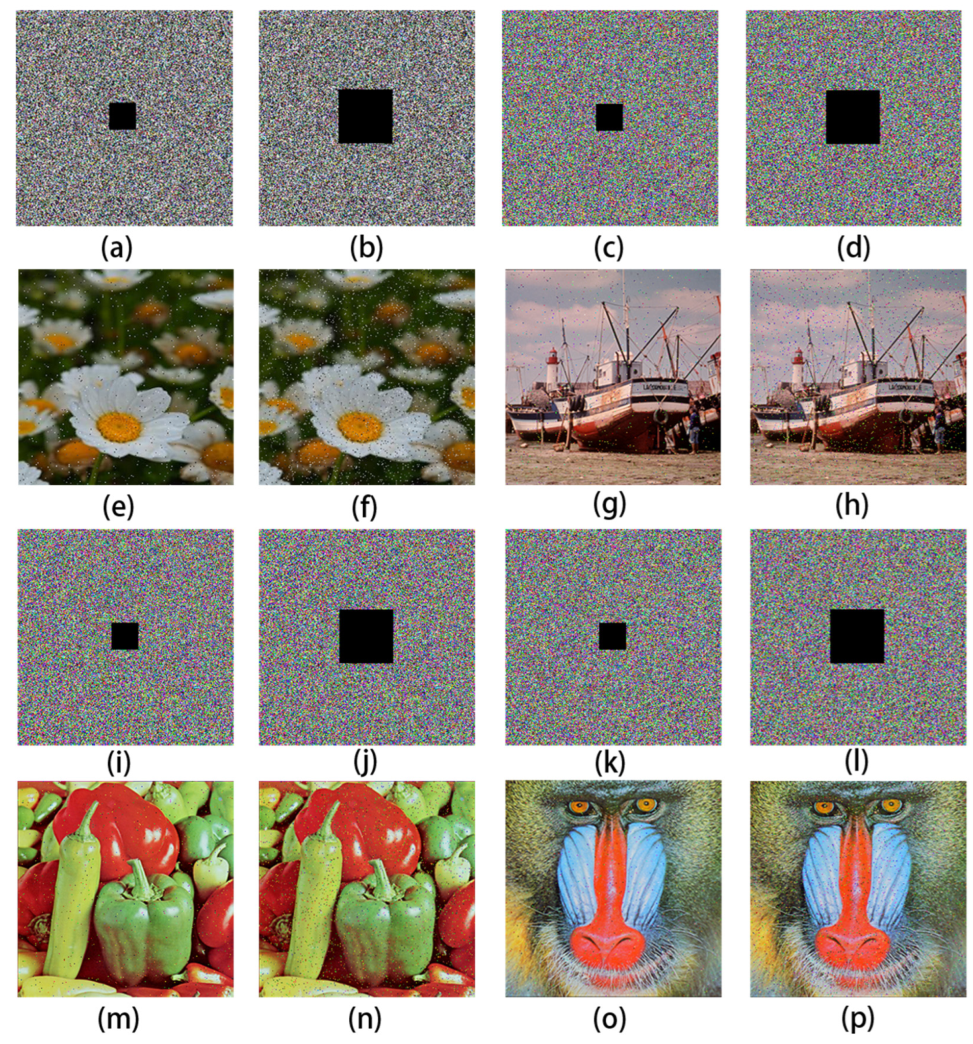
5.2.6. Robustness Analysis

Images are inevitably affected by noise or partial data loss during channel transmission, and a good encryption scheme should have the ability to resist such effects. The experimental results in Figure 23 and Figure 24 demonstrate the performance of the algorithm. In this experiment, by adding 1% and 5% pretzel noise or 32 × 32 and 64 × 64 shear attack cases, we can still get the correct decrypted image, which shows that the scheme has good robustness.

5.2.7. Resistance to Differential Attacks

Differential attack is a common attack to exploit the correlation of the image to compromise the algorithm. A secure and sensitive algorithm should be such that when the pixels of the plaintext image undergo a small change, the corresponding encrypted image is supposed to be very different from the one before the pixels do not change. The pixel change rate (NPCR) as well as the average intensity of the change (UACI) are usually used to measure the sensitivity of the encryption algorithm to the plaintext image, which is computed as (15) and (16)

$$NPCR={\displaystyle \frac{\underset{i}{\overset{M}{{\displaystyle \Sigma }}}\underset{j}{\overset{N}{{\displaystyle \Sigma }}}G(i,j)}{M\times N}}\times 100\%$$

(15)

$$UACI={\displaystyle \frac{\underset{i}{\overset{M}{{\displaystyle \Sigma }}}\underset{j}{\overset{N}{{\displaystyle \Sigma }}}\left|P(i,j)-P^{\prime }(i,j)\right|}{M\times N\times 255}}\times 100\%$$

(16)

where M and N are the number of rows as well as the number of columns of the image, respectively, and the value of G(i,j) is 1 when the pixel at a point changes and 0 otherwise. $p_{(i,j)}$ and $p_{(i,j)}^{\prime }$ are the pixel values before and after the image change. In the ideal case, the values of NPCR and UACI should be 0.9961 and 0.3346. In our testing scheme, the ciphertext image is tested separately in separate channels, and the results obtained by randomly changing one pixel are shown in

Table 6. Values of NPCR and UACI.

Images	Channel	NPCR	UACI
Flowers	R	0.9962	0.3350
	G	0.9961	0.3344
	B	0.9961	0.3345
Boats	R	0.9960	0.3345
	G	0.9959	0.3340
	B	0.9960	0.3345
Gorilla	R	0.9961	0.3345
	G	0.9959	0.3344
	B	0.9960	0.3344
Peppers	R	0.9960	0.3350
	G	0.9962	0.3343
	B	0.9963	0.3346
Ref. [34]	R	0.9959	0.3355
	G	0.9961	0.3335
	B	0.9961	0.3343
Ref. [35]	R	0.9960	0.3335
	G	0.9960	0.3347
	B	0.9938	0.3344

. From the data in the table, it can be concluded that both of them are closer to the ideal value, and hence their performance against differential attacks is superior and also competitive as compared with [34,35].

6. Conclusions

When digital chaotic maps were used on devices with limited precision, dynamic degradation occurred, resulting in features that were no longer applicable in encryption. Therefore, this paper proposed a method based on exponential delayed feedback to reduce the dynamic degradation of digital chaotic maps, using the improved linear and nonlinear one-dimensional Logistic map and Chebyshev map as examples. Numerical simulations were conducted for experiments on trajectories, phase space, correlation dimensions, sensitivity to initial conditions, bifurcation maps, Lyapunov exponents, periods, ApEn, and PE. The experimental results showed that the method was effective in resisting dynamic degradation. Additionally, we designed a cryptographic algorithm using a linear exponential Logistic map to demonstrate the method’s practicality. Analyses of histograms, robustness, and resistance to differential attacks demonstrated that the encryption algorithm was highly secure, had the ability to resist various external attacks, and was competitive with other encryption schemes. The exponential delay feedback method would be further improved in subsequent scientific research and combined with other cryptographic schemes to enhance its applicability in cryptography.

References

1. Alexan, W.; Elkandoz, M.; Mashaly, M.; Azab, E.; Aboshousha, A. Color image encryption through chaos and KAA map. IEEE Access 2023, 11, 11541–11554. [Google Scholar] [CrossRef]
2. ErkErkan, U.; Toktas, A.; Lai, Q. 2D hyperchaotic system based on Schaffer function for image encryption. Expert Syst. Appl. 2022, 213, 119076. [Google Scholar] [CrossRef]
3. Li, S.; Chen, G.; Mou, X. On the dynamical degradation of digital piecewise linear chaotic maps. Int. J. Bifurc. Chaos 2005, 15, 3119–3151. [Google Scholar] [CrossRef]
4. Liu, L.; Wang, J. A shift coupling digital chaotic model with counteracting dynamical degradation. Nonlinear Dyn. 2023, 111, 19459–19486. [Google Scholar] [CrossRef]
5. Xiang, H.; Liu, L. An improved digital logistic map and its application in image encryption. Multimed. Tools Appl. 2020, 79, 30329–30355. [Google Scholar] [CrossRef]
6. Wu, Y.; Liu, L.; Giesl, P. An iteration-time combination method to reduce the dynamic degradation of digital chaotic maps. Complexity 2020, 2020, 5707983. [Google Scholar] [CrossRef]
7. Zhao, Y.; Xu, C.; Xu, Y.; Lin, J.; Pang, Y.; Liu, Z.; Shen, J. Mathematical exploration on control of bifurcation for a 3D predator-prey model with delay. AIMS Math. 2024, 9, 29883–29915. [Google Scholar] [CrossRef]
8. Wang, J.; Liu, L. A novel chaos-based image encryption using magic square scrambling and octree diffusing. Mathematics 2022, 10, 457. [Google Scholar] [CrossRef]
9. Iskakova, K.; Alam, M.M.; Ahmad, S.; Saifullah, S.; Akgül, A.; Yılmaz, G. Dynamical study of a novel 4D hyperchaotic system: An integer and fractional order analysis. Math. Comput. Simul. 2023, 208, 219–245. [Google Scholar] [CrossRef]
10. Zhu, Y.; Wang, C.; Sun, J.; Yu, F. A chaotic image encryption method based on the artificial fish swarms algorithm and the DNA coding. Mathematics 2023, 11, 767. [Google Scholar] [CrossRef]
11. Huang, X.; Dong, Y.; Ye, G.; Shi, Y. Meaningful image encryption algorithm based on compressive sensing and integer wavelet transform. Front. Comput. Sci. 2023, 17, 173804. [Google Scholar] [CrossRef]
12. Zhu, S.; Deng, X.; Zhang, W.; Zhu, C. Image encryption scheme based on newly designed chaotic map and parallel DNA coding. Mathematics 2023, 11, 231. [Google Scholar] [CrossRef]
13. Zhao, H.; Gong, Z.; Gan, K.; Gan, Y.; Xing, H.; Wang, S. Supervised kernel principal component analysis-polynomial chaos-Kriging for high-dimensional surrogate modelling and optimization. Knowl.-Based Syst. 2024, 305, 112617. [Google Scholar] [CrossRef]
14. Chen, Y.; Li, H.; Song, Y.; Zhu, X. Recoding hybrid stochastic numbers for preventing bit width accumulation and fault tolerance. IEEE Trans. Circuits Syst. I Regul. Pap. 2024, 72, 1243–1255. [Google Scholar] [CrossRef]
15. Yang, J.; Liu, Z.; Wang, G.; Zhang, Q.; Xia, S.; Wu, D.; Liu, Y. Constructing three-way decision with fuzzy granular-ball rough sets based on uncertainty invariance. IEEE Trans. Fuzzy Syst. 2025, 33, 1781–1792. [Google Scholar] [CrossRef]
16. Khan, J.S.; Ahmad, J. Chaos based efficient selective image encryption. Multidimens. Syst. Signal Process. 2019, 30, 943–961. [Google Scholar] [CrossRef]
17. Zhu, H.; Dai, L.; Liu, Y.; Wu, L. A three-dimensional bit-level image encryption algorithm with Rubik’s cube method. Math. Comput. Simul. 2021, 185, 754–770. [Google Scholar] [CrossRef]
18. Liu, L.; Xiang, H.; Li, X. A novel perturbation method to reduce the dynamical degradation of digital chaotic maps. Nonlinear Dyn. 2021, 103, 1099–1115. [Google Scholar] [CrossRef]
19. Ren, Q.; Teng, L.; Jiang, D.; Si, R.; Wang, X. Visual image encryption algorithm based on compressed sensing and 2D cosine-type logistic map. Phys. Scr. 2023, 98, 095212. [Google Scholar] [CrossRef]
20. Shukla, V.K.; Joshi, M.C.; Mishra, P.K.; Xu, C. Mechanical analysis and function matrix projective synchronization of El-Nino chaotic system. Phys. Scr. 2024, 100, 015255. [Google Scholar] [CrossRef]
21. Shukla, V.K.; Joshi, M.C.; Mishra, P.K.; Xu, C. Adaptive fixed-time difference synchronization for different classes of chaotic dynamical systems. Phys. Scr. 2024, 99, 095264. [Google Scholar] [CrossRef]
22. Han, C. An image encryption algorithm based on modified logistic chaotic map. Optik 2019, 181, 779–785. [Google Scholar] [CrossRef]
23. Liu, L.; Liu, B.; Hu, H.; Miao, S. Reducing the dynamical degradation by bi-coupling digital chaotic maps. IntInt. J. Bifurc. Chaos 2018, 28, 1850059. [Google Scholar] [CrossRef]
24. Liu, L.; Miao, S. Delay-introducing method to improve the dynamical degradation of a digital chaotic map. Inf. Sci. 2017, 396, 1–13. [Google Scholar] [CrossRef]
25. Liu, J.; Liang, Z.; Luo, Y.; Cao, L.; Zhang, S.; Wang, Y.; Yang, S. A hardware pseudo-random number generator using stochastic computing and logistic map. Micromachines 2020, 12, 31. [Google Scholar] [CrossRef]
26. Pincus, S.M. Approximate entropy as a measure of system complexity. Proc. Natl. Acad. Sci. USA 1991, 88, 2297–2301. [Google Scholar] [CrossRef]
27. Bandt, C.; Pompe, B. Permutation entropy: A natural complexity measure for time series. Phys. Rev. Lett. 2002, 88, 174102. [Google Scholar] [CrossRef]
28. Xiang, H.; Liu, L. A new perturbation-feedback hybrid control method for reducing the dynamic degradation of digital chaotic systems and its application in image encryption. Multimed. Tools Appl. 2021, 80, 19237–19261. [Google Scholar] [CrossRef]
29. Zhang, Y.; Xu, B.; Zhou, N. A novel image compression—Encryption hybrid algorithm based on the analysis sparse representation. Opt. Commun. 2017, 392, 223–233. [Google Scholar] [CrossRef]
30. Chen, C.; Sun, K.H.; Peng, Y.X.; Alamodi, A. A novel control method to counteract the dynamical degradation of a digital chaotic sequence. Eur. Phys. J. Plus 2019, 134, 31. [Google Scholar] [CrossRef]
31. Liu, Y.; Qin, Z.; Liao, X.; Wu, J. Cryptanalysis and enhancement of an image encryption scheme based on a 1-D coupled Sine map. Nonlinear Dyn. 2020, 100, 2917–2931. [Google Scholar] [CrossRef]
32. Zhang, Y.-Q.; Huang, H.-F.; Wang, X.-Y.; Huang, X.-H. A secure image encryption scheme based on genetic mutation and MLNCML chaotic system. Multimed. Tools Appl. 2021, 80, 19291–19305. [Google Scholar] [CrossRef]
33. Jithin, K.; Sankar, S. Colour image encryption algorithm combining Arnold map, DNA sequence operation, and a Mandelbrot set. J. Inf. Secur. Appl. 2020, 50, 102428. [Google Scholar] [CrossRef]
34. Xu, J.; Zhao, B.; Wu, Z. Research on color image encryption algorithm based on bit-plane and Chen Chaotic System. Entropy 2022, 24, 186. [Google Scholar] [CrossRef]
35. Alexan, W.; ElBeltagy, M.; Aboshousha, A. RGB image encryption through cellular automata, S-box and the Lorenz system. Symmetry 2022, 14, 443. [Google Scholar] [CrossRef]
Figure 1. Maximum LE comparison diagram with Ref. [18].
Mathematics 13 02324 g001
Figure 2. Trajectories analysis of the digital logistic maps. (a) Original digital logistic map; (b) Linear exponential digital logistic map; (c) Nonlinear exponential digital logistic map.
Mathematics 13 02324 g002
Figure 3. Phase space analysis of the digital logistic maps. (a) Original digital logistic map; (b) Linear exponential digital logistic map; (c) Nonlinear exponential digital logistic map.
Mathematics 13 02324 g003
Figure 4. Bifurcation comparison chart. (a) original digital logistic map; (b) linear exponential digital logistic map; (c) nonlinear exponential digital logistic map.
Mathematics 13 02324 g004
Figure 5. Comparison of the relevant correlation dimensions with Ref. [18].
Mathematics 13 02324 g005
Figure 6. Sensitivity of Equation (7): (a) initial value u ; (b) parameter x 1 ; (c) parameter x 2 .
Mathematics 13 02324 g006
Figure 7. Sensitivity of Equation (8): (a) initial value u; (b) initial value b; (c) parameter x 1 ; (d) parameter x 2 .
Mathematics 13 02324 g007
Figure 8. Analysis of the ApEn value under parameter variations with Ref. [18].
Mathematics 13 02324 g008
Figure 9. Analysis of the PE value under parameter variations with Ref. [18].
Mathematics 13 02324 g009
Figure 10. Trajectory analysis: (a) Raw Chebyshev number map; (b) Linear exponential Chebyshev number map; (c) Nonlinear exponential Chebyshev number map.
Mathematics 13 02324 g010
Figure 11. Phase space analysis (a) Primitive Chebyshev number map; (b) Linear exponential Chebyshev number map; (c) Nonlinear exponential Chebyshev number map.
Mathematics 13 02324 g011
Figure 12. Sensitivity of Equation (11): (a) initial value b; (b) parameter x 1 ; (c) parameter x 2 ; (d) parameter x 3 .
Mathematics 13 02324 g012
Figure 13. Sensitivity of Equation (12): (a) initial value b; (b) parameter x 1 ; (c) parameter x 2 ; (d) parameter x 3 .
Mathematics 13 02324 g013
Figure 14. Comparison of relevance dimensions of Equations (9), (11) and (12).
Mathematics 13 02324 g014
Figure 15. Comparison of approximate entropy analysis of Equations (9), (11) and (12) with different parameters.
Mathematics 13 02324 g015
Figure 16. Comparison of arrangement entropy analysis for Equations (9), (11) and (12) with different parameters.
Mathematics 13 02324 g016
Figure 17. Flowchart of encryption algorithm.
Mathematics 13 02324 g017
Figure 18. Decryption algorithm flowchart.
Mathematics 13 02324 g018
Figure 19. Encryption and decryption analysis: (ad) are the four original images, (eh) are the encryption result graphs, and (il) are the correct decryption result graphs.
Mathematics 13 02324 g019
Figure 20. Key sensitivity analysis: (a) Correct key decrypted image. (bd) Decrypted images with key producing 2−15 differences.
Mathematics 13 02324 g020
Figure 21. Statistical histogram: (ad) original image; (eh) encrypted image.
Mathematics 13 02324 g021
Figure 22. Pixel correlation analysis (ac) shows the R, G, B three-channel correlation of the original peppers image horizontally, vertically, and diagonally, respectively; (df) shows the correlation of the encrypted image; and (gi) shows the correlation of the decrypted image.
Mathematics 13 02324 g022
Figure 23. Robustness analysis: (ad) and (il) are the encrypted images after cutting 32 × 32 pixels and 64 × 64 pixels, respectively, (eh) and (mp) are their corresponding decrypted images.
Mathematics 13 02324 g023
Figure 24. Robustness analysis (ad) shows the decrypted image after adding 1% of pretzel noise, and (eh) shows the decrypted image after adding 5% of pretzel noise.
Mathematics 13 02324 g024