Quantifying the Complexity of Rough Surfaces Using Multiscale Entropy: The Critical Role of Binning in Controlling Amplitude Effects

Abstract

A salient feature of modern material surfaces used in cutting-edge technologies is their structural and spatial complexity, which endows them with novel properties and multifunctionality. The quantitative characterization of material complexity is a challenge that must be addressed to optimize their production and performance. While numerous metrics exist to quantify the complexity of spatial structures in various scientific domains, methods specifically tailored for characterizing the spatial complexity of material surface morphologies at the micro- and nanoscale are relatively scarce. In this paper, we utilize the concept of multiscale entropy to quantify the complexity of surface morphologies of rough surfaces across different scales and investigate the effects of amplitude fluctuations (i.e., surface height distribution) in both stepwise and smooth self-affine rough surfaces. The crucial role of the binning scheme in regulating amplitude effects on entropy and complexity measurements is highlighted and explained. Furthermore, by selecting an appropriate binning strategy, we analyze the impact of 2D imaging on the complexity of a rough surface and demonstrate that imaging can artificially introduce peaks in the relationship between complexity and surface amplitude. The results demonstrate that entropy-based spatial complexity effectively captures the scale-dependent heterogeneity of stepwise rough surfaces, providing valuable insights into their structural properties.

1. Introduction

The utilization of materials possessing surfaces with complex micro- and nanostructures has become increasingly significant in various scientific and industrial applications due to the diverse functions and properties they exhibit [1,2,3]. Images captured using techniques such as Scanning Electron Microscopy (SEM) [4,5] offer insights into these intricate structures by projecting the three-dimensional topography onto a two-dimensional plane, revealing vital aspects of surface morphology and spatial complexity. Surface morphology profoundly influences nanoscale applications, spanning material science to biotechnology, and, traditionally, it has been characterized using a plethora of roughness parameters such as root-mean-square (RMS) height, correlation length, and fractal dimension to name just a few [1,6,7,8,9,10]. Nevertheless, there is a growing consensus that a more comprehensive analysis may be necessary to fully capture the intricate behavior of these real-world topographies as the conventional metrics alone may not encompass the full complexity of the underlying surface structure [11].

Recent studies have introduced complexity metrics [12,13,14,15,16,17,18,19,20,21,22,23,24,25,26,27,28] as an alternative or complementary approach to the traditional roughness parameters. These complexity metrics, grounded in concepts such as Shannon entropy [29,30,31,32], have shown promise in characterizing synthetic and experimental surfaces alike. To date, however, their application has largely been explored only in relation to correlation length [13]. A gap remains in understanding how complexity metrics behave with respect to other critical roughness parameters, particularly RMS. RMS quantifies fluctuations in surface amplitudes and determines the width of their distribution. As RMS varies, the histogram range adjusts accordingly. Since calculations of Shannon entropy and the related entropy-based complexity depend on measuring histogram uniformity [33], the choice of a binning scheme [34] becomes a key issue when assessing the complexity of surfaces with differing RMS values and, therefore, histogram ranges.

Although entropy driven descriptors have shown promise, the literature still lacks a systematic assessment of how alternative histogram binning strategies influence entropy and, therefore, complexity across the complete range of RMS amplitudes. Prior studies usually lock the bin structure or focus only on correlation length, leaving unresolved how amplitude scaling biases complexity estimates and how those estimates translate from raw height maps to their corresponding image representations.

In this paper, we systematically examine three different binning schemes in the calculation of multiscale entropy-based complexity as a function of RMS for synthesized self-affine and stepwise rough surfaces, encompassing a broad range of real surface morphologies. The first two binning schemes explore the impact of increasing RMS on complexity values, while the third focuses on the implications of RMS variations when topography data (surface heights) are transformed into image data (pixel intensities) through top-down imaging techniques. The findings of this study highlight the critical role of binning scheme selection in evaluating surface complexity. The choice of binning scheme not only fine-tunes the influence of surface amplitude effects revealing different aspects of complexity but also provides valuable insights into the relationship between surface topography and image complexity.

The remainder of this paper is structured as follows: Section 2 describes the synthesized data generation process. Section 3 details the methodology, including the development of the spatial complexity metric used in our analysis and the description of the selected binning schemes. Section 4 presents the results of our analysis and discusses their implications, while Section 5 concludes with a summary of findings and suggestions for future research.

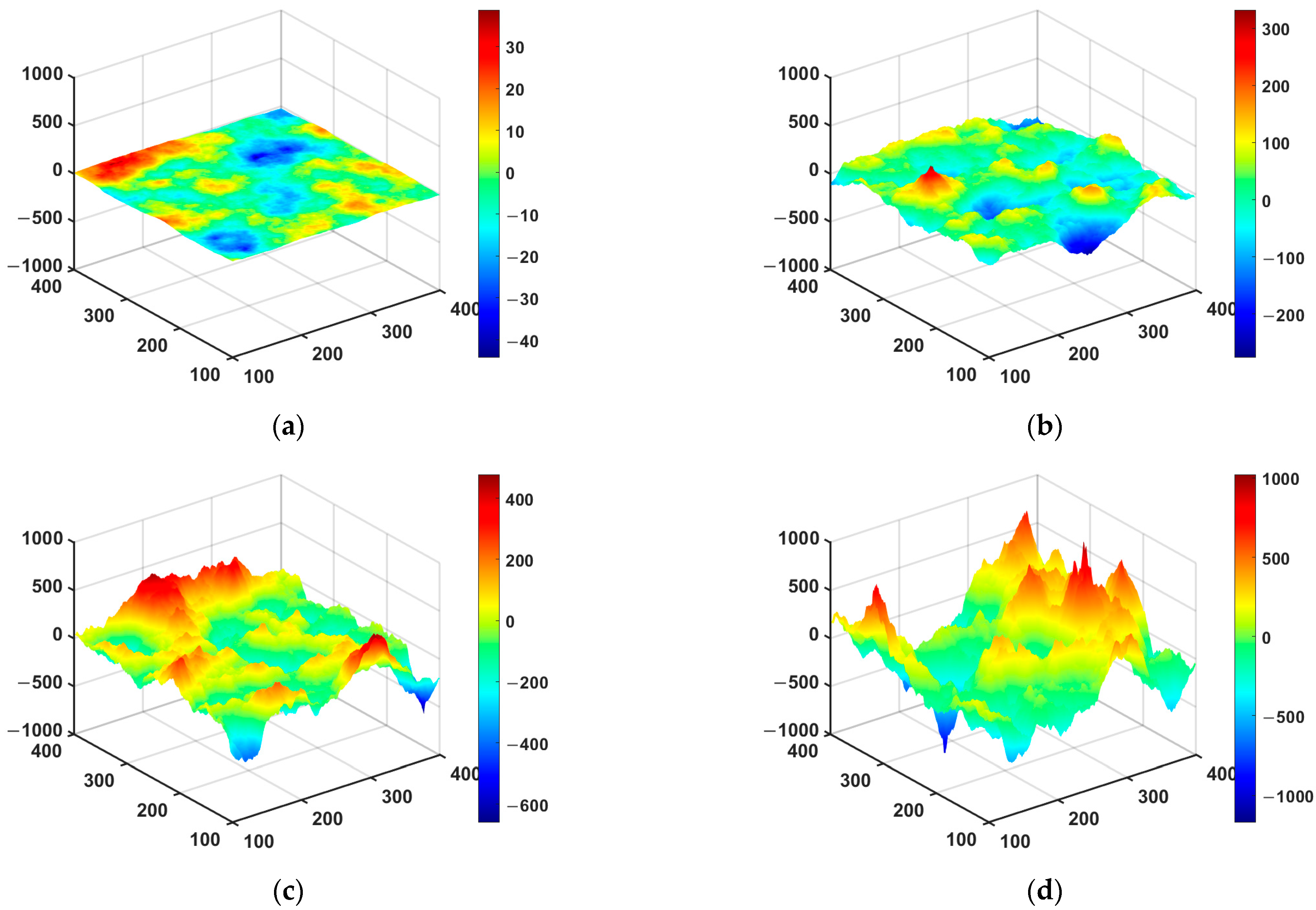
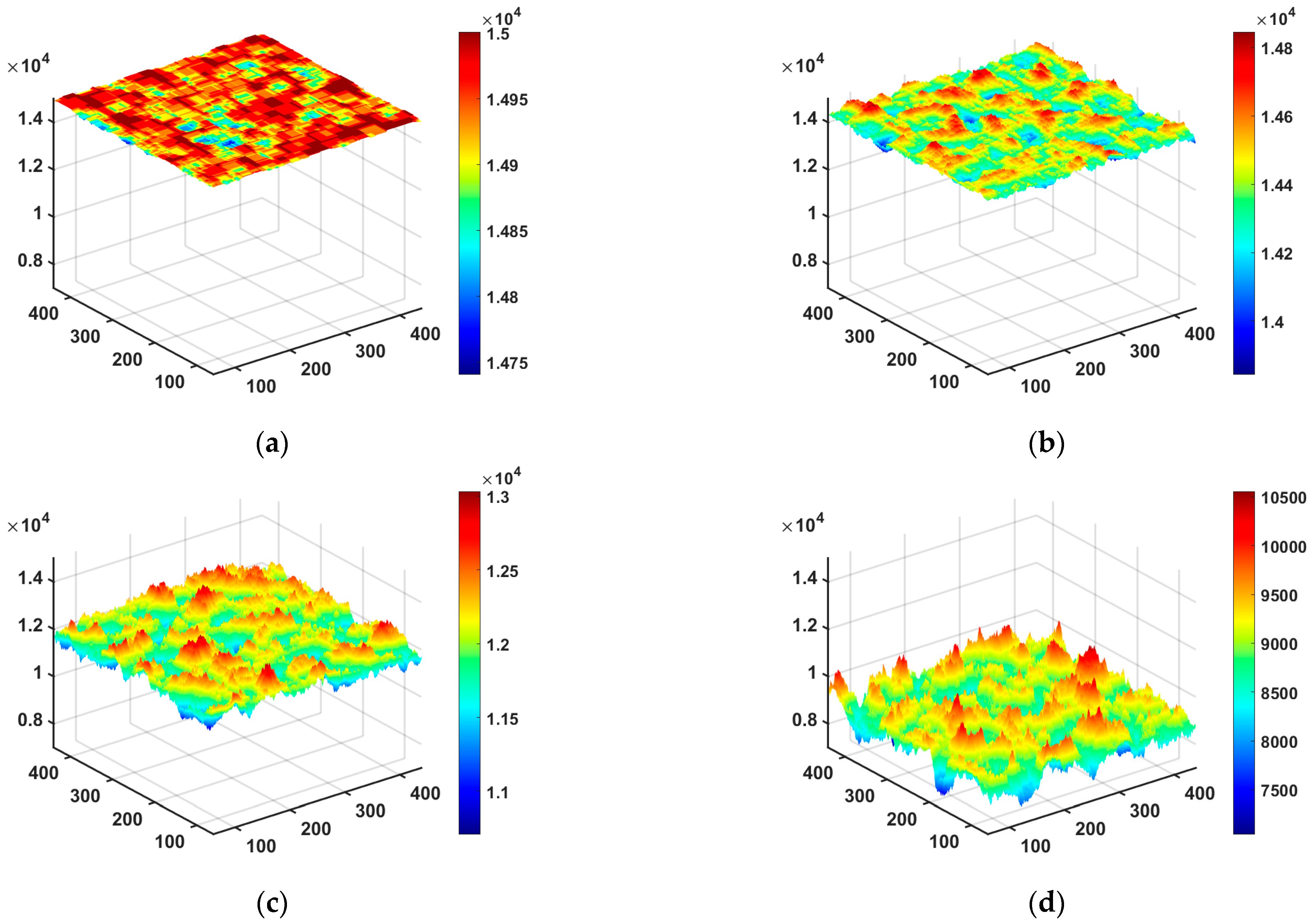
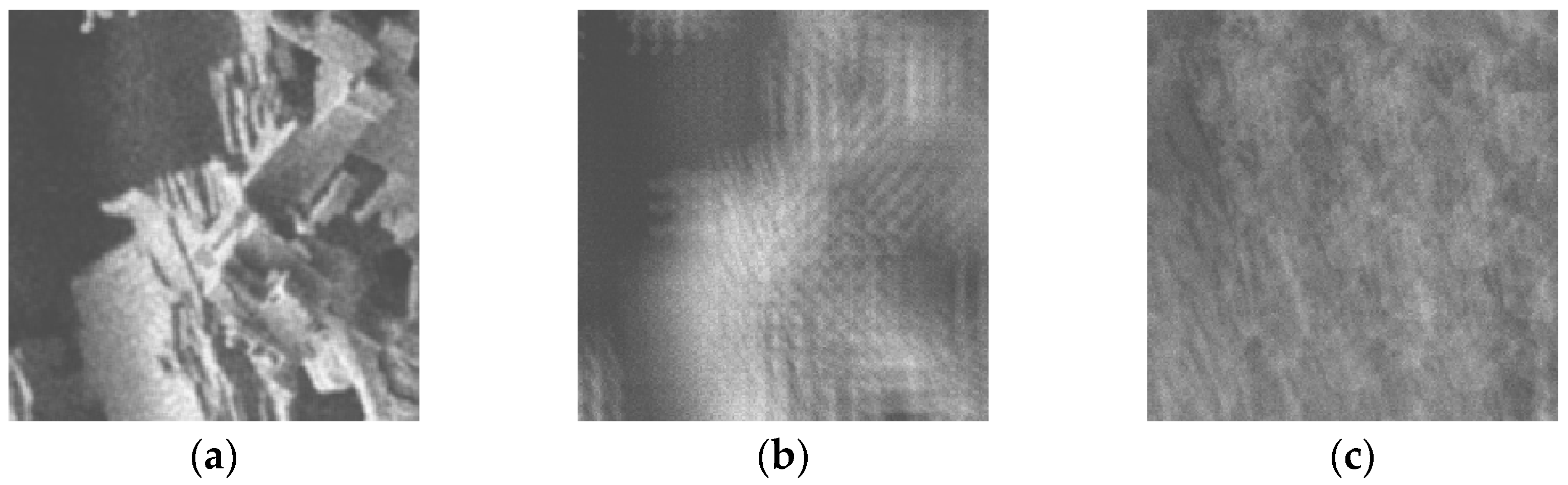
2. Dataset of Rough Surfaces

In this section, we present the data used in this study, beginning with a summary of the algorithms that generated the data, followed by illustrative examples.

The first type of surfaces analyzed in this work is smooth isotropic self-affine (SA) surfaces. These surfaces are created through a stochastic Fourier-transform filtering procedure applied to two-dimensional white-noise height fields [35,36]. In practice, one begins with an uncorrelated Gaussian noise map and prescribes its statistical properties by imposing an isotropic autocorrelation function (ACF):

$$ACF\left(r\right)={RMS}^2{e}^{{-\left(\frac{r}{\xi }\right)}^{2a}},$$

where RMS (the root-mean-square height) sets the overall amplitude of vertical fluctuations, ξ denotes the single correlation length, and α is the roughness exponent. By transforming the noise into the Fourier domain, multiplying each coefficient by the square root of the power spectrum corresponding to this ACF, and then performing an inverse transform, one obtains a height field whose spatial statistics precisely reflect the prescribed RMS, ξ, and α.

RMS governs the absolute range of height variations defining the width of their distribution; therefore, any choice of RMS may be linearly rescaled to a prescribed range without altering the surface’s qualitative morphology. In contrast, ξ and α play the dominant roles in shaping spatial appearance. The correlation length ξ controls the distance over which height values remain correlated: small ξ yields fine-grained, highly intricate patterns, while large ξ produces broader, smoother undulations. The roughness exponent α modulates the balance between high- and low-frequency components, lower α enhances fine-scale, noisy features, and higher α emphasizes coarse-scale, smoother structures.

In this paper, we will focus exclusively on the influence of the root-mean-square amplitude RMS on complexity metrics. By varying RMS across a defined range, we will quantify its effects on a spatial complexity metric that is based on the calculation of multiscale Shannon entropies. Figure 1 shows examples of surfaces generated using this methodology, with varying RMS values and a fixed correlation length and roughness exponent.

The second type of surfaces analyzed in this work is stepwise (SW) surfaces. These are generated by simulating a toy-model for the wet-etching process of a metal surface: starting from a large, solid block cuboid simulating the whole metal material, much smaller cuboids of fixed dimensions are removed one by one at random positions across its top face, each removal event carving out a localized cavity. The cumulative effect of successive removals produces a rugged, terraced landscape analogous to metal surfaces subjected to etching [37].

In this paper, etching time functions as the pivotal parameter: it is quantified by the total number of cuboid removal events and directly governs the evolution of surface morphology. Crucially, as etching time increases, the RMS height of the SW surfaces grows, reflecting the progressive amplification of vertical fluctuations induced by additional material removal though correlation length remains fixed due to the constant size (equal to 30 pixels) of the removed cuboids during etching. Because RMS will also serve as the primary descriptor of SW surface amplitude in our study, we will systematically vary etching time, measure the resulting RMS values, and analyze how changes in RMS alone influence our multiscale Shannon entropy spatial complexity metric.

Figure 2 shows examples of stepwise surfaces generated using the aforementioned methodology, with varying RMS values (that correspond to different etching times). The correlation length is kept fixed during RMS growth and equal to the size of the removed cuboids.

In summary, these two complementary families of synthetic surfaces, smooth self-affine textures generated via Fourier-domain filtering (Figure 1) and terraced, stepwise landscapes produced by simulated cuboid removal (Figure 2), allow us to isolate and systematically probe the role of RMS in driving spatial complexity. By holding, explicitly, the correlation length and roughness exponent constant in the self-affine case, and by varying the etching time (and, thus, RMS) in the stepwise case, we have constructed a controlled dataset in which RMS alone governs the morphological differences. This well-characterized suite of surfaces will form the basis for our multiscale Shannon entropy spatial complexity analysis in the following sections.

3. Methodology

The following subsections detail the computation of an entropy-based spatial complexity metric for surface images. Section 3.1 outlines the multiscale mass field formulation and the derivation of entropy from its distribution, while Section 3.2 examines the impact of histogram binning schemes on entropy estimation, with particular attention to their sensitivity to surface roughness.

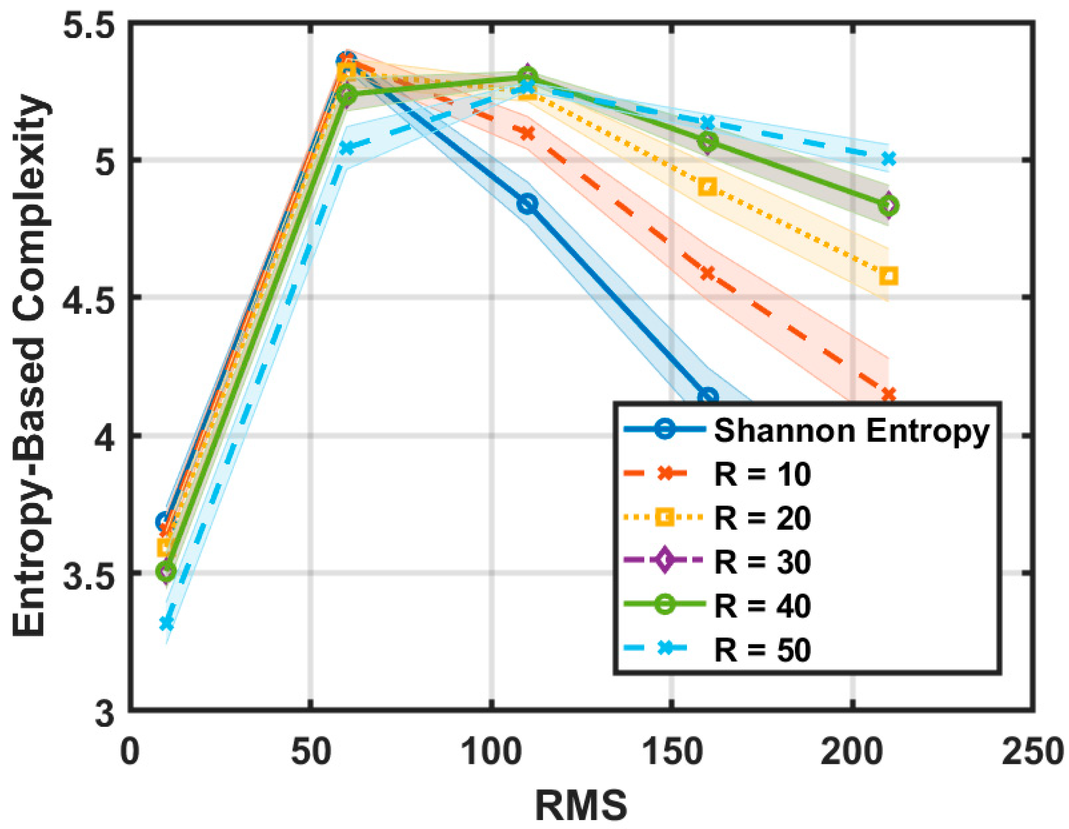
3.1. Calculation of Entropy-Based Complexity

This subsection outlines the methodology used to compute the entropy-based spatial complexity metric and demonstrates its application to surfaces/images for illustrative purposes.

The method [13,38,39] begins with an examination of an initial surface I, focusing individually on each measurement point. The “mass” $m_r(x,y)$ of a measurement point (pixel of surface image) with coordinates (x, y) is computed as the average height of the point itself and its eight neighbors located at the corners and middle of a square with side 2r around it, akin to taking a small group of points and determining their collective average height. The formula that gives the “mass” $m_r\left(x,y\right)$ of a point is the following:

$$m_r(x,y)=\frac{1}{9}\sum _{i\epsilon X} \sum _{j\epsilon Y} I(i,j)$$

where X = {x − r, x, x + r}, Y = {y − r, y, y + r} are the coordinates of the points contributing to the sum of “mass” calculation. This procedure is repeated across different scales r, up to a maximum scale R. To maintain accuracy, pixels near the borders of the surface image are excluded from these calculations. This is a precautionary measure to avoid any distortion that may occur due to these edge pixels having fewer neighbors, which could influence the average brightness calculation. Therefore, to avoid boundary biases, the “mass” field is limited to a region defined by

$$\left(x,y\right)=\left\{\left(x,y\right)∣x\in \left(R+1:L-R\right),y\in \left(R+1:L-R\right)\right\}.$$

An example of the first step of the methodology is displayed in Figure 3 where the “mass” fields of an SEM image are shown calculated for r = 10 (Figure 3b) and r = 50 (Figure 3c).

Next, through the related histograms of the mass distributions, the Shannon entropy $E\left(r\right)=-\sum _i{p}_i\mathit{log}{p}_i$ for each scale r is calculated, where E(r) is quantifying the uniformity in the distribution of mass field values defined within the varying neighborhood sizes. Finally, the entropy-based spatial complexity metric C_en(R) arises by averaging through all the entropies of the distributions over the scales $0<r\le R:$

$$C_{en}(R)=\frac{1}{R}\sum _{r=1}^R E(r)$$

In the calculation of entropy, the histogram of pixel intensities is a critical factor that directly affects the final complexity metric. Both the number of bins and their size determine how the underlying distribution is represented and thus how entropy is computed. This is particularly important when analyzing surfaces of varying roughness since the RMS height influences the spread of values within the histogram. As RMS increases, the distribution of height values or mass values typically widens, and the choice of histogram binning can strongly influence how this change is reflected in the entropy.

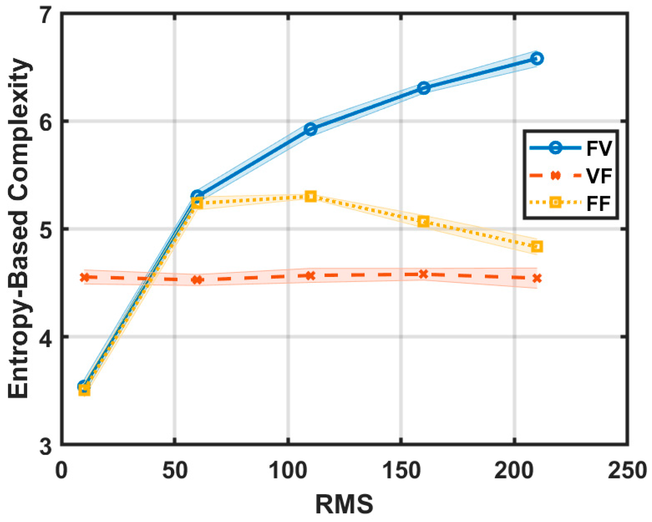
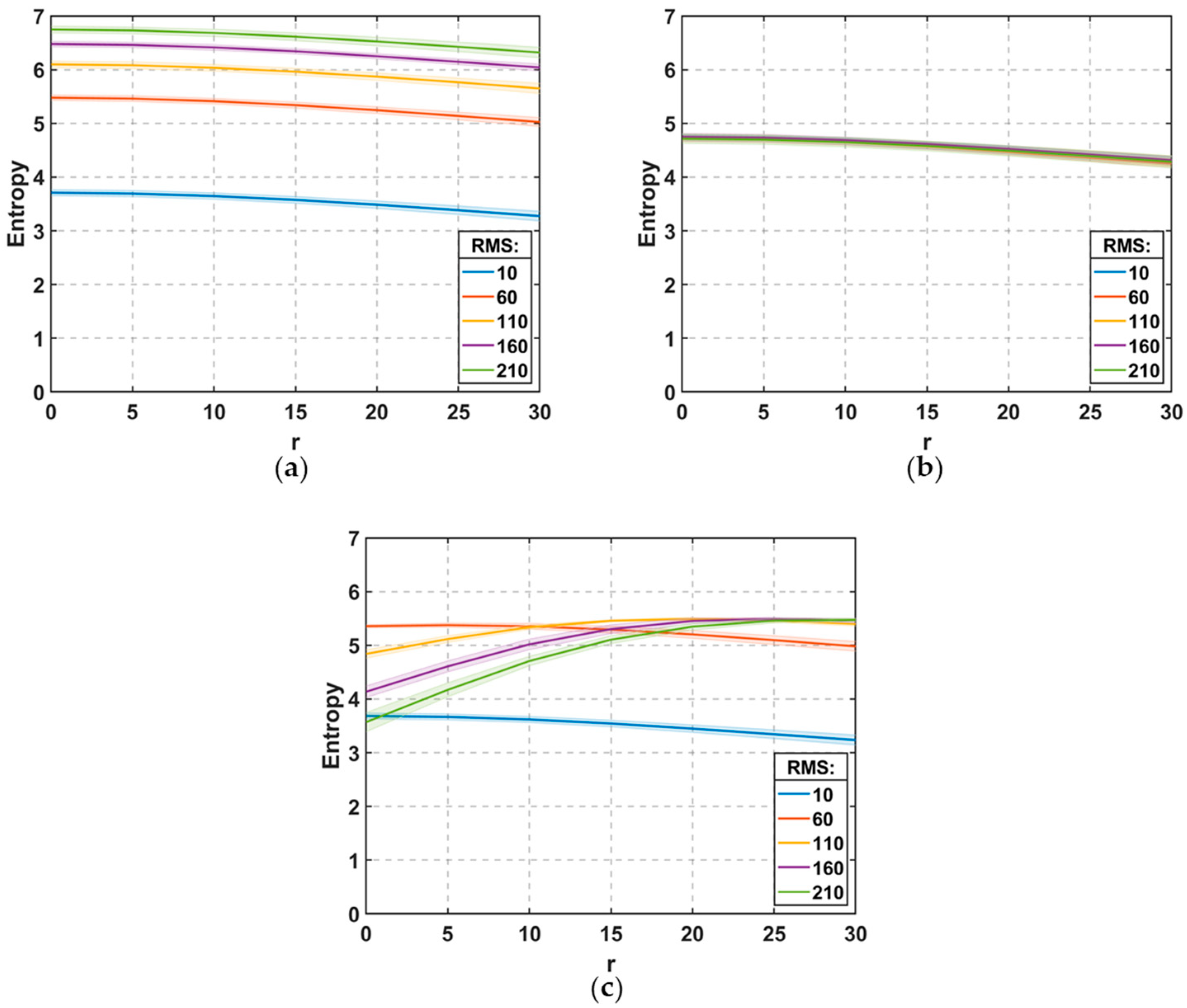
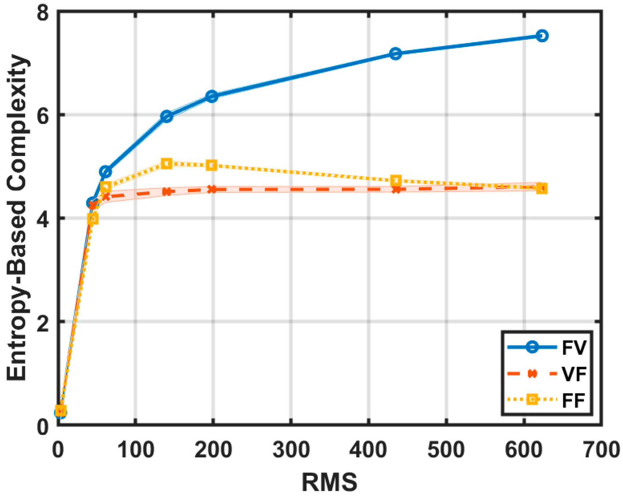
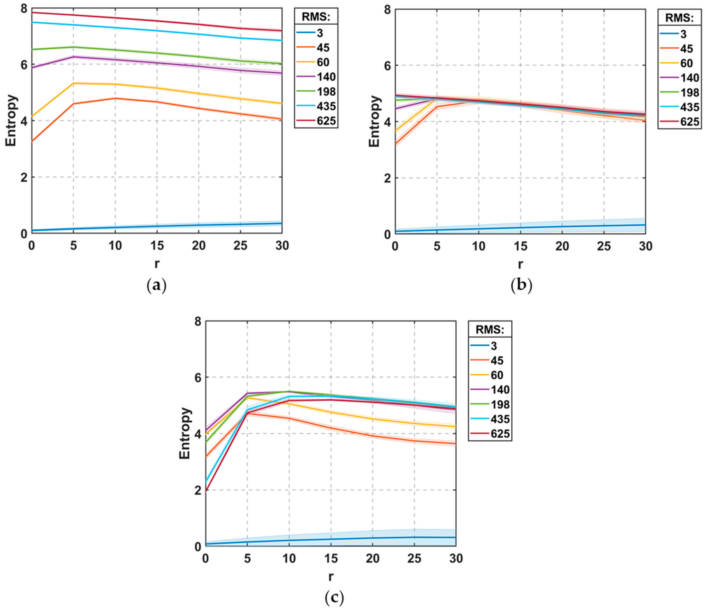
3.2. Binning Schemes

In order to investigate more thoroughly the critical role of binning in surface complexity measurements, we define and apply three schemes to emphasize or exclude RMS effects or resemble the binning used during the imaging of a surface. In the first binning scheme, the bin size is fixed, while the number of bins is allowed to vary depending on the spread of the data. This is referred to as the fixed–variable (FV) case. As RMS increases and the underlying distribution broadens, more bins are introduced to accommodate the extended range of values. This approach captures the growing complexity of the distribution and entropy increases with RMS.

In contrast, the variable–fixed (VF) scheme keeps the number of bins constant while adjusting the bin size to match the data range. As the RMS increases and the data range expands, each bin becomes proportionally wider to ensure full coverage of the distribution. This strategy maintains a consistent histogram structure across different surfaces and RMS values, which tends to stabilize the resulting entropy values. As a result, the entropy in the VF case remains constant even as the RMS changes given that distribution shape remains unaltered.

Finally, the fixed–fixed (FF) scheme keeps both the number of bins and the bin size constant across all surfaces. This approach corresponds to the process in which surface morphology is measured with a microscope and converted into a digital image. In such images, each pixel typically takes a value between 0 and 255 in the case of an 8-bit resolution. Therefore, both the bin size and the number of bins remain fixed during the transformation from the measured surface to the digital representation. The physical meaning of this scheme is directly related to the way a Scanning Electron Microscope captures and digitizes surface information on micro and nanoscale.

In this case, as RMS increases and the distribution exceeds the predefined histogram range, values that fall outside the bounds are remapped to the edges of the distribution. Entropy initially increases with RMS due to the natural broadening of the distribution, but beyond a critical value RMS*, where the total width of the distribution exceeds the capacity of the histogram, this remapping begins to distort the histogram. As a result, entropy increases until the critical value of RMS* and then decreases as the distribution becomes artificially skewed at the ends due to the addition of pixels at the tails.

To sum up, surface complexity has an amplitude part that tracks height variations and a spatial part that tracks their spatial arrangement. The FV binning keeps the bin width constant and lets the number of bins grow so that it captures both parts. The VF binning keeps the bin count constant while allowing the bin width to expand. This approach removes most of the amplitude influence and emphasizes the complexity of the spatial organization of surface heights. The FF binning locks both the bin count and width to the detector grayscale, thus showing how complexity appears in the recorded image of a rough surface, including any clipping of extreme heights.

4. Results and Discussion

In the following subsections, we present and analyze the results of our entropy-based spatial complexity metric as applied to the two categories of surfaces. Section 4.1 focuses on self-affine surfaces where we systematically examine how increasing RMS amplitude affects complexity under different histogram discretization (i.e., binning) schemes. Section 4.2 investigates stepwise surfaces produced through a simulated etching process, with an emphasis on how complexity varies as a function of RMS. These sections collectively demonstrate how the proposed complexity measure responds to controlled changes in surface topography.

4.1. Self-Affine Surfaces

To evaluate how entropy-based spatial complexity responds to controlled variations in surface amplitude, we begin by analyzing the family of self-affine surfaces described in Section 2. These surfaces are generated with a constant correlation length and roughness exponent, allowing us to isolate the effect of RMS height on the complexity measure. Using the methodology outlined in Section 3, we compute multiscale Shannon entropy across various spatial scales r, then average these values to obtain a single complexity score for each surface.

A key factor influencing the entropy calculation is the choice of binning strategy used to compute the mass distribution. We examine the three aforementioned schemes: fixed–variable (FV), variable–fixed (VF), and fixed–fixed (FF). Each approach affects the resulting complexity measure differently, depending on how the histogram bins interact with the evolving distribution of pixel intensities as RMS increases.

The results from the three binning schemes are illustrated in Figure 4, which presents the entropy-based spatial complexity as a function of RMS height. Complementary plots of entropy versus spatial scale r for each binning strategy are shown in Figure 5, providing a detailed view of scale-dependent behavior across the different discretization approaches.

More specifically, in the FV case, where the bin size is held constant and the number of bins grows with the range of data, we observe a clear and consistent increase in entropy-based complexity with rising RMS. As the distribution of brightness values becomes broader, additional bins are introduced to capture finer variations. This increase in the number of involved bins leads to higher entropy at each scale and, therefore, a higher average complexity value (see Figure 4). Notably, as Figure 5a shows, this trend is preserved across all scales r, underscoring the FV scheme’s sensitivity to amplitude-driven changes in surface morphology.

In contrast, the VF scheme maintains a fixed number of bins while allowing their size to expand in proportion to the range of pixel values. This adaptive scaling stabilizes the structure of the histogram, yielding nearly constant entropy values across different RMS levels. Because the entire distribution is consistently captured, albeit with coarser bins as RMS grows, the resulting complexity metric is largely unaffected by changes in surface amplitude (see Figure 4 and Figure 5b).

The FF scheme, in which both the number of bins and their size are fixed, exhibits a more nuanced behavior. At low RMS values, entropy increases as expected due to the broadening of the mass distribution. However, beyond a certain threshold, where the spread of values exceeds the range accommodated by the histogram, this trend reverses. Values falling outside the histogram bounds are clipped and remapped to the distribution edges, creating artificial peaks and reducing entropy. The result is a non-monotonic complexity curve that peaks at an intermediate RMS (RMS* ≈ 60–100) and then declines (Figure 4). This behavior reflects not a physical reduction in surface complexity but a distortion introduced by the binning limitations. The E(r) curves presented in Figure 5c demonstrate that the observed decline in complexity for RMS > RMS* arises from a reduction in entropy at small r values, corresponding to the formation of flat regions at the upper and lower boundaries of the image-like surface following FF binning scheme.

These results highlight the crucial role that discretization choices play in interpreting entropy-based complexity. The FV scheme accurately tracks complexity growth with increasing RMS, making it suitable when surface amplitude is a variable of interest. The VF scheme offers stability and comparability across surfaces of differing amplitudes, emphasizing the impact of spatial aspects of roughness, while the FF scheme, although simpler to implement, may introduce artifacts once the surface variability exceeds its predefined bounds.

The observed trends are consistent with analytical expectations for Gaussian distributions [40]. Specifically, entropy remains constant when bin counts adaptively match the spread of a widening distribution (as in the VF case) but decreases when the distribution’s tail is truncated due to fixed bin limits (as in the FF case). Collectively, these findings establish a foundational understanding of how multiscale entropy responds to changes in amplitude and guide the selection of appropriate binning schemes depending on the specific aspect of surface complexity being quantified.

In the FF case, the non-monotonic behavior of the E(r) curves with respect to RMS shown in Figure 5c implies that the choice of scale range R plays a critical role in determining the final complexity value. As illustrated in Figure 6, the entropy-based spatial complexity curve as a function of RMS shifts depending on the selected R. Specifically, the peak of the curve tends to move toward higher RMS values and becomes more diffuse as R increases, effectively smoothing out the pronounced maximum observed at smaller scales.

4.2. Stepwise Surfaces

We next apply the entropy-based spatial complexity analysis to the family of stepwise surfaces introduced in Section 2. Unlike the self-affine surfaces, which originate from Gaussian-distributed height fields, stepwise surfaces evolve from an initially flat substrate into increasingly rugged textures through a stochastic etching process. As etching progresses and small cuboids are randomly removed from the surface, the RMS height increases, introducing greater amplitude-based morphological complexity since correlation length remains fixed. In this section, we focus specifically on how the multiscale complexity metric responds to changes in RMS amplitude.

Similar to the self-affine case, three histogram discretization schemes are considered: fixed–variable (FV), variable–fixed (VF), and fixed–fixed (FF). Each scheme shapes how the mass distributions are interpreted and thus influences the observed entropy values. The results are illustrated in Figure 7, which presents entropy-based spatial complexity as a function of RMS height for the three binning schemes.

In the FV scheme, complexity increases steadily with RMS. This reflects the growing diversity in the mass distribution as the surface transitions from a nearly flat morphology to one with numerous etched pits. Initially, when the surface is largely smooth, the distribution is narrow and entropy is low at all scales. As etching progresses, more pits emerge and the amplitude distribution widens, necessitating more histogram bins under the FV scheme. The added bins allow the metric to detect increasingly fine-grained variations, leading to higher entropy values across scales. While the surfaces do not begin with Gaussian characteristics, the logic of entropy growth with increasing distribution width still applies.

The VF scheme again yields entropy values that are largely stable across RMS variations. By maintaining a fixed number of histogram bins and adjusting their width to cover the full dynamic range, the structure of the histogram remains consistent despite changes in the underlying mass distribution. Even as the surface evolves and the distribution of values broadens, the entropy calculation adapts through bin width adjustment, producing minimal variation in the final complexity metric. It is worth noting that during the initial stages of the simulation, when the surface is nearly flat and RMS values are low, the complexity exhibits an increasing trend. This is due to the transition from a Poisson-like distribution at the initial stages of surface evolution to a more Gaussian-like distribution observed at greater etching times and higher RMS values. This transition underscores the capability of the VF scheme to capture changes in the histogram morphology of surface amplitudes.

The FF scheme, as in the self-affine case, produces a non-monotonic complexity trend. Initially, entropy increases with RMS as the histogram begins to capture the growing range of pixel values associated with pit formation. However, once the distribution exceeds the fixed bin range, values falling outside the bounds are clipped to the edges, resulting in a loss of representational fidelity. This artificial compression leads to reduced entropy values despite increasing surface disorder. As complexity aims to quantify information content, this drop reflects an underestimation caused by the histogram’s inability to encode the full distribution once it exceeds its limits.

These trends are further clarified by the entropy versus scale E(r) plots shown in Figure 8. In the FV binning scheme (Figure 8a), as RMS increases, entropy values grow at all scales r due to the emergence and multiplication of smaller flat regions that locally break uniformity. In contrast to self-affine surfaces, the entropy curves do not exhibit a monotonically decreasing trend across all RMS values (cf. Figure 5a). At lower RMS values, the prevalence of large, flat terraces preserves a high degree of local homogeneity, thereby maintaining relatively low entropy levels. This results in the emergence of a broad maximum in the E(r) curves at intermediate scales, corresponding to the average width of these flat terraces. As etching proceeds and the terraces become increasingly fragmented, local variability intensifies, causing the maximum to shift toward smaller scales until it ultimately vanishes at sufficiently high RMS values.

A similar trend is observed in the VF scheme; however, the E(r) curves appear generally squeezed due to the suppression of RMS-related effects, particularly at high RMS values (Figure 8b). Notably, at low RMS values, one can still observe the gradual disappearance of the broad peak, reflecting the transition from surfaces characterized by flat terraces and a Poisson-like amplitude distribution to those with smaller pit sizes, increased local variability, and a distribution approaching Gaussian behavior.

A more intricate behavior of the E(r) curves as a function of RMS emerges within the FF scheme due to the additional effect imposed by the fixed histogram range limitation. At small scales, entropy is defined by the extent of flat regions on the etched surfaces. As in the other schemes, increasing RMS leads to the fragmentation of flat terraces into smaller pits via the random etching process, thereby elevating entropy. However, at high RMS values, the fixed histogram range reintroduces prominent flat regions, resulting in a reduction in entropy and the non-monotonic behavior observed in the E(r) curves at small scales (cf. Figure 8c). This effect is attenuated at larger scales, where the monotonic increase of entropy with RMS is progressively restored. These interactions account for the complex crossing patterns of the E(r) curves in the FF scheme and underpin the emergence of the broad maximum in the complexity versus RMS relationship depicted in Figure 7.

Overall, these results emphasize that the entropy-based complexity metric captures both the structural richness introduced by the etching process and the limitations imposed by histogram discretization. The FV scheme effectively tracks the increase in complexity of the whole surface including amplitude effects. The VF scheme provides consistent results across varying RMS values quantifying mainly spatial aspects of surface morphology and changes in amplitude distribution shape. The FF scheme, mimicking the imaging process of a surface, underrepresents complexity at high RMS due to truncation of information. These findings highlight the versatility of the proposed metric and its capacity to reflect subtle morphological transitions even in non-Gaussian, process-driven surfaces.

In the FF case, the non-monotonic behavior of the E(r) curves with respect to RMS implies that the choice of scale range R plays a critical role in determining the final complexity value, as also observed previously in the self-affine surfaces. As illustrated in Figure 9, the entropy-based spatial complexity curve as a function of RMS shifts depending on the selected R. Specifically, the peak of the curve becomes more diffuse as R increases, effectively smoothing out the maximum observed at smaller scales.

5. Conclusions

In this study, we elaborated a multiscale entropy-based spatial complexity metric for quantifying the morphological complexity of rough surfaces. The focus has been on the impact of the binning scheme to reveal and quantify different aspects of surface complexity. By analyzing both self-affine and stepwise surfaces, we established a clear relationship between RMS amplitude and entropy-based complexity under different histogram binning schemes. In particular, the fixed–variable (FV) scheme proved highly sensitive to amplitude-driven changes enabling the quantification of surface complexity including amplitude effects, while the variable–fixed (VF) scheme offered consistent measurements across varying RMS values and seems to be the proper scheme for capturing spatial aspects of surface complexity alone. The fixed–fixed (FF) scheme highlighted important limitations in representational fidelity when the dynamic range of surface variations exceeded the binning capacity. Overall, the developed framework offers a scale-sensitive method for characterizing structural complexity in topographical datasets.

This study also has some limitations that warrant further investigation. Up to now, the method has only been applied to synthesized rough surfaces, so it will be important to apply it to real surfaces measured with an Atomic Force Microscope, for example, to validate its practical utility. Additionally, in future work, we aim to explore the use of more and different entropy measures to enhance the sensitivity and interpretability of the results. Finally, it is worth noting that the distribution function of surface heights depends not only on its second moment (RMS value) but also on higher-order moments such as skewness and kurtosis, which could be systematically incorporated into the analysis framework.

References

1. Zhao, Y.; Wang, G.C.; Lu, T.M. Characterization of Amorphous and Crystalline Rough Surface—Principles and Applications; Elsevier: Amsterdam, The Netherlands, 2000; Volume 37. [Google Scholar]
2. Almqvist, A. On the Effects of Surface Roughness in Lubrication; LAP Lambert Academic Publishing: Saarbrücken, Germany, 2009. [Google Scholar]
3. Vander Voort, G.F. Metallography, Principles and Practice; ASM International: Materials Park, OH, USA, 1999. [Google Scholar]
4. Zhou, W.; Apkarian, R.; Wang, Z.L.; Joy, D. Fundamentals of scanning electron microscopy (SEM). In Scanning Microscopy for Nanotechnology: Techniques and Applications; Springer: New York, NY, USA, 2007; pp. 1–40. [Google Scholar]
5. Vernon-Parry, K.D. Scanning electron microscopy: An introduction. III-Vs Rev. 2000, 13, 40–44. [Google Scholar] [CrossRef]
6. Barabási, A.L.; Stanley, H.E. Fractal Concepts in Surface Growth; Cambridge University Press: Cambridge, UK, 1995. [Google Scholar]
7. Barnsley, M.F. Fractals Everywhere; Academic Press: Cambridge, MA, USA, 2014. [Google Scholar]
8. Sarkar, N.; Chaudhuri, B.B. An efficient differential box-counting approach to compute fractal dimension of image. IEEE Trans. Syst. Man Cybern. 1994, 24, 115–120. [Google Scholar] [CrossRef]
9. Florindo, J.B.; Sikora, M.S.; Pereira, E.C.; Bruno, O.M. Characterization of nanostructured material images using fractal descriptors. Phys. A Stat. Mech. Its Appl. 2013, 392, 1694–1701. [Google Scholar] [CrossRef]
10. Liu, Y.U.; Chen, L.; Wang, H.; Jiang, L.; Zhang, Y.; Zhao, J.; Wang, D.; Zhao, Y.; Song, Y. An improved differential box-counting method to estimate fractal dimensions of gray-level images. J. Vis. Commun. Image Represent. 2014, 25, 1102–1111. [Google Scholar] [CrossRef]
11. Kondi, A.; Papia, E.M.; Stai, E.; Constantoudis, V. Computational methods in nanometrology: The challenges of resolution and stochasticity. Front. Nanotechnol. 2025, 7, 1559523. [Google Scholar] [CrossRef]
12. Kondi, A.; Constantoudis, V.; Sarkiris, P.; Ellinas, K.; Gogolides, E. Using chaotic dynamics to characterize the complexity of rough surfaces. Phys. Rev. E 2023, 107, 014206. [Google Scholar] [CrossRef] [PubMed]
13. Arapis, A.; Constantoudis, V.; Kontziampasis, D.; Milionis, A.; Lam, C.W.E.; Tripathy, A.; Poulikakos, D.; Gogolides, E. Measuring the complexity of micro and nanostructured surfaces. Mater. Today Proc. 2022, 54, 63–72. [Google Scholar] [CrossRef]
14. Bagrov, A.A.; Iakovlev, I.A.; Iliasov, A.A.; Katsnelson, M.I.; Mazurenko, V.V. Multiscale structural complexity of natural patterns. Proc. Natl. Acad. Sci. USA 2020, 117, 30241–30251. [Google Scholar] [CrossRef] [PubMed]
15. Wang, P.; Gu, C.; Yang, H.; Wang, H.; Moore, J.M. Characterizing systems by multi-scale structural complexity. Phys. A Stat. Mech. Its Appl. 2023, 609, 128358. [Google Scholar] [CrossRef]
16. Srenevas, S.; Poutous, M.K. Shannon’s entropy and structural complexity of random antireflective nanostructures on fused silica surfaces. In Nanoengineering: Fabrication, Properties, Optics, Thin Films, and Devices XX; SPIE: San Diego, CA, USA, 2023; Volume 12653, pp. 70–79. [Google Scholar]
17. Kim, D.; Choi, J.; Nam, J. Entropy-assisted image segmentation for nano-and micro-sized networks. J. Microsc. 2016, 262, 274–294. [Google Scholar] [CrossRef] [PubMed]
18. Srenevas, S.; Poutous, M.K. Complexity Imbalance of Nanostructured Antireflective Surfaces. In Proceedings of the 2024 Conference on Lasers and Electro-Optics (CLEO), Charlotte, NC, USA, 5–10 May 2024; IEEE: Piscataway, NJ, USA, 2024; pp. 1–2. [Google Scholar]
19. Lakhal, S.; Darmon, A.; Bouchaud, J.P.; Benzaquen, M. Beauty and structural complexity. Phys. Rev. Res. 2020, 2, 022058. [Google Scholar] [CrossRef]
20. Andraud, C.; Beghdadi, A.; Haslund, E.; Hilfer, R.; Lafait, J.; Virgin, B. Local entropy characterization of correlated random microstructures. Phys. A Stat. Mech. Its Appl. 1997, 235, 307–318. [Google Scholar] [CrossRef]
21. Van Siclen, C.D. Information entropy of complex structures. Phys. Rev. E 1997, 56, 5211. [Google Scholar] [CrossRef]
22. Ruiz, R.L.; Mancini, H.; Calbet, X. A statistical measure of complexity. In Concepts and Recent Advances in Generalized Information Measures and Statistics; Bentham Science Publishers: Sharjah, United Arab Emirates, 2013; pp. 147–168. [Google Scholar]
23. Alamino, R.C. Measuring complexity through average symmetry. J. Phys. A Math. Theor. 2015, 48, 275101. [Google Scholar] [CrossRef]
24. Zanette, D.H. Quantifying the complexity of black-and-white images. PLoS ONE 2018, 13, e0207879. [Google Scholar] [CrossRef] [PubMed]
25. Nicolis, G.; Nicolis, C. Foundations of Complex Systems: Emergence, Information and Predicition; World Scientific: Singapore, 2012. [Google Scholar]
26. Ladyman, J.; Lambert, J.; Wiesner, K. What is a complex system? Eur. J. Philos. Sci. 2013, 3, 33–67. [Google Scholar] [CrossRef]
27. Gell-Mann, M. What is complexity? In Complexity and Industrial Clusters: Dynamics and Models in Theory and Practice; Physica-Verlag HD: Heidelberg, Germany, 2002; pp. 13–24. [Google Scholar]
28. Mitchell, M. Complexity: A Guided Tour; Oxford University Press: Oxford, UK, 2009. [Google Scholar]
29. Shannon, C.E. A mathematical theory of communication. Bell Syst. Tech. J. 1948, 27, 379–423. [Google Scholar] [CrossRef]
30. Cover, T.M. Elements of Information Theory; John Wiley & Sons: Hoboken, NJ, USA, 1999. [Google Scholar]
31. Rényi, A. On measures of entropy and information. In Proceedings of the Fourth Berkeley Symposium on Mathematical Statistics and Probability, Volume 1: Contributions to the Theory of Statistics, Berkeley, CA, USA, 20–30 July 1960; University of California Press: Berkeley, CA, USA, 1961; Volume 4, pp. 547–562. [Google Scholar]
32. Gray, R.M. Entropy and Information Theory; Springer Science & Business Media: Berlin/Heidelberg, Germany, 2011. [Google Scholar]
33. Freedman, D.; Diaconis, P. On the histogram as a density estimator: L 2 theory. Z. Wahrscheinlichkeitstheorie Verwandte Geb. 1981, 57, 453–476. [Google Scholar] [CrossRef]
34. Gonzalez, R.C.; Woods, R.E. Digital Image Processing, 4th ed.; Pearson: London, UK, 2018. [Google Scholar]
35. Yang, G.; Li, B.; Wang, Y.; Hong, J. Numerical simulation of 3D rough surfaces and analysis of interfacial contact characteristics. CMES 2014, 103, 251–279. [Google Scholar]
36. Wang, Y.; Azam, A.; Wilson, M.C.; Neville, A.; Morina, A. Generating fractal rough surfaces with the spectral representation method. Proc. Inst. Mech. Eng. Part J J. Eng. Tribol. 2021, 235, 2640–2653. [Google Scholar] [CrossRef]
37. Sarkiris, P.; Constantoudis, V.; Ellinas, K.; Lam, C.W.E.; Milionis, A.; Anagnostopoulos, J.; Poulikakos, D.; Gogolides, E. Topography optimization for sustainable dropwise condensation: The critical role of correlation length. Adv. Funct. Mater. 2024, 34, 2306756. [Google Scholar] [CrossRef]
38. Papia, E.M.; Kondi, A.; Constantoudis, V. Entropy and complexity analysis of AI-generated and human-made paintings. Chaos Solitons Fractals 2023, 170, 113385. [Google Scholar] [CrossRef]
39. Veinidis, C.N.; Akriotou, M.; Kondi, A.; Papia, E.M.; Constantoudis, V.; Syvridis, D. Complexity analysis of challenges and speckle patterns in an Optical Physical Unclonable Function. Chaos Solitons Fractals 2025, 191, 115938. [Google Scholar] [CrossRef]
40. Available online: https://gregorygundersen.com/blog/2020/09/01/gaussian-entropy/ (accessed on 21 July 2025).
Figure 1. Self-affine rough surfaces with RMS roughness values of (a) 10, (b) 75, (c) 150, and (d) 225, with a correlation length of 40 and a roughness exponent of 0.8 in all cases.
Mathematics 13 02325 g001
Figure 2. Stepwise surfaces at different etching times, with corresponding RMS roughness values of (a) 45, (b) 145, (c) 335, and (d) 420.
Mathematics 13 02325 g002
Figure 3. An example of the effect that the entropy-based spatial complexity measure has in a SEM image (1 μm × 1 μm) of an etched metal surface for different scales (r): (a) original SEM image, (b) the “mass” field of the original SEM image calculated for a scale r = 10, and (c) the “mass” field for a scale r = 50.
Mathematics 13 02325 g003
Figure 4. Entropy-based spatial complexity as a function of RMS height for self-affine surfaces. The three curves correspond to the fixed–variable (FV) binning where complexity rises steadily with RMS, the variable–fixed (VF) binning where complexity stays nearly constant, and the fixed–fixed (FF) binning, which displays a broad peak around RMS 60 to 100 followed by a decline.
Mathematics 13 02325 g004
Figure 5. Entropy as a function of spatial scale r for self-affine surfaces, shown separately for each binning scheme: (a) fixed–variable (FV), (b) variable–fixed (VF), and (c) fixed–fixed (FF). The FV curves grow at every scale with increasing RMS, the VF curves nearly overlap, and the FF curves show a non-monotonic intricate behavior.
Mathematics 13 02325 g005
Figure 6. Entropy-based spatial complexity vs. RMS height for the fixed–fixed (FF) binning scheme, shown for different maximum scale values R. Increasing R shifts the peak complexity toward higher RMS values and smooths the overall curve, highlighting the sensitivity of the final complexity measure to the chosen scale range.
Mathematics 13 02325 g006
Figure 7. Entropy-based spatial complexity as a function of RMS height for stepwise surfaces. The FV curve rises monotonically, while the VF curve remains almost flat except for a gentle increase at low RMS linked to the Poisson to Gaussian transition. In contrast, the FF curve climbs then falls once the amplitude distribution extends beyond the fixed histogram limits.
Mathematics 13 02325 g007
Figure 8. Entropy as a function of spatial scale r for stepwise surfaces, shown separately for each binning scheme: (a) fixed–variable (FV), (b) variable–fixed (VF), and (c) fixed–fixed (FF). The FV scheme (a) shows a peak that moves to smaller r as etching advances, the VF scheme (b) reproduces this trend with reduced amplitude, and the FF scheme (c) displays complex curve crossings caused by clipping of extreme heights at high RMS.
Mathematics 13 02325 g008
Figure 9. Entropy-based spatial complexity vs. RMS height for the fixed–fixed (FF) binning scheme, shown for different maximum scale values R. As R increases, the complexity peak becomes broader and less pronounced, reflecting a smoothing effect introduced by larger-scale ranges.
Mathematics 13 02325 g009
Disclaimer/Publisher’s Note: The statements, opinions and data contained in all publications are solely those of the individual author(s) and contributor(s) and not of MDPI and/or the editor(s). MDPI and/or the editor(s) disclaim responsibility for any injury to people or property resulting from any ideas, methods, instructions or products referred to in the content.