Local Streamline Pattern and Topological Index of an Isotropic Point in a 2D Velocity Field

Abstract

In fluid mechanics, most studies on flow structure analysis are simply based on the velocity gradient, which only involves the linear part of the velocity field and does not focus on the isotropic point. In this paper, we are concerned with a general polynomial velocity field with a nonzero linear part and study its streamline pattern around an isotropic point, i.e., the local streamline pattern (LSP). A complete classification of LSPs in two-dimensional (2D) velocity fields is established. By proposing a novel formulation of qualitative equivalence, namely, the invariance under spatiotemporal transformations, we first introduce the quasi-real Schur form to classify the linear part of velocity fields. Then, for a nonlinear velocity field, the topological type of its LSP is either completely determined by the linear part when the determinant of the velocity gradient at the isotropic point is nonzero or controlled by both linear and nonlinear parts when the determinant of the velocity gradient vanishes at the isotropic point. Four new topological types of LSPs through detailed sector analysis are identified. Finally, we propose a direct method for calculating the index of the isotropic point, which also serves as a fundamental topological property of LSPs. These results do challenge the conventional linear analysis paradigm that simply neglects the contribution of the nonlinear part of the velocity field to the streamline pattern.

1. Introduction

Our understanding of the flow of real fluids, such as air, water, etc., has greatly influenced our viewpoint about the world; meanwhile, the accurate prediction of complex flows, such as in the presence of turbulence, remains a challenge for human intelligence to this day [1,2]. Macroscopic velocity, defined as the statistical average of the velocities of a large number of fluid particulates centered at a point, can be used to describe the movement of identifiable pieces of matter. Batchelor [3] considered that the initial linear dimensions of a fluid element must be so small as to guarantee smallness at all relevant subsequent instants, in spite of the distortions and extensions of the element. However, if we define pieces of fluid with any finite scale at a certain time in a flow, e.g., two pieces along the direction perpendicular to the mainstream in a Couette flow between two plates, then the shear process will keep them as a whole, respectively, but the distance between them cannot be limited forever. On the other hand, considering the fact that fluid particulates cannot maintain their aggregation during the flow [4], it is reasonable to regard the fluid flow as the mutual sliding of fluid layers at the molecular level; so, the viscous friction occurs as the response of the fluid slip strength, such that new fields, in addition to the velocity field, could be introduced to describe the slip contact relationship of fluid layers forming and remaining active during flow [5]. Then, flow field analysis would not be confined to velocity analysis, and the streamline pattern from the velocity direction possesses more implications for the slip structures in the fluid.

Most flow analyses in fluid dynamics are based on the velocity gradient, neglecting the locality of flow structures. Recent advances using real Schur decomposition to extract vortex features [6,7] further entrench this linear paradigm. The streamline pattern is qualitatively defined [8] and in fact equivalent to the phase portrait in dynamics system. Most concepts developed in dynamical systems can be naturally used in the study of streamline patterns in fluid mechanics. Like the phase portrait near a critical point, the local streamline pattern (LSP), namely, the streamline pattern near an isotropic point, must play a crucial role in flow structure analyses. Recently, some novel LSPs, e.g., those characterized by a cusp and a saddle–node, were numerically demonstrated by Brøns [9] and Li et al. [10], respectively, and are unavailable in the analyses of the velocity gradient. These LSPs expose a critical question: can the influence of nonlinear terms really be ignored in streamline pattern analysis? This fact motivated the study presented in this paper.

Three-dimensional polynomial autonomous dynamical systems are quite complicated, exhibiting all the types of behavior of 2D systems, plus much more complicated behaviors [11]. See the following 2D polynomial system:

$${\dot{x}}_1=v_1\left(x_1,x_2\right), {\dot{x}}_2=v_2\left(x_1,x_2\right),$$

(1)

where $v_1$ and $v_2$ are polynomials of $x_1$ and $x_2$ and consist of a vector field. Some important questions remain to be answered beyond the field of linear differential equations [12,13].

This paper will focus on the LSPs of 2D velocity fields with a nonzero linear part, including their classification and index calculation. In Section 2, we first introduce some concepts that are necessary to expand our analysis, such as isotropic point, index, separatrix, sectors, various transformations, etc., where the invariance under a series of transformations of spatiotemporal coordinates is used to define their qualitative classification; in addition, the positive definite transformation of velocity is adopted to carry out the topological equivalence with the same index. In Section 3, the types of linear velocity fields are revisited on the basis of the transformation definition, and in Section 4, we study nonlinear velocity fields with a nonzero linear part through the detailed analyses of sectors, even using the polar blow-up technique. In Section 5, we develop a novel method to compute the index of the velocity field at the isotropic point. Finally, some conclusions are presented.

2. Concept Preparation

An isotropic point is defined as an isolated point in fluid through which no streamline or more than one streamline passes. In order to study the streamline features near an isotropic point in 2D flows, we present the polynomial expression of velocity fields and their qualitative classification, with special emphasis on those with the nonlinear terms.

Assuming that the velocity $\left(v_1,v_2\right)$ in (1) is analytic in the plane $\left(x_1,x_2\right)$ and takes the origin as one of its isotropic points, we have

$$v_1=P_m\left(x_1,x_2\right)+o\left(r^m\right), v_2=Q_n\left(x_1,x_2\right)+o\left(r^n\right),$$

(2)

where $r^2=x_1^2+x_2^2$, $P_m$, and $Q_n$ are homogeneous polynomials of order $m\ge 1$ and $n\ge 1$, respectively. Equation (2) that only includes $P_m$ and $Q_n$ is called the principal equation at the isotropic point $\left(0, 0\right)$ [14]. Two remarks on the qualitative analysis should be made: (1) a cofactor that is greater than zero everywhere except at the origin does not affect the LSP; (2) higher-order term(s) must be considered if $P_m$ and $Q_n$ cannot ensure the origin is an isotropic point. So, in general, we assume $P_m$ and $Q_n$ to be relatively prime. The isotropic point is said to be linear (i.e., elementary) if $m=n=1$ and the two eigenvalues of the coefficient matrix of the linear part are nonzero; otherwise, it is called nonlinear or higher-order. Among nonlinear isotropic points, the case without the linear term is called intricate, and the case with $m=n>1$ is called homogeneous [13]. The isotropic point with terms of degree higher than that of the homogeneous polynomials is called complex. Poincaré pointed out that a complex isotropic point can be considered to be formed by coalescing several elementary isotropic points [14]. Thus, due to a nonlinear isotropic point having the same qualitative structure as a linear isotropic point, the former is named after the latter, e.g., node, focus, saddle, and center [14]. Two common mistakes in streamline pattern analysis are the following: (1) the overemphasis of linear isotropic points over nonlinear ones; (2) the belief that linear degenerate isotropic points are trivial.

The topological index serves as a fundamental invariant in LSP topology analysis, which can be indicated by an integer called the rotation number of the velocity field. Let $\mathcal{L}$ be a piecewise smooth oriented closed curve with the origin on its left, passing through no isotropic points. Thus, $v_1^2+v_2^2\ne 0$ on $\mathcal{L}$. Assuming that the velocity $\mathit{v}=(v_1,v_2)$ makes an angle $\varphi$ with the $x_1$-axis, the index $\mathrm{I}\mathrm{n}\mathrm{d}\left(\mathit{v},\mathcal{L}\right)$ is defined by the following rotation number [14]:

$$\mathrm{I}\mathrm{n}\mathrm{d}\left(\mathit{v},\mathcal{L}\right)={\displaystyle \frac{1}{2\pi }}{\oint }_{\mathcal{L}}d\varphi ={\displaystyle \frac{1}{2\pi }}{\oint }_{\mathcal{L}}{\displaystyle \frac{v_{1}d{v}_2-v_{2}d{v}_1}{v_1^2+v_2^2}}.$$

(3)

If the origin is the only isotropic point in the domain Ω with $\mathcal{L}$ as its boundary, the index is also called the index of the isotropic point, denoted by ${\mathrm{I}\mathrm{n}\mathrm{d}}_O$; otherwise, if there are multiple isotropic points $s_1,$ $s_2,\cdots$ in Ω, we have $\mathrm{I}\mathrm{n}\mathrm{d}\left(\mathit{v},\mathcal{L}\right)={\sum }_i{\mathrm{I}\mathrm{n}\mathrm{d}}_{s_i}$. From (3), it is easy to prove that the index is independent of the velocity distribution. For the case in which the index of an isotropic point is denoted by $J_O\left(v_1,v_2\right)$, Zhang [14] has reported the following properties ($a\ne 0$):

$$\begin{array}{c}{J}_O\left(x_1,x_2\right)=1, J_O\left(v_2,v_1\right)=-J_O\left(v_1,v_2\right), \\ J_O\left(a{v}_1,v_2\right)=\mathrm{s}\mathrm{g}\mathrm{n}\left(a\right)·J_O\left(v_1,v_2\right), J_O\left(v_1+v_2,v_2\right)=J_O\left(v_1,v_2\right).\end{array}$$

(4)

We can merge the latter three properties into

$$J_O\left(a_{11}{v}_1+a_{12}{v}_2,a_{21}{v}_1+a_{22}{v}_2\right)=\mathrm{s}\mathrm{g}\mathrm{n}\left(\mathrm{d}\mathrm{e}\mathrm{t}\left(\mathit{A}\right)\right)·J_O\left(v_1,v_2\right),$$

(5)

where the transformation matrix $\mathit{A}=\left(\begin{array}{cc}{a}_{11}& a_{12}\\ a_{21}& a_{22}\end{array}\right)$ is non-degenerate, namely $\mathrm{d}\mathrm{e}\mathrm{t}\left(\mathit{A}\right)\ne 0$, and this condition ensures that the origin in velocity field ${\mathit{v}}_{\mathbf{*}}=\left(v_{1*},v_{2\mathbf{*}}\right)={\left(v_1,v_2\right)\mathit{A}}^T=(a_{11}{v}_1+a_{12}{v}_2,a_{21}{v}_1+a_{22}{v}_2)$ remains an isotropic point.

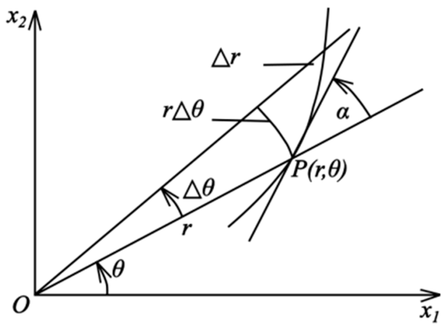
There are more qualitative properties of the LSP other than the index. For a linear velocity field, the isotropic points, whether center, focus, or node, have the same index, but possess different features depending on the eigenvalue structure or real Schur form. Thus, we may determine the answers to the following questions (among others): How do the streamlines pass through the isotropic point? Are the directions of these streamlines entering the isotropic point the same (tangent to each other)? Is there a streamline tangent to the circle centered at the isotropic point? The LSP would become more complex when the effect of nonlinear terms is considered. On the other hand, the qualitative properties can be identified from the types of curvilinear sectors, each of which is divided by two characteristic directions (CDs, or half-lines) starting from the isotropic point, and the relative positions of these sectors [14]. It should be pointed out that a streamline tending to the origin must tend to it either spirally or along a CD [14]. Except for the center and focus types, there are at least two CDs defined by

$${\displaystyle \frac{d\theta }{dt}}={\displaystyle \frac{x_1{v}_2-x_2{v}_1}{r^2}}=0,$$

(6)

or, equivalently,

$$\mathrm{t}\mathrm{a}\mathrm{n}\alpha ={\displaystyle \frac{rd\theta }{dr}}={\displaystyle \frac{x_1{v}_2-x_2{v}_1}{x_1{v}_1+x_2{v}_2}}={\displaystyle \frac{I\left(r,\theta \right)}{M\left(r,\theta \right)}}={\displaystyle \frac{G\left(\theta \right)+o\left(1\right)}{A\left(r,\theta \right)}}=0,$$

(7)

where the direction angle $\theta$ comes from $z=x_1+i{x}_2=r{e}^{i\theta }$ with $i=\sqrt{-1}$, and $\alpha$ is the angle between the radius vector and the velocity at the point $P(r, \theta )$, as shown in Figure 1. If there exist $\delta >0, K>0$ such that $\left|A\left(r,\theta \right)\right|<K$ for $r<\delta$, then $G\left({\theta }_c\right)=0$ is a necessary condition for $\theta ={\theta }_c$ to be a characteristic line. Let $P_m\left(x_1,x_2\right)=r^m{X}_m\left(\mathrm{c}\mathrm{o}\mathrm{s}\theta ,\mathrm{s}\mathrm{i}\mathrm{n}\theta \right)$ and $Q_n\left(x_1,x_2\right)=r^n{Y}_n\left(\mathrm{c}\mathrm{o}\mathrm{s}\theta ,\mathrm{s}\mathrm{i}\mathrm{n}\theta \right)$; thus, the function $G\left(\theta \right)$ is defined as

$$G\left(\theta \right)=\left\{\begin{array}{cc}\mathrm{c}\mathrm{o}\mathrm{s}\theta Y_n\left(\mathrm{c}\mathrm{o}\mathrm{s}\theta ,\mathrm{s}\mathrm{i}\mathrm{n}\theta \right)& ,m>n\\ {-\mathrm{s}\mathrm{i}\mathrm{n}\theta X}_m\left(\mathrm{c}\mathrm{o}\mathrm{s}\theta ,\mathrm{s}\mathrm{i}\mathrm{n}\theta \right)& ,m<n\\ \mathrm{c}\mathrm{o}\mathrm{s}\theta Y_n\left(\mathrm{c}\mathrm{o}\mathrm{s}\theta ,\mathrm{s}\mathrm{i}\mathrm{n}\theta \right){-\mathrm{s}\mathrm{i}\mathrm{n}\theta X}_m\left(\mathrm{c}\mathrm{o}\mathrm{s}\theta ,\mathrm{s}\mathrm{i}\mathrm{n}\theta \right)& ,m=n\end{array}\right..$$

(8)

The equation $G\left(\theta \right)=0$ is called the characteristic equation of (2) [14,15]. By virtue of the property (5), the assumption $m\le n$ is always valid.

For the isotropic point of an analytic vector field other than a center or a focus, when $\delta$ is small enough, there are no more than three kinds of sectors in the neighborhood bounded by the circle $\mathsf{\ell }=\left\{z:\left|z\right|=\delta \right\}$: parabolic, hyperbolic, and elliptic [16]. This is shown in Figure 2. The numbers of different sectors satisfy the Bendixson formula:

$$\mathrm{I}\mathrm{n}\mathrm{d}\left(\mathit{v},\mathsf{\ell }\right)=1+{\displaystyle \frac{e-h}{2}},$$

(9)

where $e,h$ are the numbers of elliptic and hyperbolic sectors, respectively.

The analysis of LSP, namely the sector analysis, can be carried out using the following steps: (1) find out all CDs (if there are no CDs, the isotropic point is a center or a focus); (2) determine the type of sectors between adjacent CDs; (3) judge the entry direction of streamlines in a parabolic sector tending to the isotropic point. Usually, the separatrix is a radial half-line defined by $\theta ={\theta }_c$, and its direction is independent of the radial position. However, when the lower order terms cannot determine the isolated singular point, the separatrix may not be a radial line. Once the separatrices are confirmed, we can identify the flow directions on them by the signs of

$${\displaystyle \frac{d\mathrm{l}\mathrm{n}r}{dt}}={\displaystyle \frac{x_1{v}_1+x_2{v}_2}{r^2}}.$$

(10)

The streamline leaves the singularity when ${\displaystyle \frac{d\mathrm{l}\mathrm{n}r}{dt}}>0$, or enters when ${\displaystyle \frac{d\mathrm{l}\mathrm{n}r}{dt}}<0$. Next, we can judge the sector to be parabolic if its two separatrices, defined by angles ${\theta }_{c1}$ and ${\theta }_{c2}$ where $2\pi >{\theta }_{c2}>{\theta }_{c1}\ge 0$ have the same streamline direction (Figure 2a); we then determine along which direction all streamlines in the sector tend to the isotropic point as $r\to 0^{+}$. If two separatrices of a sector have different streamline directions, e.g., ${\left.{\displaystyle \frac{d\mathrm{l}\mathrm{n}r}{dt}}\right|}_{{\theta }_{c1}}>0>{\left.{\displaystyle \frac{d\mathrm{l}\mathrm{n}r}{dt}}\right|}_{{\theta }_{c2}}$, then one can definitely find a tangent point of some streamline in the sector to the circle centered at the origin, namely ${\left.{\displaystyle \frac{d\mathrm{l}\mathrm{n}r}{dt}}\right|}_{\theta ={\theta }_t}=0$ with ${\theta }_t\in \left({\theta }_{c1},{\theta }_{c2}\right)$. A negative ${\left.{\displaystyle \frac{d\theta }{dt}}\right|}_{\theta ={\theta }_t^{+}}<0$ indicates a hyperbolic sector (Figure 2b), while a positive value indicates an elliptic sector (Figure 2c). From the sectors and their types, we can calculate the index by applying the Bendixson Formula (9).

The index of an isolated point can be used to build up a topological classification, and forms an important basis of streamline pattern, but this is not enough. Jiang and Llibre [17] proposed the qualitative equivalence of two isotropic points with the same index, where two streamlines start or end in the same direction at one isotropic point if, and only if, the two equivalent streamlines start or end in the same direction at the other isotropic point. For velocity fields with a nonzero linear part, they presented a well-studied classification to date with some parameters, such as the eigenvalues of the coefficient matrix of the linear part, and the leading term(s) of higher order. In fluid mechanics, most studies are limited to the non-degenerate velocity gradient, in which the coefficients of the characteristic equation [18] and the real Schur form [19] are used to identify the streamline pattern.

This paper introduces a novel classification of LSPs according to the invariance of the velocity field under transformations of time, coordinates, and velocity scaling, together with the consideration of definite geometric features in the streamline pattern.

For an analytic velocity field with a nonzero linear part in the neighborhood of an isotropic point, the following spatiotemporal transformations and the linear transformation of velocity may be considered:

(i)

The time transformation, $t\mapsto at (a\ne 0)$, means that the absolute direction and speed of velocity do not affect the LSP.

(ii)

The coordinate transformations, including the following:

(ii.1)

The non-degenerate linear transformation, $\left(\begin{array}{c}{x}_1\\ x_2\end{array}\right)\mapsto \mathit{A}\left(\begin{array}{c}{x}_1\\ x_2\end{array}\right)$, where $\mathit{A}=\left(\begin{array}{cc}{a}_{11}& a_{12}\\ a_{21}& a_{22}\end{array}\right),\mathrm{d}\mathrm{e}\mathrm{t}\mathit{A}\ne 0$. The transformation could be a rotation $\left(\begin{array}{cc}\mathrm{c}\mathrm{o}\mathrm{s}\varphi & \mathrm{s}\mathrm{i}\mathrm{n}\varphi \\ -\mathrm{s}\mathrm{i}\mathrm{n}\varphi & \mathrm{c}\mathrm{o}\mathrm{s}\varphi \end{array}\right)$, a deformation $\left(\begin{array}{cc}\mathrm{c}\mathrm{o}\mathrm{s}\phi & \mathrm{s}\mathrm{i}\mathrm{n}\phi \\ -\mathrm{s}\mathrm{i}\mathrm{n}\phi & \mathrm{c}\mathrm{o}\mathrm{s}\phi \end{array}\right)\left(\begin{array}{cc}\alpha & 0\\ 0& \beta \end{array}\right)\left(\begin{array}{cc}\mathrm{c}\mathrm{o}\mathrm{s}\phi & -\mathrm{s}\mathrm{i}\mathrm{n}\phi \\ \mathrm{s}\mathrm{i}\mathrm{n}\phi & \mathrm{c}\mathrm{o}\mathrm{s}\phi \end{array}\right)$ with $\alpha ,\beta >0$, a mirror $\left(\begin{array}{cc}1& 0\\ 0& -1\end{array}\right)$, or their combination; this means the affine transformation does not change the LSP, and the chirality will not be used to distinguish the LSP, i.e., the right spiral is equivalent to the left spiral.

(ii.2)

A kind of near-identity transformation [20,21], $\left(\begin{array}{c}{x}_1\\ x_2\end{array}\right)\mapsto \left(\begin{array}{c}{x}_1+h_1\left(x_1,x_2\right)\\ x_2+h_2\left(x_1,x_2\right)\end{array}\right)$, where $h_1\left(x_1,x_2\right), h_2\left(x_1,x_2\right)$ are undetermined higher polynomials used to eliminate the nonlinear terms in $v_1,v_2$, resulting in the normal form of velocity field. That means that all the nonlinear velocity fields with nonzero linear part are locally equivalent if they have the same normal form at the isotropic point.

(ii.3)

The blow-up transformation, $\left(\begin{array}{c}{x}_1\\ x_2\end{array}\right)\mapsto \left(\begin{array}{c}{x}_1\\ x_{1}u\end{array}\right),u\ne 0$. The idea behind the blow-up technique is to replace the plane with a surface and the singular point $p$ on the plane by a line or by a circle on the surface such that the singular point $p$ can be ideally split into a finite number of simpler singularities $p_i$ on the line or the circle [13].

(ii.4)

The positive power transformation: $\left(\begin{array}{c}{x}_1\\ x_2\end{array}\right)\mapsto \left(\begin{array}{c}{x}_1^a\\ x_2^b\end{array}\right)$ with $a, b>0$. The transformation will be specially applied to the hyperbolic sector, where the streamlines tending to the isotropic point are finite in number.

(iii)

The proper linear transformation of velocity, $\left(\begin{array}{c}{v}_1\\ v_2\end{array}\right)\mapsto \mathit{B}\left(\begin{array}{c}{v}_1\\ v_2\end{array}\right)$, $\mathit{B}=\left(\begin{array}{cc}{b}_{11}& b_{12}\\ b_{21}& b_{22}\end{array}\right)$ with $\mathrm{d}\mathrm{e}\mathrm{t}\mathit{B}>0$.

Applying these transformations to (1), we no longer need to distinguish attracting and repelling, left and right spirals, and expansion and compression. And for convenience, the nonzero expansion and compression parameters have no difference, and the nonzero rotation parameter can be normalized to one when no expansion/compression occurs. In general, the invariance under spatiotemporal transformations yields a kind of qualitative classification, while the invariance under all transformations results in the topological classification.

3. Re-Examination of the Classification of Linear Velocity Fields

Starting from the linear velocity field,

$$\left(\begin{array}{c}{\dot{x}}_1\\ {\dot{x}}_2\end{array}\right)=\left(\begin{array}{c}{v}_1\\ v_2\end{array}\right)=\mathit{D}\left(\begin{array}{c}{x}_1\\ x_2\end{array}\right),\mathit{D}=\left(\begin{array}{cc}{d}_{11}& d_{12}\\ d_{21}& d_{22}\end{array}\right),$$

(11)

we solve the characteristic equation $\left|\begin{array}{cc}{d}_{11}-\lambda & d_{12}\\ d_{21}& d_{22}-\lambda \end{array}\right|=0$ to obtain two real eigenvalues ${\lambda }_1,{\lambda }_2$ or a pair of complex eigenvalues $\vartheta \pm i\mu$, and use the corresponding eigenvectors to construct an affine transformation $\left(\begin{array}{c}{x}_1\\ x_2\end{array}\right)\mapsto \mathit{A}\left(\begin{array}{c}{x}_1\\ x_2\end{array}\right), \mathrm{d}\mathrm{e}\mathrm{t}\left(\mathit{A}\right)>0$, so that

$$\left(\begin{array}{c}{\dot{x}}_1\\ {\dot{x}}_2\end{array}\right)={\mathit{J}}_{\mathit{D}}\left(\begin{array}{c}{x}_1\\ x_2\end{array}\right)$$

(12)

with the Jordan matrix ${\mathit{J}}_{\mathit{D}}$ taking the form

$${\mathit{J}}_{\mathit{D}}=\left(\begin{array}{cc}{\lambda }_1& 0\\ 0& {\lambda }_2\end{array}\right) \mathrm{o}\mathrm{r} \left(\begin{array}{cc}\vartheta & \mu \\ -\mu & \vartheta \end{array}\right) \mathrm{o}\mathrm{r} \left(\begin{array}{cc}\vartheta & 1\\ 0& \vartheta \end{array}\right),$$

(13)

which can be applied to classify the LSP of linear velocity fields around the origin into six types [17]: (1) saddle if ${\lambda }_1{\lambda }_2<0$; (2) two-direction node if ${\lambda }_1{\lambda }_2>0$ and ${\lambda }_1\ne {\lambda }_2$; (3) star-like node if ${\lambda }_1={\lambda }_2$ and ${\mathit{J}}_{\mathit{D}}$ can be diagonalized; (4) one-direction node if ${\lambda }_1={\lambda }_2=\vartheta$ and ${\mathit{J}}_{\mathit{D}}$ cannot be diagonalized; (5) center if two eigenvalues are pure imaginary; (6) focus if two eigenvalues are complex with nonzero real part. For the cases of linear velocity fields with one or more zero eigenvalues, the origin is no longer an isolated singularity.

Recently, after a definite rotation, the real Schur form of $\mathit{D}$ ($\tau \omega \ge 0$)

$${\mathit{S}}_{\mathit{D}}=\mathit{R}\mathit{D}{\mathit{R}}^{\mathit{T}}=\left(\begin{array}{cc}\vartheta & \tau +\omega \\ \tau -\omega & \vartheta \end{array}\right), \mathit{R}\in \mathrm{S}\mathrm{O}\left(2\right)$$

(14)

is actively applied to work out some vortex criteria [19,22,23,24]. Defining $J_2=\mathrm{d}\mathrm{e}\mathrm{t}\left(\mathit{A}\right)={\lambda }_1{\lambda }_2={\vartheta }^2-{\tau }^2+{\omega }^2$, we can also build up the classification based on the parameter set $\left\{\vartheta , \tau ,\omega \right\}$, namely (1) saddle if $J_2<0$; (2) two-direction node if $J_2>0,$ ${\tau }^2\ne {\omega }^2$; (3) star-like node if $\vartheta \ne 0$ and $\tau =\omega =0$; (4) one-direction node if $\vartheta \ne 0$ and ${\tau }^2={\omega }^2\ne 0$; (5) center if $\vartheta =0, {\tau }^2<{\omega }^2$; (6) focus if $\vartheta \ne 0, {\tau }^2<{\omega }^2$.

The qualitative equivalence from the above two parameter systems is of algebraic nature [25], but somehow incompletely conclusive. People may split one pattern into more types through refined parameters or parameters of higher-order terms. For example, sometimes it is necessary to distinguish the expansion $\left(\begin{array}{cc}1& 0\\ 0& 1\end{array}\right)$ and the compression $\left(\begin{array}{cc}-1& 0\\ 0& -1\end{array}\right)$, the clockwise vortex $\left(\begin{array}{cc}0& -1\\ 1& 0\end{array}\right)$ and the counterclockwise one $\left(\begin{array}{cc}0& 1\\ -1& 0\end{array}\right)$, the left spiral $\left(\begin{array}{cc}1& -1\\ 1& 1\end{array}\right)$ and the right one $\left(\begin{array}{cc}1& 1\\ -1& 1\end{array}\right)$; it also needs to explain why $\left(\begin{array}{cc}1& 0\\ 0& -0.5\end{array}\right)$ and $\left(\begin{array}{cc}0& 1\\ 1& 0\end{array}\right)$ belong to the same type. In this paper, based on the common intuition about the classification of LSPs, we will adopt wider spatiotemporal coordinate transformations besides the usual scaling of time, space, and rotation. Space rotation is used to derive the real Schur form of the linear velocity field, while the deformation can be used to change the combination of $\tau$ and $\omega$ into a single $\tau$ if ${\tau }^2>{\omega }^2$; a single $\omega$ if ${\tau }^2<{\omega }^2$; or $\tau +\omega =\pm 1$ if ${\tau }^2={\omega }^2$. Time inversion and scaling can be used to normalize $\vartheta =1$, or $\omega =1$ if $\vartheta =\tau =0,$ or $\tau =1$ if $\vartheta =\omega =0.$ More transformations to be used for linear velocity fields include the following:

(i)

The mirror transformation to unify $\left(\begin{array}{cc}1& \omega \\ -\omega & 1\end{array}\right)$ and $\left(\begin{array}{cc}1& -\omega \\ \omega & 1\end{array}\right)$, $\left(\begin{array}{cc}1& 1\\ 0& 1\end{array}\right)$ and $\left(\begin{array}{cc}1& -1\\ 0& 1\end{array}\right)$;

(ii)

The positive power transformation to unify $\left(\begin{array}{cc}{\lambda }_1& 0\\ 0& {\lambda }_2\end{array}\right)$ with ${\lambda }_1{\lambda }_2<0$ and $\left(\begin{array}{cc}1& 0\\ 0& -1\end{array}\right)$.

Then, a complete standard form for linear velocity fields with $J_2\ne 0$, called the quasi-real Schur form under the spatiotemporal coordinate transformations, can be built up, as listed in

Table 1. Classification of elementary isotropic points.

Case	Determinant	Jordan Form	Real Schur Form	Quasi-Real Schur Form	Index	Sectors/ Separatrices	Type
1	$J_2<0$	${\lambda }_1>0>{\lambda }_2$	$\begin{array}{c}{\tau }^2-{\omega }^2\\ >{\vartheta }^2>0\end{array}$	$\left(\begin{array}{cc}1& 0\\ 0& -1\end{array}\right)$	$-1$	4/4	Saddle
2	$J_2>0$	${\lambda }_1>{\lambda }_2>0$	$\begin{array}{c}{\vartheta }^2>{\tau }^2\\ -{\omega }^2>0\end{array}$	$\begin{array}{c}\left(\begin{array}{cc}1+\tau & 0\\ 0& 1-\tau \end{array}\right),\\ \tau \in \left(\mathrm{0,1}\right)\end{array}$	1	4/4	Two-direction node
3		$\left(\begin{array}{cc}0& \mu \\ -\mu & 0\end{array}\right)$	$\begin{array}{c}\vartheta =0>\\ {\tau }^2-{\omega }^2\end{array}$	$\left(\begin{array}{cc}0& 1\\ -1& 0\end{array}\right)$	1	0/0	Vortex (center)
4		$\left(\begin{array}{cc}\vartheta & \mu \\ -\mu & \vartheta \end{array}\right)$	${\vartheta }^2>0>{\tau }^2-{\omega }^2$	$\begin{array}{c}\left(\begin{array}{cc}1& \omega \\ -\omega & 1\end{array}\right),\\ \omega >0\end{array}$	1	0/0	Spiral (focus)
5		$\left(\begin{array}{cc}\vartheta & 1\\ 0& \vartheta \end{array}\right)$	$\left(\begin{array}{cc}\vartheta & 2\tau \\ 0& \vartheta \end{array}\right)$	$\left(\begin{array}{cc}1& 1\\ 0& 1\end{array}\right)$	1	2/2	One-direction node
6		$\left(\begin{array}{cc}\vartheta & 0\\ 0& \vartheta \end{array}\right)$	$\left(\begin{array}{cc}\vartheta & 0\\ 0& \vartheta \end{array}\right)$	$\left(\begin{array}{cc}1& 0\\ 0& 1\end{array}\right)$	1	$\mathrm{\infty }/\mathrm{\infty }$	Star-like node
7	$J_2=0$	$\left(\begin{array}{cc}\lambda & 0\\ 0& 0\end{array}\right)$, $\left(\begin{array}{cc}0& 1\\ 0& 0\end{array}\right)$	$\left(\begin{array}{cc}\lambda & 0\\ 0& 0\end{array}\right)$, $\left(\begin{array}{cc}0& 2\tau \\ 0& 0\end{array}\right)$	$\left(\begin{array}{cc}1& 0\\ 0& 0\end{array}\right)$, $\left(\begin{array}{cc}0& 1\\ 0& 0\end{array}\right)$	-	-	Straight

.

Finally, for the topological equivalence, by applying the positive definite linear transformation to the linear velocity fields, we can merge different qualitative types into two classes: $\left(\begin{array}{cc}1& 0\\ 0& 1\end{array}\right)$ and $\left(\begin{array}{cc}1& 0\\ 0& -1\end{array}\right)$, with the index values $1$ and $-1$, respectively.

The classification of linear velocity fields can also be achieved directly from their explicit solutions. Substituting the quasi-real Schur form listed in Table 1 into (12), we derive the results as follows:

Case 1. Saddle, from

$${\displaystyle \frac{d\mathrm{l}\mathrm{n}r}{dt}}={\displaystyle \frac{x_1{v}_1+x_2{v}_2}{r^2}}=\mathrm{c}\mathrm{o}\mathrm{s}2\theta , {\displaystyle \frac{d\theta }{dt}}={\displaystyle \frac{x_1{v}_2-x_2{v}_1}{r^2}}=-\mathrm{s}\mathrm{i}\mathrm{n}2\theta ,$$

(15)

we obtain the analytic solution satisfying $r\left(0\right)=r_0, \theta \left(0\right)={\theta }_0$ to be

$$r\left(t\right)=r_0\sqrt{e^{2t}{{\mathrm{c}\mathrm{o}\mathrm{s}}^2{\theta }_0+e^{-2t}\mathrm{s}\mathrm{i}\mathrm{n}}^2{\theta }_0}, \theta \left(t\right)=\mathrm{a}\mathrm{r}\mathrm{c}\mathrm{t}\mathrm{a}\mathrm{n}\left(e^{-2t}\mathrm{t}\mathrm{a}\mathrm{n}{\theta }_0\right).$$

(16)

The qualitative properties following from (16) include the following: (1) the coordinate axes are streamlines and $\theta \left(t\to \pm \infty \right)\to \left(0^{+},{{\displaystyle \frac{\pi }{2}}}^{-}\right) \mathrm{o}\mathrm{r} \left({\pi }^{+}, {{\displaystyle \frac{3\pi }{2}}}^{-}\right) \mathrm{i}\mathrm{f} \mathrm{t}\mathrm{a}\mathrm{n}{\theta }_0>0$, $\theta \left(t\to \pm \infty \right)\to \left(0^{-},{{\displaystyle \frac{3\pi }{2}}}^{+}\right)$, or $\left({\pi }^{-}, {{\displaystyle \frac{\pi }{2}}}^{+}\right) \mathrm{i}\mathrm{f} \mathrm{t}\mathrm{a}\mathrm{n}{\theta }_0<0$, so there are four separatrices ${\theta }_c=0,{\displaystyle \frac{\pi }{2}}, {\displaystyle \frac{3\pi }{2}}, \pi$, and no other streamline enters the isotropic point, say if ${\theta }_0\ne {\theta }_c$, $r\to \infty$ when $t\to \pm \infty$; (2) for every circle centered at the origin, there are four points at ${\theta }_{1–4}={\displaystyle \frac{\pi }{4}},{\displaystyle \frac{3\pi }{4}},{\displaystyle \frac{5\pi }{4}},{\displaystyle \frac{7\pi }{4}}$, circumferential to four streamlines, respectively. The isotropic point with streamlines, except the separatrices which, being hyperbolic, is called a saddle, with the streamlines $x_1{x}_2=C$ and ${\mathrm{I}\mathrm{n}\mathrm{d}}_O=-1$ from (9).

Case 2. Two-direction node, from

$${\displaystyle \frac{d\mathrm{l}\mathrm{n}r}{dt}}=\left(1+\tau \right){\mathrm{c}\mathrm{o}\mathrm{s}}^2\theta +\left(1-\tau \right){\mathrm{s}\mathrm{i}\mathrm{n}}^2\theta , {\displaystyle \frac{d\theta }{dt}}=-\tau \mathrm{s}\mathrm{i}\mathrm{n}2\theta , \tau \in \left(\mathrm{0,1}\right),$$

(17)

we have

$$r\left(t\right)=r_0{e}^t\sqrt{e^{2\tau t}{{\mathrm{c}\mathrm{o}\mathrm{s}}^2{\theta }_0+e^{-2\tau t}\mathrm{s}\mathrm{i}\mathrm{n}}^2{\theta }_0}, \theta \left(t\right)=\mathrm{a}\mathrm{r}\mathrm{c}\mathrm{t}\mathrm{a}\mathrm{n}\left(e^{-2\tau t}\mathrm{t}\mathrm{a}\mathrm{n}{\theta }_0\right)$$

(18)

with the following qualitative properties: (1) the coordinate axes are streamlines, $\theta \left(t\to \pm \infty \right)\to \left(0^{+},{{\displaystyle \frac{\pi }{2}}}^{-}\right) \mathrm{o}\mathrm{r} \left({\pi }^{+}, {{\displaystyle \frac{3\pi }{2}}}^{-}\right) \mathrm{i}\mathrm{f} \mathrm{t}\mathrm{a}\mathrm{n}{\theta }_0>0, \theta \left(t\to \pm \infty \right)\to \left(0^{-},{{\displaystyle \frac{3\pi }{2}}}^{+}\right) \mathrm{o}\mathrm{r} \left({\pi }^{-}, {{\displaystyle \frac{\pi }{2}}}^{+}\right)$ if $\mathrm{t}\mathrm{a}\mathrm{n}{\theta }_0<0$, so there are four separatrices; (2) no streamline is tangent to the circle centered at the origin, the streamlines other than the separatrices enter the origin ($t\to -\infty$), and are tangent to radial lines with $\theta$ equal to ${\displaystyle \frac{\pi }{2}}$ or ${\displaystyle \frac{3\pi }{2}}$. The isotropic point with streamlines, except the separatrices, being parabolic is called a node, with the streamlines $x_2=C{x}_1^{{\displaystyle \frac{1+\tau }{1-\tau }}}$ and ${\mathrm{I}\mathrm{n}\mathrm{d}}_O=1$.

Case 3. Vortex, the explicit solution is simply $r\left(t\right)=r_0$ for streamline passing through $\left(r_0, {\theta }_0\right)$, all streamlines are circles except the center point, with the streamlines $x_1^2+x_2^2=C>0$, and ${\mathrm{I}\mathrm{n}\mathrm{d}}_O=1$ from the definition.

Case 4. Spiral, from

$${\displaystyle \frac{d\mathrm{l}\mathrm{n}r}{dt}}=1, {\displaystyle \frac{d\theta }{dt}}=-\omega ,$$

(19)

we get $r\left(t\right)=r_0{e}^t, \theta \left(t\right)={\theta }_0-\omega t$ for streamline passing through $\left(r_0, {\theta }_0\right)$, which means that there is no separatrix and all streamlines are helical starting from the origin, with the streamlines $\mathrm{l}\mathrm{n}{\left(x_1^2+x_2^2\right)}^{\omega }+\mathrm{a}\mathrm{r}\mathrm{c}\mathrm{t}\mathrm{a}\mathrm{n}\left({\displaystyle \frac{x_2}{x_1}}\right)=C$ and ${\mathrm{I}\mathrm{n}\mathrm{d}}_O=1$.

Case 5. One-direction node, from

$${\displaystyle \frac{d\mathrm{l}\mathrm{n}r}{dt}}=\left({\mathrm{c}\mathrm{o}\mathrm{s}}^2\theta +\mathrm{s}\mathrm{i}\mathrm{n}\theta \mathrm{c}\mathrm{o}\mathrm{s}\theta \right)+{\mathrm{s}\mathrm{i}\mathrm{n}}^2\theta =r\left(1+\mathrm{s}\mathrm{i}\mathrm{n}\theta \mathrm{c}\mathrm{o}\mathrm{s}\theta \right), {\displaystyle \frac{d\theta }{dt}}=-{\mathrm{s}\mathrm{i}\mathrm{n}}^2\theta ,$$

(20)

we have

$$r\left(t\right)=r_0\sqrt{{{\left(\mathrm{c}\mathrm{o}\mathrm{s}{\theta }_0+t\mathrm{s}\mathrm{i}\mathrm{n}{\theta }_0\right)}^2+\mathrm{s}\mathrm{i}\mathrm{n}}^2{\theta }_0}{e}^t, \theta \left(t\right)=\mathrm{a}\mathrm{r}\mathrm{c}\mathrm{t}\mathrm{a}\mathrm{n}\left({\displaystyle \frac{\mathrm{t}\mathrm{a}\mathrm{n}{\theta }_0}{1+t\mathrm{t}\mathrm{a}\mathrm{n}{\theta }_0}}\right).$$

(21)

The streamline pattern has the following properties: (1) only the $x_1$-axis forms two separatrices where $\theta \left(t\to -\infty \right)\to 0 \mathrm{o}\mathrm{r} \pi$; (2) no streamline is tangent to the circle centered at the origin; the streamlines other than the separatrices approach the origin ($t\to -\infty$), and are tangent to radial lines with $\theta$ equal to $0^{-} \mathrm{o}\mathrm{r} {\pi }^{-}$; (3) the velocity component $v_1$ changes its sign at the point on the line $x_1+x_2=0$. This streamline pattern is specially called a one-direction node, with the streamlines $x_1=x_2\left(\mathrm{l}\mathrm{n}\left|x_2\right|+C\right)$ and ${\mathrm{I}\mathrm{n}\mathrm{d}}_O=1$.

Case 6. Star-like node, the explicit solution is simply $\theta \left(t\right)={\theta }_0$, all streamlines $x_2=C{x}_1$ start from the origin ($t\to -\infty$).

Case 7. Undefined, the singular point is not isolated, and the streamlines $x_2=C$ are straight.

We summarize the analysis process as follows: (1) determine the separatrices, which means ${\displaystyle \frac{d\theta }{dt}}=0$ but ${\displaystyle \frac{dr}{dt}}\ne 0$ when $r\ne 0$; (2) find out whether the directions of flow in two adjacent separatrices are the same (both of them are inflow/outflow the isotropic point) or different (for the former, the sector is parabolic); (3) for the latter, find out the tangency of streamline with a circle centered at the isotropic point, if the tangency is external, the sector is hyperbolic, and otherwise, it is elliptic. Besides the above situations, the cases without separatrices are center-like, namely, the isotropic point is a center if the streamline is circular and otherwise, it is a spiral; for node cases, the number of separatrices and the entry way of streamlines approaching the isotropic point can be used to build up the classification. In fluid mechanics, both centers and foci are categorized as vortices, differing in that centers typically occur in 2D incompressible flows while foci do not. Nodes (encompassing one-direction, two-direction, and star-like nodes) and saddles correspond to fluid sources/sinks and attachment/separation points, respectively.

4. Classification of Nonlinear Velocity Fields with a Nonzero Linear Part

Assume that under the transformation $\left(\begin{array}{c}{x}_1\\ x_2\end{array}\right)\mapsto \mathit{A}\left(\begin{array}{c}{x}_1\\ x_2\end{array}\right)$, Equation (1) is transformed to coordinates corresponding to eigenvalues ${\lambda }_1,{\lambda }_2$ (which could be complex here), we have

$$\left(\begin{array}{c}{\dot{x}}_1\\ {\dot{x}}_2\end{array}\right)=\left(\begin{array}{cc}{\lambda }_1& 0\\ 0& {\lambda }_2\end{array}\right)\left(\begin{array}{c}{x}_1\\ x_2\end{array}\right)+\left(\begin{array}{ccccc}{c}_1^{N,0}& \cdots & c_1^{m_1,m_2}& \cdots & c_1^{0,N}\\ c_2^{N,0}& \cdots & c_2^{m_1,m_2}& \cdots & c_2^{0,N}\end{array}\right)\left(\begin{array}{c}{x}_1^N\\ ⋮\\ x_1^{m_1}{x}_2^{m_2}\\ ⋮\\ x_2^N\end{array}\right)+o\left(r^N\right), N>1.$$

(22)

According to the Poincaré–Dulac theorem, we can introduce a near-identity transformation [21] or a formal diffeomorphism [20]:

$$\left(\begin{array}{c}{x}_1\\ x_2\end{array}\right)\mapsto \left(\begin{array}{c}{x}_1\\ x_2\end{array}\right)+\left(\begin{array}{ccccc}{s}_1^{N,0}& \cdots & s_1^{m_1,m_2}& \cdots & s_1^{0,N}\\ s_2^{N,0}& \cdots & s_2^{m_1,m_2}& \cdots & s_2^{0,N}\end{array}\right)\left(\begin{array}{c}{x}_1^N\\ ⋮\\ x_1^{m_1}{x}_2^{m_2}\\ ⋮\\ x_2^N\end{array}\right)$$

(23)

to eliminate the nonlinear terms $c_i^{m_1,m_2}, i=\mathrm{1,2}$, by setting

$$s_i^{m_1,m_2}={\displaystyle \frac{c_i^{m_1,m_2}}{m_1{\lambda }_1+m_2{\lambda }_2-{\lambda }_i}}$$

(24)

if $m_1{\lambda }_1+m_2{\lambda }_2-{\lambda }_i\ne 0$; this process can continue for the next higher order part, and so on. The terms $x_1^{m_1}{x}_2^{m_2}$ with indices satisfying $m_1{\lambda }_1+m_2{\lambda }_2={\lambda }_i$ are called resonant with the linear part, and must be retained for inspection. The nonlinear Equation (22) without non-resonant terms is called the normal form of the velocity field with such a type of linear part [20]. Besides the above general derivation, we detail the cases with zero eigenvalues as follows.

The case with one eigenvalue being zero is called semi-elementary. Assuming that all terms with powers less than $N$ have been simplified to be of normal form, we begin to simplify the terms of order $N$ from the following expression:

$$\left(\begin{array}{c}{\dot{x}}_1\\ {\dot{x}}_2\end{array}\right)=\left(\begin{array}{cc}1& 0\\ 0& 0\end{array}\right)\left(\begin{array}{c}{x}_1\\ x_2\end{array}\right)+{\sum }_{1<k<N}\left(\begin{array}{c}{g}_1^k\left(x_1,x_2\right)\\ g_2^k\left(x_1,x_2\right)\end{array}\right)+\left(\begin{array}{c}{p}_1^N\left(x_1,x_2\right)\\ p_2^N\left(x_1,x_2\right)\end{array}\right)+o\left(r^N\right).$$

(25)

Making use of the transformation

$$\left(\begin{array}{c}{x}_1\\ x_2\end{array}\right)\mapsto \left(\begin{array}{c}{x}_1\\ x_2\end{array}\right)+\left(\begin{array}{c}{h}_1^N\left(x_1,x_2\right)\\ h_2^N\left(x_1,x_2\right)\end{array}\right),$$

(26)

substituting it into (25) yields

$$\left[\left(\begin{array}{cc}1& 0\\ 0& 1\end{array}\right)+\left(\begin{array}{cc}{\partial }_1{h}_1^N& {\partial }_2{h}_1^N\\ {\partial }_1{h}_2^N& {\partial }_2{h}_2^N\end{array}\right)\right]\left(\begin{array}{c}{\dot{x}}_1\\ {\dot{x}}_2\end{array}\right)=\left(\begin{array}{cc}1& 0\\ 0& 0\end{array}\right)\left(\begin{array}{c}{x}_1+h_1^N\\ x_2+h_2^N\end{array}\right)+{\sum }_{1<k<n}\left(\begin{array}{c}{g}_1^k\\ g_2^k\end{array}\right)+\left(\begin{array}{c}{p}_1^N\\ p_2^N\end{array}\right)+o\left(r^N\right).$$

(27)

Due to

$${\left[\left(\begin{array}{cc}1& 0\\ 0& 1\end{array}\right)+\left(\begin{array}{cc}{\partial }_1{h}_1^N& {\partial }_2{h}_1^N\\ {\partial }_1{h}_2^N& {\partial }_2{h}_2^N\end{array}\right)\right]}^{-1}=\left(\begin{array}{cc}1& 0\\ 0& 1\end{array}\right)-\left(\begin{array}{cc}{\partial }_1{h}_1^N& {\partial }_2{h}_1^N\\ {\partial }_1{h}_2^N& {\partial }_2{h}_2^N\end{array}\right)+o\left(r^{2N-2}\right)$$

(28)

and $2N-2\ge N$, we have

$$\left(\begin{array}{c}{\dot{x}}_1\\ {\dot{x}}_2\end{array}\right)=\left(\begin{array}{cc}1& 0\\ 0& 0\end{array}\right)\left(\begin{array}{c}{x}_1\\ x_2\end{array}\right)-\left(\begin{array}{cc}{\partial }_1{h}_1^N& {\partial }_2{h}_1^N\\ {\partial }_1{h}_2^N& {\partial }_2{h}_2^N\end{array}\right)\left(\begin{array}{cc}1& 0\\ 0& 0\end{array}\right)\left(\begin{array}{c}{x}_1\\ x_2\end{array}\right)+{\sum }_{1<k<N}\left(\begin{array}{c}{g}_1^k\\ g_2^k\end{array}\right)+\left(\begin{array}{c}{p}_1^N+h_1^N\\ p_2^N\end{array}\right)+o\left(r^N\right),$$

(29)

and so, the simplification of order $N$ does not affect the terms with orders less than $N$, and vice versa. The route of simplification is

$$p_1^N+h_1^N-x_1{\partial }_1{h}_1^N\to g_1^N, p_2^N-x_1{\partial }_1{h}_2^N\to g_2^N.$$

(30)

Hence, the terms in $\left(\begin{array}{c}{p}_1^N\\ p_2^N\end{array}\right)$ that cannot be eliminated from any Nth-order homogeneous polynomials $\left(\begin{array}{c}{h}_1^N\\ h_2^N\end{array}\right)$ are

$$g_1^N=a_{1,N-1}^N{x}_1{x}_2^{N-1}, g_2^N=a_{2,N}^N{x}_2^N,$$

(31)

and finally, the normal form of (25) is

$$\left(\begin{array}{c}{\dot{x}}_1\\ {\dot{x}}_2\end{array}\right)=\left(\begin{array}{c}{x}_1+x_1{\varphi }_1\left(x_2\right)\\ {\varphi }_2\left(x_2\right)\end{array}\right),$$

(32)

where ${\varphi }_1\left(x\right)$ is an arbitrary polynomial of order greater than 0, ${\varphi }_2\left(x\right)$ is an arbitrary polynomial of order greater than one.

The case with two eigenvalues being zero is called nilpotent. Similar derivation yields the following simplification relations

$$p_1^N+h_2^N-x_2{\partial }_1{h}_1^N\to g_1^N, p_2^N-x_2{\partial }_1{h}_2^N\to g_2^N,$$

(33)

which result in normal form

$${\displaystyle \frac{d}{dt}}\left(\begin{array}{c}{x}_1\\ x_2\end{array}\right)=\left(\begin{array}{c}{x}_2\\ {\varphi }_2\left(x_1\right)+x_2{\varphi }_1\left(x_1\right)\end{array}\right).$$

(34)

It should be noted that the normal form (34) is not unique, and $\left(\begin{array}{c}{x}_2+x_1{\varphi }_1\left(x_1\right)\\ {\varphi }_2\left(x_1\right)\end{array}\right)$ is another choice [26].

The normal forms of all nonlinear velocity fields with a nonzero linear part are listed in

Table 2. Normal forms of velocity fields with nonzero linear part.

Determinant	Quasi-Real Schur Form	Index	Type	Resonant Terms
$J_2<0$	$\left(\begin{array}{cc}1& 0\\ 0& -1\end{array}\right)$	$-1$	Saddle	$\left(\begin{array}{c}{x}_1\varphi \left(x_1{x}_2\right)\\ x_2{\varphi }_1\left(x_1{x}_2\right)\end{array}\right)$
$J_2>0$	$\left(\begin{array}{cc}1+\tau & 0\\ 0& 1-\tau \end{array}\right), \tau ={\displaystyle \frac{n-1}{n+1}},$	1	Two-direction node	$- \mathrm{o}\mathrm{r} \left(\begin{array}{c}a{x}_2^n\\ 0\end{array}\right)$
	$\left(\begin{array}{cc}0& 1\\ -1& 0\end{array}\right)$	1	Vortex or spiral	$\varphi \left(r^2\right)\left(\begin{array}{c}{x}_1\\ x_2\end{array}\right)$
	$\left(\begin{array}{cc}1& \omega \\ -\omega & 1\end{array}\right), \omega >0$	1	Spiral	-
	$\left(\begin{array}{cc}1& 1\\ 0& 1\end{array}\right)$	1	One-direction node	-
	$\left(\begin{array}{cc}1& 0\\ 0& 1\end{array}\right)$	1	Star-like node	-
$J_2=0$	$\left(\begin{array}{cc}1& 0\\ 0& 0\end{array}\right)$	-	?	$\left(\begin{array}{c}{x}_1{\varphi }_1\left(x_2\right)\\ {\varphi }_2\left(x_2\right)\end{array}\right)$
	$\left(\begin{array}{cc}0& 1\\ 0& 0\end{array}\right)$	-	?	$\left(\begin{array}{c}0\\ {\varphi }_2\left(x_1\right)+x_2 {\varphi }_1\left(x_1\right)\end{array}\right)$

Note: $a$ are real constant, $\varphi \left(x\right), {\varphi }_1\left(x\right)$ indicate any two polynomials without constant term, while ${\varphi }_2\left(x\right)$ is a polynomial of orders no less than 2.

. For the saddle type, the amplitudes of two eigenvalues of different signs could be adjusted by the positive power transformation, but do not affect the streamline pattern, and Zhang [14] also proved that the additional resonant terms of higher order will not change the topological or qualitative structures of velocity fields near the isotropic point when their linear parts have eigenvalues with nonzero real part. Thus, the complexity mainly comes from the cases of semi-elementary and nilpotent velocity fields with $J_2=0$, which will be discussed in the following. For the semi-elementary case with a zero eigenvalue, since the positive cofactor of velocity components can be merged with time, the normal form equation

$${\dot{x}}_1=x_1\left[1+{\varphi }_1\left(x_2\right)\right], {\dot{x}}_2={\varphi }_2\left(x_2\right)$$

(35)

is qualitatively equivalent to

$${\dot{x}}_1=x_1, {\dot{x}}_2={\displaystyle \frac{{\varphi }_2\left(x_2\right)}{1+{\varphi }_1\left(x_2\right)}}={\varphi }_2^{\prime }\left(x_2\right)=a{x}_2^m+o\left(x_2^m\right) ~a{x}_2^m, a\ne 0$$

(36)

in a small neighborhood of the origin, where $1+{\varphi }_1\left(x_2\right)$ is always larger than zero. Making use of a scaling transformation (plus a rotation by 180 degrees if $c<0$)

$$x_1\to c{x}_1, x_2\to c{x}_2, c=\left\{\begin{array}{cc}{a}^{1-m}& ,m \mathrm{i}\mathrm{s} \mathrm{e}\mathrm{v}\mathrm{e}\mathrm{n}, \\ {\left|a\right|}^{1-m}& , m \mathrm{i}\mathrm{s} \mathrm{o}\mathrm{d}\mathrm{d},\end{array}\right.$$

(37)

we can simplify (35) to

$${\dot{x}}_1=x_1, {\dot{x}}_2=\delta x_2^m, \delta =\left\{\begin{array}{cc}1& ,m \mathrm{i}\mathrm{s} \mathrm{e}\mathrm{v}\mathrm{e}\mathrm{n}, \\ \pm 1& ,m \mathrm{i}\mathrm{s} \mathrm{o}\mathrm{d}\mathrm{d}.\end{array}\right.$$

(38)

Then, the LSP of an isotropic point can be determined by the sign of $a$ and the parity of $m$ [14], as shown in Figure 3. Then, it becomes difficult to solve the following equations:

$$\begin{gathered} {\displaystyle \frac{d\mathrm{l}\mathrm{n}r}{dt}}=x_1{v}_1+x_2{v}_2={\mathrm{c}\mathrm{o}\mathrm{s}}^2\theta +\delta r^{m-1}{\mathrm{s}\mathrm{i}\mathrm{n}}^{m+1}\theta , \\ {\displaystyle \frac{d\theta }{dt}}={\displaystyle \frac{x_1{v}_2-x_2{v}_1}{r^2}}=\left(\delta r^{m-1}{\mathrm{s}\mathrm{i}\mathrm{n}}^{m-1}\theta -1\right)\mathrm{s}\mathrm{i}\mathrm{n}\theta \mathrm{c}\mathrm{o}\mathrm{s}\theta , \end{gathered}$$

(39)

but for a small enough $r$, we know that ${\displaystyle \frac{d\theta }{dt}}=0$ will give four separatrices ${\theta }_{1–4}=0,{\displaystyle \frac{\pi }{2}},\pi ,{\displaystyle \frac{3\pi }{2}}$, and so there are four sectors $s_{1–4}$ consecutively divided by the separatrices ${\theta }_1-{\theta }_2-{\theta }_3-{\theta }_4-{\theta }_1$. The flow directions of streamlines at ${\theta }_{\mathrm{2,4}}={\displaystyle \frac{\pi }{2}},{\displaystyle \frac{3\pi }{2}}$ are determined by $\delta$ and $m$: (1) for $m$ being even, the separatrix $x_1=0, x_2>0$ is expansive, $s_1$ and $s_2$ are parabolic with starting streamlines tangent to the separatrix $x_1=0,x_2>0$, the isotropic point is called a saddle–node (Figure 3a); (2) for $m$ being odd, all four sectors are parabolic with streamlines tangent to $x_2$-axis at the origin when $\delta =1$, or hyperbolic when $\delta =-1$, the isotropic point is called a node (Figure 3b) or a saddle (Figure 3c).

From the explicit solution $x_1=x_{10}{e}^{{\displaystyle \frac{1}{\left(m-1\right)\delta }}\left({\displaystyle \frac{1}{x_{20}^{m-1}}}-{\displaystyle \frac{1}{x_2^{m-1}}}\right)}$ of streamline passing through $\left(x_{10},x_{20}\right)$, we have

$${\displaystyle \frac{d{x}_1}{d{x}_2}}=x_{10}{e}^{{\displaystyle \frac{1}{\left(m-1\right)\delta x_{20}^{m-1}}}}{\left[\delta x_2^m{e}^{{\displaystyle \frac{1}{\left(m-1\right)\delta x_2^{m-1}}}}\right]}^{-1},$$

(40)

For $\delta =1$, since

$$\underset{x_2\to 0}{\lim }{x}_2^m{e}^{{\displaystyle \frac{1}{\left(m-1\right)x_2^{m-1}}}}\to +\infty ·\mathrm{s}\mathrm{i}\mathrm{g}\mathrm{n}\left(x_2\right) \mathrm{f}\mathrm{o}\mathrm{r} m=\mathrm{o}\mathrm{d}\mathrm{d} \mathrm{a}\mathrm{n}\mathrm{d} \underset{x_2\to 0^{+}}{\lim }{x}_2^m{e}^{{\displaystyle \frac{1}{\left(m-1\right)x_2^{m-1}}}}\to +\infty \mathrm{f}\mathrm{o}\mathrm{r} m=\mathrm{e}\mathrm{v}\mathrm{e}\mathrm{n},$$

it is easy to prove that the streamlines are tangent to $x_2$-axis when the sectors are parabolic ($\delta =1$). An interesting property of the hyperbolic sectors is the asymptotic behavior of streamlines as $x_2\to \pm \infty$: it is obvious that all streamlines have asymptotic slope ${\left.{\displaystyle \frac{d{x}_1}{d{x}_2}}\right|}_{x_2\to \pm \infty }\to 0$, but $x_1\to x_{10}{e}^{{\displaystyle \frac{1}{\left(m-1\right)\delta x_{20}^{m-1}}}}\ne 0$.

For the nilpotent case, Equation (1) becomes

$${\dot{x}}_1=x_2, {\dot{x}}_2={\varphi }_2\left(x_1\right)+x_2{\varphi }_1\left(x_1\right)=a{x}_1^p+b{x}_1^q{x}_2+o\left(x_1^p+x_1^q{x}_2\right) , a\ne 0, p>1,q>0.$$

(41)

Similar transformations to (37) can simplify (41) to

$${\dot{x}}_1=x_2, {\dot{x}}_2=\delta x_1^p+b{x}_1^q{x}_2, \delta =\left\{\begin{array}{cc}1& ,p \mathrm{i}\mathrm{s} \mathrm{e}\mathrm{v}\mathrm{e}\mathrm{n}, \\ \pm 1& , p \mathrm{i}\mathrm{s} \mathrm{o}\mathrm{d}\mathrm{d}.\end{array}\right.$$

(42)

For (42), making use of the transformations $\left(\begin{array}{c}{x}_1\\ x_2\end{array}\right)⟼\left(\begin{array}{cc}1& 0\\ 0& -1\end{array}\right)\left(\begin{array}{c}{x}_1\\ x_2\end{array}\right),t\to -t,$ we know that the sign of $b$ does not affect the LSP. Furthermore, the parameter value $b=1$ can always be achieved by the transformations such that $\left(\begin{array}{c}{x}_1\\ x_2\end{array}\right)⟼\left(\begin{array}{cc}{b}^{{\displaystyle \frac{2}{p-(2q+1)}}}& 0\\ 0& b^{{\displaystyle \frac{p+1}{p-(2q+1)}}}\end{array}\right)\left(\begin{array}{c}{x}_1\\ x_2\end{array}\right)$, $t\to b^{{\displaystyle \frac{1-p}{p-(2q+1)}}}t$ if $p\ne 2q+1$ and $b\ne 0$. Without loss of generality, we will take $b\ge 0$.

From

$${\displaystyle \frac{d\theta }{dt}}={\displaystyle \frac{x_1{v}_2-x_2{v}_1}{r^2}}=\left(\delta r^{p-1}{\mathrm{c}\mathrm{o}\mathrm{s}}^{p+1}\theta +b{r}^q\mathrm{s}\mathrm{i}\mathrm{n}\theta {\mathrm{c}\mathrm{o}\mathrm{s}}^{q+1}\theta -{\mathrm{s}\mathrm{i}\mathrm{n}}^2\theta \right),$$

(43)

we cannot determine any separatrix directly from the velocity field. Zhang [14] studied this class of Equations (42) by the blow-up technique, which originates from Poincaré, to decompose the nilpotent isotropic point into several elementary isotropic points, and concluded that the properties of the isotropic point will be determined by the size between $p \mathrm{a}\mathrm{n}\mathrm{d} 2q+1$, the parity of $p$ and $q$, the sign of $\delta$ and the sign of $∆=b^2+4\delta \left(q+1\right)$ for $p=2q+1$. Using the polar blow-up,

$$\begin{gathered} x_1=r\mathrm{c}\mathrm{o}\mathrm{s}\theta \mapsto r^{\alpha +1}\mathrm{c}\mathrm{o}\mathrm{s}\theta =r^{\alpha }{x}_1, x_2=r\mathrm{s}\mathrm{i}\mathrm{n}\theta \mapsto r^{\beta +1}\mathrm{s}\mathrm{i}\mathrm{n}\theta =r^{\beta }{x}_2, \\ dt=r^{\beta -\alpha -2}\left(r^2+\alpha x_1^2+\beta x_2^2\right)d\tau , \end{gathered}$$

(44)

where the minimal values of powers $\alpha$ and $\beta$ will be introduced to consider the higher-order effect, we obtain the following equations

$$\begin{gathered} {\displaystyle \frac{d{x}_1}{dt}}={\displaystyle \frac{r^{\beta -\alpha }\left(r^2+\beta x_2^2\right)-\alpha \delta r^{\alpha p-\beta }{x}_1^{p+1}-\alpha b{r}^{\alpha q}{x}_1^{q+1}{x}_2}{r^2+\alpha x_1^2+\beta x_2^2}}{x}_2, \\ {\displaystyle \frac{d{x}_2}{dt}}={\displaystyle \frac{\left(\delta r^{\alpha p-\beta }{x}_1^{p-1}+b{r}^{\alpha q}{x}_1^{q-1}{x}_2\right)\left(r^2+\alpha x_1^2\right)-\beta r^{\beta -\alpha }{x}_2^2}{r^2+\alpha x_1^2+\beta x_2^2}}{x}_1; \end{gathered}$$

(45)

and

$$\begin{gathered} {\displaystyle \frac{d\theta }{d\tau }}=\left(1+\alpha \right)\left(\delta r^{\left(\alpha +1\right)\left(p+1\right)-2\left(\beta +1\right)}{\mathrm{c}\mathrm{o}\mathrm{s}}^{p+1}\theta +b{r}^{\left(\alpha +1\right)\left(q+1\right)-\left(\beta +1\right)}{\mathrm{c}\mathrm{o}\mathrm{s}}^{q+1}\theta \mathrm{s}\mathrm{i}\mathrm{n}\theta \right)-\left(1+\beta \right){\mathrm{s}\mathrm{i}\mathrm{n}}^2\theta , \\ {\displaystyle \frac{d\mathrm{l}\mathrm{n}r}{d\tau }}=\left(1+\delta r^{\left(\alpha +1\right)\left(p+1\right)-2\left(\beta +1\right)}{\mathrm{c}\mathrm{o}\mathrm{s}}^{p-1}\theta +b{r}^{\left(\alpha +1\right)\left(q+1\right)-\left(\beta +1\right)}{\mathrm{c}\mathrm{o}\mathrm{s}}^{q-1}\theta \mathrm{s}\mathrm{i}\mathrm{n}\theta \right)\mathrm{c}\mathrm{o}\mathrm{s}\theta \mathrm{s}\mathrm{i}\mathrm{n}\theta . \end{gathered}$$

(46)

It is obvious that, just when $p=2q+1$, the complete exponent balance of terms with $\delta$ and $b$ as their coefficients is available; otherwise, only one of them ($\delta$ and $b$) balances with the other term, and we find the zeros by letting $r=0$ and determining the entry way of streamlines in a parabolic sector; this is determined by two CDs (${\theta }_{p1}$ and ${\theta }_{p2}(>{\theta }_{p1})$) approaching the isotropic point. Zhang [14] further pointed out that, in a small neighborhood of the origin, any streamline of (42) must tend to the origin spirally or along a fixed direction. The streamline is tangent to ${\theta }_{p1}$ or ${\theta }_{p2}$, depending on whether there is a direction ${\theta }_{*}\in \left({\theta }_{p1},{\theta }_{p2}\right)$, satisfying

$${\left.{\displaystyle \frac{d\theta }{d\tau }}\right|}_{\left(r,\theta \right)=\left(0,{\theta }_{*}\right)}·{\left.{\displaystyle \frac{d\mathrm{l}\mathrm{n}r}{d\tau }}\right|}_{\left(r,\theta \right)=\left(0,{\theta }_{p1}\right)}>0 \mathrm{o}\mathrm{r} {\left.{\displaystyle \frac{d\theta }{d\tau }}\right|}_{\left(r,\theta \right)=\left(0,{\theta }_{*}\right)}·{\left.{\displaystyle \frac{d\mathrm{l}\mathrm{n}r}{d\tau }}\right|}_{\left(r,\theta \right)=\left(0,{\theta }_{p2}\right)}<0,$$

(47)

which indicates that both the circumferential streamline $r\to 0, \theta \in \left({\theta }_{p1},{\theta }_{p2}\right)$ and the streamline $\theta ={\theta }_{p1}$ flow in or out of the point $\left(r,\theta \right)=(0,{\theta }_{p1})$, or one of the circumferential streamlines $r=0, \theta \in \left({\theta }_{p1},{\theta }_{p2}\right)$ and the streamline $\theta ={\theta }_{p2}$ flows in/out the point $(0,{\theta }_{p2})$. We will analyze the streamline pattern around the origin as follows.

Case 1: $b=0$ or $p<2q+1$. Then, we have $\left(\alpha +1\right)\left(q+1\right)-\left(\beta +1\right)>0$ when

$$\left(p+1\right)\left(\alpha +1\right)=2\left(\beta +1\right)\leftrightarrow \alpha =1,\beta =p,$$

(48)

and Equation (46) can be reduced to

$${\displaystyle \frac{d\theta }{d\tau }}=2\delta {\mathrm{c}\mathrm{o}\mathrm{s}}^{p+1}\theta -\left(p+1\right){\mathrm{s}\mathrm{i}\mathrm{n}}^2\theta , {\displaystyle \frac{d\mathrm{l}\mathrm{n}r}{d\tau }}=\left(1+\delta {\mathrm{c}\mathrm{o}\mathrm{s}}^{p-1}\theta \right)\mathrm{c}\mathrm{o}\mathrm{s}\theta \mathrm{s}\mathrm{i}\mathrm{n}\theta .$$

(49)

Case 1.1: when $p \mathrm{i}\mathrm{s} \mathrm{o}\mathrm{d}\mathrm{d}$ and $\delta =-1$, there is no separatrix and ${Ind}_O=1$ from (9) since $e=h=0$, indicating that the isotropic point is a center with streamlines $x_2^2+{\displaystyle \frac{1}{p+1}}{x}_1^{p+1}=0 \mathrm{i}\mathrm{f} b=0$, or a focus since ${\displaystyle \frac{\partial v_1}{\partial x_1}}+{\displaystyle \frac{\partial v_2}{\partial x_2}}=x_1^q\ne 0$ if $b\ne 0$.

Case 1.2: when $p \mathrm{i}\mathrm{s} \mathrm{o}\mathrm{d}\mathrm{d}$ and $\delta =1$, there are four separatrices from ${\mathrm{c}\mathrm{o}\mathrm{s}}^{\frac{p+1}{2}}\theta =\sqrt{{\displaystyle \frac{p+1}{2}}}\mathrm{s}\mathrm{i}\mathrm{n}\theta$ defined by $\theta ={\theta }_k\in \left(0,{\displaystyle \frac{\pi }{2}}\right), \pi -{\theta }_k, \pi +{\theta }_k, 2\pi -{\theta }_k$, in which the fluid flows out, in, out and in, respectively. All four sectors are hyperbolic since the streamlines are externally tangent to the circle centered at the origin. From (9), ${Ind}_O=-1$, and the isotropic point is a saddle.

Case 1.3: when $p \mathrm{i}\mathrm{s} \mathrm{e}\mathrm{v}\mathrm{e}\mathrm{n}\left(\delta =1\right)$, there are two non-collinear separatrices: $\theta ={\theta }_k\in \left(0,{\displaystyle \frac{\pi }{2}}\right), 2\pi -{\theta }_k$ where the streamlines flow out and in, respectively. According to the tangency and flow directions, the streamlines between the separatrices and around the origin can be illustrated by Figure 4a (right). This is a typical cusp with two hyperbolic sectors and so ${Ind}_O=0$.

Case 2: When $b\ne 0$, $p>2q+1$, we have $\left(\alpha +1\right)\left(p+1\right)-2\left(\beta +1\right)\left(\alpha +1\right)>0$ from $\left(\alpha +1\right)\left(q+1\right)-\left(\beta +1\right)=0$, and the parameters $\alpha =0,\beta =q$ reduce Equation (46) to be

$$\begin{gathered} {\displaystyle \frac{d\theta }{d\tau }}=\delta {r^{p-2q-1}\mathrm{c}\mathrm{o}\mathrm{s}}^{p+1}\theta +{\mathrm{c}\mathrm{o}\mathrm{s}}^{q+1}\theta \mathrm{s}\mathrm{i}\mathrm{n}\theta -\left(1+q\right){\mathrm{s}\mathrm{i}\mathrm{n}}^2\theta , \\ {\displaystyle \frac{d\mathrm{l}\mathrm{n}r}{d\tau }}=\left(1+\delta r^{p-2q-1}{\mathrm{c}\mathrm{o}\mathrm{s}}^{p-1}\theta +{\mathrm{c}\mathrm{o}\mathrm{s}}^{q-1}\theta \mathrm{s}\mathrm{i}\mathrm{n}\theta \right)\mathrm{c}\mathrm{o}\mathrm{s}\theta \mathrm{s}\mathrm{i}\mathrm{n}\theta . \end{gathered}$$

(50)

Here, we encounter a special situation in which the lower terms cannot make the origin an isolated singularity. By letting $r=0$, we obtain $\mathrm{s}\mathrm{i}\mathrm{n}\theta ={\displaystyle \frac{1}{q+1}}{\mathrm{c}\mathrm{o}\mathrm{s}}^{q+1}\theta$ and $\mathrm{s}\mathrm{i}\mathrm{n}\theta =0$ from ${\displaystyle \frac{d\theta }{d\tau }}=0$. The former really defines two separatrices, ${\theta }_{\mathrm{1,2}}$, but the latter also results in ${\displaystyle \frac{d\mathrm{l}\mathrm{n}r}{d\tau }}=0$, which comes from the cofactor $x_2$ that is not allowed. Starting from the point $r=0, \theta =0 \mathrm{o}\mathrm{r} \pi$, ${\theta }_{\mathrm{3,4}}^h$ involving higher-order terms, called the higher-order separatrix, must be introduced, the solutions ${\theta }^h\left(r\right)$ of $\delta {r^{p-2q-1}\mathrm{c}\mathrm{o}\mathrm{s}}^{p+1}{\theta }^h+{\mathrm{c}\mathrm{o}\mathrm{s}}^{q+1}{\theta }^h\mathrm{s}\mathrm{i}\mathrm{n}{\theta }^h-\left(1+q\right){\mathrm{s}\mathrm{i}\mathrm{n}}^2{\theta }^h=0$ with ${\theta }^h\left(r=0\right)=0 \mathrm{o}\mathrm{r} \pi$ yield two special separatrices.

Case 2.1: When $q \mathrm{i}\mathrm{s} \mathrm{o}\mathrm{d}\mathrm{d}$, we have two separatrices $\theta ={\theta }_{\mathrm{1,2}}$ lying in the quadrants I/II and two higher-order separatrices starting from $\left(r,\theta \right)=\left(0, 0\right)$ and $\left(0,\pi \right)$; there are tangency of streamlines to any circle centered at the origin at $\theta =0, {\displaystyle \frac{\pi }{2}},\pi , {\displaystyle \frac{3\pi }{2}}$, and the radial coordinate of streamlines increases in quadrants I/III and decreases in quadrants II/IV. These features mean that the isotropic point could be (1) saddle–node with ${Ind}_O=0$ if $p=\mathrm{e}\mathrm{v}\mathrm{e}\mathrm{n}$ and the streamlines in parabolic sectors are tangent to $\theta =\pi$ from (47); (2) elliptic–saddle with ${Ind}_O=1$ if $p=\mathrm{o}\mathrm{d}\mathrm{d},\delta =-1$ and all of the streamlines in one of the parabolic sectors are tangent to $\theta =0^{+}$ and the others are tangent to $\theta ={\pi }^{-}$; (3) saddle with ${Ind}_O=-1$ if $p=\mathrm{o}\mathrm{d}\mathrm{d},\delta =1$.

Case 2.2: When $q \mathrm{i}\mathrm{s} \mathrm{e}\mathrm{v}\mathrm{e}\mathrm{n}$, there are two separatrices $\theta ={\theta }_{\mathrm{1,2}}$ lying in the quadrants I/III. The isotropic point could be (1) saddle–node with ${Ind}_O=0$ if $p=\mathrm{e}\mathrm{v}\mathrm{e}\mathrm{n},$ and all of streamlines in parabolic sectors are tangent to $\theta =\pi$; (2) node with ${Ind}_O=1$ if $p=\mathrm{o}\mathrm{d}\mathrm{d},\delta =-1,$ and all of the streamlines in two parabolic sectors are tangent to $\theta =0$ and the others are tangent to $\theta =\pi$; (3) saddle with ${Ind}_O=-1$ if $p=\mathrm{o}\mathrm{d}\mathrm{d},\delta =1$.

Case 3: When $b\ne 0$, $p=2q+1$, we take

$$\left(p+1\right)\left(\alpha +1\right)=2\left(\beta +1\right)\leftrightarrow \alpha =0,\beta ={\displaystyle \frac{p-1}{2}}=q,$$

(51)

and thus obtain

$$\begin{gathered} {\displaystyle \frac{d\theta }{d\tau }}=\delta {\mathrm{c}\mathrm{o}\mathrm{s}}^{2q+2}\theta +b{\mathrm{c}\mathrm{o}\mathrm{s}}^{q+1}\theta \mathrm{s}\mathrm{i}\mathrm{n}\theta -\left(q+1\right){\mathrm{s}\mathrm{i}\mathrm{n}}^2\theta , \\ {\displaystyle \frac{d\mathrm{l}\mathrm{n}r}{d\tau }}=\left(1+\delta {\mathrm{c}\mathrm{o}\mathrm{s}}^{2q}\theta +b{\mathrm{c}\mathrm{o}\mathrm{s}}^{q-1}\theta \mathrm{s}\mathrm{i}\mathrm{n}\theta \right)\mathrm{c}\mathrm{o}\mathrm{s}\theta \mathrm{s}\mathrm{i}\mathrm{n}\theta . \end{gathered}$$

(52)

The structure of the quadratic form (52)₁ of ${\mathrm{c}\mathrm{o}\mathrm{s}}^{q+1}\theta$ and $\mathrm{s}\mathrm{i}\mathrm{n}\theta$ can be clarified by the following discriminant:

$$∆=b^2+4\delta \left(q+1\right).$$

(53)

Case 3.1: If $∆<0$, which is possible only when $\delta =-1$, then there is no separatrix, and the origin is a focus since ${\displaystyle \frac{\partial v_1}{\partial x_1}}+{\displaystyle \frac{\partial v_2}{\partial x_2}}=b{x}_1^q\ne 0$, and ${Ind}_O=1$.

Case 3.2: If $∆>0$, and $q \mathrm{i}\mathrm{s} \mathrm{o}\mathrm{d}\mathrm{d}$,$\delta =1$, then we obtain four separatrices ${\theta }_{1–4}$ in four quadrants from ${\mathrm{c}\mathrm{o}\mathrm{s}}^{q+1}\theta ={\mu }_k\mathrm{s}\mathrm{i}\mathrm{n}\theta ,k=\mathrm{1,2}, {\mu }_1{\mu }_2<0$, and can determine the origin being a saddle with ${Ind}_O=-1$ from the external tangency and flow directions.

Case 3.3: If $∆>0$, and $q \mathrm{i}\mathrm{s} \mathrm{o}\mathrm{d}\mathrm{d}$,$\delta =-1$, we have four non-collinear separatrices ${\theta }_{1-4}$ ($0<{\theta }_1<{\theta }_2<{\displaystyle \frac{\pi }{2}}<{\theta }_3<{\theta }_4<\pi$) from ${\mathrm{c}\mathrm{o}\mathrm{s}}^{q+1}\theta ={\mu }_i\mathrm{s}\mathrm{i}\mathrm{n}\theta$, ${\mu }_1,{\mu }_2>0$ since $b>0$. As shown in Figure 4b, one hyperbolic sector and an elliptic sector separated by two parabolic sectors yields an elliptic–saddle singularity with ${Ind}_O=1$; according to the criterion presented in (47), all the streamlines in one of parabolic sectors are tangent to $\theta ={\theta }_1^{+}$ and the others are tangent to $\theta ={\theta }_4^{-}$.

Case 3.4: If $∆>0$, and $q \mathrm{i}\mathrm{s} \mathrm{e}\mathrm{v}\mathrm{e}\mathrm{n}$, $\delta =1$, then we obtain a saddle with four separatrices in four quadrants, and ${Ind}_O=-1$.

Case 3.5: For $∆>0$, $q \mathrm{i}\mathrm{s} \mathrm{e}\mathrm{v}\mathrm{e}\mathrm{n}$, $\delta =-1$, we have four separatrices ${\theta }_{1–4}$ ($0<{\theta }_1<{\theta }_2<{\displaystyle \frac{\pi }{2}}, \pi <{\theta }_3<{\theta }_4<{\displaystyle \frac{3}{2}}\pi )$, and get a node with ${Ind}_O=1$ from four parabolic sectors; all of the streamlines in two parabolic sectors are tangent to $\theta ={\theta }_1$ and the others are tangent to $\theta ={\theta }_3.$

Case 3.6: If $∆=0 \left(\delta =-1\right)$, and $q$ is odd, from ${\mathrm{c}\mathrm{o}\mathrm{s}}^{q+1}\theta -{\displaystyle \frac{b}{2}}\mathrm{s}\mathrm{i}\mathrm{n}\theta =0$, then we have two separatrices in the quadrants I/II, and derive a hyperbolic sector plus an elliptic sector, and so obtain an elliptic–saddle singularity with ${Ind}_O=1$, as shown in Figure 4c.

Case 3.7: If $∆=0 (\delta =-1)$, and $q \mathrm{i}\mathrm{s} \mathrm{e}\mathrm{v}\mathrm{e}\mathrm{n}$, also from ${\mathrm{c}\mathrm{o}\mathrm{s}}^{q+1}\theta -{\displaystyle \frac{b}{2}}\mathrm{s}\mathrm{i}\mathrm{n}\theta =0$, we have two separatrices $0<{\theta }_1<{\displaystyle \frac{\pi }{2}}, \pi <{\theta }_2<{\displaystyle \frac{3}{2}}\pi$, derive two parabolic sectors resulting in a node with ${Ind}_O=1$, and all of the streamlines in one of the parabolic sectors are tangent to $\theta ={\theta }_1^{-}$ and the others are tangent to $\theta ={\theta }_2^{-}$ in another parabolic sector.

In summary, separatrices in the neighborhood of the isotropic point are determined from ${\displaystyle \frac{d\theta }{dt}}$ (or its form after blow-up), and depend primarily on the circumferential coordinate. When the lowest-terms of velocity have a cofactor, the higher-order separatrices involving the radial coordinate must be considered. The separatrices divide the neighborhood of the isotropic point into several sectors. Then, it is possible to determine the flow directions of the separatrices from the sign of ${\displaystyle \frac{d\mathrm{l}\mathrm{n}r}{dt}}$, and judge from the possible zero points of ${\displaystyle \frac{d\mathrm{l}\mathrm{n}r}{dt}}$; this is the case whether the streamlines in different sectors are tangent to a circle centered at the origin or not. When the tangent points exist, we can further determine whether it is inscribed or circumscribed by determining whether the radial coordinates of the streamline on both sides of the tangent point increase or decrease. For a parabolic sector, where two separatrices are streamlines that flow out or in simultaneously, we can make clear which one is tangent to all streamlines in the sector. When all these qualitative characteristics are clarified, we can classify the sector types and construct the streamline pattern.

We carry out the classification of semi-elementary and nilpotent velocity fields, and the results are listed in

Table 3. LSP types of semi-elementary velocity fields.

Equation	Parameters	Index	Sectors/Separatrices	Type	LSP
$\left\{\begin{array}{c}{\dot{x}}_1=x_1\\ {\dot{x}}_2=\delta x_2^m\end{array}\right.$	$m=2k, \delta =1$	0	4/4	saddle–node	Figure 3a
	$m=2k+1, \delta =1$	1	4/4	node	Figure 3b
	$m=2k+1, \delta =-1$	$-1$	4/4	saddle	Figure 3c

and

Table 4. LSP types of nilpotent velocity fields.

Equation	Index	Sectors/ Separatrices	Parameters	Type	Pattern
$\left\{\begin{array}{c}{\dot{x}}_1=x_2\\ {\dot{x}}_2=\delta x_1^p+b{x}_1^q{x}_2\end{array}\right.$	0	2/2	$2k=p<2q+1$	cusp	Figure 5a
	0	4/4	$2k=p>2q+1$	saddle–node	Figure 5b
	−1	4/4	$2k+1=p, \delta =1$	saddle	Figure 5c
	1	4/4	$2k+1=p\ge 2q+1, \delta =-1,$ $q=2l+1 (\mathrm{f}\mathrm{o}\mathrm{r} p=2q+1, ∆>0)$	elliptic–saddle	Figure 5d
	1	4/4	$2k+1=p\ge 2q+1,\delta =-1,$ $q=2l (\mathrm{f}\mathrm{o}\mathrm{r} p=2q+1,∆>0)$	node	Figure 5e
	1	0/0	$2k+1=p<2q+1$, $\delta =-1$, $b=0$	center	Figure 5f
	1	0/0	$2k+1=p\le 2q+1,\delta =-1$, $b\ne 0 (\mathrm{f}\mathrm{o}\mathrm{r} p=2q+1, ∆<0)$	focus	Figure 5g
	1	2/2	$p=2q+1,\delta =-1,∆=0,q=2l$	node	Figure 5h
	1	2/2	$p=2q+1,\delta =-1,∆=0,$ $q=2l+1$	elliptic–saddle	Figure 5i

, respectively. The types of nilpotent isotropic points are shown in Figure 5.

The four LSP types (saddle–node, cusp, and elliptic–saddles with two/four separatrices) that are absent in linear velocity fields in Table 4 exhibit distinct physical significance: the saddle–node type occurs in compressor cascade flows as a transitional structure where a saddle (streamline divergence) coexists with a node (streamline convergence) near the wall in separation bubble post-transition regions, marking the laminar–turbulent boundary, governed by an inertial–viscous force equilibrium and influencing flow stability [10]. The cusp type arises in near-wall viscous flows via coalescence of two saddle points as a control parameter (e.g., wall shear stress gradient) crosses a critical value, inducing a topological transition from distinct saddles to an unstable merged state and further evolving into new patterns affecting boundary layer behavior [9]. The elliptic–saddle types, with combined rotational and divergent streamline features, typically emerge in compressible flows with strong shear or mixed convective–diffusive effects, governing local flow organization. Notably, velocity fields lacking linear terms (purely nonlinear) would yield richer topological classifications due to complex nonlinear term couplings.

5. Index of Nonlinear Velocity Field with Nonzero Linear Part

The index of an isotropic point is calculable via two established methods: the Bendixson formula and Cauchy’s algebraic index approach [27]. We propose a direct method for calculating the index of an isotropic point. Using the complex representation $v=v_1+i{v}_2$ of the velocity, according to definition (3), we have

$$Ind\left(v,\mathcal{L}\right)={\displaystyle \frac{1}{2\pi }}{\oint }_{\mathcal{L}}{\displaystyle \frac{\mathrm{I}\mathrm{m}\left(\overline{v}dv\right)}{V^2}}={\displaystyle \frac{1}{2\pi }}\mathrm{I}\mathrm{m}{\oint }_{\mathcal{L}}{\displaystyle \frac{\overline{v}dv}{\overline{v}v}}={\displaystyle \frac{1}{2\pi }}\mathrm{I}\mathrm{m}{\oint }_{\mathcal{L}}d\mathrm{l}\mathrm{n}v,$$

(54)

when the isotropic point is the unique singularity in $\mathcal{L}$ and there are no singular points on $\mathcal{L}$. Without loss of generality, we take $\mathcal{L}$ to be a circle centered at the isotropic point and with a radius that can guarantee the uniqueness of the singularity inside and on the circle. Assuming that the velocity is analytic in the plane, we have the polynomial expansion (2), and it has been proved that if the isotropic point of the velocity is also that of $v=P_m+i{Q}_n (m\le n)$, their indices are the same [14]. From the context of this paper, we have $m\equiv 1$. When $Q_n$ has $P_1$ as its factor, the higher terms need to be considered.

For linear velocity fields with a non-degenerate coefficient determinant, we make use of the following complex representation:

$$v={\overline{d}}^{\left(0\right)}z+d^{\left(2\right)}\overline{z},$$

(55)

where $d^{\left(0\right)}=\vartheta +i\omega , d^{\left(2\right)}=\tau e^{2i\alpha },$ and $\left|d^{\left(0\right)}\right|+\left|d^{\left(2\right)}\right|>0$. We obtain the coefficients (11)₂ as follows:

$$d_{11}=\vartheta +\tau \mathrm{c}\mathrm{o}\mathrm{s}2\alpha , d_{12}=\omega +\tau \mathrm{s}\mathrm{i}\mathrm{n}2\alpha , d_{21}=-\omega +\tau \mathrm{s}\mathrm{i}\mathrm{n}2\alpha , d_{22}=\vartheta -\tau \mathrm{c}\mathrm{o}\mathrm{s}2\alpha .$$

(56)

Substituting (55) into (54), and letting $\mathcal{L}$ be a circle with radius $r_0$ small enough such that $z=r_0\eta =r_0{e}^{i\theta }$, we have

$$Ind\left(v,\mathcal{L}\right)={\displaystyle \frac{1}{2\pi }}\mathrm{I}\mathrm{m}{\oint }_{\left|\eta \right|=1}d\mathrm{l}\mathrm{n}\left({\overline{d}}^{\left(0\right)}\eta +d^{\left(2\right)}{\eta }^{-1}\right)=\mathrm{s}\mathrm{g}\mathrm{n}\left(\left|d^{\left(0\right)}\right|-\left|d^{\left(2\right)}\right|\right)=\mathrm{s}\mathrm{g}\mathrm{n}\left(J_2\right).$$

(57)

This follows since $J_2={\vartheta }^2-{\tau }^2+{\omega }^2=d^{\left(0\right)}{\overline{d}}^{\left(0\right)}-d^{\left(2\right)}{\overline{d}}^{\left(2\right)}$, where $J_2=0$ means the two velocity components are linearly dependent. This formula can be directly derived from properties (4)₁ and (5) by taking $v_1=x_1,v_2=x_2$.

As pointed out, when $J_2=0$, higher-order terms should be considered, and we investigate the indices of the semi-elementary velocity (38) and the nilpotent velocity (42) in the following. Since the origin is the unique singular point of the two velocity fields in the plane, the closed curve $\mathcal{L}$ can be chosen to be a unit circle. For the semi-elementary case, we have

$$\begin{gathered} {Ind}_O=Ind\left(v,\mathcal{L}\right)={\displaystyle \frac{1}{2\pi }}\mathrm{I}\mathrm{m}{\oint }_{\mathcal{L}}d\mathrm{l}\mathrm{n}v={\displaystyle \frac{\mathrm{s}\mathrm{g}\mathrm{n}\left(\delta \right)}{2\pi }}\mathrm{I}\mathrm{m}{\int }_0^{2\pi }d\mathrm{l}\mathrm{n}\left(\mathrm{c}\mathrm{o}\mathrm{s}\theta +i{\mathrm{s}\mathrm{i}\mathrm{n}}^m\theta \right) \\ ={\displaystyle \frac{\mathrm{s}\mathrm{g}\mathrm{n}\left(\delta \right)}{2\pi }}\mathrm{I}\mathrm{m}{\int }_0^{\pi }d\mathrm{l}\mathrm{n}\left(\mathrm{c}\mathrm{o}\mathrm{s}\theta +i{\mathrm{s}\mathrm{i}\mathrm{n}}^m\theta \right)+d\mathrm{l}\mathrm{n}\left(\mathrm{c}\mathrm{o}\mathrm{s}\theta -{\left(-1\right)}^{m}i{\mathrm{s}\mathrm{i}\mathrm{n}}^m\theta \right) \\ =\left\{\begin{array}{cc}{\displaystyle \frac{\mathrm{s}\mathrm{g}\mathrm{n}\left(\delta \right)}{\pi }}\mathrm{I}\mathrm{m}{\int }_0^{\pi }d\mathrm{l}\mathrm{n}\left(\mathrm{c}\mathrm{o}\mathrm{s}\theta +i{\mathrm{s}\mathrm{i}\mathrm{n}}^{2k+1}\theta \right)& , m=2k+1,\\ 0& ,m=2k.\end{array}\right. \end{gathered}$$

(58)

where property (4)₃ is used. Writing $\mathrm{c}\mathrm{o}\mathrm{s}\theta +i{sin}^{2k+1}\theta$ in modulus and argument representation $B\left(\theta \right)e^{i\varphi \left(\theta \right)}$, we find the range of $\varphi \left(\theta \right)$ is the same as that of $\theta$, say between $\left(0,\pi \right)$, and derive the following result:

$${Ind}_O=\left\{\begin{array}{cc}\mathrm{s}\mathrm{g}\mathrm{n}\left(\delta \right)& , m=2k+1,\\ 0& ,m=2k.\end{array}\right.$$

(59)

For the nilpotent velocity field, first, when $p<q+1$ or $b=0$, the principal equation becomes

$${\dot{x}}_1=x_2, {\dot{x}}_2=\delta x_1^p,$$

(60)

and similar consideration results in

$$\begin{gathered} {Ind}_O={\displaystyle \frac{\mathrm{s}\mathrm{g}\mathrm{n}\left(\delta \right)}{2\pi }}\mathrm{I}\mathrm{m}{\int }_0^{2\pi }d\mathrm{l}\mathrm{n}\left(\mathrm{s}\mathrm{i}\mathrm{n}\theta +i{\mathrm{c}\mathrm{o}\mathrm{s}}^p\theta \right) \\ ={\displaystyle \frac{\mathrm{s}\mathrm{g}\mathrm{n}\left(\delta \right)}{2\pi }}\mathrm{I}\mathrm{m}{\int }_0^{2\pi }d\mathrm{l}\mathrm{n}\left(i{e}^{-i\phi \left(\theta \right)}\right)=\left\{\begin{array}{cc}0& ,p=2k,\\ -\mathrm{s}\mathrm{g}\mathrm{n}\left(\delta \right)& , p=2k+1.\end{array}\right. \end{gathered}$$

(61)

In general, by setting $b^{\prime }=b/\delta$, we can write the formula for the nilpotent velocity field as follows:

$${Ind}_O={\displaystyle \frac{1}{2\pi }}\mathrm{I}\mathrm{m}{\oint }_{\mathcal{L}}d\mathrm{l}\mathrm{n}v={\displaystyle \frac{\mathrm{s}\mathrm{g}\mathrm{n}\left(\delta \right)}{2\pi }}\mathrm{I}\mathrm{m}{\int }_0^{2\pi }d\mathrm{l}\mathrm{n}\left[\mathrm{s}\mathrm{i}\mathrm{n}\theta +iY\left(\theta \right)\right], Y\left(\theta \right)={\mathrm{c}\mathrm{o}\mathrm{s}}^p\theta +b^{\prime }\mathrm{s}\mathrm{i}\mathrm{n}\theta {\mathrm{c}\mathrm{o}\mathrm{s}}^q\theta .$$

(62)

From previous examples, we know that ${Ind}_O=0$ if $Y\left(\theta +\pi \right)=Y\left(\theta \right)$, which holds when $p=\mathrm{e}\mathrm{v}\mathrm{e}\mathrm{n}, q=\mathrm{o}\mathrm{d}\mathrm{d}$. For other cases, following the idea of Gao [28], the results of (62) are simply determined by the signs of $Y\left(\theta \right)$ at the zero points of $\mathrm{s}\mathrm{i}\mathrm{n}\theta$, namely $\theta =0, \pi$: (1) ${Ind}_O=0$ if the two signs are the same; (2) ${Ind}_O=\mp \mathrm{s}\mathrm{g}\mathrm{n}\left(\delta \right)$ if the signs are the same/opposite as those of $\mathrm{c}\mathrm{o}\mathrm{s}\theta$ at the two points. According to this logic, we can omit the factor that keeps positive at $\theta =0, \pi$, and have the following derivations:

(1)

when $p=q+1$,

$$\begin{gathered} {Ind}_O={\displaystyle \frac{1}{2\pi }}\mathrm{I}\mathrm{m}{\int }_0^{2\pi }d\mathrm{l}\mathrm{n}\left[\mathrm{s}\mathrm{i}\mathrm{n}\theta +i\left(\delta \mathrm{c}\mathrm{o}\mathrm{s}\theta +b\mathrm{s}\mathrm{i}\mathrm{n}\theta \right){\mathrm{c}\mathrm{o}\mathrm{s}}^q\theta \right] \\ =\left\{\begin{array}{cc}0& ,p=2k,\\ {\displaystyle \frac{1}{2\pi }}\mathrm{I}\mathrm{m}{\int }_0^{2\pi }d\mathrm{l}\mathrm{n}\left(\mathrm{s}\mathrm{i}\mathrm{n}\theta +i\delta \mathrm{c}\mathrm{o}\mathrm{s}\theta \right)=-\mathrm{s}\mathrm{g}\mathrm{n}\left(\delta \right)& , p=2k+1;\end{array}\right. \end{gathered}$$

(63)

(2)

when $p>q+1$, $q=\mathrm{e}\mathrm{v}\mathrm{e}\mathrm{n}$,

$${Ind}_O={\displaystyle \frac{1}{\pi }}\mathrm{I}\mathrm{m}{\int }_{-{\displaystyle \frac{\pi }{2}}}^{{\displaystyle \frac{\pi }{2}}}d\mathrm{l}\mathrm{n}\left[\mathrm{s}\mathrm{i}\mathrm{n}\theta +i\left(\delta {\mathrm{c}\mathrm{o}\mathrm{s}}^{p-q}\theta +b\mathrm{s}\mathrm{i}\mathrm{n}\theta \right)\right]=\left\{\begin{array}{cc}0& ,p=2k,\\ -\mathrm{s}\mathrm{g}\mathrm{n}\left(\delta \right)& ,p=2k+1;\end{array}\right.$$

(64)

(3)

when $p>q+1$, $q=\mathrm{o}\mathrm{d}\mathrm{d}, p=\mathrm{o}\mathrm{d}\mathrm{d}$,

$$\begin{gathered} {Ind}_O={\displaystyle \frac{1}{2\pi }}\mathrm{I}\mathrm{m}{\int }_{-\pi }^{\pi }d\mathrm{l}\mathrm{n}\left[\mathrm{s}\mathrm{i}\mathrm{n}\theta +i\left(\delta {\mathrm{c}\mathrm{o}\mathrm{s}}^{p-q}\theta +b\mathrm{s}\mathrm{i}\mathrm{n}\theta \right){\mathrm{c}\mathrm{o}\mathrm{s}}^q\theta \right] \\ ={\displaystyle \frac{\mathrm{s}\mathrm{g}\mathrm{n}\left(\delta \right)}{2\pi }}\mathrm{I}\mathrm{m}{\int }_{-\pi }^{\pi }d\mathrm{l}\mathrm{n}\left(\mathrm{s}\mathrm{i}\mathrm{n}\theta +i{\mathrm{c}\mathrm{o}\mathrm{s}}^q\theta \right)=-\mathrm{s}\mathrm{g}\mathrm{n}\left(\delta \right). \end{gathered}$$

(65)

In summary, we conclude the results for the nilpotent velocity field as

$${Ind}_O=\left\{\begin{array}{cc}0& , p=\mathrm{e}\mathrm{v}\mathrm{e}\mathrm{n},\\ -\mathrm{s}\mathrm{g}\mathrm{n}\left(\delta \right)& ,p=\mathrm{o}\mathrm{d}\mathrm{d}.\end{array}\right.$$

(66)

The results (59) and (66) of the index for nonlinear velocity fields with a nonzero linear part coincide with those listed in Table 3 and Table 4, respectively.

6. Conclusions

In this paper, the velocity fields are confined to 2D nonlinear velocity fields with a nonzero linear part, and both the concepts and methods of dynamical systems are borrowed as possible and then developed. The main conclusions are drawn as follows:

(1)

Three crucial analysis approaches are developed: (i) sector analysis, used to identify CDs and divide the neighborhood of the isotropic point into several sectors; (ii) spatiotemporal transformations, used to set up a more effective qualitative equivalence based on quasi-real Schur form; and (iii) direct index calculation, applied to quantitatively express the characteristics of LSPs.

(2)

A standardized workflow is proposed to determine the classification of LSPs: (i) determining CDs via the characteristic equation; (ii) distinguishing sectors based on the flow directions and the streamline tangency to circles; (iii) determining how the streamlines approach the isotropic point in a parabolic sector.

(3)

There are ten LSPs for the nonlinear velocity fields with a nonzero linear part, where six types of elementary velocity fields are determined by their linear part. The remaining four new types are derived from semi-elementary and nilpotent velocity fields (which include nine LSPs, five of which overlap with the elementary types): (i) saddle–node, (ii) cusp, and (iii) two elliptic–saddles with two/four separatrices.