Smooth UAV Path Planning Based on Composite-Energy-Minimizing Bézier Curves

Abstract

Path smoothing is an important part of UAV (Unmanned Aerial Vehicle) path planning, because the smoothness of the planned path is related to the flight safety and stability of UAVs. In existing smooth UAV path planning methods, different characteristics of a path curve are not considered comprehensively, and the optimization functions established based on the arc length or curvature of the path curve are complex, resulting in low efficiency and quality of path smoothing. To balance the arc length and smoothness of UAV paths, this paper proposes to use energy-minimizing Bézier curves based on composite energy for smooth UAV path planning. In order to simplify the calculation, a kind of approximate stretching energy and bending energy are used to control the arc length and smoothness, respectively, of the path, by which the optimal path can be directly obtained by solving a linear system. Experimental validation in multiple scenarios demonstrates the methodology’s effectiveness and real-time computational viability, where the planned paths by this method have the characteristics of curvature continuity, good smoothness, and short arc length. What is more, in many cases, compared to path smoothing methods based solely on bending energy optimization, the proposed method can generate paths with a smaller maximum curvature, which is more conducive to the safe and stable flight of UAVs. Furthermore, the design of collision-free smooth path for UAVs based on the piecewise energy-minimizing Bézier curve is studied. The new method is simple and efficient, which can help to improve UAV path planning efficiency and thus improve UAV reaction speed and obstacle avoidance ability.

1. Introduction

Path planning is one of the key technologies for achieving autonomous flight of UAVs, and the quality of the planned path is related to the survival and mission capability of UAVs. Path planning refers to the planning of one smooth path from the departure point to the target point that meets the constraints of maneuverability of UAVs and has the lowest overall cost [1,2,3,4].

There have been a large number of works devoted to the study of path planning, such as the A* search algorithm [5,6], D*search algorithm [7], artificial potential field method [8,9], and dynamic programming methods like the RRT algorithm, Bi-RRT algorithm, and their variants [10,11,12,13,14,15,16,17,18]. However, trajectories planned by these types of methods are broken lines, which do not meet the flight requirements of UAVs. The special performance limitations of UAVs require the planned path to be continuous in position, tangential direction, and curvature, and the curvature should be within a small deviation. Thus, it is necessary to smooth the initial planned trajectories composed of broken lines to guarantee the safety and reliability of UAV flight. To achieve this goal, curves suitable for UAV flight are applied to smooth UAV path planning, like the Bézier curve, B-spline curve [19,20], Dubins curve, Clothoid curve, PH (Pythagorean Hodograph) curves, etc.

Given the starting and ending point as well as the pose constraints of UAVs such as the motion direction of the UAV in 2D space, one can use a Dubins curve to model a path with the shortest arc length. A Dubins curve consists of a straight line and two circular arcs. Although Dubins curve can be easily constructed with simple geometric elements and the calculation is not complex, the curvature of a Dubins curve is usually not continuous at the junction of the straight line and arc [21,22]. In this case, if a UAV flies along a Dubins curve, the UAV needs to change its control angle sharply, which is difficult to achieve physically with current technologies.

As a special type of curve, the Clothoid curve has continuous curvature, and furthermore, it has the property that there exists a linear relationship between the curvature radius at any point of the Clothoid curve and the arc length from the starting point to the current point [23]. Thus, the Clothoid curve has excellent smoothness and is applied in path smoothing. Paths planned based on the Clothoid curve are convenient for pilots to operate and can improve the trajectory tracking control effect. However, the construction process of the Clothoid curve, especially the computation of the Fresnel integral in the construction, is complicated, which will decrease the efficiency of smooth path planning.

The PH (Python Hodograph) curve, as a parameterized curve with rational properties, is often used to construct the smooth path with the smallest bending energy. The PH curve has good smoothness, and its rational property makes it suitable for path planning to improve the trajectory tracking control effect. The main drawback of the PH curve in UAV path planning is that the PH curve has very strict geometric constraints, which greatly limit the design freedom and flexibility in path planning [24,25]. Moreover, in UAV path optimization based on the PH curve, the optimization variables are usually set as the modulus of related vectors, making the expression of the objective function in curve optimization quite complex. As a result, the solution of the path optimization problem cannot be solved through direct calculation; instead, it needs to be solved through aniterative algorithm, which will lead to more computation cost and time cost and thus reduce the efficiency of path planning.

Bézier curves and B-spline curves are control-point-defined curves, and they have continuous curvature, so they are quite suitable for path smoothing. Furthermore, Bézie curves have very simple expression and have many excellent properties, such as end-point properties, making them convenient for curve splicing in global path planning and so on. Thus, Bézie curves have unique advantages in path smoothing. In 2022, Celestini et al. proposed a UAV path planning framework based on the interfered fluid algorithm and Bézie curve, in which the optimal path was determined with the goal of minimizing the total curvature of the curve [26]. In 2023, by combining the theory of analytical geometry and the modeling method of cubic Bézie curves with three shape parameters, Bulut presented a path planning method for mobile robots in dynamic environments, where the optimal motion curve is determined with the goal of minimizing the arc length of the curve [27]. In 2024, Niu et al. introduced the Bézie curve into the path planning of vibration detection vehicles used in seismic exploration. In order to ensure $G^2$ continuity and the zero-curvature condition at the source point, the quintic Bézie curve is used to model the path with its control points fixed, and its shape is optimized with the goal of its smoothness achieving the best by adjusting the three shape parameters [28].

As UAV mission scenarios become increasingly complex, issues such as flight safety, energy consumption, and path optimization of UAVs are gradually being exposed. How to improve the quality of planned UAV path has become a key research field. Although scholars have conducted extensive research on smooth UAV path planning and achieved certain results, there is much room for improvement in UAV technology planning. On the one hand, in UAV path planning, the expression for the arc length of curves or the curvature expression of curves are usually directly used to define the objective function. For non-arc-length parameterized curves, like Bézie, B-spline curves, and PH curves, the expression of the arc length and curvature is complex. As a result, the objective function becomes quite complicated after substituting the expression of arc length or curvature. When it comes to optimization, the objective function will lead to very complex calculation, and thus, the solution to the optimization problem cannot be obtained through direct calculation, and instead, the solution can only be obtained through iterative computations, which are computationally expensive and time-consuming and thus will decrease the efficiency of UAV path planning. In the face of emergencies, UAVs may collide, since the path planning system is unable to plan new path in time.

On the other hand, most existing works focus on using a certain feature to model and optimize a UAV path. For example, the Dubins curve is used to design the path with the shortest arc length, while the PH curve is used to construct the path curve with the minimum overall curvature. These modeling methods are prone to results in curves that have very good performance in one aspect but have poor performances in many other aspects. Here, a smooth path planning example based on the Bézie curve is given to illustrate the statement. Here, the start and target point of the UAV are given, and in addition, the control points ${\mathbf{p}}_1$ and ${\mathbf{p}}_5$ are defined to fulfill the velocity and orientation requirements in the UAV flight. As shown in Figure 1a, if the goal is to minimize the arc length of the path, the smoothness of the resulting path is poor (the black straight lines around the curve represent the curvature radius of the curve at the corresponding point), which is not conducive to the stable flight of UAVs. As shown in Figure 1b, if the smoothness of the path achieves the best result, the arc length of the resulting path will be relatively long, increasing the energy consumption and task execution time of the UAVs. Additionally, the curvature radius in the middle part of the curve is relatively large, which may affect the flight stability of the UAV there.

Based on the background above, this paper proposes a smooth UAV path planning method based on the minimization of the composite energy of the Bézier curve. To simplify the calculation, the methodology employs the approximate expression of traditional stretching energy and the bending energy of curves for the optimization design for the UAV path. Furthermore, in order to balance the arc length and smoothness of the resulting energy-minimizing curve, the method combines the approximate stretching energy and bending energy to define a composite energy, so as to construct an energy-minimizing Bézier curve with good smoothness and a short arc length as the planned path for UAVs. Through this method, the optimal path can be obtained by solving a linear system instead of iteration computations. Therefore, the method is simple and highly efficient, which can help to plan high-quality smooth trajectories for UAVs quickly and thus to improve the UAV’s reaction speed and obstacle avoidance ability.

The paper’s technical contributions unfold across the following analytical framework: Section 2 establishes the mathematical foundation for differentiable UAV path planning through parametric curve representations. Section 3 formulates the hybrid energy functional combining bending and tension components as the optimization criterion. Building upon these, Section 4 develops an efficient Bézier curve construction algorithm that numerically minimizes the composite energy measure. Experimental validation in Section 5 quantifies the method’s advantages in curvature continuity and energy efficiency through comparative UAV flight tests. The concluding section synthesizes these findings while outlining extensions for 3D obstacle-rich environments.

2. Preliminary

In 3D space, after a UAV accepts a task, a path $S\left(t\right)$ satisfying the performance constraints of the UAV needs to be planned between the initial position point ${\mathbf{P}}_s=(x_s,y_s,z_s)$ and the target position point ${\mathbf{P}}_f=(x_f,y_f,z_f)$. Assuming that the yaw angle and pitching angle at the starting point ${\mathbf{P}}_s$ and the target point ${\mathbf{P}}_f$ are ${\varphi }_s,{\psi }_s$ and ${\varphi }_f,{\psi }_f$, respectively, the pose information at the starting and the target point can be expressed as ${\mathbf{F}}_s(x_s,y_s,z_s,{\varphi }_s,{\psi }_s)$ and ${\mathbf{F}}_f(x_f,y_f,z_f,{\varphi }_f,{\psi }_f)$. Then, the UAV path can be expressed as

$${\mathbf{F}}_s(x_s,y_s,z_s,{\varphi }_s,{\psi }_s)\stackrel{S\left(t\right)}{\to }{\mathbf{F}}_f(x_f,y_f,z_f,{\varphi }_f,{\psi }_f).$$

(1)

In UAV path planning, it is required that the planned path satisfies position continuity, tangential continuity, and curvature continuity, and its curvature should be within a small deviation.

As a kind of curve with continuous curvature, the Bézier curve has simple and explicit expression, as well as many excellent properties, such as end-points properties, which can simplify the smooth joining process between adjacent path curves significantly and features symmetry, convex hull properties, affine invariance, and so on. Therefore, the Bézier curve is widely applied in motion planning.

A Bézier curve of degree n is defined as

$$\mathbf{P}\left(t\right)=\sum _{i=0}^n{\mathbf{p}}_i{B}_{i,n}\left(t\right),t\in [0,1],$$

(2)

where ${\left\{{\mathbf{p}}_i\right\}}_{i=0}^{i=n}$ are control points, and ${\left\{B_i^n\left(t\right)\right\}}_{i=0}^n$ is a set of Bernstein polynomials defined by

$$B_{i,n}\left(t\right)=\left({\displaystyle \genfrac{}{}{0pt}{}{n}{i}}\right)t^i{(1-t)}^{(n-i)},$$

where $\left({\displaystyle \genfrac{}{}{0pt}{}{n}{i}}\right)={\displaystyle \frac{n!}{i!(n-i)!}}$.

In path smoothing, the first control point of $\mathbf{P}\left(t\right)$ is the starting point of the UAV, that is, ${\mathbf{p}}_0={\mathbf{P}}_s=(x_s,y_s,z_s)$. The last control point ${\mathbf{p}}_n={\mathbf{P}}_f=(x_f,y_f,z_s)$, which is the target point of the UAV. Meanwhile, the control points ${\mathbf{p}}_1$ and ${\mathbf{p}}_{n-1}$ are defined to fulfill the velocity and orientation requirements in the path. While the positions of the remaining control points ${\mathbf{p}}_2,{\mathbf{p}}_3,\cdots ,{\mathbf{p}}_{n-2}$ of $\mathbf{P}\left(t\right)$ are not fixed, in this study, we call these control points movable control points. Under this condition, the path of the UAVs, namely, the shape of the Bézier curve $\mathbf{P}\left(t\right)$, is completely determined by the positions of these movable control points.

In smooth path planning of UAVs, the arc length of the path is related to the energy consumption and flight time of UAVs, while the curvature of the path is related to the flight safety and stability of UAVs. Thus, it is necessary to consider the arc length and curvature of the path curve $\mathbf{P}\left(t\right)$ comprehensively to determine the positions of the movable control points ${\mathbf{p}}_2,{\mathbf{p}}_3,\cdots ,{\mathbf{p}}_{n-2}$ so as to design a path with good smoothness and a short arc length.

As fundamental invariants in differential geometry, the arc length and curvature naturally induce energy functionals on curves. The variational approach to curve design involves constructing and minimizing such functionals to achieve geometrically optimal configurations. In this paper, we aim to construct UAV paths by considering multiple energy functionals comprehensively and carry out energy simplification to improve the efficiency of UAV path planning.

3. Considered Energy Functionals for Smooth UAV Path Planning

The most well-known energy functional of curves is the bending energy, which is defined by the curvature of curves as follows:

$$E_{bend}\left[\mathbf{C}\right]={\int }_0^l{\kappa }^2\left(s\right)\mathrm{d}s,$$

where $\mathbf{C}\left(s\right)$ represents a curve parameterized by the arc length; with a total length of l, the curvature of this curve $\mathbf{C}\left(s\right)$ corresponding to parameter s is denoted as $\kappa \left(s\right)$. Similarly, other intrinsic energy terms can be introduced for curve design and optimization based on additional inherent properties of curves, such as their arc length or torsion.

For curves parameterized by arc length, the associated intrinsic energy functionals tend to be relatively simple. However, when dealing with arbitrarily parameterized curves, these energy functionals often become more complex and require significant computational resources. In particular, during the optimization process, solving these energy functionals typically results in intricate fractions that generally need numerical methods for resolution.

In practical applications, to simplify the computations involved in constructing energy-minimizing curves, the intrinsic energy functionals are often approximated using the following alternative forms:

$$E_k\left[\mathbf{P}\right]={\int }_{\alpha }^{\beta }{\parallel {\mathbf{P}}^{\left(k\right)}\left(t\right)\parallel }^2\mathrm{d}t,t\in [\alpha ,\beta ],$$

(3)

where ${\mathbf{P}}^{\left(k\right)}\left(t\right)$ denotes the k$th$-order derivative of curve $\mathbf{P}\left(t\right)$; here, the parameter t can be any parameter and does not necessarily have to be an arc-length parameter. $\Vert ·\Vert =\sqrt{(·,·)}$ and $(·,·)$ represent the inner product of two vectors.

These approximate energy functionals are also called the internal energy functionals. The advantage of using the approximate energy functionals is that, for a parametric curve defined by control points, the approximate energy functionals are quadratic in the control points of the curve. Thus, the usage of internal energy functionals instead of intrinsic energy functionals can simplify the optimization process in curve design remarkably.

In the case $k=1$, the defined energy functional is referred to as the stretching or tightener energy of curves, which is used to control the arc length of curves. In the case $k=2$, the defined energy functional is referred to as the bending or straightener energy of curves, which is used to control the smoothness of curves. In the case $k=3$, the defined energy functional is referred to as the flattener or jerk energy, which is used to approximate the variation of curvature. These approximate energy functionals have been successfully applied in products’ modeling designs, such as the design of cars, ships, crafts, etc.

In UAV path planning, to ensure the safety and stability of UAVs in flight and the efficiency of mission execution of UAVs, as well as ensure that UAV’s energy consumption can be as low as possible, the arc length and curvature of UAV path should be taken in account simultaneously. Therefore, based on the stretching and bending energy functionals in the internal energy functionals (3), the following composite internal energy functional is defined as

$$E_{comp}\left[\mathbf{P}\right]={\omega }_1{E}_1\left[\mathbf{P}\right]+{\omega }_2{E}_2\left[\mathbf{P}\right],$$

(4)

where ${\omega }_1\ge 0,{\omega }_2\ge 0$ and ${\omega }_1+{\omega }_2>0$ so as to realize the optimal design of the Bézier curve $\mathbf{P}\left(t\right)$ in UAV path planning by energy minimization [29,30,31].

For the further consideration of the curvature rate variation, we can simultaneously take into account these three kinds of energy and combine them to form the following composite energy:

$$E_{comp}\left[\mathbf{P}\right]={\omega }_1{E}_1\left[\mathbf{P}\right]+{\omega }_2{E}_2\left[\mathbf{P}\right]+{\omega }_3{E}_3\left[\mathbf{P}\right].$$

By minimizing the composite energy of the curve, we can balance the arc length, curvature magnitude, and curvature rate variation of the curve to meet the requirements for unmanned aircraft flight.

4. The Planning of Energy-Minimizing Bézier UAV Path

For a Bézier path $\mathbf{P}\left(t\right)$ (1) in UAV path planning, in order to satisfy the pose constraints of UAVs such as the fixed yaw angle and pitching angle at the starting and the target point of UAVs, the position of the control points ${\mathbf{p}}_0,{\mathbf{p}}_1$ and ${\mathbf{p}}_{n-1},{\mathbf{p}}_n$ of $\mathbf{P}\left(t\right)$ can be fixed.

For the remaining movable control points, the positions of the movable control points can be determined by minimizing the composite energy functional $E_{comp}\left[\mathbf{P}\right]$ (4) so as to realize the optimal design of the UAV path both in terms of arc length and smoothness. For this purpose, consider the index set $\mathcal{J}=\{0,1,\dots ,n\}$ denoting the index set of all the control points; then, separate the fixed and movable control points and define the non-empty subset $\mathcal{M}=\{m_1,m_2,\cdots ,m_{\mu }\}(\mathcal{M}\subset \mathcal{J})$ denoting the index set of movable control points.

After separating the movable and fixed control points, the Bézier path $\mathbf{P}\left(t\right)$ can be rewritten as

$$\mathbf{P}\left(t\right)={\mathbf{m}}_{\mathcal{M}}\left(t\right)+{\mathbf{f}}_{\mathcal{M}}\left(t\right).$$

(5)

where

$${\mathbf{m}}_{\mathcal{M}}\left(t\right):=\sum _{j\in \mathcal{M}}{B}_{j,n}\left(t\right){\mathbf{p}}_j,{\mathbf{f}}_{\mathcal{M}}\left(t\right):=\sum _{l\in \mathcal{J}\setminus \mathcal{M}}{B}_{l,n}\left(t\right){\mathbf{p}}_l,$$

Lemma 1 

([32,33]). For a set of Bernstein polynomial ${\left\{B_{i,n}\left(t\right)\right\}}_{i=0}^n$, the first derivative of the Bernstein polynomials is $\{B_{1,n}\left(t\right),B_{2,n}\left(t\right),\cdots ,B_{n-2,n}\left(t\right),B_{n-1,n}\left(t\right)\}$, that is, the set of polynomials $\{B_{1,n}^{\left(1\right)}\left(t\right)$, $B_{2,n}^{\left(1\right)}\left(t\right)$, $\cdots ,$$B_{n-2,n}^{\left(1\right)}\left(t\right)$, and $B_{n-1,n}^{\left(1\right)}\left(t\right)\}$ is linearly independent.

Lemma 2 

([32,33]). For a set of Bernstein polynomials ${\left\{B_{i,n}\left(t\right)\right\}}_{i=0}^n$, the second derivative of the Bernstein polynomials is $\{B_{2,n}\left(t\right),B_{3,n}\left(t\right),\cdots ,B_{n-3,n}\left(t\right),B_{n-2,n}\left(t\right)\}$, that is, the set of polynomials $\{B_{2,n}^{\left(2\right)}\left(t\right),B_{3,n}^{\left(2\right)}\left(t\right)$$,\cdots ,$ and $B_{n-3,n}^{\left(2\right)}\left(t\right),B_{n-2,n}^{\left(2\right)}\left(t\right)\}$ is linearly independent.

Theorem 1. 

For some differential order $k\in \{1,2\}$ where the weighting coefficient satisfies ${\omega }_k>0$, if the polynomial system ${\left\{B_{m_j,n}^{\left(k\right)}\left(t\right)\right\}}_{j=1}^{\mu }$ exhibits linear independence, then the composite energy functional $E_{comp}\left[\mathbf{P}\right]$ defined in Equation (4) attains strict convexity relative to the free control points ${\left\{{\mathbf{p}}_{m_i}\right\}}_{i=1}^{\mu }$ of the Bézier curve $\mathbf{P}\left(t\right)$. This convex property guarantees that the functional admits a single global minimizer, where the optimal configuration of these adjustable control points is uniquely determined through solving the resultant linear system

$$\sum _{j=1}^{\mu }{a}_{i,j}{\mathbf{p}}_{m_j}=-{\mathbf{b}}_i,i=1,2,\dots ,\mu ,j=1,2,\dots ,\mu ,$$

(6)

where

$$a_{i,j}=a_{j,i}:=\sum _{k=1}^2{\omega }_k{\int }_0^1{B}_{m_i,n}^{\left(k\right)}\left(t\right)B_{m_j,n}^{\left(k\right)}\left(t\right)dt,$$

$${\mathbf{b}}_i:=\sum _{k=1}^2{\omega }_k{\int }_0^1{\mathbf{f}}_{\mathcal{M}}^{\left(k\right)}\left(t\right)B_{m_i,n}^{\left(k\right)}\left(t\right)dt.$$

Proof. 

Substituting the composite form of the Bézier curve $\mathbf{P}\left(t\right)$ in Equation (5) into the k-order internal energy functional (3), we obtain

$$\begin{array}{cc}\hfill E_k\left[\mathbf{P}\right]& =\sum _{j=1}^{\mu }\left({\mathbf{p}}_{m_j},{\mathbf{p}}_{m_j}\right){\int }_0^1{\left(B_{m_j}^{\left(k\right)}\left(t\right)\right)}^2\mathrm{d}t\hfill \\ \hfill & +2\sum _{j=1}^{\mu -1}\sum _{l=j+1}^{\mu }\left({\mathbf{p}}_{m_j},{\mathbf{p}}_{m_l}\right){\int }_0^1{B}_{m_j}^{\left(k\right)}\left(t\right)B_{m_l}^{\left(k\right)}\left(t\right)\mathrm{d}t\hfill \\ \hfill & +2\sum _{j=1}^{\mu }{\int }_0^1\left({\mathbf{p}}_{m_j},{\mathbf{f}}_{\mathcal{M}}^{\left(k\right)}\left(t\right)\right)B_{m_j}^{\left(k\right)}\left(t\right)\mathrm{d}t\hfill \\ \hfill & +{\int }_0^1\left({\mathbf{f}}_{\mathcal{M}}^{\left(k\right)}\left(t\right),{\mathbf{f}}_{\mathcal{M}}^{\left(k\right)}\left(t\right)\right)\mathrm{d}t,\hfill \end{array}$$

Let

$${\mathbf{S}}_{\mathcal{M}}:=\sum _{k=1}^2{\omega }_k{\int }_0^1\left({\mathbf{f}}_{\mathcal{M}}^{\left(k\right)}\left(t\right),{\mathbf{f}}_{\mathcal{M}}^{\left(k\right)}\left(t\right)\right)\mathrm{d}t,$$

and the composite energy functional $E_{comp}\left[\mathbf{P}\right]$ (4) can be rewritten as

$$\begin{array}{cc}\hfill E_{compl}\left[\mathbf{P}\right]& ={\left[\begin{array}{c}{\mathbf{p}}_{m_1}\\ {\mathbf{p}}_{m_2}\\ ⋮\\ {\mathbf{p}}_{m_{\mu }}\end{array}\right]}^T\left[\begin{array}{cccc}{a}_{1,1}& a_{1,2}& \cdots & a_{1,\mu }\\ a_{2,1}& a_{2,2}& \cdots & a_{2,\mu }\\ ⋮& ⋮& \ddots & ⋮\\ a_{\mu ,1}& a_{\mu ,2}& \cdots & a_{\mu ,\mu }\end{array}\right]\left[\begin{array}{c}{\mathbf{p}}_{m_1}\\ {\mathbf{p}}_{m_1}\\ ⋮\\ {\mathbf{p}}_{m_{\mu }}\end{array}\right]\hfill \\ \hfill & +2{\left[\begin{array}{c}{\mathbf{p}}_{m_1}\\ {\mathbf{p}}_{m_2}\\ ⋮\\ {\mathbf{p}}_{m_{\mu }}\end{array}\right]}^T\left[\begin{array}{c}{\mathbf{b}}_{m_1}\\ {\mathbf{b}}_{m_2}\\ ⋮\\ {\mathbf{b}}_{m_{\mu }}\end{array}\right]+{\mathbf{S}}_{\mathcal{M}},\hfill \end{array}$$

(7)

where the matrix $\mathbf{A}:={\left[a_{i,j}\right]}_{i,j=1}^{\mu ,\mu }$ in Equation (7) is

$$\mathbf{A}=\sum _{k=1}^2{\omega }_k{\mathbf{A}}_k,$$

(8)

and the symmetric matrices

$${\mathbf{A}}_k={\left[{\chi }_{m_i,m_j}^k\right]}_{i,j=1}^{\mu ,\mu },k=1,2,$$

(9)

are Gram matrices. This is because the symmetric matrices ${\mathbf{A}}_k$ are defined by the standard inner product

$${\chi }_{m_i,m_j}^k={\chi }_{m_j,m_i}^k:={\int }_0^1{B}_{m_i}^{\left(k\right)}\left(t\right)B_{m_j}^{\left(k\right)}\left(t\right)dt,k=1,2,(m_i,m_j)\in \mathcal{M}\times \mathcal{M}.$$

Given that ${\mathbf{A}}_k$ in Equation (9) is a Gram matrix, it inherently exhibits positive semi-definiteness for k = 1,2. Under the conditions ${\omega }_k\ge 0$ and ${\sum }_{k=1}^2{\omega }_k>0$, the matrix A retains this semi-definite property. Critically, if there exists a derivative order $k\in \{1,2\}$ where ${\omega }_k>0$ and the associated polynomial family ${\left\{B_{m_j,n}^{\left(k\right)}\left(t\right)\right\}}_{j=1}^{\mu }$ form a linearly independent set, the composite energy functional $E_{comp}\left[\mathbf{P}\right]$ attains strict convexity relative to the adjustable control points ${\left\{{\mathbf{p}}_{m_i}\right\}}_{i=1}^{\mu }$ of the Bézier curve $\mathbf{P}\left(t\right)$. This convexity guarantees the existence of a unique globally optimal configuration for these control points, which is analytically accessible through solving the derived linear system

$${\displaystyle \frac{\mathit{\partial }}{\mathit{\partial }{\mathbf{p}}_{m_i}}}{E}_{comp}\left[\mathbf{P}\right]=\mathbf{0},i=1,2,\dots ,\mu .$$

the ith row, which is formulated as

$${\displaystyle \frac{1}{2}}{\displaystyle \frac{\mathit{\partial }}{\mathit{\partial }{\mathbf{p}}_{m_i}}}{E}_{comp}\left[\mathbf{P}\right]=\sum _{j=1}^{\mu }{a}_{i,j}{\mathbf{p}}_{m_j}+{\mathbf{b}}_i=\mathbf{0},i=1,2,\dots ,\mu .$$

Therefore, Theorem 1 holds as demonstrated. □

To summarize, when planning smooth trajectories using a Bézier curve, several control points on both sides of the Bézier curve $\mathbf{P}\left(t\right)$ are determined based on the starting point and target point of the UAVs, as well as the velocity and orientation requirements in the path of UAVs. By utilizing an energy functional that consists of weighted combinations of stretching and bending energies, the positions of the remaining control points for the Bézier curve can be established through energy minimization; here, the energy minimization of the curve is achieved by solving the system of linear equations presented in Equation (6). As a result, an energy-minimizing Bézier curve with excellent smoothness and a short arc length can be obtained. The shape of the energy-minimizing Bézier curve could be adjusted by modifying the weighting coefficients $w_1$ and $w_2$ associated with the stretching and bending energies. Below, several examples are provided to demonstrate the design of smooth UAV trajectories. Here, the simulation experiment configuration we employed was Matlab-2016b, Intel(R) Core(TM) i7-10510U CPU @1.80 GHz 2.30 GHz, 16 GB.

Example 1. 

Smooth UAV path planning in 2D space by using a 6-degree Bézier curve is shown in Figure 2. The green line at the end of the curve indicates the start point and initial flight direction of UAV, and the red line at the end of the curve indicates the target point and the flight direction of UAV when it reaches the target point. Thus, for the four terminal control points ${\mathbf{p}}_0,{\mathbf{p}}_1$ and ${\mathbf{p}}_5,{\mathbf{p}}_6$ of the path, their position is supposed to be fixed, and the position of the three control points ${\mathbf{p}}_2,{\mathbf{p}}_3,{\mathbf{p}}_4$ is unknown. By optimizing the position of these movable control points of the curve, a curve with the minimum composite energy functional $E_{comp}\left[\mathbf{P}\right]$ (4) can be obtained. With the weight coefficients $w_1$ and $w_2$ of the approximate stretching and bending energy functional in the composite energy functional $E_{comp}\left[\mathbf{P}\right]$ taking different values, the energy-optimized Bézier curves, which exhibit distinct geometric characteristics in terms of shape, arc length, and curvature, can be systematically generated. Figure 2a displays the generated energy-minimizing Bézier curve with $w_1=1,w_2=0$, that is, the result of arc length optimization using stretching energy. Figure 2b displays the generated energy-minimizing Bézier curve with $w_1=0,w_2=1$, that is, the result of smoothness optimization using bending energy. Figure 2c displays the generated energy-minimizing Bézier curve with $w_1=0.9,w_2=0.1$ in the composite energy functional $E_{comp}\left[\mathbf{P}\right]$. Figure 2d displays the curvature comparison of the three curves. Figure 2e demonstrates the sensitivity of the shape of the energy-minimizing curve to the value change of the weighting coefficients $w_1$ and $w_2$ on a large scale, with $w_1^{i+1}=w_1^i-0.1$. Figure 2f demonstrates the sensitivity of the shape of the energy-minimizing curve to the value change of the weighting coefficients $w_1$ and $w_2$ on a small scale, with $w_1^{i+1}=w_1^i-0.01$.

Example 2. 

Smooth UAV path planning in 2D space by using a 6-degree Bézier curve under another terminal condition is shown in Figure 3.

Example 3. 

Smooth UAV path planning in 3D space by using a 7-degree Bézier curve is shown in Figure 4.

5. Comparison with Other Path Smoothing Algorithms

In this section, through simulation experiments, we compared the path smoothing algorithm through composite approximate energy proposed in this paper with several other path smoothing algorithms, including the path smoothing method that minimizes the accurate bending energy of the Bézier curve [26], the path smoothing method that minimizes the accurate arc length of the Bézier curve [27], the path smoothing method using the Dubins curve, and the path smoothing method using the PH curve.

Example 4. 

In Figure 5, we present a comparison study on the performance of the proposed path smoothing method with the method of constructing a Bézier curve with the minimum total curvature by utilizing the accurate bending energy of curves. When $w_1=0,w_2=1$, namely, only the approximate bending energy is used for path smoothing, the optimal path is the blue curve shown in Figure 5a, while the red curve is the optimal path obtained through accurate curvature formula. Furthermore, Figure 5b displays the curvature distribution comparison of the two curves. In addition, when $w_1=0.1,w_2=0.9$ and $w_1=0.2,w_2=0.8$, the comparison results of the generated curves are shown in Figure 5c, Figure 5d, Figure 5e, and Figure 5f, respectively. In addition, the comparison of the numerical results of the proposed method with the method in [26] is shown in

Table 1. Comparison of numerical results of the proposed method with the method in [26].

Method	Max Curvature	Path Length	Computation Time
Path optimized through accurate bending energy	0.172	6.25	0.95s
The proposed method with $w_1=0,w_2=1$	0.19	6.31	0.31s
The proposed method with $w_1=0.1,w_2=0.9$	0.173	6.24	0.38s
The proposed method with $w_1=0.2,w_2=0.8$	0.162	6.14	0.39s

, including the comparison of the max curvature, path length, and computation time.

As can be seen from Figure 5, when $w_1=0,w_2=1$, namely, only the approximate bending energy is used, the generated curve is longer in arc length and has a greater maximum curvature than the curve obtained using the accurate curvature. When $w_1=0.1$, $w_2=0.9$, the curve generated using the proposed method is basically the same as the curve obtained using the exact curvature. When $w_1=0.2,w_2=0.8$, the arc length of the curve generated by the proposed method is shorter than that of the curve obtained by using the exact curvature, and the maximum curvature of the curve is also smaller. From Table 1, we can see that the time used in this method is shorter than that used in the comparison method.

Example 5. 

In Figure 6, we present a comparison study to show how well the first-order approximate energy $E_k\left[\mathbf{P}\right]$ (3) approximated the arc length formula in constructing a curve with the shortest arc length [27]. In addition, the comparison of the numerical results of the proposed method with the method in [27] is shown in

Table 2. Comparison of numerical results of the proposed method with the method in [27].

Method	Max Curvature	Path Length	Computation Time
Path optimized through accurate arc length formula	0.379	6.13	0.59s
The proposed method with $w_1=1,w_2=0$	0.382	6.13	0.30s

, including the comparison of the max curvature, path length, and computation time. From Figure 6, we can see that when $w_1=1,w_2=0$, namely, only the approximate stretching energy is used, the generated curve is basically the same as the curve obtained using the accurate arc length formula; see Figure 6a,b.

Example 6. 

A comparison study was conducted on the performance of the proposed path smoothing method and the path smoothing method using the Dubins curve in designing a smooth path with the shortest arc length, and the result is shown in Figure 7. In addition, the comparison of the numerical results of the proposed method with the method based on Dubins curve is shown in

Table 3. Comparison of numerical results of the proposed method with the Dubins curve.

Method	Path Length	Computation Time
Dubins curve	6.09	0.33s
The proposed method with $w_1=1,w_2=0$	6.11	0.31s

, including the comparison of the path length and computation time. As can be seen in Figure 7a,b, compared with the proposed method, although the path constructed using the Dubins curve has shorter arc lengths, the slope of the Dubins curve is not continuous and thus is not conducive to the flight of UAVs.

Example 7. 

A comparison study was conducted on the performance of the proposed path smoothing method and the path smoothing method using the PH curve, and the result is shown in Figure 8. In addition, the comparison of numerical results of the proposed method with the method based on the PH curve is shown in

Table 4. Comparison of numerical results of the proposed method with the PH curve.

Method	Max Curvature	Path Length	Computation Time
Path optimized through accurate arc length formula	1.53	6.33	1.43s
The proposed method with $w_1=0,w_2=1$	1.76	6.34	0.35s

, including the comparison of the max curvature, path length, and computation time. As can be seen in Figure 8, the paths generated by the two methods show little overall difference, but the path produced by the traditional method exhibits better smoothness. However, path smoothing method using the PH curve needed to employ iterative approach to determine the optimal values of decision variables during computation, resulting in higher computational load and longer processing times, as shown in Table 4.

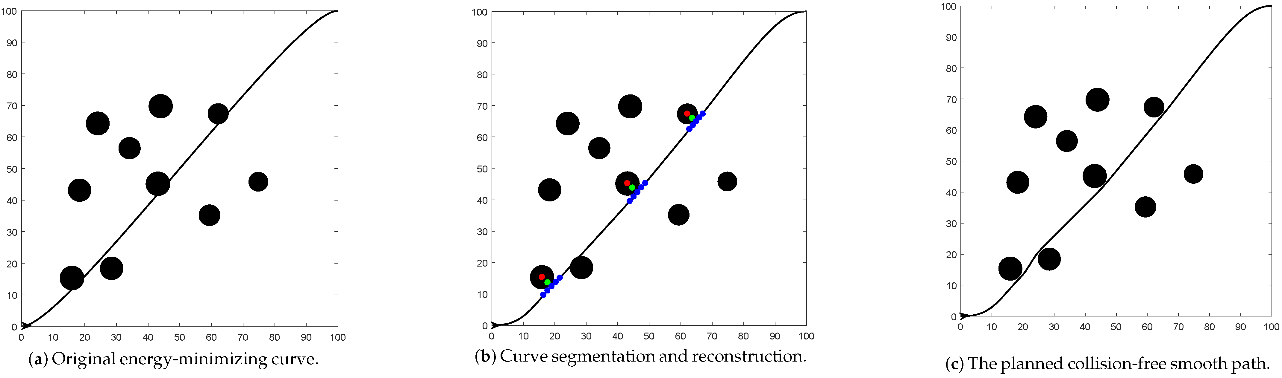
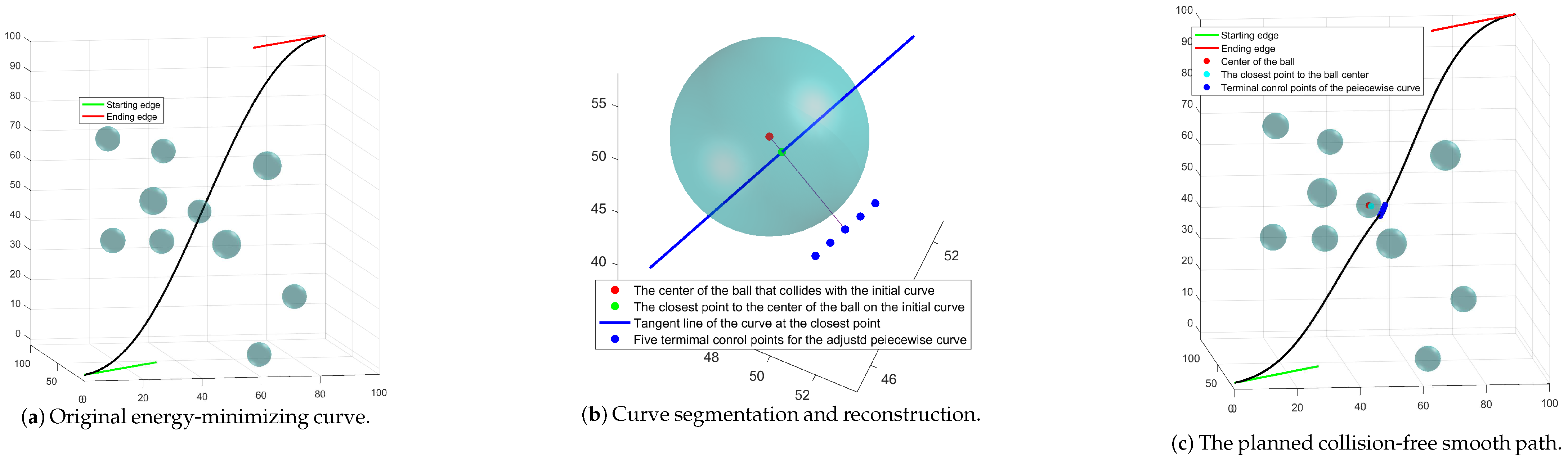
6. Obstacle Avoidance for UAVs Based on Piecewise Curve

6.1. Construction of Smooth Piecewise Path Curve Using Multiple Bézier Curves

In actual path planning scenarios, motion planning implementations leverage algorithmic frameworks to generate a series of discrete pose points, and thereby, multiple short smooth paths can be obtained by using a smooth UAV path planning method. In addition, for a given set of pose vector ${\mathbf{F}}_s(x_s,y_s,z_s,{\varphi }_s,{\psi }_s)$ and ${\mathbf{F}}_f(x_f,y_f,z_f,{\varphi }_f,{\psi }_f)$, sometimes smooth piecewise curve need to be used for obstacle avoidance. For a global smooth path to be achieved, these individual smooth curves must be seamlessly spliced. If these curves are directly connected at the starting and ending points, though the resulting piecewise path is continuous in position, its curvature is discontinuous. In this case, the piecewise path does not meet the flight requirements of UAVs. To address this issue, the pose vectors, namely, the terminal control points of some curve segment, need to be modified.

Suppose the ith smooth UAV path is an n-degree Bézier curve $\mathbf{P}\left(t\right)$ whose control points ${\left\{{\mathbf{p}}_i\right\}}_{i=0}^{i=n}$ are fixed. The end-points properties of the Bézier curve indicate that $\mathbf{P}\left(t\right)$ satisfies

$$\begin{array}{cc}\hfill \mathbf{P}\left(0\right)={\mathbf{p}}_0,& \mathbf{P}\left(1\right)={\mathbf{p}}_n;\hfill \\ \hfill \mathbf{P}\prime \left(0\right)=n({\mathbf{p}}_1-{\mathbf{p}}_0),& \mathbf{P}\prime \left(1\right)=n({\mathbf{p}}_n-{\mathbf{p}}_{n-1});\hfill \\ \hfill \mathbf{P}″\left(0\right)=n(n-1)({\mathbf{p}}_2-2{\mathbf{p}}_1+{\mathbf{p}}_0),& {\mathbf{P}}^{″}\left(1\right)=n(n-1)({\mathbf{p}}_n-2{\mathbf{p}}_{n-1}+{\mathbf{p}}_{n-2}).\hfill \end{array}$$

(10)

Suppose the $(i+1)$th smooth UAV path is a Bézier curve $\mathbf{Q}\left(t\right)$ of degree n whose control points are denoted as ${\left\{{\mathbf{q}}_i\right\}}_{i=0}^{i=n}$. $C^2$ continuity between the two paths means that $\mathbf{P}\left(t\right)$ and $\mathbf{Q}\left(t\right)$ need to satisfy

$$\begin{array}{cc}\hfill & \mathbf{P}\left(1\right)=\mathbf{Q}\left(0\right);\hfill \\ \hfill & \mathbf{P}\prime \left(1\right)=\mathbf{Q}\prime \left(0\right);\hfill \\ \hfill & \mathbf{P}″\left(1\right)=\mathbf{Q}″\left(0\right).\hfill \end{array}$$

Thus, according to the end-points properties of the Bézier curve in Equation (10), to achieve $C^2$ continuity, the terminal control points ${\mathbf{q}}_0,{\mathbf{q}}_1,{\mathbf{q}}_2$ of $\mathbf{Q}\left(t\right)$ should satisfy

$$\begin{array}{cc}\hfill {\mathbf{q}}_0& ={\mathbf{p}}_n;\hfill \\ \hfill {\mathbf{q}}_1& =2{\mathbf{p}}_n-{\mathbf{p}}_{n-1};\hfill \\ \hfill {\mathbf{q}}_2& =4{\mathbf{p}}_n-4{\mathbf{p}}_{n-1}+{\mathbf{p}}_{n-2}.\hfill \end{array}$$

(11)

For the $(i+1)$th path $\mathbf{Q}\left(t\right)$, its initial control points ${\mathbf{q}}_0,{\mathbf{q}}_1,{\mathbf{q}}_2$ are determined by the ith path, and its terminal control points ${\mathbf{q}}_{n-1},{\mathbf{q}}_n$ are obtained by pose information, while the other control points of $\mathbf{Q}\left(t\right)$ are movable. In this case, the smoothness and arc length of $\mathbf{Q}\left(t\right)$ can be optimized by energy minimization by Equation (6).

Example 8. 

The design of a smooth piecewise UAV path by using multiple energy-minimizing Bézier curves is shown in Figure 9. The piecewise UAV path is composed of two 8-degree Bézier curves whose control points are denoted as ${\left\{{\mathbf{p}}_i\right\}}_{i=0}^8$, ${\left\{{\mathbf{q}}_i\right\}}_{i=0}^8$. Here, the positions of the terminal control points ${\mathbf{p}}_0$, ${\mathbf{p}}_1$, and ${\mathbf{p}}_2$ as well as ${\mathbf{p}}_6$, ${\mathbf{p}}_7$, and ${\mathbf{p}}_8$ of the first curve $\left\{\mathbf{P}\right(t)$ are supposed to be fixed. To ensure the position continuity, tangential continuity, and curvature continuity at the junction of the two curves, the position of the control points ${\mathbf{q}}_0$, ${\mathbf{q}}_1$, and ${\mathbf{q}}_2$ of the second curve $\left\{\mathbf{Q}\right(t)$ are determined by ${\mathbf{p}}_6$, ${\mathbf{p}}_7$, and ${\mathbf{p}}_8$ by Equation (11). In addition, the position of the control points ${\mathbf{q}}_8$, ${\mathbf{q}}_7$, and ${\mathbf{q}}_6$ are fixed according to pose constraints. Then, the control points whose positions are unknown are ${\left\{{\mathbf{p}}_i\right\}}_{i=3}^5,{\left\{{\mathbf{q}}_i\right\}}_{i=3}^5$. By minimizing the composite energy functional $E_{comp}\left[\mathbf{P}\right]$ (4), the position of the six movable control points, that is, two energy-minimizing Bézier curves, can be determined.

6.2. Design of Collision-Free Smooth Path for UAVs

For a given set of pose vector ${\mathbf{F}}_s(x_s,y_s,z_s,{\varphi }_s,{\psi }_s)$ and ${\mathbf{F}}_f(x_f,y_f,z_f,{\varphi }_f,{\psi }_f)$ at the starting and the target point, if the resulting energy-minimizing curve passes through some obstacles, the initial energy-minimizing curve need to be segmented at the locations where it collides with an obstacle. Here, an example is given in Figure 10 to illustrates the design of a collision-free smooth path by using multiple energy-minimizing Bézier curves, where the obstacles are represented as the black bullets. As shown in Figure 10a, the initial energy-minimizing Bézier curve pass through an obstacle. In Figure 10b, the red point is the center of the obstacle, denoted as $(x_r,y_r)$, and the radius of the obstacle is represented as r. The green point is the closest point on the initial energy-minimizing curve to the center of the obstacle, which is denoted as $(x_1,y_1)$. In order to avoid the obstacle and achieve $C^2$ continuity, the initial energy-minimizing curve should be divided into two parts. Specifically, the end point ${\mathbf{p}}_n$ of the first segment of the piecewise curve, that is, the starting point ${\overline{\mathbf{p}}}_0$ of the second segment of the piecewise curve, is determined based on the vector $(x_1-x_r,y_1-y_r)$ with $\parallel {\mathbf{p}}_n-(x_r,y_r)\parallel =r+\epsilon$, where $\epsilon >0$; moreover, to avoid the obstacle, the tangent of the piecewise curve at ${\mathbf{p}}_n$ should be perpendicular to the vector $(x_1-x_r,y_1-y_r)$, and thus, the control points ${\mathbf{p}}_{n-2},{\mathbf{p}}_{n-1}$ and ${\overline{\mathbf{p}}}_1,{\overline{\mathbf{p}}}_2$ can be determined with $\parallel {\overline{\mathbf{p}}}_2-{\mathbf{p}}_{n-2}\parallel =2r$ and $({\mathbf{p}}_{n-1}-{\mathbf{p}}_{n-2})=({\mathbf{p}}_n-{\mathbf{p}}_{n-1})=({\overline{\mathbf{p}}}_1-{\overline{\mathbf{p}}}_0)=({\overline{\mathbf{p}}}_2-{\overline{\mathbf{p}}}_1)$ to achieve $C^2$ continuity. As shown in Figure 10b, with minor modification to the initial curve, the constructed piecewise curve effectively avoids the obstacle.

The design of a collision-free smooth path by using multiple energy-minimizing Bézier curves in the scene with another set of obstacles is shown in Figure 11. Analogously, the construction of a collision-free smooth path by using multiple energy-minimizing Bézier curves in 3D space can be achieved.

For 3D scenes, a similar method can be applied for obstacle avoidance. As shown in Figure 12, the blue balls represet the obstacles and the initial planned path intersects with one of the obstacles. To avoid the obstacle, the tangent of the piecewise curve at ${\mathbf{p}}_n$ should be parallel to the tangent line $\mathbf{C}\prime \left(t_{cloest}\right)$ of the curve at the closest point to the center of the ball $(x_r,y_r,z_r)$.

In Figure 13, an example of UAV path planning in a complex environment is presented. In this study, the RRT* algorithm [34] was used for the initial path planning. In the figure, the blue straight line segments indicate the growth process of the random search tree, and the green polyline represents the generated initial path. Then, the proposed method was employed for path smoothing, and the generated smooth curve is represented as the red curve in the figure.

In Figure 14, an example is presented to compare the smoothing effects of 7-degree Bézier curves and 8-degree Bézier curves in path smoothing. The discrete initial path in green was obtained by the RRT* algorithm [34], and the red curve in Figure 14a,b represents the smoothed path obtained using the proposed method with 7-degree Bézier curves and 8-degree Bézier curves, respectively. From Figure 14 (especially the paths within the rectangular boxes), it can be seen that using the 8-degree Bézier curves resulted in a better smoothing effect due to its higher degree of freedom. Here, the calculation time for path smoothing using 7-degree Bézier curves and 8-degree Bézier curves was 1.53 s and 1.77 s, respectively.

7. Results Discussion

(1)

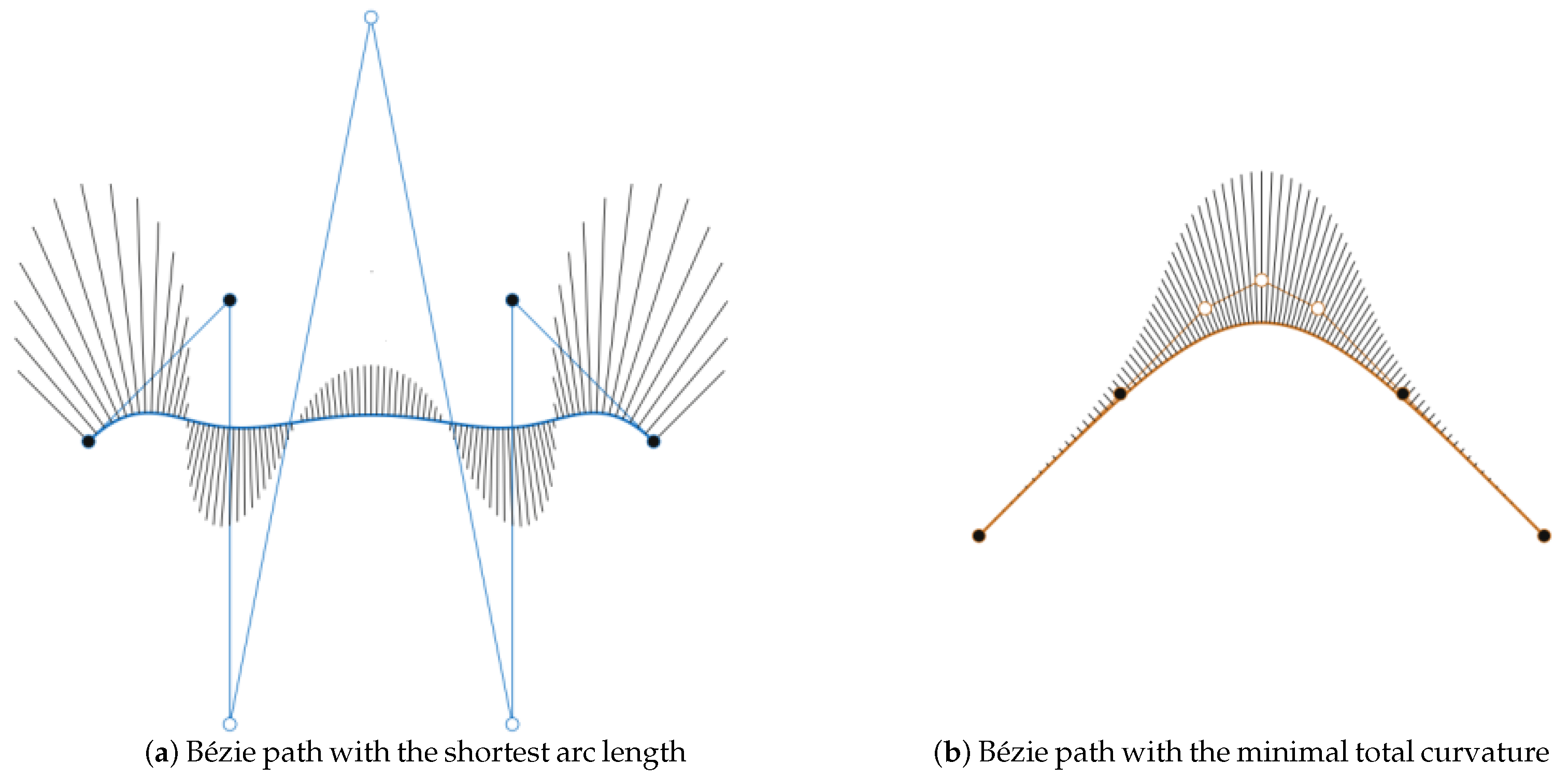
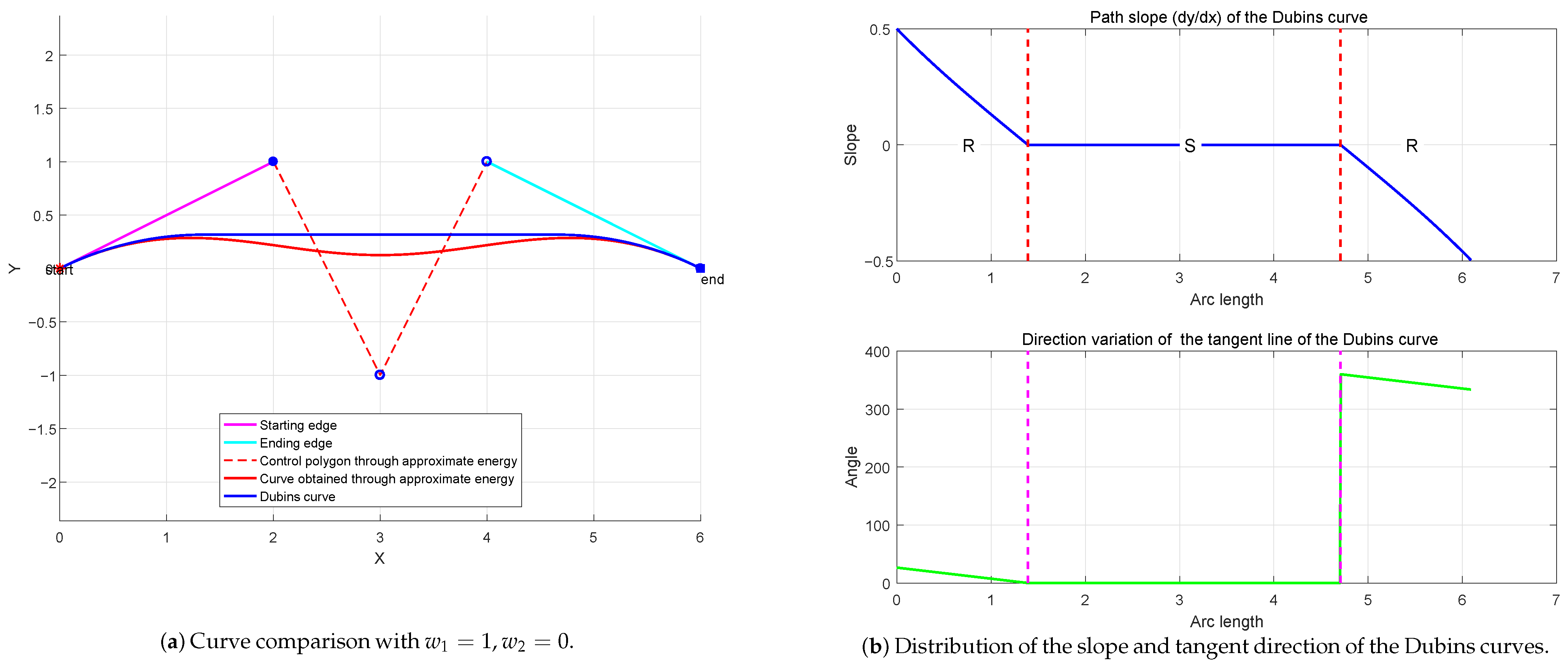
It can be seen from Figure 2a, Figure 3a, Figure 4a and Figure 9a that though the curve optimization based on stretching energy can help obtain UAVs flight path with a very short distance so as to reduce energy consumption and execution time of UAVs, the smoothness of these curves is very poor. Specifically, the overall curvature of these curves is large, especially at the corners of both ends of the curve, which is not conducive to UAV flight.

(2)

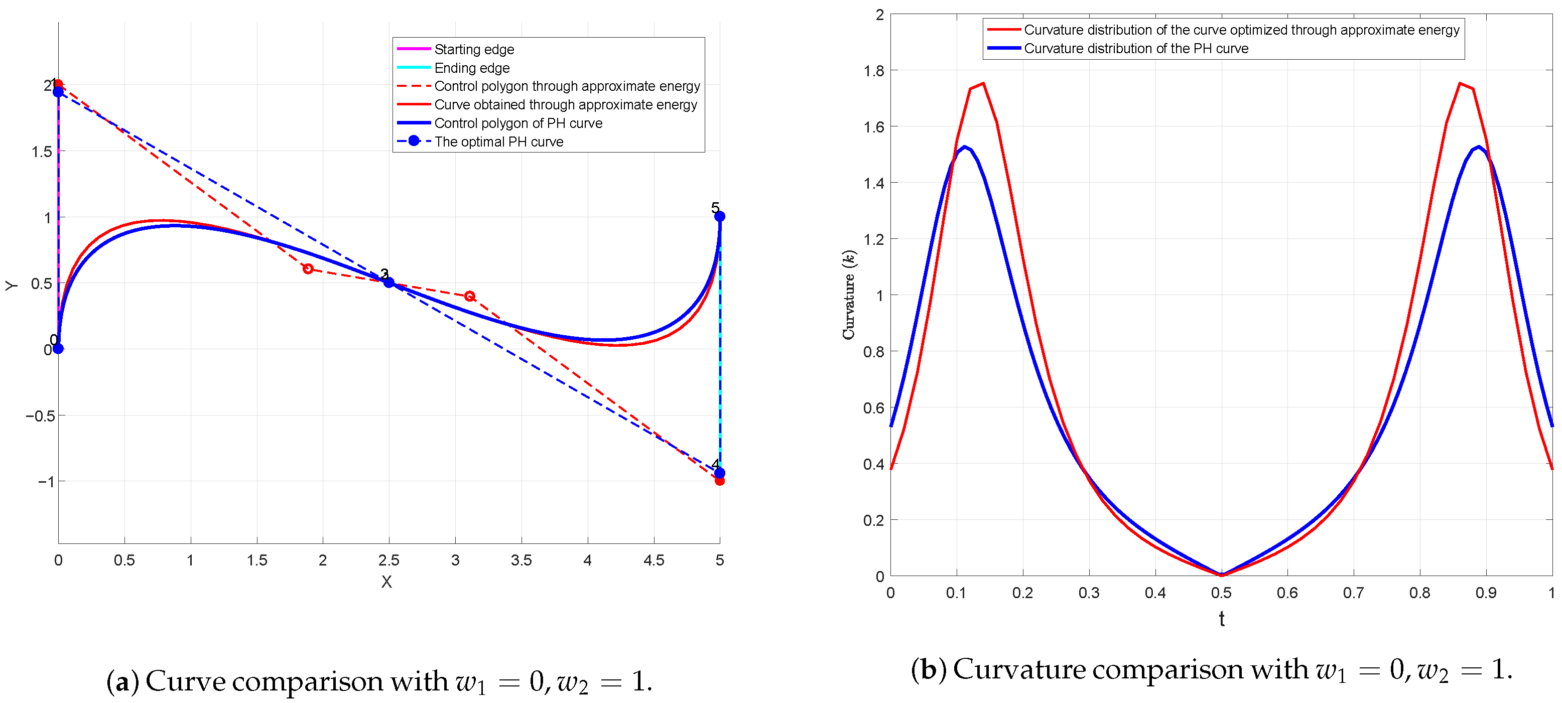
From Figure 2b, Figure 3b, Figure 4b and Figure 9b, it is evident that curve optimization based on bending energy can help obtain a UAV’s flight path with very good smoothness; however, the length of the flight path is usually long, which will increase the energy consumption and execution time of the UAVs. In addition, curve optimization based on bending energy can minimize the overall curvature (integral of curvature) of the curve, but the maximum curvature value of the curve is not necessarily the minimum in the candidate flight curve of UAVs. In UAV path planning, maintaining an instantaneous curvature below aircraft-specific thresholds proves more critical than minimizing total curvature accumulation.

(3)

By contrast, visual analysis of Figure 2c, Figure 3c, Figure 4c and Figure 9c and Figure 2d, Figure 3d, Figure 4d and Figure 9d,e indicates that, on the one hand, optimization based on composite energy can reduce the arc length of path; on the other hand, as can be seen from Figure 3d, Figure 9d and Figure 9e, sometimes the maximum curvature of the curve obtained by optimizing the composite energy is actually smaller than that obtained by optimizing the bending energy only and thus is more conducive to the safe and stable flight of UAVs.

(4)

From Figure 2e, Figure 3e, Figure 4e and Figure 2f, Figure 3f, Figure 4f, it is evident that when $w_1\to 0$ and $w_2\to 1$, namely, $w_1/w_2\to 0$, the shape of the optimal curve is not sensitive to the value changes of the weight parameters $w_1$ and $w_2$. As $w_1$ gradually increases and $w_2$ gradually decreases, namely, as $w_1/w_2$ gradually decreases, the shape of the curve becomes increasingly sensitive to the changes in the values of the weight parameters $w_1$ and $w_2$.

(5)

Visual analysis of Figure 10, Figure 11 and Figure 12 indicates that, by using a $C^2$ continuous piecewise energy-minimizing Bézier curve, a collision-free smooth path with a short length and good smoothness can be obtained.

(6)

Limitations of the proposed method: The study in this paper only considers the direction and curvature constraints of UAVs at the ends of a short path, and other dynamic constraints of UAVs were not fully taken into account. In addition, the study in this paper merely remains at the theoretical analysis level to provides a new theoretical approach; thus, the effectiveness of the method and the optimal values of the weight parameters have not yet been verified on UAVs. Therefore, further improvements are needed in the future.

8. Conclusions

In this paper, a method for the variational design of a smooth UAV path is proposed by using energy-minimizing Bézier curves. In smooth UAV path planning, a composite energy functional is defined by combining the approximate stretching energy and bending energy of curves to balance the arc length and smoothness of the path, and path generation via composite energy minimization can be reduced to solve well-conditioned linear equations. Benchmark tests across various obstacle configurations validate the method’s reliability in producing dynamically feasible paths with good smoothness and short lengths, which can help to improve the safety and stability of UAVs in flight and decrease the energy consumption and execution time of UAVs. Compared to other path planning methods based on Bézier/B-spline curves, the optimal path can be obtained by solving a system of linear equations with less computation cost and time cost using the proposed method instead of step-by-step iterations, which can improve the efficiency of path planning and thus improve the reaction speed and obstacle avoidance ability of UAVs and enable real-time computation for autonomous systems. Applying this method to practical path planning, improving and optimizing the method continuously in practice will be the promising and represents an important direction for future work.

References

1. Abdel-Basset, M.; Mohamed, R.; Alrashdi, I.; Sallam, K.M.; Hameed, I.A. Evolution-based energy-efficient data collection system for UAV-supported IoT: Differential evolution with population size optimization mechanism. Expert Syst. Appl. 2024, 245, 123082. [Google Scholar] [CrossRef]
2. Dayarian, I.; Savelsbergh, M.; Clarke, J. Same-day delivery with drone resupply. Transp. Sci. 2020, 54, 229–249. [Google Scholar] [CrossRef]
3. Liu, Y. An elliptical cover problem in drone delivery network design and its solution algorithms. Eur. J. Oper. Res. 2023, 304, 912–925. [Google Scholar] [CrossRef]
4. Dukkanci, O.; Campbell, J.F.; Kara, B.Y. Facility location decisions for drone delivery: A literature review. Eur. J. Oper. Res. 2023, 316, 397–418. [Google Scholar] [CrossRef]
5. Hu, D.; Ba, Y.; Cao, W.; Lin, C.; Wang, Z. An improved A-Star algorithm for path planning of outdoor distribution robots. ACM Int. Conf. Proc. Ser. 2022, 66, 1–6. [Google Scholar]
6. Long, T. Improved A-star algorithm in efficiency enhancing and path smoothing. In Proceedings of the 2023 IEEE International Conference on Control, Electronics and Computer Technology, ICCECT, Jilin, China, 28–30 April 2023; pp. 28–31. [Google Scholar]
7. Sarbini, R.N.; Ahmad, I.; Bura, R.O.; Simbolon, L. Development of pathfinding using A-star and D-star lite algorithms in video game. J. Theor. Appl. Inf. Technol. 2024, 102, 832–841. [Google Scholar]
8. Liu, Y.; Chen, C.; Wang, Y.; Zhang, T.; Gong, Y. A fast formation obstacle avoidance algorithm for clustered UAVs based on artificial potential field. Aerosp. Sci. Technol. 2024, 147, 108974. [Google Scholar] [CrossRef]
9. Tang, X.; Jia, C.; Liu, Y. Fuzzy enhanced artificial potential field-based mobile car path planning. ACM Int. Conf. Proc. Ser. 2022, 83, 1–6. [Google Scholar]
10. Naderi, K.; Rajamäki, J.; Hämäläinen, P. RT-RRT*: A real-time path planning algorithm based on RRT. In Proceedings of the ACM SIGGRAPH Conference on Motion in Games, Paris, France, 16–18 November 2015; pp. 113–118. [Google Scholar]
11. Armstrong, D.; Jonasson, A. AM-RRT*: Informed sampling-based planning with assisting metric. In Proceedings of the IEEE International Conference on Robotics and Automation, Xi’an, China, 30 May–5 June 2021; pp. 10093–10099. [Google Scholar]
12. Wang, J.; Chi, W.; Li, C.; Meng, M. Efficient robot motion planning using bidirectional-unidirectional RRT extend function. IEEE Trans. Autom. Sci. Eng. 2022, 19, 1859–1868. [Google Scholar] [CrossRef]
13. Ma, H.; Meng, F.; Ye, C.; Wang, J.; Meng, M. Bi-risk-RRT based efficient motion planning for mobile robots. IEEE Trans. Intell. Veh. 2022, 7, 722–733. [Google Scholar] [CrossRef]
14. Zhang, Y.; Wang, H.; Yin, M.; Wang, J.; Hua, C. Bi-AM-RRT*: A Fast and Efficient Sampling-Based Motion Planning Algorithm in Dynamic Environments. IEEE Trans. Intell. Veh. 2023, 9, 1282–1293. [Google Scholar] [CrossRef]
15. Karaman, S.; Frazzoli, E. Incremental sampling-based algorithms for optimal motion planning. Robot. Sci. Syst. 2010, 104, 267–274. [Google Scholar]
16. Islam, F.; Nasir, J.; Malik, U.; Ayaz, Y.; Hasan, O. RRT*-smart: Rapid convergence implementation of RRT* towards optimal solution. In Proceedings of the IEEE International Conference on Mechatronics and Automation, Chengdu, China, 5–8 August 2012; pp. 1651–1656. [Google Scholar]
17. Yi, D.; Thakker, R.; Gulino, C.; Salzman, O.; Srinivasa, S. Generalizing Informed Sampling for Asymptotically-Optimal Sampling-Based Kinodynamic Planning via Markov Chain Monte Carlo. In Proceedings of the 2018 IEEE International Conference on Robotics and Automation (ICRA), Brisbane, QLD, Australia, 21–25 May 2018; pp. 7063–7070. [Google Scholar] [CrossRef]
18. Chen, L.; Shan, Y.; Tian, W.; Li, B.; Cao, D. A fast and efficient double-tree RRT*-like sampling-based planner applying on mobile robotic systems. IEEE/ASME Trans. Mechatron. 2018, 23, 2568–2578. [Google Scholar] [CrossRef]
19. Zhang, Y.; Wang, P.; Cui, K.; Zhou, H.; Yang, J.; Kong, X. An obstacle avoidance path planning and evaluation method for intelligent vehicles based on the B-spline algorithm. Sensors 2023, 23, 8151. [Google Scholar] [CrossRef] [PubMed]
20. Wang, S.; Wu, N.; Huang, J.; Wang, J. Smoothing algorithm of air target track based on improved cubic B-spline curve proceedings of SPIE. Int. Soc. Opt. Eng. 2023, 12756, 127564B. [Google Scholar]
21. Park, S. Three-dimensional dubins-path-guided continuous curvature path smoothing. Appl. Sci. 2022, 12, 11336. [Google Scholar] [CrossRef]
22. Wu, W.; Xu, J.; Gong, C.; Cui, N. Adaptive path following control for miniature unmanned aerial vehicle confined to three-dimensional Dubins path: From take-off to landing. ISA Trans. 2023, 143, 156–167. [Google Scholar] [CrossRef] [PubMed]
23. Ren, H.; Fujisawa, K. Obstacle avoidable G2-continuous trajectory generated with clothoid Spline solution. In Proceedings of the 2021 6th International Conference on Control and Robotics Engineering, ICCRE, Beijing, China, 16–18 April 2021; pp. 23–27. [Google Scholar]
24. Zheng, A.; Li, B.; Zheng, M.; Zhang, L. UAV trajectory planning based on PH curve improved by particle swarm optimization and quasi-newton method. Adv. Intell. Technol. Ind. 2022, 285, 423–433. [Google Scholar]
25. Shao, Z.; Zhou, Z.; Qu, G.; Zhu, X. Reference path planning for UAVs formation flight based on PH curve. Lect. Notes Electr. Eng. 2023, 913, 155–168. [Google Scholar]
26. Celestini, D.; Primatesta, S.; Capello, E. Trajectory Planning for UAVs Based on Interfered Fluid Dynamical System and Bézier Curves. IEEE Robot. Autom. Lett. 2022, 7, 9620–9626. [Google Scholar] [CrossRef]
27. Bulut, V. Path planning of mobile robots in dynamic environment based on analytic geometry and cubic Bézier curve with three shape parameters. Expert Syst. Appl. 2023, 233, 120942. [Google Scholar] [CrossRef]
28. Niu, T.; Wang, L.; Xu, Y.; Wang, J.; Wang, S. Quintic Bézier curve and numerical optimal solution based path planning approach in seismic exploration. Control Eng. Pract. 2024, 145, 105855. [Google Scholar] [CrossRef]
29. Juhász, I.; Róth, Á. Adjusting the Energies of Curves Defined by Control Points. Comput.-Aided Des. 2019, 107, 77–88. [Google Scholar] [CrossRef]
30. Cao, H.; Zheng, H.; Hu, G. Adjusting the energy of Ball surfaces by modifying unfixed control balls. Numer. Algorithms 2022, 89, 749–768. [Google Scholar] [CrossRef]
31. Cao, H.; Zheng, H.; Hu, G. Adjusting the energy of Ball curves by modifying movable control balls. Comput. Appl. Math. 2021, 40, 76. [Google Scholar] [CrossRef]
32. Farin, G. Curves and Surfaces for CAGD: A Practical Guide; Elsevier: Amsterdam, The Netherlands, 2001. [Google Scholar]
33. Prautzsch, H.; Boehm, W.; Paluszny, M. Bézier and B-Spline Techniques; Springer Science & Business Media: Berlin/Heidelberg, Germany, 2002. [Google Scholar]
34. LaValle, L.J.K.; Kuffner, J.J. RRT-Connect: An Efficient Approach to Single-Query Path Planning. IEEE Int. Conf. Robot. Autom. (ICRA) 2000, 2, 473–479. [Google Scholar]
Figure 1. Smooth path planning in 2D space by using a 6-degree Bézier curve.
Mathematics 13 02318 g001
Figure 2. Smooth UAV path planning in 2D space by using a 6-degree Bézier curve.
Mathematics 13 02318 g002
Figure 3. Smooth UAV path planning in 2D space by using another 6-degree Bézier curve.
Mathematics 13 02318 g003aMathematics 13 02318 g003b
Figure 4. Smooth UAV path planning in 3D space by using a 7-degree Bézier curve.
Mathematics 13 02318 g004
Figure 5. Comparison between the curves optimized through approximate energy and accurate bending energy respectively.
Mathematics 13 02318 g005
Figure 6. Comparison between the curves optimized through approximate energy and accurate arc length formula respectively.
Mathematics 13 02318 g006
Figure 7. Comparison between the Dubins curve and the curve optimized through approximate energy.
Mathematics 13 02318 g007
Figure 8. Comparison between PH curve and the curve optimized through approximate energy.
Mathematics 13 02318 g008
Figure 9. Planning of smooth piecewise path by using multiple energy-minimizing Bézier curves.
Mathematics 13 02318 g009
Figure 10. Planning of collision-free smooth path by using multiple energy-minimizing Bézier curves.
Mathematics 13 02318 g010
Figure 11. Planning of collision-free smooth path by using multiple energy-minimizing Bézier curves in the scene with another set of obstacles.
Mathematics 13 02318 g011
Figure 12. Planning of collision-free smooth path by using multiple energy-minimizing Bézier curves in the scene in 3D scene.
Mathematics 13 02318 g012
Figure 13. UAV path planning in complex environments using RRT* combined with the proposed method.
Mathematics 13 02318 g013
Figure 14. Comparison of the smoothing effects of 7-degree and 8-degree Bézier curves in path smoothing.
Mathematics 13 02318 g014