Stability of Stochastic Delayed Recurrent Neural Networks

Abstract

This paper addresses the stability of stochastic delayed recurrent neural networks (SDRNNs), identifying challenges in existing scalar methods, which suffer from strong assumptions and limited applicability. Three key innovations are introduced: (1) weakening noise perturbation conditions by extending diagonal matrix assumptions to non-negative definite matrices; (2) establishing criteria for both mean-square exponential stability and almost sure exponential stability in the absence of input; (3) directly handling complex structures like time-varying delays through matrix analysis. Compared with prior studies, this approach yields broader stability conclusions under weaker conditions, with numerical simulations validating the theoretical effectiveness.

1. Introduction

The concept of stochastic delayed recurrent neural networks (SDRNNs) emerged as a natural extension of traditional recurrent neural networks (RNNs), incorporating stochastic processes and time delays to model more complex and realistic dynamical systems [1,2,3,4,5]. The utility of SDRNNs extends across a broad spectrum of disciplines.For instance, SDRNNs have achieved outstanding results in pattern recognition domains, including speech recognition, handwriting analysis and image classification. Moreover, their inherent stochastic characteristics enable them to effectively adapt and generalize under noisy and uncertain conditions. In addition, SDRNNs are adapted to handling the intricacies of time series data with complex temporal relationships. As a result, they have become indispensable for critical applications like stock market trend prediction, weather forecasting and advanced financial market analysis [6,7,8].

The stability of a dynamical system refers to the network’s ability to reach a steady state or to converge to a bounded trajectory over time, despite the presence of disturbances or initial conditions. In the context of SDRNNs, which include both stochastic processes and time delays, stability is particularly important. For instance, stable SDRNNs exhibit robustness to noise, enabling them to handle the inherent randomness of real-world data and maintain consistent performance.

Conventional stability involves the network’s states progressively nearing an equilibrium point as time approaches infinity, encompassing types such as asymptotic stability [9,10,11,12], exponential stability [13,14,15,16,17,18,19,20,21,22,23] and the probabilistic variant of almost sure exponential stability [24,25]. On the other hand, there also exist alternative stability definitions, such as input-to-state stability. Input-to-state stability focuses on the network’s ability to respond to inputs while preserving boundedness in the face of external disturbances, as detailed in [26,27,28,29,30,31,32,33,34,35].

However, a critical analysis of the literature reveals significant limitations in conventional stability studies. Most existing works rely on scalar approaches, which impose restrictive assumptions (e.g., positive coefficients and diagonal noise structures) that fail to capture the complexity of coupled dynamics in SDRNNs. For instance, the scalar-based mean-square exponential input-to-state stability analysis in [36] assumes Lipschitz noise perturbations with positive diagonal matrices, severely limiting its applicability to systems with non-diagonal or time-varying noise. Additionally, few studies address the coexistence of multiple stabilities (e.g., mean-square and almost sure exponential stability) in input-free systems, leaving a crucial gap in understanding robust dynamics in complex stochastic environments.

To bridge the gaps in the existing literature (e.g., scalar approaches in [36] requiring diagonal noise matrices and positive coefficients), this study introduces a matrix-theory framework. The main contributions, distinguished from prior works, are as follows:

• Assumption relaxation: The authors of [36] assume Lipschitz noise with positive diagonal matrices, while we generalize to non-negative definite matrices (Assumptions 1 and 2), expanding stability analysis to broader noise structures;
• Multiple stabilities coexistence: Unlike single-stability analyses, we concurrently prove mean-square and almost sure exponential stabilities for input-free systems (Theorems 3–5). As far as we are aware, this has not been reported in other studies.
• Complex dynamics handling: Scalar methods struggle with time-varying delays, but our matrix approach directly addresses such structures without equivalent scalar representation.

The structure of this paper is outlined as follows: Section 2 begins with the introduction of essential definitions and preliminaries concerning stochastic delayed recurrent neural networks, placing particular emphasis on the significance of stability analysis. It also addresses the constraints of scalar methods and underscores the requirement for a matrix-based strategy. In Section 3, the primary theorems of the paper are presented. Section 4 offers two numerical examples, thereby illustrating the effectiveness of the obtained results. Section 5 provides a detailed exposition of the proof procedures for the aforementioned theorems. Ultimately, Section 6 serves as the conclusion of the paper, where we summarize our contributions.

2. Model Description and Problem Formulation

Zhu et al. considered the mean-square exponential input-to-state stability of SDRNNs in [36]:

$$\left\{\begin{array}{cc}\hfill d{X}_i\left(t\right)=& \left[-d_i{X}_i\left(t\right)+\sum _{m=1}^n{a}_{im}{f}_m\left(X_m\left(t\right)\right)+\sum _{m=1}^n{b}_{im}{g}_m\left(X_m(t-\overline{\tau })\right)\right.\hfill \\ \hfill & \left.+\sum _{m=1}^n{c}_{im}{h}_m\left(X_m(t-\tau \left(t\right))\right)+u_i\left(t\right)\right]dt\hfill \\ \hfill & +\sum _{m=1}^n{\sigma }_{im}\left(X_m\left(t\right),X_m(t-\overline{\tau }),X_m(t-\tau \left(t\right))\right)d{W}_m\left(t\right),\hfill \\ \hfill X_i\left(t\right)=& {\mathrm{\Psi }}_i\left(t\right),-\overline{\tau }\le t\le 0\hfill \end{array}\right.$$

(1)

for any $t\ge 0$ with i ranging from 1 to n.

Firstly, an explanation of the functions appearing in Itô-type Equation (1) is provided. $X_k\left(t\right)$ denotes the state variable of the $k^{th}$ neuron at a given time t. Moreover, $f_m\left(x_m(·)\right)$, $g_m\left(x_m(·)\right)$ and $h_m\left(x_m(·)\right)$ represent the activation functions of the $m^{th}$ neuron at the same time instance. Additionally, the function $u_k(·)$ signifies the regulatory input for the $k^{th}$ neuron at that moment, and $\mathit{u}=(u_1\left(t\right),u_2\left(t\right),\dots ,u_n\left(t\right))$ belongs to $L^{\infty }([0,\infty );{\mathbb{R}}^n)$, where $L^{\infty }$ denotes the space of essentially bounded measurable functions satisfying ${\parallel \mathit{u}\parallel }_{\infty }=\underset{t\ge 0}{ess\; sup}\left|\mathit{u}\left(t\right)\right|<\infty$.

Furthermore, the stochastic term ${\sigma }_{im}$, which is a function from ${\mathbb{R}}^3$ to $\mathbb{R}$, is Borel-measurable. Let $(\mathrm{\Omega },\mathcal{F},{\left\{{\mathcal{F}}_t\right\}}_{t\ge 0},\mathbb{P})$ be a complete probability space where the filtration ${\left\{{\mathcal{F}}_t\right\}}_{t\ge 0}$ is non-decreasing, ${\mathcal{F}}_t$ contains all $\mathbb{P}$-null sets and is naturally generated by the underlying Wiener processes $W_j={\left(W_j\left(t\right)\right)}_{t\ge 0}$, see [37]. Note that both constant and time-varying delays are considered simultaneously. The constant delay $\overline{\tau }$ typically corresponds to the fixed physical transmission delay in the system, while the time-varying delay $\tau \left(t\right)$ is used to describe the delay factors that fluctuate over time in the system. We assume that $\tau \left(t\right)$ is differentiable and fulfills $0\le \tau \left(t\right)\le \overline{\tau }$ and $\dot{\tau }\left(t\right)\le \rho <1$, with $\overline{\tau }$ and $\rho$ being positive constants.

Next, we provide an explanation for the parameters within Equation (1). The coefficient $d_k$ signifies the intensity of the self-feedback link for the $k^{th}$ unit. The coefficients $a_{lm}$, $b_{lm}$ and $c_{lm}$ denote the influence strengths of the $m^{th}$ unit on the $l^{th}$ unit at the moment t.

Finally, we introduce some notations that will be used throughout this paper. ${\ell }_{\infty }$ is defined as the collection of essentially bounded functions from the interval $[0,\infty )$ into ${\mathbb{R}}^n$, satisfying ${\parallel \mathit{u}\parallel }_{\infty }={esssup}_{t\ge 0}\left|\mathit{u}\left(t\right)\right|<\infty$. We use $C\left([-\overline{\tau },0];{\mathbb{R}}^n\right)$ to denote the set of continuous functions $\psi$ over $[-\overline{\tau },0]$ into ${\mathbb{R}}^n$, equipped with $\parallel \psi \parallel ={sup}_{-\overline{\tau }\le s\le 0}\left|\psi \left(s\right)\right|$. The notation $L_{{\mathcal{F}}_0}^2\left([-\overline{\tau },0];{\mathbb{R}}^n\right)$ refers to the collection of all ${\mathcal{F}}_0$-measurable random variables $\psi$ that take values in $C\left([-\overline{\tau },0];{\mathbb{R}}^n\right)$ and satisfy ${\int }_{-\overline{\tau }}^0\mathbf{E}{\left|\psi \left(y\right)\right|}^{2}dy<\infty$, with $\mathbf{E}[·]$ denoting the expectation operator with respect to the probability measure $\mathbb{P}$.

This paper begins by expressing Equation (1) in a vector format as

$$\left\{\begin{array}{c}\mathrm{d}\mathbf{X}\left(t\right)=[-D\mathbf{X}\left(t\right)+A\mathbf{f}\left(\mathbf{X}\left(t\right)\right)+B\mathbf{g}\left(\mathbf{X}(t-\overline{\tau })\right)+C\mathbf{h}\left(\mathbf{X}(t-\tau \left(t\right))\right)+\mathbf{u}\left(t\right)]dt+\delta \left(\mathbf{X}\left(\mathit{t}\right)\right)\mathrm{d}\mathbf{W}\left(t\right)\hfill \\ \mathbf{X}\left(t\right)=\mathbf{\Psi }\left(t\right)\hfill \end{array}\right.$$

(2)

with

$$\begin{array}{c}\hfill \begin{array}{c}A={\left(a_{im}\right)}_{n,n},B={\left(b_{im}\right)}_{n,n},C={\left(c_{im}\right)}_{n,n},D=\mathrm{d}\mathrm{i}\mathrm{a}\mathrm{g}(d_1,\dots ,d_n),\hfill \\ \mathbf{X}\left(t\right)={(X_1\left(t\right),\dots ,X_n\left(t\right))}^T,\mathbf{f}\left(\mathbf{X}\left(t\right)\right)={(f_1\left(X_1\left(t\right)\right),\dots ,f_n\left(X_n\left(t\right)\right))}^T,\hfill \\ \mathbf{g}\left(\mathbf{X}\left(t\right)\right)={(g_1\left(X_1\left(t\right)\right),\dots ,g_n\left(X_n\left(t\right)\right))}^T,\mathbf{h}\left(\mathbf{X}\left(t\right)\right)={(h_1\left(X_1\left(t\right)\right),\dots ,h_n\left(X_n\left(t\right)\right))}^T,\hfill \\ \mathit{\delta }\left(\mathbf{X}\left(t\right)\right)={\left({\delta }_{im}(X_m\left(t\right),X_m(t-\overline{\tau }),X_m(t-\tau \left(t\right)))\right)}_{n,n},\mathbf{\Psi }\left(t\right)={({\mathrm{\Psi }}_1\left(t\right),\dots ,{\mathrm{\Psi }}_n\left(t\right))}^T.\hfill \end{array}\end{array}$$

Remark 1.

It is important to observe that recasting Equation (1) into the vector format (2) constitutes more than an equivalent formulation. The vector notation facilitates a more relaxed discussion of the general forms of functions $\mathbf{f},\mathbf{g},\mathbf{h}$ and $\mathit{\delta }.$ For instance, we can broaden the condition of $\mathit{f}\left(\mathit{X}\left(t\right)\right)={(f_1\left(X_1\left(t\right)\right),\dots ,f_n\left(X_n\left(t\right)\right))}^T$ to

$$\mathbf{f}(\mathit{X}\left(t\right)={(f_1\left(\mathbf{X}\left(t\right)\right),\dots ,f_n\left(\mathbf{X}\left(t\right)\right))}^T,$$

and the integrity of all subsequent discussions remains unaffected. In such cases, discussing the problem using the component form becomes inconvenient. This relaxation suggests that the scope of our work extends to applications beyond the realm of neural networks.

We will also consider system (2) with $\mathbf{u}\left(t\right)=\mathbf{0}.$ In this case, it simplifies to the following system

$$\left\{\begin{array}{c}\mathrm{d}\mathbf{X}\left(t\right)=[-D\mathbf{X}\left(t\right)+A\mathbf{f}\left(\mathbf{X}\left(t\right)\right)+B\mathbf{g}\left(\mathbf{X}(t-\overline{\tau })\right)+C\mathbf{h}\left(\mathbf{X}(t-\tau \left(t\right))\right)]dt+\delta \left(\mathbf{X}\left(\mathit{t}\right)\right)\mathrm{d}\mathbf{W}\left(t\right)\hfill \\ \mathbf{X}\left(t\right)=\mathbf{\Psi }\left(t\right)\hfill \end{array}\right.$$

(3)

It is crucial to note that Equations (2) and (3) are Itô-type stochastic differential equations, consistent with Equation (1). Below, we present several definitions of stability for the trivial solution of Equations (2) and (3).

Definition 1.

The trivial solution of system (2) is mean-square exponentially input-to-state-stable if, for any $\mathrm{\Psi }\in L_{{\mathcal{F}}_0}^2\left([-\overline{\tau },0];{\mathbb{R}}^n\right)$ and $\mathbf{u}\in L^{\infty }([0,\infty );{\mathbb{R}}^n)$, there exist positive scalars ${\alpha }_1,{\alpha }_2,{\alpha }_3$ such that

$$\mathbf{E}{\left|\mathbf{X}(t;\mathrm{\Psi })\right|}^2\le {\alpha }_1{e}^{-{\alpha }_{2}t}{\mathbf{E}\parallel \mathrm{\Psi }\parallel }^2+{\alpha }_3{\parallel \mathbf{u}\parallel }_{\infty }^2.$$

Definition 2.

The trivial solution of system (3) is mean-square exponentially stable if, for all $\mathrm{\Psi }\in L_{{\mathcal{F}}_0}^2\left([-\overline{\tau },0];{\mathbb{R}}^n\right)$, there exist positive scalars ${\alpha }_1,{\alpha }_2$ such that

$$\mathbf{E}{\left|\mathbf{X}(t;\mathrm{\Psi })\right|}^2\le {\alpha }_1{e}^{-{\alpha }_{2}t}\mathbf{E}{\parallel \mathrm{\Psi }\parallel }^2.$$

Definition 3.

The trivial solution of system (3) is almost surely exponentially stable if, for each $\mathrm{\Psi }\in L_{{\mathcal{F}}_0}^2\left([-\overline{\tau },0];{\mathbb{R}}^n\right)$, there exists a positive scalar γ such that

$$\underset{t\to \infty }{lim\; sup}{\displaystyle \frac{1}{t}}log\left(\left|\mathbf{X}\right(t;\mathrm{\Psi }\left)\right|\right)\le -{\displaystyle \frac{\gamma }{2}}.a.s.$$

Throughout the paper, we adhere to foundational assumptions as follows.

Assumption 1.

Assume that $\mathbf{f}\left(\mathbf{0}\right)=\mathbf{0},\mathbf{g}\left(\mathbf{0}\right)=\mathbf{0},\mathbf{h}\left(\mathbf{0}\right)=\mathbf{0}$ and there exist positive scalars $L_1,L_2,L_3$ such that for any $z_1,z_2\in R^n$,

$$\begin{array}{c}\hfill |\mathbf{f}\left({\mathbf{z}}_{\mathbf{1}}\right)-\mathbf{f}\left({\mathbf{z}}_{\mathbf{2}}\right)|⩽L_1|{\mathbf{z}}_{\mathbf{1}}-{\mathbf{z}}_{\mathbf{2}}|,|\mathbf{g}\left({\mathbf{z}}_{\mathbf{1}}\right)-\mathbf{g}\left({\mathbf{z}}_{\mathbf{2}}\right)|⩽L_2|{\mathbf{z}}_{\mathbf{1}}-{\mathbf{z}}_{\mathbf{2}}|,|\mathbf{h}\left({\mathbf{z}}_{\mathbf{1}}\right)-\mathbf{h}\left({\mathbf{z}}_{\mathbf{2}}\right)|⩽L_3|{\mathbf{z}}_{\mathbf{1}}-{\mathbf{z}}_{\mathbf{2}}|.\end{array}$$

(4)

Furthermore, we assume that there exist symmetric nonnegative-definite matrices $C_1,C_2,C_3$ such that

$$\begin{array}{c}\hfill tr\left({\delta }^T\left(\mathbf{X}\left(t\right)\right)\delta \left(\mathbf{X}\left(t\right)\right)\right)⩽{\mathbf{X}}^T\left(t\right)C_1\mathbf{X}\left(t\right)+{\mathbf{X}}^T(t-\overline{\tau })C_2\mathbf{X}(t-\overline{\tau })+{\mathbf{X}}^T(t-\tau \left(t\right))C_3(\mathbf{X}(t-\tau \left(t\right))\end{array}$$

(5)

Assumption 2.

Assume that there exist symmetrical matrices $F_i^{\left(j\right)},i=1,2,j=1,2,3$ and symmetrical positive definite matrix P such that $H_1,H_2,H_3$ are non-positive definite with

$$\begin{array}{c}\hfill H_1=\left(\begin{array}{cc}{F}_1^{\left(1\right)}& PA\\ A^T{P}^T& F_2^{\left(1\right)}\end{array}\right),H_2=\left(\begin{array}{cc}{F}_1^{\left(2\right)}& PB\\ B^T{P}^T& F_2^{\left(2\right)}\end{array}\right),H_3=\left(\begin{array}{cc}{F}_1^{\left(3\right)}& PC\\ C^T{P}^T& F_2^{\left(3\right)}\end{array}\right)\end{array}$$

(6)

Remark 2.

It follows from Assumptions 1 that for any $\mathbf{z}\in R^n$,

$$\left|\mathbf{f}\left(\mathbf{z}\right)\right|⩽L_1\left|\mathbf{z}\right|,\left|\mathbf{g}\left(\mathbf{z}\right)\right|⩽L_2\left|\mathbf{z}\right|,\left|\mathbf{h}\left(\mathbf{z}\right)\right|⩽L_3\left|\mathbf{z}\right|.$$

(7)

Remark 3.

In this study, we assume that the matrices $C_1,C_2,C_3$ in Equation (5) are non-negative definite. In comparison, the assumption made in [36] only considers the case where these matrices are diagonal. The reader is referred to [36] for the requirement

$${\left[{\sigma }_{ij}\left(x_1,y_1,z_1\right)-{\sigma }_{ij}\left(x_2,y_2,z_2\right)\right]}^2\le {\mu }_{ij}{\left(x_1-x_2\right)}^2+{\nu }_{ij}{\left(y_1-y_2\right)}^2+{\delta }_{ij}{\left(z_1-z_2\right)}^2$$

for any $x_1,x_2,y_1,y_2,z_1,z_2\in \mathbb{R},i,j=1,2,\dots ,n$, and ${\mu }_{ij},{\nu }_{ij},{\delta }_{ij}$ are defined to be nonnegative constants.

Remark 4.

Similarly, we can also generalize the assumption in Equation (4). Assume that for any $z_1,z_2\in R^n$,

$$\begin{array}{c}\hfill |\mathbf{f}\left({\mathbf{z}}_{\mathbf{1}}\right)-\mathbf{f}\left({\mathbf{z}}_{\mathbf{2}}\right){|}^2⩽{({\mathbf{z}}_{\mathbf{1}}-{\mathbf{z}}_{\mathbf{2}})}^T{L}_1{({\mathbf{z}}_{\mathbf{1}}-{\mathbf{z}}_{\mathbf{2}})}^T,\\ \hfill |\mathbf{g}\left({\mathbf{z}}_{\mathbf{1}}\right)-\mathbf{f}\left({\mathbf{z}}_{\mathbf{2}}\right){|}^2⩽{({\mathbf{z}}_{\mathbf{1}}-{\mathbf{z}}_{\mathbf{2}})}^T{L}_2{({\mathbf{z}}_{\mathbf{1}}-{\mathbf{z}}_{\mathbf{2}})}^T,\\ \hfill |\mathbf{h}\left({\mathbf{z}}_{\mathbf{1}}\right)-\mathbf{f}\left({\mathbf{z}}_{\mathbf{2}}\right){|}^2⩽{({\mathbf{z}}_{\mathbf{1}}-{\mathbf{z}}_{\mathbf{2}})}^T{L}_3{({\mathbf{z}}_{\mathbf{1}}-{\mathbf{z}}_{\mathbf{2}})}^T,\end{array}$$

where $L_1,L_2,L_3$ are non-negative definite matrices. This paper maintains the Assumption (4), and interested readers can follow our approach to derive conclusions under the broader assumption.

Remark 5.

Pertaining to Assumption 2, the following question naturally emerges: given an $n\times n$ matrix A, what criteria should be applied to select symmetric matrices $F_1$ and $F_2$ such that the block matrix

$$\left(\begin{array}{cc}{F}_1& A\\ A^T& F_2\end{array}\right)$$

is non-positive definite? Utilizing Lemma A1 from the Appendix A, we know that in order for the matrices $H_1,H_2,H_3$ in Assumption 2 to be non-positive definite, the corresponding matrices $F_j^i$ must be non-positive definite where $i=1,2,j=1,2,3$.

Remark 6.

Under Assumption 2, let ${\lambda }^{\left(1\right)},{\lambda }^{\left(2\right)},{\lambda }^{\left(3\right)}$ denote the smallest eigenvalues of $F_2^{\left(1\right)},F_2^{\left(2\right)},F_2^{\left(3\right)}$, respectively. Then we derive from Remark 5

$${\lambda }^{\left(1\right)}\le 0,{\lambda }^{\left(2\right)}\le 0,{\lambda }^{\left(3\right)}\le 0.$$

3. Main Results

We begin by presenting the theorem on mean-square exponentially input-to-state stability for Equation (1) as detailed in [36].

Assumption 3

([36]). Assume that

$$\begin{array}{c}\hfill \left|f_k\left(z_1\right)-f_k\left(z_2\right)\right|\le l_k|z_1-z_2|,\left|g_k\left(z_1\right)-g_k\left(z_2\right)\right|\le m_k|z_1-z_2|,\left|h_k\left(z_1\right)-h_k\left(z_2\right)\right|\le n_k|z_1-z_2|,\end{array}$$

for any $z_1,z_2\in \mathbb{R},k=1,2,\dots ,n$, and $l_k,m_k,n_k$ are defined to be positive constants.

Assumption 4

([36]). Assume that

$$\begin{array}{c}\hfill {\left[{\sigma }_{ij}(x_1,y_1,z_1)-{\sigma }_{ij}(x_2,y_2,z_2)\right]}^2\le {\mu }_{ij}{(x_1-x_2)}^2+{\nu }_{ij}{(y_1-y_2)}^2+{\delta }_{ij}{(z_1-z_2)}^2,\end{array}$$

for any $x_1,x_2,y_1,y_2,z_1,z_2\in \mathbb{R},i,j=1,2,\dots ,n$, and ${\mu }_{ij},{\nu }_{ij},{\delta }_{ij}$ are defined to be nonnegative constants.

Assumption 5

([36]). $f_k\left(0\right)=g_k\left(0\right)=h_k\left(0\right)=u_k\left(0\right)=0,{\sigma }_{km}(0,0,0)=0,k,m=$$1,2,\dots ,n$.

Theorem 4

([36]). If Assumptions 3–5 are satisfied, the trivial solution of system (1) is mean-square exponentially input-to-state-stable, provided that there exist positive scalars λ, $p_i$, $q_i$ and $r_i$ for $i=1,2,\dots ,n$ such that

$$\begin{array}{c}\hfill \begin{array}{c}\begin{array}{c}\hfill 2d_i{p}_i\ge (\lambda +1)p_i+q_i+r_i+\sum _{j=1}^n{p}_j{\mu }_{ji}+p_i\sum _{j=1}^n\left|a_{ij}\right|l_j\\ \hfill +\sum _{j=1}^n{p}_j\left|a_{ji}\right|l_i+p_i\sum _{j=1}^n\left|b_{ij}\right|m_j+p_i\sum _{j=1}^n\left|c_{ij}\right|n_j,\end{array}\hfill \\ q_i\ge \sum _{j=1}^n{e}^{\lambda \overline{\tau }}{p}_j\left|b_{ji}\right|m_i+\sum _{j=1}^n{e}^{\lambda \overline{\tau }}{p}_j{\nu }_{ji},\hfill \\ (1-\rho )r_i\ge \sum _{j=1}^n{e}^{\lambda \overline{\tau }}{p}_j\left|c_{ji}\right|n_i+\sum _{j=1}^n{e}^{\lambda \overline{\tau }}{p}_j{\delta }_{ji}.\hfill \end{array}\end{array}$$

Subsequently, we introduce the stability criteria of this paper and compare them with the results of Theorem 4. To establish the next theorems, we define the following matrices

$$\begin{array}{c}\hfill \begin{array}{c}{H}_4=P{P}^T+\lambda P+Q+R+{\lambda }_{max}\left(P\right)C_1-2PD-F_1^{\left(1\right)}-F_1^{\left(2\right)}-F_1^{\left(3\right)}-{\lambda }^{\left(1\right)}{L}_1^{2}I\hfill \\ H_5={\lambda }_{max}\left(P\right)C_2-e^{-\lambda \overline{\tau }}Q-{\lambda }^{\left(2\right)}{L}_2^{2}I,\hfill \\ H_6={\lambda }_{max}\left(P\right)C_3-e^{-\lambda \overline{\tau }}(1-\rho )R-{\lambda }^{\left(3\right)}{L}_3^{2}I.\hfill \end{array}\end{array}$$

(8)

where ${\lambda }^{\left(1\right)},{\lambda }^{\left(2\right)},{\lambda }^{\left(3\right)}$ are presented in Remark 6 and I represents the $n\times n$ identity matrix.

Theorem 5.

If Assumptions 1 and 2 are fulfilled, the trivial solution of system (2) is mean-square exponential input-to-state-stable if there exist positive scalars λ and positive definite matrices $P,Q,R$ such that $H_4,H_5,H_6$ are all non-positive definite.

Remark 7.

Let the matrices $C_1,C_2,C_3$ in Assumption 1 and $P,Q,R$ in Theorem 5 be diagonal matrices, and it can be readily observed that Theorem 5 reduces to Theorem 4. This implies that our theorem encompasses the results of [36].

On the other hand, if $\mathbf{u}\left(t\right)=\mathbf{0}$, Theorem 5 reduces to the mean-square exponential stability of system (3). This reduction is stated as follows.

Theorem 6.

If Assumptions 1 and 2 are satisfied, the trivial solution of system (3) is mean-square exponential-stable if there exist positive scalars λ and positive definite matrices $P,Q,R$ such that $H_4,H_5,H_6$ are all non-positive definite.

Theorem 7.

If Assumptions 1 and 2 are fulfilled, the trivial solution of system (3) is almost surely exponential-stable if there exist positive scalars λ and positive definite matrices $P,Q,R$ such that $H_4+e^{\lambda \overline{\tau }}(H_5+H_6)$ is non-positive definite. To be exact, we have

$$\underset{s\to \infty }{lim\; sup}{\displaystyle \frac{1}{s}}log\left(\right|X(s;\mathrm{\Psi })\left|\right)⩽-{\displaystyle \frac{\lambda }{2}}a.s.$$

(9)

Remark 8.

Theorem 2 and Theorem 3, respectively, provide the conditions for the mean-square exponential stability and almost surely exponential stability for the trivial solutions of Equation (3). It is well known that exponential stability implies the almost surely exponential stability under certain conditions. By comparing our two theorems, this fact is further corroborated.

Below, we present the conditions under which the trivial solution of Equation (3) satisfies both types of stability.

Theorem 8.

If Assumptions 1 and 2 are fulfilled, the trivial solution of system (3) is both mean-square exponential-stable and almost surely exponential-stable if there exist positive scalars λ and positive definite matrices $P,Q,R$ such that $H_4,H_5,H_6$ are non-positive definite.

Remark 9.

In Theorems 6–8, we obtain several stability criteria for system (3). By choosing appropriate Lyapunov–Krasovskii functional and a refined application of stochastic analysis theory, we achieve both mean-square exponential stability and almost sure exponential stability for SDRNNs with no input. As far as we are aware, this has not been reported in other studies.

4. Illustrative Examples

In this section, we will present simulation experiments in two-dimensional and three-dimensional spaces. Numerical solutions were obtained via the Euler–Maruyama scheme with fixed step-size $\Delta t=0.001$. The strong convergence order of 0.5 under global Lipschitz conditions was first proven by Gikhman and Skorochod [38]. We note that more advanced methods exist, such as the stochastic balanced drift-implicit Theta methods [39], which may offer improved stability for stiff systems. Reference [40] provides additional implementation insights for stochastic simulation.

Example 1.

(2-D case) Consider the 2-D SDRNNs (2) with

$$A=\left[\begin{array}{cc}0.0100& -0.1001\\ 0.0400& 0.0300\end{array}\right],B=\left[\begin{array}{cc}0.0020& 0.0030\\ -0.0001& -0.0020\end{array}\right],C=\left[\begin{array}{cc}0.0400& -0.0060\\ 0.0030& 0.2210\end{array}\right],D=\left[\begin{array}{cc}21& 0\\ 0& 17.2\end{array}\right].$$

(1) 

Select the following functions and parameters:

$$\begin{array}{c}\hfill \begin{array}{c}\lambda =0.4,\overline{\tau }=2,\rho =0.4,\tau \left(t\right)=0.4sin\left(t\right)+0.8,L_1=2.1,L_2=1,L_3=3.2,\hfill \\ \mathbf{f}\left(x_1,x_2\right)={\left(2sin\left(x_1\right),2.1sin\left(x_2\right)\right)}^T,\mathbf{g}\left(x_1,x_2\right)={\left(cos\left(x_1\right),0.5x_2\right)}^T,\hfill \\ \mathbf{h}\left(x_1,x_2\right)={\left(3.2x_1,sin\left(x_2\right)\right)}^T,\mathbf{u}\left(t\right)={\left(0.02cos\left(t\right),-0.01sin\left(t\right)\right)}^T,\hfill \\ \delta \left(\mathbf{x}\left(t\right)\right)=\left(\begin{array}{cc}0.03x_1\left(t\right)+0.025x_1(t-\overline{\tau })\hfill & 0.02x_2\left(t\right)+0.023x_2(t-\overline{\tau })\hfill \\ 0.026x_1\left(t\right)+0.033x_1(t-\tau \left(t\right))\hfill & 0.02x_2\left(t\right)+0.1x_2(t-\tau \left(t\right))\hfill \end{array}\right),\hfill \\ C_1=\left[\begin{array}{cc}0.1& 0.1\\ 0.1& 0.2\end{array}\right],C_2=\left[\begin{array}{cc}0.12& 0.24\\ 0.24& 0.1\end{array}\right],C_3=\left[\begin{array}{cc}0.3& 0.15\\ 0.15& 0.3\end{array}\right]\hfill \end{array}\end{array}$$

With these choices, Assumption 1 is satisfied.

(2) 

Define matrices as follows

$$\begin{array}{cc}\hfill & P=\left[\begin{array}{cc}1& 0\\ 0& 1\end{array}\right],Q=\left[\begin{array}{cc}1.3799& 0.5341\\ 0.5341& 3.3384\end{array}\right],R=\left[\begin{array}{cc}12.6198& 0.5564\\ 0.5564& 12.6198\end{array}\right],\hfill \\ \hfill & F_1^{\left(1\right)}=\left[\begin{array}{cc}-1.0000& 0\\ 0& -1.0000\end{array}\right],F_1^{\left(2\right)}=\left[\begin{array}{cc}-1.0100& 0\\ 0& -1.0100\end{array}\right],F_1^{\left(3\right)}=\left[\begin{array}{cc}-1.0100& 0\\ 0& -1.0100\end{array}\right],\hfill \\ \hfill & F_2^{\left(1\right)}=\left[\begin{array}{cc}-0.0017& -0.0002\\ -0.0002& -0.0110\end{array}\right],F_2^{\left(2\right)}=\left[\begin{array}{cc}-0.0005& -0.0008\\ -0.0008& -0.0001\end{array}\right],F_2^{\left(3\right)}=\left[\begin{array}{cc}-0.0068& -0.0018\\ -0.0018& -0.2053\end{array}\right].\hfill \end{array}$$

with ${\lambda }^{\left(1\right)}=-0.0110,{\lambda }^{\left(2\right)}=0,{\lambda }^{\left(3\right)}=-0.2053,$ it can be obtained by Definition (6) that

$$\begin{array}{cc}\hfill & H_1=\left[\begin{array}{cccc}-1& 0& 0.0100& -0.1000\\ 0& -1& 0.0400& 0.0300\\ 0.0100& 0.0400& -0.0017& -0.0002\\ -0.1000& 0.0300& -0.0002& -0.0110\end{array}\right],\hfill \\ \hfill & H_2=\left[\begin{array}{cccc}-1.0100& 0& 0.0020& 0.0030\\ 0& -1.0100& -0.0001& -0.0020\\ 0.0020& -0.0001& -0.0005& -0.0008\\ 0.0030& -0.0020& -0.0008& -0.0001\end{array}\right],\hfill \\ \hfill & H_3=\left[\begin{array}{cccc}-1.0100& 0& 0.0400& -0.0060\\ 0& -1.0100& 0.0030& 0.2210\\ 0.0400& 0.0030& -0.0068& -0.0018\\ -0.0060& 0.2210& -0.0018& -0.2053\end{array}\right].\hfill \end{array}$$

It is straightforward to verify that $H_1,H_2,H_3$ are non-positive definite, which means that Assumption 2 is satisfied.

(3) 

It follows from Definition (8) that

$$H_4=\left[\begin{array}{cc}-23.4318& 1.1905\\ 1.1905& -13.7733\end{array}\right],H_5=\left[\begin{array}{cc}-0.5& 0\\ 0& -0.5\end{array}\right],H_6=\left[\begin{array}{cc}-1& 0\\ 0& -1\end{array}\right].$$

It is straightforward to demonstrate that $H_4,H_5,H_6$ are non-positive definite.

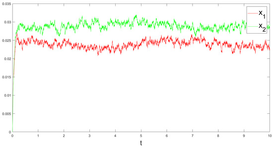
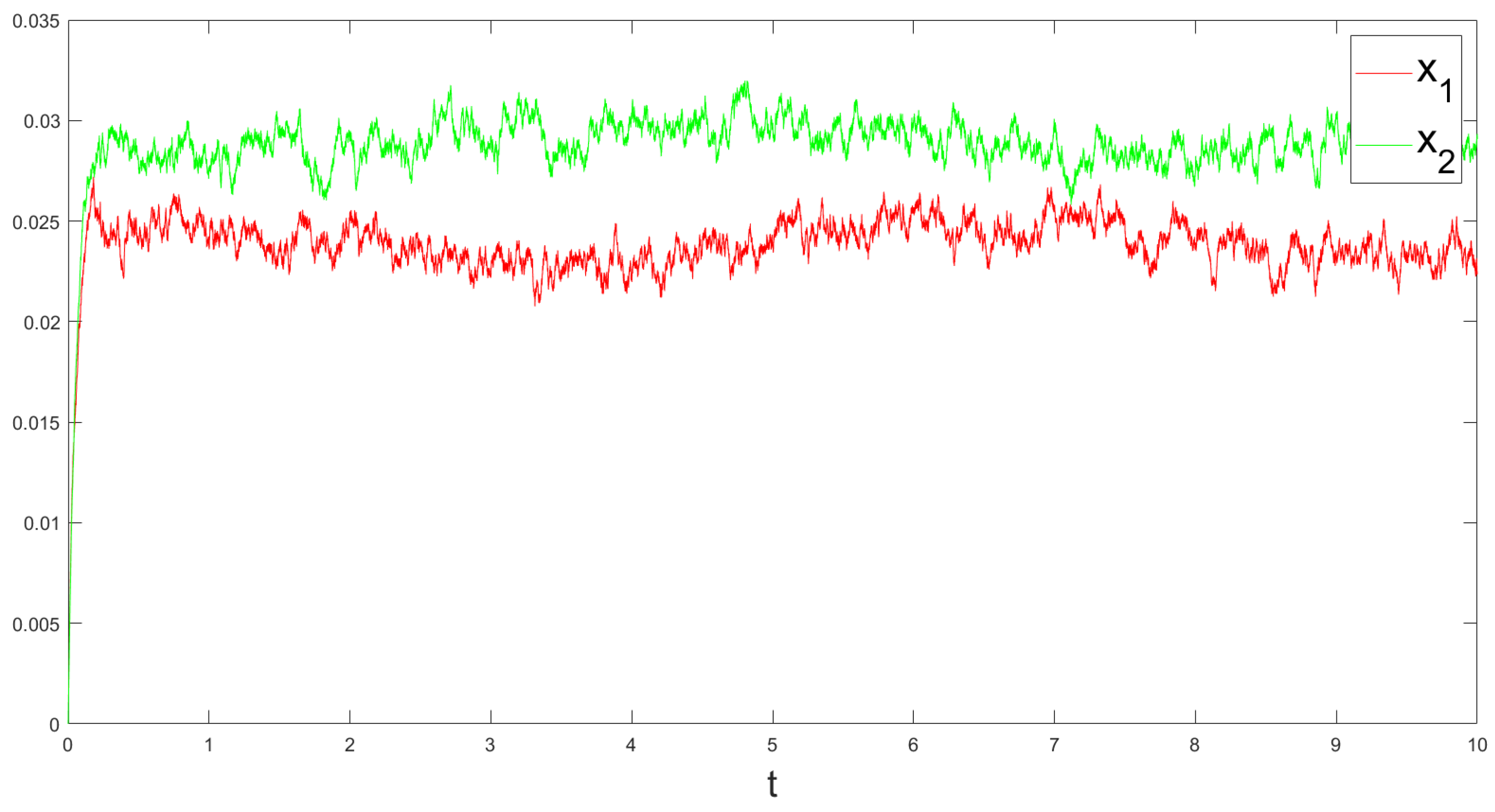
In summary, for the parameters considered here, the requirements of Theorem 1 are met, thereby ensuring the mean-square exponential input-to-state stability of the solution to the Equation (2). The numerical solutions are presented in Figure 1, offering a graphical demonstration that supports the stability of the solution. As observed, the trajectories remain within certain bounds, suggesting that the solution is stable. Nevertheless, it is not guaranteed that they will converge to the equilibrium state.

Example 2.

(3-D case) Consider the 3-D SDRNNs (3) with

$$\begin{array}{cc}\hfill A& =\left[\begin{array}{ccc}-0.234& 0.543& -0.111\\ 0.087& -0.003& 0.764\\ 0.123& 0.456& -0.789\end{array}\right],B=\left[\begin{array}{ccc}0.12& -0.43& 0.75\\ 0.56& 0.08& -0.21\\ -0.33& 0.66& 0.10\end{array}\right],\hfill \\ \hfill C& =\left[\begin{array}{ccc}-0.528& 0.123& 0.876\\ 0.002& -0.439& 0.762\\ -0.111& 0.345& -0.231\end{array}\right],D=\left[\begin{array}{ccc}21& 0& 0\\ 0& 17.2& 0\\ 0& 0& 33.2\end{array}\right].\hfill \end{array}$$

(1) 

Assume that

$$\begin{array}{cc}\hfill & \lambda =0.1,\overline{\tau }=0.9,\rho =1.2,\tau \left(t\right)=0.6cos\left(2t\right)+0.3,L_1=1.32,L_2=0.8,L_3=1.4,\hfill \\ \hfill & \mathbf{f}\left(x_1,x_2,x_3\right)={\left(1.32sin\left(x_1\right),cos\left(x_2\right),-x_3\right)}^T,\hfill \\ \hfill & \mathbf{g}\left(x_1,x_2,x_3\right)={\left(-cos\left(x_1\right),0.61x_2,-0.8x_3\right)}^T,\hfill \\ \hfill & \mathbf{h}\left(x_1,x_2,x_3\right)={\left(x_1,-2sin\left(x_2\right),1.4x_3\right)}^T,\hfill \\ \hfill & \delta \left(\mathbf{x}\left(t\right)\right)=\left(\begin{array}{ccc}0.2x_1\left(t\right)+0.14x_1(t-\overline{\tau })\hfill & 0.02x_2\left(t\right)+0.14x_2(t-\overline{\tau })\hfill & 0.18x_3\left(t\right)\hfill \\ 0.18x_1\left(t\right)+0.01x_1(t-\tau \left(t\right))\hfill & 0.2x_2\left(t\right)+0.11x_2(t-\tau \left(t\right))\hfill & x_3(t-\overline{\tau })\hfill \\ 0.17x_1(t-\overline{\tau })+0.12x_1(t-\tau \left(t\right))\hfill & 0.1x_2(t-\overline{\tau })+0.023x_2(t-\tau \left(t\right))\hfill & x_3(t-\tau \left(t\right))\hfill \end{array}\right),\hfill \\ \hfill & C_1=\left[\begin{array}{ccc}1.2299& -1.2148& -0.7938\\ -1.2148& 2.2408& 0.7683\\ -0.7938& 0.7683& 0.9853\end{array}\right],\hfill \\ \hfill & C_2=\left[\begin{array}{ccc}3.5854& -0.1381& 0.7480\\ -0.1381& 0.4837& -0.1760\\ 0.7480& -0.1760& 1.2145\end{array}\right],\hfill \\ \hfill & C_3=\left[\begin{array}{ccc}1.0982& 0.9260& -0.4042\\ 0.9260& 3.0415& -0.7613\\ -0.4042& -0.7613& 0.8503\end{array}\right].\hfill \end{array}$$

With these selections, Assumption 1 is fulfilled.

(2) 

Define matrices as the following

$$\begin{array}{cc}P=\left[\begin{array}{ccc}1.1559& 0.0913& 0.0952\\ 0.0913& 1.3201& -1.5632\\ 0.0952& -1.5632& 3.1346\end{array}\right],\hfill & \hfill Q=\left[\begin{array}{ccc}31.6731& -0.6097& 3.3026\\ -0.6097& 17.9784& -0.7771\\ 3.3026& -0.7771& 21.2050\end{array}\right],\\ R=\left[\begin{array}{ccc}-364.1912& -20.4426& 8.9232\\ -20.4426& -407.0918& 16.8066\\ 8.9232& 16.8066& -358.7185\end{array}\right],\hfill & \hfill F_1^{\left(1\right)}=\left[\begin{array}{ccc}-1.2000& 0& 0\\ 0& -1.2000& 0\\ 0& 0& -1.2000\end{array}\right],\\ F_1^{\left(2\right)}=\left[\begin{array}{ccc}-1.1000& 0& 0\\ 0& -1.1000& 0\\ 0& 0& -1.1000\end{array}\right],\hfill & \hfill F_1^{\left(3\right)}=\left[\begin{array}{ccc}-1.3000& 0& 0\\ 0& -1.3000& 0\\ 0& 0& -1.3000\end{array}\right],\\ F_2^{\left(1\right)}=\left[\begin{array}{ccc}-0.1865& -0.3530& 1.5343\\ -0.3530& -4.6539& 10.5651\\ 1.5343& 10.5651& -27.7902\end{array}\right],\hfill & \hfill F_2^{\left(2\right)}=\left[\begin{array}{ccc}-10.9870& 10.2946& 3.5284\\ 10.2946& -9.9435& -2.8212\\ 3.5284& -2.8212& -2.8912\end{array}\right],\\ F_2^{\left(3\right)}=\left[\begin{array}{ccc}-1.6881& 2.8188& -0.7869\\ 2.8188& -13.2336& 14.1577\\ -0.7869& 14.1577& -19.7202\end{array}\right].\hfill \end{array}$$

with ${\lambda }^{\left(1\right)}=-31.97,{\lambda }^{\left(2\right)}=-21.84,{\lambda }^{\left(3\right)}=-31.19.$ It follows from the Definition (6) that

$$H_1=\left[\begin{array}{cccccc}-1.2000& 0& 0& -0.2508& 0.6708& -0.1337\\ 0& -1.2000& 0& -0.0988& -0.6672& 2.2318\\ 0& 0& -1.2000& 0.2273& 1.4858& -3.6781\\ -0.2508& -0.0988& 0.2273& -0.1865& -0.3530& 1.5343\\ 0.6708& -0.6672& 1.4858& -0.3530& -4.6539& 10.5651\\ -0.1337& 2.2318& -3.6781& 1.5343& 10.5651& -27.7902\end{array}\right],$$

$$H_2=\left[\begin{array}{cccccc}-1.1000& 0& 0& 0.1584& -0.4269& 0.8573\\ 0& -1.1000& 0& 1.2661& -0.9654& -0.3651\\ 0& 0& -1.1000& -1.8984& 1.9028& 0.7131\\ 0.1584& 1.2661& -1.8984& -10.9870& 10.2946& 3.5284\\ -0.4269& -0.9654& 1.9028& 10.2946& -9.9435& -2.8212\\ 0.8573& -0.3651& 0.7131& 3.5284& -2.8212& -2.8912\end{array}\right],$$

$$H_3=\left[\begin{array}{cccccc}-1.3000& 0& 0& -0.6207& 0.1349& 1.0601\\ 0& -1.3000& 0& 0.1279& -1.1076& 1.4470\\ 0& 0& -1.3000& -0.4013& 1.7794& -1.8319\\ -0.6207& 0.1279& -0.4013& -1.6881& 2.8188& -0.7869\\ 0.1349& -1.1076& 1.7794& 2.8188& -13.2336& 14.1577\\ 1.0601& 1.4470& -1.8319& -0.7869& 14.1577& -19.7202\end{array}\right]$$

It is readily apparent that $H_1,H_2,H_3$ are non-positive definite, thereby confirming that Assumption 2 holds.

(3) 

It can be deduced from (8) that

$$H_4=\left[\begin{array}{ccc}-315.3378& -29.0086& 2.9766\\ -29.7025& -361.8602& 115.8151\\ 5.2995& 65.7927& -469.7871\end{array}\right],H_5=\left[\begin{array}{ccc}-0.5000& 0& 0\\ 0& -0.5000& 0\\ 0& 0& -0.5000\end{array}\right],$$

and $H_6=\left[\begin{array}{ccc}-1& 0& 0\\ 0& -1& 0\\ 0& 0& -1\end{array}\right].$ It can be easily established that $H_4,H_5,H_6$ are non-positive definite.

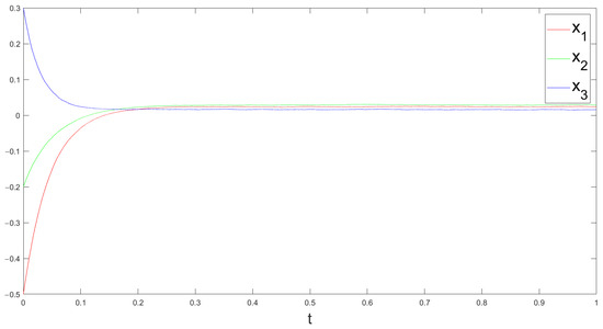
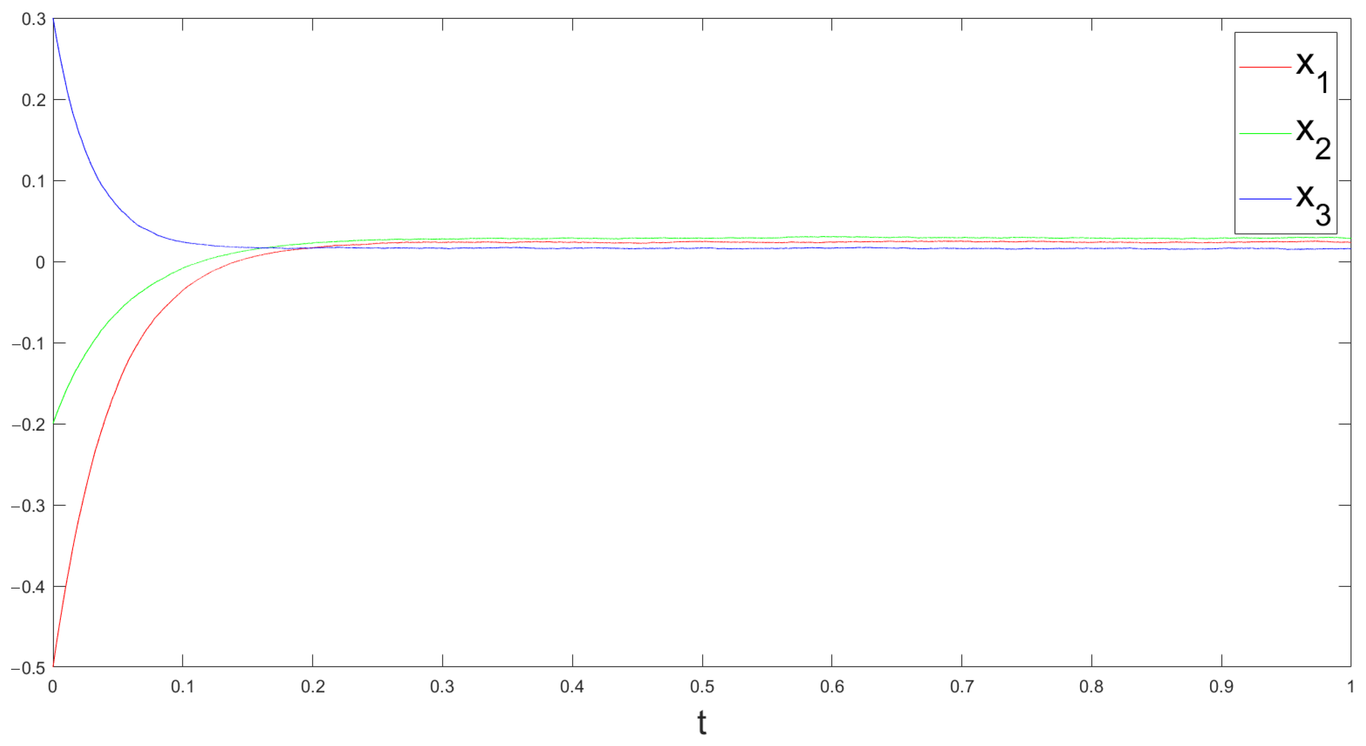
In conclusion, given the parameters under consideration, the conditions of Theorem 4 are satisfied, which guarantees both mean-square exponential stability and almost sure exponential stability for the solution to Equation (3). The numerical solutions illustrated in Figure 2 provide a visual confirmation of the solution’s stability. They reveal that the solution rapidly converges to the equilibrium state, indicating a swift stabilization of the system.

5. Proof of Main Theorems

5.1. Preliminary Lemmas

Let $C^{2,1}\left(R^n\times R_{+};R_{+}\right)$ represent all nonnegative functions $V(\mathbf{X},t)$ defined over $R^n\times R_{+}$ that are twice continuously differentiable with respect to x and once continuously differentiable with respect to t. For every $V\in C^{2,1}\left(R^n,R_{+}\right)$, we introduce an operator $\mathrm{d}V$, which is related to the stochastic delay function (2) as follows:

$$\mathrm{d}V(\mathbf{X}\left(t\right),t)=\mathcal{L}V(\mathbf{X}\left(t\right),t)\mathrm{d}t+V_x(\mathbf{X}\left(t\right),t)\delta \left(\mathbf{X}\left(t\right)\right)\mathrm{d}\mathbf{W}\left(t\right)$$

(10)

with

$$\begin{array}{cc}\hfill \mathcal{L}V\left(\mathbf{X}\right(t),t)& =V_x(\mathbf{X}\left(t\right),t)\left[-D\mathbf{X}\left(t\right)+A\mathbf{f}\left(\mathbf{X}\left(t\right)\right)+B\mathbf{g}\left(\mathbf{X}(t-\overline{\tau })\right)+C\mathbf{h}\left(X(t-\tau \left(t\right))\right)+\mathbf{u}\left(t\right)\right]\hfill \\ & +V_t(\mathbf{X}\left(t\right),t)+{\displaystyle \frac{1}{2}}tr\left[{\sigma }^{\mathrm{T}}\left(\mathbf{X}\left(t\right)\right)V_{\mathrm{xx}}(\mathbf{X}\left(t\right),t)\sigma \left(\mathbf{X}\left(t\right)\right)\right].\hfill \end{array}$$

(11)

Subsequently, we will proceed to estimate $\mathcal{L}V\left(\mathbf{x}\right(t),t)$ for specific Lyapunov functions associated with the stochastic delay function (2).

Lemma 1.

If Assumptions 1 and 2 are satisfied, let ${\lambda }^{\left(1\right)},{\lambda }^{\left(2\right)},{\lambda }^{\left(3\right)}$ be given in Remark 6. Define

$$\begin{array}{cc}\hfill V\left(\mathbf{X}\right(t),t)=& e^{\lambda t}{\mathbf{X}}^T\left(t\right)P\mathbf{X}\left(t\right)+{\int }_{t-\overline{\tau }}^t{e}^{\lambda s}{\mathbf{X}}^T\left(s\right)Q\mathbf{X}\left(s\right)ds+{\int }_{t-\tau \left(t\right)}^t{e}^{\lambda s}{\mathbf{X}}^T\left(s\right)R\mathbf{X}\left(s\right)ds\hfill \end{array}$$

(12)

where $\lambda >0,$ and $P,Q,R$ are $n\times n$ positive matrices. Then, for the trivial solution $\mathbf{x}\left(t\right)$ of Equation (2), the following holds:

$$\begin{array}{c}\hfill \begin{array}{c}\hfill e^{-\lambda t}\mathcal{L}V(\mathbf{X}\left(t\right),t)\le {\mathbf{X}}^T\left(t\right)H_4\mathbf{X}\left(t\right)+{\mathbf{X}}^T(t-\overline{\tau })H_5{\mathbf{X}}^T(t-\overline{\tau })\\ +{\mathbf{X}}^T(t-\tau \left(t\right))H_6{\mathbf{X}}^T(t-\tau \left(t\right))+{\left|\mathbf{u}\left(t\right)\right|}^2.\hfill \end{array}\end{array}$$

(13)

where $H_4,H_5,H_6$ are defined in Equation (8).

Proof. 

Under the assumptions of this lemma, it can be readily inferred from (2), (5) and (12) that

$$\begin{array}{cc}\hfill & V_t(\mathbf{X}\left(t\right),t)⩽e^{\lambda t}{\mathbf{X}}^T\left(t\right)(\lambda P+Q+R)\mathbf{X}\left(t\right)-e^{\lambda t}{e}^{-\lambda \overline{\tau }}{\mathbf{X}}^T(t-\overline{\tau })Q\mathbf{X}(t-\overline{\tau })\hfill \\ \hfill & -e^{\lambda t}{e}^{-\lambda \overline{\tau }}(1-\rho ){\mathbf{X}}^T(t-\tau \left(t\right))R\mathbf{X}(t-\tau \left(t\right)),\hfill \end{array}$$

$$\begin{array}{cc}\hfill & V_{\mathbf{x}}(\mathbf{X}\left(t\right),t)=2e^{\lambda t}{\mathbf{X}}^T\left(t\right)P,\hfill \end{array}$$

$$\begin{array}{cc}\hfill & 2\mathbf{X}{\left(t\right)}^{T}P\left[A\mathbf{f}\left(\mathbf{X}\left(t\right)\right)+B\mathbf{g}\left(\mathbf{X}(t-\overline{\tau })\right)+C\mathbf{h}\left(\mathbf{X}(t-\tau \left(t\right))\right)\right]\hfill \\ \hfill & ={\left(\mathbf{X}\left(t\right),\mathbf{f}\left(\mathbf{X}\right(t\left)\right)\right)}^T\left(\begin{array}{cc}{F}_1^{\left(1\right)}& PA\\ A^T{P}^T& F_2^{\left(1\right)}\end{array}\right)\left(\begin{array}{c}\mathbf{X}\left(t\right)\\ \mathbf{f}\left(\mathbf{X}\right(t\left)\right)\end{array}\right)-{\mathbf{f}}^T\left(\mathbf{X}\left(t\right)\right)F_2^{\left(1\right)}\mathbf{f}\left(\mathbf{X}\left(t\right)\right)\hfill \\ \hfill & +{\left(\mathbf{X}\left(t\right),\mathbf{g}\left(\mathbf{X}(t-\overline{\tau })\right)\right)}^T\left(\begin{array}{cc}{F}_1^{\left(2\right)}& PB\\ B^T{P}^T& F_2^{\left(2\right)}\end{array}\right)\left(\begin{array}{c}\mathbf{X}\left(t\right)\\ \mathbf{g}\left(\mathbf{X}(t-\overline{\tau })\right)\end{array}\right)\hfill \\ \hfill & -{\mathbf{g}}^T\left(\mathbf{X}(t-\overline{\tau })\right)F_2^{\left(2\right)}\mathbf{g}\left(\mathbf{X}(t-\overline{\tau })\right)\hfill \\ \hfill & +{\left(\mathbf{X}\left(t\right),\mathbf{h}\left(\mathbf{X}\right(t-\tau \left(t\right)\left)\right)\right)}^T\left(\begin{array}{cc}{F}_1^{\left(3\right)}& PC\\ C^T{P}^T& F_2^{\left(3\right)}\end{array}\right)\left(\begin{array}{c}\mathbf{X}\left(t\right)\\ \mathbf{h}\left(\mathbf{X}\right(t-\tau \left(t\right)\left)\right)\end{array}\right)\hfill \\ \hfill & -{\mathbf{h}}^T\left(\mathbf{X}(t-\tau \left(t\right))\right)F_2^{\left(3\right)}\mathbf{h}\left(\mathbf{X}(t-\tau \left(t\right))\right)-{\mathbf{X}}^T\left(t\right)\left(F_1^{\left(1\right)}+F_1^{\left(2\right)}+F_1^{\left(3\right)}\right)\mathbf{X}\left(t\right),\hfill \\ \hfill & {\displaystyle \frac{1}{2}}tr\left[{\sigma }^{\mathrm{T}}\left(\mathbf{X}\left(t\right)\right)V_{\mathbf{x}\mathbf{x}}(\mathbf{X}\left(t\right),t)\sigma \left(\mathbf{X}\left(t\right)\right)\right]\hfill \\ \hfill & \le e^{\lambda t}{\lambda }_{max}\left(P\right)\left[{\mathbf{X}}^T\left(t\right)C_1\mathbf{X}\left(t\right)+{\mathbf{X}}^T(t-\overline{\tau })C_2\mathbf{X}(t-\overline{\tau })+{\mathbf{X}}^T(t-\tau \left(t\right))C_3(\mathbf{X}(t-\tau \left(t\right))\right].\hfill \end{array}$$

Combing these results with the fact that $H_1,H_2,H_3$ are symmetric non-positive definite, we get

$$\begin{array}{c}\hfill \begin{array}{c}\mathcal{L}V\left(\mathbf{X}\right(t),t)\hfill \\ \le e^{\lambda t}{\mathbf{X}}^T\left(t\right)\left(P{P}^T+\lambda P+Q+R+{\lambda }_{max}\left(P\right)C_1-2PD-F_1^{\left(1\right)}-F_1^{\left(2\right)}-F_1^{\left(3\right)}\right)\mathbf{X}\left(t\right)\hfill \\ +e^{\lambda t}{\mathbf{X}}^T(t-\overline{\tau })\left({\lambda }_{max}\left(P\right)C_2-e^{-\lambda \overline{\tau }}Q\right){\mathbf{X}}^T(t-\overline{\tau })\hfill \\ +e^{\lambda t}{\mathbf{X}}^T(t-\tau \left(t\right))\left({\lambda }_{max}\left(P\right)C_3-e^{-\lambda \overline{\tau }}(1-\rho )R\right){\mathbf{X}}^T(t-\tau \left(t\right))\hfill \\ +e^{\lambda t}{\left|\mathbf{u}\left(t\right)\right|}^2-e^{\lambda t}{\mathbf{f}}^T\left(\mathbf{X}\left(t\right)\right)F_2^{\left(1\right)}\mathbf{f}\left(\mathbf{X}\left(t\right)\right)\hfill \\ -e^{\lambda t}{\mathbf{g}}^T\left(\mathbf{X}(t-\overline{\tau })\right)F_2^{\left(2\right)}\mathbf{g}\left(\mathbf{X}(t-\overline{\tau })\right)-e^{\lambda t}{\mathbf{h}}^T\left(\mathbf{X}(t-\tau \left(t\right))\right)F_2^{\left(3\right)}\mathbf{h}\left(\mathbf{X}(t-\tau \left(t\right))\right).\hfill \end{array}\end{array}$$

Combining this with the relation (7), we arrive at the conclusion stated in (13). □

To establish almost sure exponential stability for the system (3), we necessitate the following results. The subsequent discussion is inspired by the work presented in [41].

Lemma 2

(Semimartingale convergence theorem [41]). Consider $A_1\left(t\right)$ and $A_2\left(t\right)$ as two continuous, adapted and increasing processes on $t⩾0$ with initial conditions $A_1\left(0\right)=A_2\left(0\right)=0$ almost surely (a.s.). Let $A_3\left(t\right)$ be a real-valued continuous local martingale, also starting at $A_3\left(0\right)=0$ a.s. Let ζ be a nonnegative random variable that is ${\mathcal{F}}_0$-measurable with a finite expected value, $E\left[\zeta \right]<\infty$. Define the process

$$Y\left(t\right)=\zeta +A_1\left(t\right)-A_2\left(t\right)+A_3\left(t\right)\mathit{for}t⩾0.$$

If $Y\left(t\right)$ remains nonnegative, then the following implication holds:

$$\{\underset{t\to \infty }{lim}{A}_1\left(t\right)<\infty \}\subset \{\underset{t\to \infty }{lim}Y\left(t\right)<\infty \}\cap \{\underset{t\to \infty }{lim}{A}_2\left(t\right)<\infty \}a.s.$$

Here, $B_1\subset B_2$ a.s. indicates that the probability of the intersection of $B_1$ and the complement of $B_2$ is zero, $P(B_1\cap B_2^c)=0$. Specifically, if ${lim}_{t\to \infty }{A}_1\left(t\right)<\infty$ a.s., then for almost all outcomes $\omega \in \mathrm{\Omega }$,

$$\underset{t\to \infty }{lim}Y(t,\omega )<\infty \mathit{and}\underset{t\to \infty }{lim}{A}_2(t,\omega )<\infty .$$

This suggests that both the process Y and $A_2$ tend to approach finite random values as $t\to \infty$.

Lemma 3.

Let $\gamma >0$, and let $\psi :R\to R^{+}$ be any continuous function, then

$$\begin{array}{c}\hfill \begin{array}{c}{\int }_0^t{e}^{\gamma s}\psi \left(s-\tau \left(t\right)\right)ds⩽-e^{\gamma \overline{\tau }}{\int }_{t-\tau \left(t\right)}^t{e}^{\gamma s}\psi \left(s\right)ds+e^{\gamma \overline{\tau }}{\int }_{-\overline{\tau }}^0{e}^{\gamma s}\psi \left(s\right)ds+e^{\gamma \overline{\tau }}{\int }_0^t{e}^{\gamma s}\psi \left(s\right)ds\hfill \\ {\int }_0^t{e}^{\gamma s}\psi \left(s-\overline{\tau }\right)ds⩽-e^{\gamma \overline{\tau }}{\int }_{t-\overline{\tau }}^t{e}^{\gamma s}\psi \left(s\right)ds+e^{\gamma \overline{\tau }}{\int }_{-\overline{\tau }}^0{e}^{\gamma s}\psi \left(s\right)ds+e^{\gamma \overline{\tau }}{\int }_0^t{e}^{\gamma s}\psi \left(s\right)ds\hfill \end{array}\end{array}$$

Proof. 

It is sufficient to demonstrate the validity of the first relation, as the second relation is merely a specific instance of the first one. Through direct computation, we arrive at the following result:

$$\begin{array}{c}{\int }_{t-\tau \left(t\right)}^t{e}^{\gamma s}\psi \left(s\right)ds={\int }_{t-\tau \left(t\right)}^{-\tau \left(t\right)}{e}^{\gamma s}\psi \left(s\right)ds+{\int }_{-\tau \left(t\right)}^t{e}^{\gamma s}\psi \left(s\right)ds\hfill \\ ={\int }_t^0{e}^{\gamma (s-\tau (t\left)\right)}\psi (s-\tau \left(t\right))ds+{\int }_{-\tau \left(t\right)}^t{e}^{\gamma s}\psi \left(s\right)ds\hfill \\ ⩽-{\int }_0^t{e}^{-\gamma \overline{\tau }}{e}^{\gamma s}\psi (s-\tau \left(t\right))ds+{\int }_{-\overline{\tau }}^t{e}^{\gamma s}\psi \left(s\right)ds\hfill \end{array}$$

The final equality is valid because $\tau \left(t\right)$ is less than or equal to $\overline{\tau }$ by definition. □

5.2. Theorem Demonstration: A Systematic Exposition of the Proofs

Proof. 

Theorem 5’s proof: Let $V(\mathbf{X},t)$ be defined in accordance with (12), and consider $\mathbf{X}\left(t\right):=\mathbf{X}(t;\mathrm{\Psi })$ to be the solution of Equation (2). When we take into account that $H_4,H_5,H_6$ are all non-positive definite matrices and couple this observation with the conclusions of Lemma 1, we derive the following conclusion:

$$\mathcal{L}V(\mathbf{X}\left(t\right),t)\le e^{\lambda t}{\left|\mathbf{u}\left(t\right)\right|}^2.$$

(14)

Next, we introduce a stopping time

$${\theta }_k:=inf\{t\ge 0:|\mathbf{X}\left(t\right)|\ge k\}$$

It can be inferred from Dynkin’s formula that

$$\mathbf{E}V\left(\mathbf{X}\left(t\wedge {\theta }_k\right),t\wedge {\theta }_k\right)=\mathbf{E}V(\mathbf{X}\left(0\right),0)+\mathbf{E}\left[{\int }_0^{t\wedge {\theta }_k}\mathcal{L}V(X\left(y\right),y)dy\right].$$

(15)

By taking the limit $k\to \infty$ on both sides of Equation (15) and applying the monotone convergence theorem along with Equation (14), we easily derive

$$\begin{array}{c}\hfill \mathbf{E}V(\mathbf{X}\left(t\right),t)\le \mathbf{E}V(\mathbf{X}\left(0\right),0)+{\parallel u\parallel }_{\infty }^2{\int }_0^t{e}^{\lambda y}dy\le {\mathbf{E}\parallel \mathrm{\Psi }\parallel }^2+{\displaystyle \frac{1}{\lambda }}{\parallel u\parallel }_{\infty }^2\left(e^{\lambda t}-1\right).\end{array}$$

Combining this with the definitions provided in (12), we obtain the following result

$$\begin{array}{c}\hfill \begin{array}{c}\hfill e^{\lambda t}{\lambda }_{min}\left(P\right)\mathbf{E}\left({\left|\mathbf{X}\left(t\right)\right|}^2\le e^{\lambda t}\mathbf{E}\left[{\mathbf{X}}^T\left(t\right)P\mathbf{X}\left(t\right)\right]\le \mathbf{E}V(X\left(t\right),t)\right.\\ \hfill \le {\mathbf{E}\parallel \mathrm{\Psi }\parallel }^2+{\displaystyle \frac{1}{\lambda }}{\parallel u\parallel }_{\infty }^2\left(e^{\lambda t}-1\right).\end{array}\end{array}$$

That is,

$$\begin{array}{c}\hfill {\mathbf{E}\left|X\left(t\right)\right|}^2\le e^{-\lambda t}{\displaystyle \frac{{\mathbf{E}\parallel \mathrm{\Psi }\parallel }^2}{{\lambda }_{min}\left(P\right)}}+{\displaystyle \frac{1}{\lambda }}{\displaystyle \frac{{\parallel u\parallel }_{\infty }^2}{{\lambda }_{min}\left(P\right)}}.\end{array}$$

This in conjunction with Definition 1 confirms that the trivial solution of system (2) is mean-square exponentially input-to-state-stable. □

Proof. 

Theorem 3’s proof: Let $V(\mathbf{X},t)$ be defined in (12), and consider $\mathbf{X}\left(t\right):=\mathbf{X}(t;\mathrm{\Psi })$ as the solution to the Equation (3). It follows from Lemma 1 with the assumption $\mathbf{u}\left(t\right)=0$ that

$$\begin{array}{c}\hfill \begin{array}{c}{e}^{-\lambda t}\mathcal{L}V(\mathbf{X}\left(t\right),t)\hfill \\ \le {\mathbf{X}}^T\left(t\right)H_4\mathbf{X}\left(t\right)+{\mathbf{X}}^T(t-\overline{\tau })H_5{\mathbf{X}}^T(t-\overline{\tau })+{\mathbf{X}}^T(t-\tau \left(t\right))H_6{\mathbf{X}}^T(t-\tau \left(t\right)).\hfill \end{array}\end{array}$$

Thus

$$\begin{array}{c}V\left(\mathbf{X}\right(t),t)\hfill \\ \le V(\mathbf{X}\left(0\right),0)+{\int }_0^t{V}_x(\mathbf{X}\left(y\right),y)\delta \left(\mathbf{X}\left(y\right)\right)\mathrm{d}\mathbf{W}\left(y\right)\hfill \\ +{\int }_0^t{e}^{\lambda y}{\mathbf{X}}^T\left(y\right)H_4\mathbf{X}\left(y\right)dy\hfill \\ +{\int }_0^t{e}^{\lambda y}{\mathbf{X}}^T(y-\overline{\tau })H_5\mathbf{X}(y-\overline{\tau })dy\hfill \\ +{\int }_0^t{e}^{\lambda y}{\mathbf{X}}^T(y-\tau \left(y\right))H_6\mathbf{X}(y-\tau \left(y\right))dy.\hfill \end{array}$$

(16)

This together with Lemma 3 implies that

$$\begin{array}{cc}\hfill & {\int }_0^t{e}^{\lambda y}{\mathbf{X}}^T(y-\overline{\tau })H_5\mathbf{X}(y-)dy+{\int }_0^t{e}^{\lambda y}{\mathbf{X}}^T(y-\tau \left(t\right))H_6\mathbf{X}(y-\tau \left(y\right))dy\hfill \\ \hfill & \le -e^{\lambda \overline{\tau }}{\int }_{t-\overline{\tau }}^t{e}^{\lambda y}{\mathbf{X}}^T\left(y\right)H_5\mathbf{X}\left(y\right)dy-e^{\lambda \overline{\tau }}{\int }_{t-\tau \left(t\right)}^t{e}^{\lambda y}{\mathbf{X}}^T\left(y\right)H_6\mathbf{X}\left(y\right)dy\hfill \\ \hfill & +e^{\lambda \overline{\tau }}{\int }_{-\overline{\tau }}^0{e}^{\lambda y}\mathbf{X}\left(y\right)H_5\mathbf{X}\left(y\right)dy+e^{\lambda \overline{\tau }}{\int }_{-\overline{\tau }}^0{e}^{\lambda y}{\mathbf{X}}^T\left(y\right)H_6\mathbf{X}\left(y\right)dy\hfill \\ \hfill & +e^{\lambda \overline{\tau }}{\int }_0^t{e}^{\lambda y}{\mathbf{X}}^T\left(y\right)H_5\mathbf{X}\left(y\right)dy+e^{\lambda \overline{\tau }}{\int }_0^t{e}^{\lambda y}{\mathbf{X}}^T\left(y\right)H_6\mathbf{X}\left(y\right)dy\hfill \end{array}$$

(17)

Combining relation (16) and (17), we have

$$\begin{array}{cc}\hfill V\left(\mathbf{X}\right(t),t)& \le V(\mathbf{X}\left(0\right),0)+{\int }_0^t{V}_x(\mathbf{X}\left(y\right),y)\delta \left(x\left(y\right)\right)\mathrm{d}\mathbf{W}\left(y\right)\hfill \\ \hfill & +{\int }_0^t{e}^{\lambda y}{\mathbf{X}}^T\left(y\right)H_4\mathbf{X}\left(y\right)dy\hfill \\ \hfill & -e^{\lambda \overline{\tau }}{\int }_{t-\overline{\tau }}^t{e}^{\lambda y}{\mathbf{X}}^T\left(y\right)H_5\mathbf{X}\left(y\right)dy-e^{\lambda \overline{\tau }}{\int }_{t-\tau \left(t\right)}^t{e}^{\lambda y}{\mathbf{X}}^T\left(y\right)H_6\mathbf{X}\left(y\right)dy\hfill \\ \hfill & +e^{\lambda \overline{\tau }}{\int }_{-\overline{\tau }}^0{e}^{\lambda y}{\mathbf{X}}^T\left(y\right)H_5\mathbf{X}\left(y\right)dy+e^{\lambda \overline{\tau }}{\int }_{-\overline{\tau }}^0{e}^{\lambda y}{\mathbf{X}}^T\left(y\right)H_6\mathbf{X}\left(y\right)dy\hfill \\ \hfill & +e^{\lambda \overline{\tau }}{\int }_0^t{e}^{\lambda y}{\mathbf{X}}^T\left(y\right)H_5\mathbf{X}\left(y\right)dy+e^{\lambda \overline{\tau }}{\int }_0^t{e}^{\lambda y}{\mathbf{X}}^T\left(y\right)H_6\mathbf{X}\left(y\right)dy\hfill \end{array}$$

(18)

thus

$$\begin{array}{c}V(\mathbf{X}\left(t\right),t)+e^{\lambda \overline{\tau }}{\int }_{t-\overline{\tau }}^t{e}^{\lambda y}{\mathbf{X}}^T\left(y\right)H_5\mathbf{X}\left(y\right)dy+e^{\lambda \overline{\tau }}{\int }_{t-\tau \left(t\right)}^t{e}^{\lambda y}{\mathbf{X}}^T\left(y\right)H_6\mathbf{X}\left(y\right)dy\hfill \\ \le V(\mathbf{X}\left(0\right),0)+{\int }_0^t{V}_x(\mathbf{X}\left(y\right),y)\delta \left(\mathbf{X}\left(y\right)\right)\mathrm{d}\mathbf{W}\left(y\right)\hfill \\ +e^{\lambda \overline{\tau }}{\int }_{-\overline{\tau }}^0{e}^{\lambda y}{\mathbf{X}}^T\left(y\right)H_5\mathbf{X}\left(y\right)dy+e^{\lambda \overline{\tau }}{\int }_{-\overline{\tau }}^0{e}^{\lambda y}{\mathbf{X}}^T\left(y\right)H_6\mathbf{X}\left(y\right)dy\hfill \\ +{\int }_0^t{e}^{\lambda y}{\mathbf{X}}^T\left(y\right)\left(H_4+e^{\lambda \overline{\tau }}{H}_5+e^{\lambda \overline{\tau }}{H}_6\right)\mathbf{X}\left(y\right)dy\hfill \end{array}$$

(19)

Making use of (19) and the non-positiveness of $H_4+e^{\gamma \overline{\tau }}(H_5+H_6)$ yields that

$$\begin{array}{c}V(\mathbf{X}\left(t\right),t)+e^{\lambda \overline{\tau }}{\int }_{t-\overline{\tau }}^t{e}^{\lambda y}{\mathbf{X}}^T\left(y\right)H_5\mathbf{X}\left(y\right)dy+e^{\lambda \overline{\overline{\tau }}}{\int }_{t-\tau \left(t\right)}^t{e}^{\lambda y}{\mathbf{X}}^T\left(y\right)H_6\mathbf{X}\left(y\right)dy\hfill \\ \le Y\left(t\right)\hfill \end{array}$$

(20)

where

$$\begin{array}{c}\hfill \begin{array}{cc}Y\left(t\right)\hfill & =V(\mathbf{X}\left(0\right),0)+{\int }_0^t{U}_x(\mathbf{X}\left(y\right),y)\delta \left(\mathbf{X}\left(y\right)\right)\mathrm{d}W\left(y\right)\hfill \\ \hfill & +e^{\lambda \overline{\tau }}{\int }_{-\overline{\tau }}^0{e}^{\lambda y}{\mathbf{X}}^T\left(y\right)H_5\mathbf{X}\left(y\right)dy+e^{\lambda \overline{\tau }}{\int }_{-\overline{\tau }}^0{e}^{\lambda y}{\mathbf{X}}^T\left(y\right)H_6\mathbf{X}\left(y\right)dy\hfill \end{array}\end{array}$$

which constitutes a nonnegative martingale, and Lemma 2 demonstrates that

$$\underset{s\to \infty }{lim}Y\left(s\right)<\infty \mathrm{a}.\mathrm{s}.$$

Consequently, Equation (20) leads to

$$\underset{s\to \infty }{lim\; sup}\left[V\left(\mathbf{X}\right(s),s)\right]<\infty \mathrm{a}.\mathrm{s}..$$

This together with the fact that

$$\begin{array}{c}\hfill e^{\lambda t}{\lambda }_{min}\left(P\right){\left|\mathbf{X}\left(t\right)\right|}^2\le e^{\lambda t}{\mathbf{X}}^T\left(t\right)P\mathbf{x}\left(t\right)\le V(\mathbf{X}\left(t\right),t).\end{array}$$

implies that

$$\underset{s\to \infty }{lim\; sup}{\displaystyle \frac{1}{s}}log\left({\left|\mathbf{X}\left(t\right)\right|}^2\right)\le \underset{s\to \infty }{lim\; sup}{\displaystyle \frac{1}{s}}log\left(V(\mathbf{X}\left(s\right),s)\right)⩽-\lambda \mathrm{a}.\mathrm{s}.$$

which is equivalent to (9). □

6. Conclusions

The investigation conducted in this research, employing a matrix-based methodology, has successfully demonstrated the stability of solutions for SDRNNs. Our findings rest on less restrictive assumptions compared to scalar methods and yield a broader range of stability conclusions. Beyond enhancing the mean-square exponential input-to-state stability results previously introduced in [36], we have also provided insights into mean-square exponential stability and almost sure exponential stability for cases with no input. The effectiveness of our theoretical results has been confirmed through numerical simulations, highlighting their practical applicability.

While our work focuses on theoretical stability analysis, future research could explore several promising directions. First, extending our analysis to more general system configurations, such as those with different types of time-varying delays or noise structures, would further broaden the applicability of the results. Second, developing efficient numerical methods to compute the controller parameters based on the derived stability conditions could bridge the gap between theory and practical implementation. Third, investigating the resilience of SDRNNs to parameter uncertainties and external disturbances would enhance the robustness of the stability results. These future directions align with the growing demand for more sophisticated and reliable neural network models in real-world applications.

References

- Duan, L.; Ren, Y.; Duan, F. Adaptive stochastic resonance based convolutional neural network for image classification. Chaos Solitons Fractals 2022, 162, 112429. [Google Scholar] [CrossRef]
- Morán, A.; Parrilla, L.; Roca, M.; Font-Rossello, J.; Isern, E.; Canals, V. Digital implementation of radial basis function neural networks based on stochastic computing. IEEE J. Emerg. Sel. Top. Circuits Syst. 2022, 13, 257–269. [Google Scholar] [CrossRef]
- Hofmann, D.; Fabiani, G.; Mentink, J.H.; Carleo, G.; Sentef, M.A. Role of stochastic noise and generalization error in the time propagation of neural-network quantum states. Scipost Phys. 2022, 12, 165. [Google Scholar] [CrossRef]
- Yamakou, M.E.; Zhu, J.; Martens, E.A. Inverse stochastic resonance in adaptive small-world neural networks. Chaos Interdiscip. J. Nonlinear Sci. 2024, 34, 113119. [Google Scholar] [CrossRef] [PubMed]
- Sun, Y.; Liang, F. A kernel-expanded stochastic neural network. J. R. Stat. Soc. Ser. B Stat. Methodol. 2022, 84, 547–578. [Google Scholar] [CrossRef]
- Joya, G.; Atencia, M.A.; Sandoval, F. Hopfield neural networks for optimization: Study of the different dynamics. Neurocomputing 2022, 43, 219–237. [Google Scholar] [CrossRef]
- Yang, J.; Ma, L.; Chen, L. L2–L∞ state estimation for continuous stochastic delayed neural networks via memory event-triggering strategy. Int. J. Syst. Sci. 2022, 53, 2742–2757. [Google Scholar] [CrossRef]
- Yang, L.; Gao, T.; Lu, Y.; Duan, J.; Liu, T. Neural network stochastic differential equation models with applications to financial data forecasting. Appl. Math. Model. 2023, 115, 279–299. [Google Scholar] [CrossRef]
- Yang, X.; Deng, W.; Yao, J. Neural network based output feedback control for DC motors with asymptotic stability. Mech. Syst. Signal Process. 2022, 164, 108288. [Google Scholar] [CrossRef]
- Yuan, H.; Zhu, Q. The well-posedness and stabilities of mean-field stochastic differential equations driven by G-Brownian motion. SIAM J. Control Optim. 2025, 63, 596–624. [Google Scholar] [CrossRef]
- McAllister, D.R.; Rawlings, J.B. Nonlinear stochastic model predictive control: Existence, measurability, and stochastic asymptotic stability. IEEE Trans. Autom. Control 2022, 68, 1524–1536. [Google Scholar] [CrossRef]
- Xu, W.; Chen, R.; Li, X. Infinitely deep bayesian neural networks with stochastic differential equations. Int. Conf. Artif. Intell. Stat. 2022, 721–738. [Google Scholar]
- Zhao, Y.; Wang, L. Practical exponential stability of impulsive stochastic food chain system with time-varying delays. Mathematics 2022, 11, 147. [Google Scholar] [CrossRef]
- Zhu, Q. Event-triggered sampling problem for exponential stability of stochastic nonlinear delay systems driven by Levy processes. IEEE Trans. Autom. Control 2025, 70, 1176–1183. [Google Scholar] [CrossRef]
- Zhu, Q.; Cao, J. Robust exponential stability of Markovian jump impulsive stochastic Cohen-Grossberg neural networks with mixed time delays. IEEE Trans. Neural Netw. Learn. Syst. 2010, 21, 1314–1325. [Google Scholar]
- Tran, K.Q.; Nguyen, D.H. Exponential stability of impulsive stochastic differential equations with Markovian switching. Syst. Control Lett. 2022, 162, 105178. [Google Scholar] [CrossRef]
- Xu, H.; Zhu, Q. New criteria on pth moment exponential stability of stochastic delayed differential systems subject to average-delay impulses. Syst. Control Lett. 2022, 164, 105234. [Google Scholar] [CrossRef]
- Li, Z.; Xu, L.; Ma, W. Global attracting sets and exponential stability of stochastic functional differential equations driven by the time-changed Brownian motion. Syst. Control Lett. 2022, 160, 105103. [Google Scholar] [CrossRef]
- Zhu, Q.; Cao, J. Exponential stability analysis of stochastic reaction-diffusion Cohen-Grossberg neural networks with mixed delays. Neurocomputing 2011, 74, 3084–3091. [Google Scholar] [CrossRef]
- Zhu, Q.; Li, X.; Yang, X. Exponential stability for stochastic reaction-diffusion BAM neural networks with time-varying and distributed delays. Appl. Math. Comput. 2011, 217, 6078–6091. [Google Scholar] [CrossRef]
- Liu, Y.; Xu, J.; Lu, J.; Gui, W. Stability of stochastic time-delay systems involving delayed impulses. Automatica 2023, 152, 110955. [Google Scholar] [CrossRef]
- Kechiche, D.; Khemmoudj, A.; Medjden, M. Exponential stability result for the wave equation with Kelvin-Voigt damping and past history subject to Wentzell boundary condition and delay term. Math. Methods Appl. Sci. 2023, 47, 1546–1576. [Google Scholar] [CrossRef]
- Zhang, J.; Nie, X. Coexistence and locally exponential stability of multiple equilibrium points for fractional-order impulsive control Cohen-Grossberg neural networks. Neurocomputing 2024, 589, 127705. [Google Scholar] [CrossRef]
- Zhu, D.; Zhu, Q. Almost sure exponential stability of stochastic nonlinear semi-Markov jump T-S fuzzy systems under intermittent EDF scheduling controller. J. Frankl. Inst. 2024, 361, 107188. [Google Scholar] [CrossRef]
- Liu, X.; Cheng, P. Almost sure exponential stability and stabilization of hybrid stochastic functional differential equations with Lévy noise. J. Appl. Math. Comput. 2023, 69, 3433–3458. [Google Scholar] [CrossRef]
- Pan, L.; Cao, J. Input-to-state Stability of Impulsive Stochastic Nonlinear Systems Driven by G-Brownian Motion. Int. J. Control Autom. Syst. 2021, 19, 1–10. [Google Scholar] [CrossRef]
- Li, X.; Zhang, T.; Wu, J. Input-to-State Stability of Impulsive Systems via Event-Triggered Impulsive Control. IEEE Trans. Cybern. 2022, 52, 7187–7195. [Google Scholar] [CrossRef] [PubMed]
- Liu, S.; Russo, A. Further characterizations of integral input-to-state stability for hybrid systems. Automatica 2024, 163, 111484. [Google Scholar] [CrossRef]
- Yang, X.; Zhao, T.; Zhu, Q. Aperiodic event-triggered controls for stochastic functional differential systems with sampled-data delayed output. IEEE Trans. Autom. Control 2025, 70, 2090–2097. [Google Scholar] [CrossRef]
- Huang, F.; Gao, S. Stochastic integral input-to-state stability for stochastic delayed networked control systems and its applications. Commun. Nonlinear Sci. Numer. Simul. 2024, 138, 108177. [Google Scholar] [CrossRef]
- Xu, G.; Bao, H. Further results on mean-square exponential input-to-state stability of time-varying delayed BAM neural networks with Markovian switching. Neurocomputing 2020, 376, 191–201. [Google Scholar] [CrossRef]
- Song, Q.; Zhao, Z.; Liu, Y.; Alsaadi, F. Mean-square input-to-state stability for stochastic complex-valued neural networks with neutral delay. Neurocomputing 2021, 470, 269–277. [Google Scholar] [CrossRef]
- Wu, K.; Ren, M.; Liu, X. Exponential input-to-state stability of stochastic delay reaction-diffusion neural networks. Neurocomputing 2020, 412, 399–405. [Google Scholar] [CrossRef]
- Wang, W. Mean-square exponential input-to-state stability of stochastic delayed recurrent neural networks with local Lipschitz condition. Math. Methods Appl. Sci. 2023, 46, 17788–17797. [Google Scholar] [CrossRef]
- Radhika, T.; Chandrasekar, A.; Vijayakumar, V.; Zhu, Q. Analysis of Markovian Jump Stochastic Cohen–Grossberg BAM Neural Networks with Time Delays for Exponential Input-to-State Stability. Neural Process. Lett. 2023, 55, 11055–11072. [Google Scholar] [CrossRef]
- Zhu, Q.; Cao, J. Mean-square exponential input-to-state stability of stochastic delayed neural networks. Neurocomputing 2014, 131, 157–163. [Google Scholar] [CrossRef]
- Mao, X. Stochastic Differential Equations and Applications, 2nd ed.; Woodhead Publishing: Cambridge, UK, 2007. [Google Scholar]
- Gikhman, I.; Skorochod, A.V. Stochastic Differential Equations (SDEs); Naukova Dumka, Kiev, 1968; English and German Translation; Springer: Berlin/Heidelberg, Germany, 1971. (in Russian) [Google Scholar]
- Schurz, H. Basic concepts of numerical analysis of stochastic differential equations explained by balanced implicit theta methods. In Stochastic Differential Equations and Processes; Mounir, Z., Filatova, D.V., Eds.; Springer Proceedings in Mathematics 7; Springer: New York, NY, USA, 2012; pp. 1–139. [Google Scholar]
- Graham, C.; Talay, D. Discretization of Stochastic Differential Equations. Stochastic Simulation and Monte Carlo Methods. In Mathematical Foundations of Stochastic Simulation; Springer: New York, NY, USA, 2013; pp. 155–195. [Google Scholar]
- Liptser, R.S.; Shiryaev, A.N. Statistics of Random Processes I: General Theory, 2nd ed.; Springer: Berlin/Heidelberg, Germany, 1989. [Google Scholar]
Disclaimer/Publisher’s Note: The statements, opinions and data contained in all publications are solely those of the individual author(s) and contributor(s) and not of MDPI and/or the editor(s). MDPI and/or the editor(s) disclaim responsibility for any injury to people or property resulting from any ideas, methods, instructions or products referred to in the content. |
© 2025 by the authors. Licensee MDPI, Basel, Switzerland. This article is an open access article distributed under the terms and conditions of the Creative Commons Attribution (CC BY) license (https://creativecommons.org/licenses/by/4.0/).