Robust Variable Selection via Bayesian LASSO-Composite Quantile Regression with Empirical Likelihood: A Hybrid Sampling Approach

Abstract

Since the advent of composite quantile regression (CQR), its inherent robustness has established it as a pivotal methodology for high-dimensional data analysis. High-dimensional outlier contamination refers to data scenarios where the number of observed dimensions (p) is much greater than the sample size (n) and there are extreme outliers in the response variables or covariates (e.g., p/n > 0.1). Traditional penalized regression techniques, however, exhibit notable vulnerability to data outliers during high-dimensional variable selection, often leading to biased parameter estimates and compromised resilience. To address this critical limitation, we propose a novel empirical likelihood (EL)-based variable selection framework that integrates a Bayesian LASSO penalty within the composite quantile regression framework. By constructing a hybrid sampling mechanism that incorporates the Expectation–Maximization (EM) algorithm and Metropolis–Hastings (M-H) algorithm within the Gibbs sampling scheme, this approach effectively tackles variable selection in high-dimensional settings with outlier contamination. This innovative design enables simultaneous optimization of regression coefficients and penalty parameters, circumventing the need for ad hoc selection of optimal penalty parameters—a long-standing challenge in conventional LASSO estimation. Moreover, the proposed method imposes no restrictive assumptions on the distribution of random errors in the model. Through Monte Carlo simulations under outlier interference and empirical analysis of two U.S. house price datasets, we demonstrate that the new approach significantly enhances variable selection accuracy, reduces estimation bias for key regression coefficients, and exhibits robust resistance to data outlier contamination.

1. Introduction

Since Zou and Yuan [1] introduced composite quantile regression (CQR) estimation in 2008, it has emerged as an indispensable tool for high-dimensional data analysis. By aggregating information from multiple quantile points, CQR significantly enhances the robustness of parameter estimates. Huang and Chen [2] laid the groundwork for Bayesian inference in CQR by constructing the first Bayesian hierarchical framework, enabling adaptive parameter estimation through Markov chain Monte Carlo (MCMC) sampling. Subsequent studies have expanded the application scope of CQR: Wang et al. [3] incorporated CQR into right-censored data analysis, integrating local polynomial methods to address heteroskedasticity; Liu et al. [4] proposed a weighted estimation approach for handling missing covariates under random missingness, demonstrating its statistical efficiency in large-sample scenarios. However, conventional CQR methods rely on distributional assumptions of the target variable, which may compromise model accuracy when real-world data deviate from these assumptions.

In contrast, Owen’s empirical likelihood (EL) technique [5,6,7] offers a distribution-free alternative, drawing statistical inferences directly from data. This nonparametric property endows EL with superior robustness against outliers and missing data. Zhao et al. [8] pioneered the application of EL in CQR estimation, establishing its large-sample consistency. Nevertheless, the classical EL approach faces two limitations: it demands substantial data for accurate estimation in complex models, and its parameter estimates often exhibit high variance due to the lack of distributional assumptions, thereby reducing statistical efficiency.

The integration of Bayesian inference with EL has revolutionized quantile regression estimation. The Bayesian empirical likelihood (BEL) framework combines prior distributions with the EL method, enhancing estimation efficiency and resilience in small-sample and missing-data scenarios while enabling more precise parameter inference. Lazar [9] first adapted EL to the Bayesian paradigm, developing the BEL method and demonstrating its efficiency. Fang and Mukerjee [10] further established its higher-order asymptotic properties. Yang and He [11] introduced BEL inference within quantile regression models, using EL as the likelihood function. Subsequent research extended BEL to various models: Zhang and Tang [12] applied it in quantile structural equation models; Chaudhuri et al. [13] optimized sampling efficiency by integrating the Hamiltonian Monte Carlo algorithm. Vexler et al. [14] proposed a BEL method based on quantile comparisons, while Zhao et al. [15] developed BEL-based model selection procedures for complex survey data. These studies collectively highlight BEL’s superiority over classical EL, especially when prior knowledge is available or data quantity is limited. Dong et al. [16] extended the BEL method to the Buckley-James (B-J) estimation model based on censored data and proved the superiority of the method not only in point estimation and confidence interval coverage through simulation analysis, Bedoui and Lazar [17] proposed a semiparametric method for BEL construction based on the Ridge model and the LASSO model and solved the diffusivity in the model by constructing the Metropolis–Hastings (M-H) algorithm. Zhang and Wang [18] applied the BEL method for parameter estimation in the generalized binomial AR (1) model and proved that the method is not only robust but also has faster convergence through numerical simulation and example analysis. Sheng and Ying [19] applied the BEL method for the estimation of the quantile regression model in the absence of observations and argued that the BEL method shows obvious advantages over the classical empirical likelihood method and demonstrated that the BEL method can be applied to the quantile regression model and estimation method and demonstrated the effectiveness of the method. Given that the BEL method shows obvious advantages over the classical empirical likelihood method when the amount of data is limited or prior knowledge is available, the composite quantile regression method has stronger adaptability in dealing with the unknown error distribution compared with the ordinary quantile regression method and the least squares method. Therefore, if the BEL method is extended to composite quantile regression estimation, the robustness and accuracy of estimation can be greatly improved.

The exponential growth of high-dimensional and ultra-high-dimensional data has rendered traditional regression methods inadequate, elevating variable selection to a central challenge in data analysis. In this paper, “outlier pollution” refers specifically to extreme values of the response variable Y in high-dimensional data caused by measurement errors or biased data generation mechanisms (e.g., |Y − median(Y)| > 3σ), which distort the variable selection path of traditional penalized regression. Popular penalized regression techniques, such as LASSO [20], SCAD [21], Adaptive LASSO [22], and Elastic Nets [23], compress regression coefficient vectors to obtain sparse solutions. Meanwhile, Bayesian variable selection methods, initially proposed by Mitchell [24], have gained traction due to their ability to balance model complexity and predictive performance, due to their advantage of maintaining the predictive efficacy of the model while realizing variable dimensionality reduction [25,26,27,28,29,30]. Luo and Li [31,32] systematically investigated Bayesian variable selection in quantile regression, addressing the “curse of dimensionality.” Extensions to survival analysis [21,22,33,34,35,36,37,38] have also yielded fruitful results, exemplified by Li’s [39] innovative penalized likelihood framework for clustered data. Xi et al. [40] integrated the “spike-and-slab” prior into BEL for quantile regression variable selection, while Li [41] demonstrated BEL’s robustness in interval-censored data.

Despite these advancements, the traditional EL method struggles with dimensional adaptation in high-dimensional settings. The penalized empirical likelihood (PEL) approach, proposed by Tang and Leng [42], overcomes this limitation by fusing penalty functions with EL, enabling adaptive variable selection without prespecifying variance structures. The method not only inherits the nonparametric advantage of the empirical likelihood method in confidence interval construction but also demonstrates the statistical efficiency and computational feasibility in high-dimensional scenarios [43,44]. Bayati et al. [45] extended PEL to the Bayesian framework, laying the theoretical foundation for Bayesian PEL. Subsequent studies, including Chul and Adel’s [46] combination of elastic net penalties with Hamiltonian Monte Carlo sampling and Liya’s team’s [47] algorithmic optimizations, have further expanded its applicability.

Notably, despite extensive research on BEL and variable selection, few studies have explored adding penalty terms to the EL function for variable selection within the Bayesian framework. This study bridges this gap by constructing a novel BEL-based CQR method. Leveraging CQR’s robustness, we incorporate a Bayesian LASSO penalty to simultaneously select and estimate key regression coefficients. This approach mitigates the impact of outliers in high-dimensional data, eliminates the need for distributional assumptions about random errors, and circumvents the challenge of optimizing penalty parameters.

2. Modeling and Sparse Optimization Framework

2.1. BEL Variable Selection Algorithm Based on Spike-and-Slab Prior

Let the random sample $(X_i,Y_i),i=1,\dots n$ satisfy the following linear regression model:

$$Y_i=X_i^T\beta +{\epsilon }_i,i=1,\dots ,n$$

(1)

where $\beta ={\left({\beta }_1,\dots ,{\beta }_p\right)}^T$ is the $p\times 1$ dimensional vector of regression coefficients, $X_i$ is a covariant variable, $Y_i$ is the response variable, and suppose there is a component locus of ${\tau }_k=k/(K+1)$. The quantile ${\tau }_k$ of the random error $\epsilon$ is $b_k$, $k=1,2,\dots ,K$. The composite quantile regression estimates of $\beta$ and $(b_1,\dots ,b_K)$ are then obtained by solving the following equation:

$$({\widehat{b}}_1,\dots ,{\widehat{b}}_K,\beta )=\underset{\stackrel{\wedge }{b_1},\dots ,\stackrel{\wedge }{b_K},\beta }{\arg \min }{\displaystyle \sum _{k=1}^K\left\{{\displaystyle \sum _{i=1}^n{\rho }_{{\tau }_k}(Y_i-b_k-X_i^T\beta )}\right\}}$$

(2)

where the loss function is ${\rho }_{{\tau }_k}(x)={\tau }_{k}xI(x\ge 0)+(1-{\tau }_k)xI(x<0)$.

It is easily proven by the following:

$$E\left\{{\tau }_k-I(Y_i-X_i^T\beta \le b_k)\left|X_i\right.\right\}=0$$

(3)

where $I\left(\cdot \right)$ is the indicator function.

Introducing auxiliary random vectors, written as follows:

$${\eta }_i(\beta )={\displaystyle \sum _{k=1}^K{X}_i\left[{\tau }_k-I(Y_i-X_i^T\beta \le b_k)\right]}$$

(4)

which is the estimating function of the composite quantile regression, and thus the empirical likelihood function of the composite quantile regression for model (1) is as follows:

$$L(\beta \left|X,Y\right.)=\sup \left\{{\displaystyle \prod _{i=1}^n{p}_i\left|p_i\ge 0\right.},{\displaystyle \sum _{i=1}^n{p}_i=1,{\displaystyle \sum _{i=1}^n{p}_i{\eta }_i(\beta )=0}}\right\}$$

In order to obtain a sparse solution of the above empirical likelihood function from a Bayesian perspective in the high-dimensional case, we can consider imposing a Spike-and-slab prior on ${\beta }_j,j=1,\dots ,p$ based on the empirical likelihood model $\pi ({\beta }_j\left|{\theta }_j,{\sigma }^2\right.)$, written as follows:

$${\beta }_j\left|{\theta }_j,{\sigma }^2\right.~{\theta }_j{I}_{\{{\beta }_j=0\}}+(1-{\theta }_j)I_{\{{\beta }_j\ne 0\}}N(0,{\sigma }^2)$$

(5)

$${\theta }_j~\mathrm{U}(0,1),j=1,\dots ,p,$$

$$\eta ={\sigma }^{-2}~\Gamma (a,b), a>0,b>0$$

where ${\theta }_j$ and ${\sigma }^2$ are hyperparameters, $\eta ={\sigma }^{-2}$. The super-priors of ${\theta }_j$ and $\eta$ are chosen to be uniform and gamma distributions, respectively, the posterior conditional distributions of the unknown parameters can then be obtained as follows:

$$f(\beta ,\theta ,\eta \left|X,Y\right.;\alpha ,\eta )\propto L(\beta \left|X,Y\right.){\displaystyle \prod _{j=1}^p\pi ({\beta }_j{\left|\theta \right.}_j)}{I}_{(0,1)}({\theta }_j)\Gamma (a,b)$$

(6)

For the above equation, we can consider Gibbs algorithm for sampling estimation of unknown parameters in the model. Let $H=\{j:{\beta }_j\ne 0\}$, $h=\#H$, then the posterior conditional distribution of $\eta$ is as follows:

$$f(\eta \left|\beta ,\theta ,X,Y\right.)\propto \pi (\eta ){\displaystyle \prod _{j=1}^p\pi ({\beta }_j{\left|\theta \right.}_j,\eta )}$$

$$\propto {(\eta )}^{\alpha -1}\exp (-b\eta ){\displaystyle \prod _{j=1}^p[{\theta }_j{I}_{\{{\beta }_j=0\}}+(1-{\theta }_j)I_{\{{\beta }_j\ne 0\}}\frac{1}{\sqrt{2\pi {\eta }^{-1}}}\exp (-\frac{{\beta }_j^2}{2}\eta )]}$$

$$\propto {(\eta )}^{\alpha +h/2-1}\exp (-(b+{\displaystyle \frac{1}{2}}{\displaystyle \sum _{j\in H}{\beta }_j})\eta )$$

(7)

Therefore, the full conditional distribution of $\eta$ obeys $\Gamma (a+0.5h,b+{\displaystyle \frac{1}{2}}{\displaystyle \sum _{j\in H}{\beta }_j^2})$.

The posterior conditional distribution of ${\theta }_j$ is as follows:

$$f({\theta }_j\left|\beta ,{\theta }_{-j},\eta ,X,Y\right.)\propto \pi ({\beta }_j{\left|\theta \right.}_j,\eta )\pi ({\theta }_j)$$

$$\propto [{\theta }_j{I}_{\{{\beta }_j=0\}}+(1-{\theta }_j)I_{\{{\beta }_j\ne 0\}}{\displaystyle \frac{1}{\sqrt{2\pi {\eta }^{-1}}}}\exp (-{\displaystyle \frac{{\beta }_j^2}{2}}\eta )]I_{(0,1)}({\theta }_j)$$

(8)

where ${\beta }_{-j}$ is the sub-vector of $\beta$ minus the j-th element and ${\theta }_{-j}$ is the sub-vector of $\theta$ minus the j-th element. The posterior conditional distribution obtained by Equation (8) obeys $Beta(1+I_{\{{\beta }_j=0\}},1-I_{\{{\beta }_j\ne 0\}})$.

The posterior conditional distribution of ${\beta }_j$ is as follows:

$$f({\beta }_j\left|X,Y\right.,\theta ,\eta ,{\beta }_{-j})\propto L(\beta \left|X,Y\right.)\pi ({\beta }_j{\left|\theta \right.}_j,\eta )$$

(9)

Due to the complex form of Equation (9), it is not possible to sample directly from it, and to overcome this difficulty, M-H arithmetic sampling can be nested in the Gibbs sampler with the following algorithm:

(1)

Let t = 0 and the initial value ${\beta }^{(0)}={\widehat{\beta }}_{\widehat{G}}$;

(2)

Given ${\beta }^{(t)}$, generate ${\eta }^{(t+1)}$ from $\Gamma (a+0.5h,b+{\displaystyle \frac{1}{2}}{\displaystyle \sum _{j\in H}{\beta }_j^2})$, where $H=\{j:{\beta }_j\ne 0\}$, $h=\#H$;

(3)

Get ${\theta }_j^{(t+1)}$ from $Beta(1+I_{\{{\beta }_j=0\}},1-I_{\{{\beta }_j\ne 0\}})$;

(4)

From the $j=1,\dots ,p,$ proposed distribution $p_{prop}(\cdot \left|{\beta }_j^{(t)}\right.)$ comes ${\beta }_j^{*}$, $p_{prop}$ obeys the normal distribution, and the acceptance probability of ${\beta }_j^{*}$ is as follows:

$$\min \left\{1,{\displaystyle \frac{\pi ({\beta }_j^{*}\left|{\theta }_j^{(t+1)}\right.,{\eta }^{(t+1)})L({\beta }_j^{*},{\beta }_{-j}^{(t)}\left|X,Y\right.)p_{prop}({\beta }_j^{(t)}\left|{\beta }_j^{*}\right.)}{\pi ({\beta }_j^{(t)}\left|{\theta }_j^{(t+1)}\right.,{\eta }^{(t+1)})L({\beta }^{(t)}\left|X,Y\right.)p_{prop}({\beta }_j^{*}\left|{\beta }_j^{(t)}\right.)}}\right\}$$

(5)

Repeat (2) to (4) until the Markov chain is smooth. The Gibbs sampler and Metropolis–Hastings algorithm construct a Markov chain whose stationary distribution converges to the target posterior distribution. Steps (2)–(4) are repeated until the chain reaches stationarity.

2.2. Empirical Likelihood Variable Selection Algorithm Based on Bayesian LASSO

Bayesian LASSO induces sparsity in regression coefficients through the Laplace prior (Equation (12)). Its optimization core lies in automatically compressing irrelevant variable coefficients to zero by utilizing the spike characteristics of conditional posterior probabilities in Gibbs sampling (Equation (7)), thereby achieving high-dimensional sparse selection and avoiding ad hoc parameter tuning. The existing BEL variable selection methods, which rely on the spike-and-slab prior assumption, can achieve sparse solutions within the composite quantile regression framework. However, the implicit nature of the empirical likelihood function poses significant challenges to sampling for regression sparsity. Specifically, the non-explicit form of the likelihood function complicates the identification and extraction of sparse coefficient structures, often resulting in computationally intensive and inefficient sampling procedures.

To address these limitations, this subsection introduces an alternative variable selection approach. By incorporating a Bayesian LASSO penalty into the empirical likelihood function, the proposed method offers a more tractable solution for sparse estimation. This strategic combination not only inherits the robustness of composite quantile regression but also leverages the regularization properties of LASSO, enabling efficient variable selection while circumventing the sampling difficulties associated with implicit likelihood expressions.

First, according to the Lagrange multiplier method, the empirical likelihood function $L(\beta )$ for composite quantile regression can be expressed as follows:

$$L(\beta )={\displaystyle \prod _{i=1}^n\frac{1}{n}\frac{1}{1+{\lambda }^T{\eta }_i(\beta )}}$$

(10)

where $\lambda$ is satisfied as follows:

$${\displaystyle \sum _{i=1}^n\frac{{\eta }_i(\beta )}{1+{\lambda }^T{\eta }_i(\beta )}}=0$$

(11)

To obtain a sparse solution for $\beta$, consider maximizing the following PEL function:

$$l_p(\beta )={\displaystyle \sum _{i=1}^n\log \left\{1+{\lambda }^T{\eta }_i(\beta )\right\}}+\gamma {\displaystyle \sum _{j=1}^p\left|{\beta }_j\right|}$$

(12)

Tibshirani [20] and Park and Casella [48] theoretically established an equivalence between Bayesian estimation and LASSO estimation under the assumption that model parameters follow independent and identically distributed (i.i.d.) Laplace priors. Leveraging this equivalence, which underscores the close connection between Bayesian inference and penalized regression, and building upon the mathematical property that the Laplace prior distribution can be decomposed into a mixture of normal and exponential distributions, we introduce a novel Bayesian LASSO penalized estimation framework. This approach integrates the Bayesian LASSO penalty into the empirical likelihood-based composite quantile regression model. Specifically, we specify the prior information as follows, building on Equation (12):

$$\beta ~{\rm N}(0,D_{\sigma }), D_{\sigma }=diag({\sigma }_1^2,\dots ,{\sigma }_p^2), \pi ({\sigma }_1^2,\dots ,{\sigma }_p^2)~{\displaystyle \prod _{j=1}^p\frac{{\gamma }^2}{2}}\exp (-{\gamma }^2{\displaystyle \frac{{\sigma }_j^2}{2}})$$

Thus, the conditional posterior distribution can be written as follows:

$$\begin{array}{l}\pi (\beta ,D_{\sigma }\left|X,y\right.)\\ \propto {\displaystyle \prod _{j=1}^p\frac{1}{\sqrt{2\pi }{\sigma }_j}}\exp \left({\displaystyle \frac{{\beta }_j^2}{2{\sigma }_j^2}}\right)\times {\displaystyle \prod _{j=1}^p{\frac{\gamma }{2}}^2\exp \left(-{\gamma }^2\frac{{\sigma }_j^2}{2}\right)}\times {\displaystyle \prod _{i=1}^n\frac{1}{n \left(1+{\lambda }^T{\eta }_i(\beta )\right)}}\end{array}$$

(13)

where $\lambda$ is satisfied Equation (11).

In order to choose the value of the hyperparameter ${\gamma }^2$, we use an empirical Bayesian approach with ${\gamma }^2$ as the missing value and estimate ${\gamma }^2$ using the EM algorithm. From the full likelihood $p(y,\beta ,D_{\sigma },{\gamma }^2)$ which is proportional to the Equation (13) $\pi (\beta ,D_{\sigma }\left|X,y\right.)$, it is not difficult to calculate the q-th iteration by applying the EM algorithm, written as follows:

$$Q({\gamma }^2\left|{\gamma }^{2(q-1)}\right.)=p\ln ({\gamma }^2)-{\displaystyle \frac{{\gamma }^2}{2}}{\displaystyle \sum _{j=1}^p{E}_{\lambda (q-1)}}({\sigma }_j\left|y\right.)$$

(14)

By maximizing Equation (14) one obtains ${\gamma }^{\left(q\right)}=\sqrt{2p/\left\{{\displaystyle \sum _{j=1}^p{E}_{\lambda (q-1)}}({\sigma }_j\left|y\right.)\right\}}$, where $E_{\lambda (q-1)}({\sigma }_j\left|y\right.)$ can be estimated using samples obtained in q − 1 iterations. According to the EM algorithm, the existing Monte Carlo samples can be used for estimation in each iteration with little increase in the computational burden of the original sampling method.

Assume a conjugate prior gamma ($r$, $\delta$) for parameter $1/{\sigma }_j^2$

$$\pi (1/{\sigma }_j^2)={\displaystyle \frac{{\delta }^r}{\Gamma (r)}}{(1/{\sigma }_j^2)}^{r-1}\exp (-\delta /{\sigma }_j^2)$$

It is not difficult to deduce that the posterior distribution of $1/{\sigma }_j^2$ is still a gamma distribution with a shape parameter ${\displaystyle \frac{p}{2}}+r$ and a scale parameter ${\displaystyle \frac{{\gamma }^2}{2}}-{\displaystyle \frac{{\beta }_j^2}{2}}+\delta$.

In summary, the hybrid sampling algorithm for Gibbs sampling of Bayesian LASSO empirical likelihood methods and combining EM and M-H algorithms is as follows:

(1)

Let t = 0, initial value ${\beta }^{(0)}={\widehat{\beta }}_{\mathrm{C} \widehat{\mathrm{Q}} \mathrm{R}}$, given ${\sigma }_j^{(0)}$, ${\gamma }^{(0)}$;

(2)

Update $\gamma$, which converges after q iterations using the EM algorithm to obtain the following:

$${\gamma }^{\left(t\right)}=\sqrt{2p/\left\{{\displaystyle \sum _{j=1}^p{E}_{\lambda (q-1)}}({\sigma }_j^{(0)}\left|y\right.)\right\}}$$

where $E_{\lambda (q-1)}({\sigma }_j^{(0)}\left|y\right.)$ can be estimated using the sample means obtained from the first q − 1 iterations of the EM algorithm;

(3)

Update ${\sigma }_j,j=1,\dots p$: $1/{\sigma }_j^2$ from gamma (${\displaystyle \frac{p}{2}}+r$, ${\displaystyle \frac{{\gamma }^2}{2}}-{\displaystyle \frac{{\beta }_j^2}{2}}+\delta$);

(4)

M-H algorithm update ${\beta }^{(t)}$:

The multivariate normal distribution $N\left(\beta ,{\phi }^2{I}_p\right)$ is chosen as the proposed distribution, and the new parameter ${\beta }^{*}$ is drawn from the proposed distribution $P_{prop}\left(\left.\cdot \right|{\beta }_i\right)$ to calculate the following:

$$\lambda ({\beta }^{(t)})=\underset{\lambda \in {\Lambda }_n\left({\beta }^{(t)}\right)}{\arg \max }{\displaystyle \sum _{i=1}^n\log \left\{1+{\lambda }^T{\eta }_i({\beta }^{(t)})\right\}}$$

(15)

where ${\Lambda }_n\left(\beta \right)=\left\{\lambda \left|1+{\lambda }^T{\widehat{\eta }}_i(\beta )>\right.0\right\}$;

The M-H algorithm is quite sensitive to the choice of the scaling parameter $\phi$ in the proposal distribution $N\left(\beta ,{\phi }^2{I}_p\right)$. When $\phi$ is too large, most candidate points will be rejected, resulting in low algorithm efficiency. If $\phi$ is too small, almost all candidate points will be accepted, also resulting in low efficiency. Therefore, in practical applications, we need to appropriately adjust the scale parameter to monitor the acceptance rate, generally keeping it within [0.15, 0.5] [49].

(5)

Generate a random number $Q$ from a uniform distribution $U(0,1)$, if $Q\le {\displaystyle \frac{\pi \left({\beta }^{*}\right)l_p\left({\beta }^{*}\right)P_{prop}\left(\left.{\beta }_t\right|{\beta }^{*}\right)}{\pi \left({\beta }_t\right)l_p\left({\beta }_t\right)P_{prop}\left(\left.{\beta }^{*}\right|{\beta }_t\right)}}$, then accept ${\beta }^{*}$ and have ${\beta }_{t+1}={\beta }^{*}$ otherwise ${\beta }_{t+1}={\beta }_t$;

(6)

Repeat (2)–(5) until a steady-state is reached.

Note: q here indexes EM iterations, while k denotes quantile levels in Section 2.1.

A total of $T$ simulations are performed by the above algorithm, the first q sampling values are eliminated to remove the potential influence of the initial estimates on the overall sampling distribution, and the samples obtained from the second $T-q$ sampling are used to estimate the parameter to be estimated $\beta$, to obtain a sequence of length $T-q$.

Earlier, we established and derived the empirical likelihood Bayesian LASSO estimate under the composite quantile regression model and constructed the corresponding M-H sampling algorithm. While the Bayesian LASSO estimate is simple and straightforward, it tends to over-shrink non-zero coefficients, leading to biased estimates. Recently, Moon & Bedoui (2023) [46] studied the empirical likelihood Bayesian Elastic Net estimator under the mean regression model, which adds an L2 penalty term to the L1 penalty term, thereby correcting the bias caused by the L1 penalty while producing a sparse solution. This estimation method can also be easily extended to the composite quantile regression model. We only need to make the following modification to the prior of $\beta$ based on Equation (11):

$$\begin{array}{l}\pi (\beta \left|\sigma \right.)\propto \exp \left(-{\displaystyle \frac{1}{2{\sigma }^2}}\left[{\gamma }_1{‖\beta ‖}_1+{\gamma }_2{‖\beta ‖}_2\right]\right)\\ \pi (\sigma )\propto IG(r,\delta )\end{array}$$

(16)

In the above Equation (16), the L1 penalty term $\exp \left(-{\displaystyle \frac{1}{2{\sigma }^2}}\left[{\gamma }_1{‖\beta ‖}_1\right]\right)$ of the prior distribution $\beta$ can also be derived using the normal exponential decomposition method in Equation (13), while the L2 penalty term $\exp \left(-{\displaystyle \frac{1}{2{\sigma }^2}}\left[{\gamma }_2{‖\beta ‖}_2\right]\right)$ is directly a normal distribution, making it easy to construct the Gibbs sampling algorithm for the posterior conditional distribution. It is worth noting that although Equation (16) does not introduce much complexity from the perspective of the prior distribution, it does add two penalty parameters ${\gamma }_1$ and ${\gamma }_2$ that need to be determined.

There are two possible solutions. One is to continue using the EM and M-H hybrid algorithm constructed in the preceding section. The other is to draw on the block of HMC (Hamiltonian Monte Carlo) algorithm constructed by Moon and Bedoui (2023) [46]. However, since this extension is not the focus of this paper, we will not elaborate further here. Researchers interested in this topic may conduct detailed studies based on the two approaches mentioned above.

3. Simulation Study

In this subsection, we conduct a comparative analysis of the two BEL methods proposed in this study. Using simulated data within the composite quantile regression framework, we systematically evaluate their performance. The basic models for generating simulated data are all simple linear models. The difference is that Section 3.1 sets up two scenarios: half sparse and highly sparse regression coefficients, while Section 3.2 only sets up one scenario, highly sparse, but adds outlier interference. Specifically, we denote the BEL estimation with the spike-and-slab prior as BEL and the Bayesian LASSO-based empirical likelihood estimation as BLEL. For comprehensive benchmarking, we also include the LASSO estimation and the Smoothly Clipped Absolute Deviation (SCAD) estimation of composite quantile regression in the comparison. This multi-method comparison allows for a thorough assessment of the proposed approaches against established variable selection techniques, highlighting their relative advantages and limitations in handling high-dimensional data with potential outliers.

3.1. No Outlier Scenario Simulation

The data is generated by the following model:

$$Y_i=X_i^T\beta +{\epsilon }_i$$

The covariates are generated according to $X_i=\left(X_{1i},\dots ,X_{pi}\right)$ where $X_{ji}~N(0,1)$, the error ${\epsilon }_i$ distribution follows a normal distribution $N(0,1)$, and the response variable $Y_i$ is generated according to the model.

In the simulation, weak prior information was used for the prior distributions in both the BEL and BLEL methods, i.e., the hyperparameter $a,b,r,\delta$ were set to $a=b=r=\delta =0.1$, and the number of quantiles K in composite quantile regression was set to 5.

For data simulation, different combinations of n and p are considered, n = 50, 100, 200, 500 and p = 5, 10, and for each combination of each n and p, 100 data sets generated will be simulated.

In numerical simulations, the performance of the algorithm is evaluated using the following guidelines.

(1)

The mean of the mean absolute deviation (MMAD):

$$MMAD={\displaystyle \frac{1}{100}}\left[{\displaystyle \frac{1}{p}}{\displaystyle \sum _{j=1}^p\left|{\widehat{\beta }}_j-{\beta }_{0j}\right|}\right]$$

(2)

The mean of True Variable Selection (TV) quantifies the average number of correctly identified non-zero parameters among the truly non-zero coefficients. Specifically, it counts the variables for which both the estimated coefficient by the model and the corresponding true coefficient are non-zero. A higher TV value indicates a superior performance of the estimation method, reflecting its effectiveness in pinpointing relevant variables within the regression model.

(3)

The mean of False Variable Selection (FV) measures the average number of incorrectly identified non-zero parameters among the truly zero coefficients. It captures the variables whose coefficients are estimated as non-zero by the model, while their true values are actually zero. A lower FV value is indicative of a more accurate estimation method, as it suggests fewer false positives in the variable selection process and, consequently, a better alignment with the true underlying model structure.

Consider the following simulation setup:

• Scenario I: Setting ${\beta }_0=(1,2,0,0,3)$
• Scenario II: Settings ${\beta }_0=(1,0,2,3,0,0,0,4,0,0,0,0)$

As evidenced by

Table 1. Estimation results of the four methods for different sample sizes under Situation 1.

n		LASSO	SCAD	BEL	BLEL
50	MMAD	0.072	0.087	0.042	0.028
	TV	2.89	2.94	2.77	2.97
	FV	0.02	0.04	0.05	0.01
100	MMAD	0.065	0.079	0.033	0.026
	TV	2.92	2.98	2.91	3
	FV	0.01	0.02	0.02	0
200	MMAD	0.047	0.039	0.027	0.015
	TV	3	3	2.96	3
	FV	0	0	0	0

, when the number of true non-zero coefficients exceeds that of zero coefficients in the simulation, the MMAD values generated by various variable selection methods consistently decrease as the sample size increases. Notably, across all sample sizes, the BLEL variable selection method proposed in this study yields significantly lower MMAD values compared to its counterparts. This finding underscores BLEL’s superior accuracy in variable estimation, as a reduced MMAD directly reflects minimized discrepancies between estimated and true parameter values. Moreover, the BLEL method demonstrates the highest performance in terms of the True Variable Selection (TV) metric, successfully identifying the largest number of true non-zero coefficients. These results collectively validate BLEL’s effectiveness in enhancing both the precision of parameter estimation and the reliability of variable selection within the composite quantile regression framework.

Table 2. Estimation results of the four methods for different sample sizes under Situation 2.

n		LASSO	SCAD	BEL	BLEL
50	MMAD	0.113	0.261	0.036	0.019
	TV	3.92	3.86	3.79	3.95
	FV	0.04	0.03	0.05	0.02
100	MMAD	0.084	0.197	0.029	0.023
	TV	3.94	3.97	3.95	3.99
	FV	0.02	0.01	0.03	0
200	MMAD	0.067	0.155	0.016	0.012
	TV	3.99	4	4	4
	FV	0.01	0	0	0

reveals that when the number of true non-zero coefficients is fewer than that of zero-valued coefficients, most variable selection methods exhibit enhanced accuracy in identifying non-zero coefficients. Notably, in small-sample scenarios, the BLEL method outperforms others in terms of the TV metric. Across all sample sizes, BLEL consistently yields lower MMAD and FV values compared to alternative methods. These results underscore BLEL’s superior precision in parameter estimation and its ability to maximize the identification of true non-zero coefficients, thereby minimizing both estimation errors and false positives.

A comparative analysis of Table 1 and Table 2 further elucidates the performance of different methods under varying dimensionality. As the dimensionality of the data increases, MMAD error values of all methods tend to escalate. However, the BLEL method maintains its dominance by consistently producing the smallest MMAD values, significantly outperforming competitors. This observation not only validates BLEL’s accuracy in variable selection but also demonstrates its exceptional robustness in estimating non-zero coefficients with minimal error, even in high-dimensional and complex data environments.

3.2. Simulation of Outlier-Containing Scenarios

Outliers are defined as observations in the dependent variable Y that deviate from the median by more than 3 standard deviations (i.e., |Y_i − med(Y)| > 3σ_Y). They reflect extreme deviations in data collection (such as measurement errors) rather than missing values.

The data are generated by the following model:

$$Y_i=X_i^T\beta +{\epsilon }_i$$

The covariates are generated according to $X_i=\left(X_{1i},\dots ,X_{pi}\right)$ where $X_{ji}~N(0,1)$, the error ${\epsilon }_i$ distribution follows a normal distribution $N(0,1)$, and the response variable $Y_i$ is generated according to the model.

In the simulation, weak prior information was used for the prior distributions in both the BEL and BLEL methods, i.e., the hyperparameter $a,b,r,\delta$ were set to $a=b=r=\delta =0.1$, and the number of quantiles K in composite quantile regression was set to 5.

For data simulation, consider n = 50, 100, 200, p = 10, ${\beta }_0=(1,2,3,4,5,0,0,0,0,0)$. Consider the following two outlier scenarios:

(1)

A random 5% outlier is added to the response variable;

(2)

Add a random 10% outlier to the response variable.

The simulated outliers are generated from the mean of Y plus three times the standard deviation of Y. The results of the four methods are shown in

Table 3. Estimation results of the four methods for the 5% outlier scenario.

n		LASSO	SCAD	BEL	BLEL
50	MMAD	0.769	0.802	1.107	0.346
	TV	2.46	2.19	3.2	4.54
	FV	0.09	3.4	1.5	0.28
100	MMAD	0.725	0.836	0.186	0.112
	TV	3.83	2.71	4.86	5
	FV	0.05	3.25	0.05	0
200	MMAD	1.416	0.947	0.052	0.037
	TV	4.55	2.95	4.99	5
	FV	0	2.96	0	0

and

Table 4. Estimation results of the four methods for the 10% outlier scenario.

n		LASSO	SCAD	BEL	BLEL
50	MMAD	0.969	1.261	1.693	0.506
	TV	1.72	1.89	2.7	3.84
	FV	0.14	2.32	1.87	0.37
100	MMAD	0.902	0.978	0.202	0.134
	TV	3.54	2.57	4.79	4.96
	FV	0.06	3.51	0.07	0
200	MMAD	0.877	0.708	0.147	0.086
	TV	4.33	2.91	4.88	5
	FV	0.02	3.16	0.04	0

.

An examination of Table 3 reveals that traditional variable selection methods exhibit substantial degradation in accuracy when 5% outliers are randomly introduced into the response variable. In small-sample scenarios, these methods can only correctly identify two to three out of five true non-zero coefficients on average. Specifically, the SCAD method frequently misclassifies true zero coefficients as non-zero, leading to an inflated false positive rate. The BEL estimation based on the spike-and-slab prior (BEL) also struggles with accurate identification of both zero and non-zero coefficients under small sample sizes. Although BEL shows improved performance in distinguishing between zero and non-zero values as the sample size increases, it remains less effective in the presence of outliers.

In contrast, the BLEL variable selection method proposed in this study outperforms the LASSO, SCAD, and BEL methods across both small and large sample sizes. BLEL consistently yields estimates that closely approximate the true number of non-zero coefficients specified in the model setup, demonstrating its superior robustness to outlier contamination. These results highlight BLEL’s ability to maintain high accuracy in variable selection and parameter estimation, even under challenging data conditions characterized by outlier presence and limited sample information.

An analysis of Table 4 demonstrates a pronounced degradation in the performance of traditional variable selection methods as the proportion of outliers in the response variable increases. These methods are only able to correctly identify approximately two to three out of five true non-zero coefficients, significantly undermining their reliability. Notably, the SCAD method exacerbates this issue by misclassifying over three true zero coefficients as non-zero, resulting in a high rate of false positives.

In stark contrast, the BLEL variable selection method proposed in this study exhibits superior performance. The BLEL method not only outperforms the LASSO, SCAD, and BEL methods in terms of the TV metric, with its results closely aligning with the true number of non-zero coefficients specified in the model, but also yields significantly lower MMAD values. This indicates that BLEL can accurately identify the maximum number of true non-zero coefficients even in the presence of outliers.

Furthermore, the BLEL method records the lowest FV values among all compared methods, signifying its minimal tendency to misclassify true zero coefficients as non-zero. This superior precision in distinguishing between zero and non-zero parameters underscores BLEL’s ability to effectively filter out variables with negligible contributions to the model, even under severe outlier interference. Collectively, these findings provide robust evidence of the BLEL method’s exceptional robustness and reliability in high-dimensional data analysis with outlier-contaminated datasets.

4. Demonstration of Actual Data

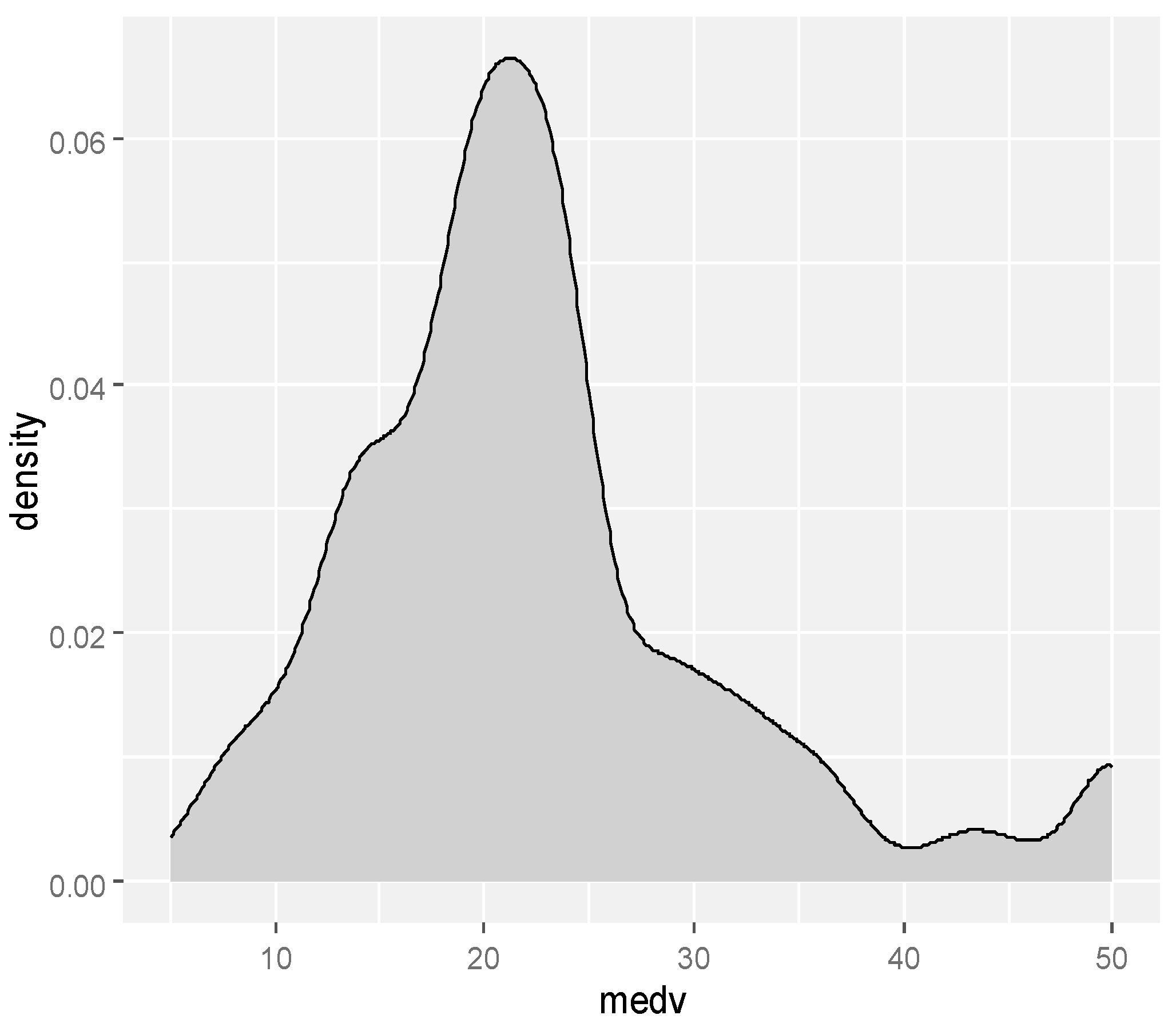
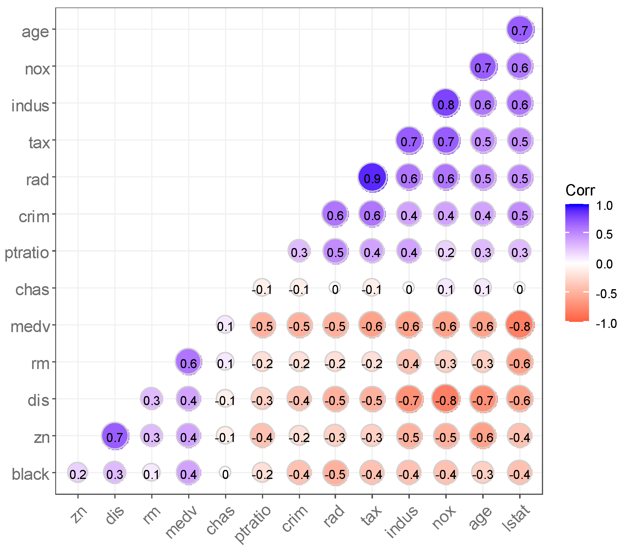
4.1. Data Analysis of House Prices in Boston Suburbs, USA

In this subsection, the proposed BLEL variable selection method is applied to the Boston housing prices dataset, which characterizes suburban housing prices in the U.S. This dataset comprises 506 observations and 14 variables, with no missing values. A detailed description of this dataset was available on 2 April 2025, via the following link: https://lib.stat.cmu.edu/datasets/boston.

We consider the following model:

$$Y=X^T\beta +\epsilon$$

where the covariate $X={\left(X_1,\dots ,X_{13}\right)}^T$ is the 13 variables that influence the house price data, and the dependent variable Y represents the median value of a home,

Table 5. Explanation of variables in the Boston suburbs housing price data set.

Variant	Name (of a Thing)	Variable Interpretation
Y	medv	Median value of owner-occupied dwellings (in USD 1000 increments)
X1	crim	Per capita urban crime rate
X2	zn	Percentage of residential lots on parcels over 25,000 square feet
X3	indus	Percentage of non-retail business space per town
X4	chas	1—along the river, 0—other
X5	nox	NOx concentration (ppm)
X6	rm	Average number of rooms per dwelling
X7	age	Proportion of owner-occupied housing built before 1940
X8	dis	Weighted average of distances to five Boston job centers
X9	rad	Radial road accessibility index
X10	tax	Full-value property tax rate on a per USD 10,000 basis
X11	ptratio	Teacher–student ratio in towns and cities
X12	black	Calculated from $1000{(B_k-0.63)}^2$, where $B_k$ is the percentage of urban blacks
X13	lstat	Percentage of population in the lower classes (%)

below shows the names of the variables in the house price dataset for the Boston suburbs and what they mean exactly:

As shown in Figure 1, the distribution of the response variable, house price (medv), exhibits right-skewness, deviating significantly from a normal distribution. This skewness indicates that the data contains a proportion of high-value outliers or follows a heavy-tailed distribution, necessitating the adoption of robust statistical methods—such as the composite quantile regression framework used in this study—to ensure the reliability of variable selection and parameter estimation. Unlike traditional least squares regression, which assumes normality, the proposed BLEL method is capable of capturing the asymmetric characteristics of house prices across multiple quantiles, thereby providing a more comprehensive understanding of the factors influencing housing prices in different segments of the distribution.

A box plot of the house price data (medv) is plotted below (Figure 2).

Outlier identification uses the Tukey box plot criterion: points outside Q3 + 1.5IQR or Q1 − 1.5IQR are considered statistical outliers. This standard is widely used in robust data analysis. The box plot of the house price data (MEDV) indicates that the data is concentrated between USD 17,000 and USD 25,000, though a substantial number of data points fall outside this range, suggesting the presence of potential outliers. A correlation analysis was performed on the variables in the Boston house price dataset, with results visualized in Figure 3. The analysis reveals that the response variable medv exhibits the highest absolute correlation coefficients with three variables:

Following these, variables with absolute correlation coefficients between 0.4 and 0.5 include indus (proportion of non-retail business acres, −0.40), tax (property tax rate, −0.46), nox (nitric oxide concentration, −0.42), and rad (highway accessibility index, 0.39). All other variables exhibit absolute correlation coefficients below 0.4, indicating weaker linear relationships with medv.

The comparison results using several methods such as LASSO, SCAD, BEL, and BLEL are shown in

Table 6. Results of variable estimation under different methods.

VARIAN	NAME	LASSO	SCAD	BEL	BLEL
X1	crim	−0.026	−0.108	0	0
X2	zn	0.001	0.046	0	0
X3	indus	0	0	0.15	0
X4	chas	2.084	2.718	0	0.474
X5	nox	−5.538	−17.38	−0.467	0
X6	rm	4.271	3.801	0	0.314
X7	age	0	0	−0.34	0
X8	dis	−0.467	−1.493	−0.82	0
X9	rad	0	0.299	0.665	0.401
X10	tax	0	−0.012	−0.427	−0.332
X11	ptratio	−0.811	−0.946	−0.297	−0.297
X12	black	0.006	0.009	0	−0.158
X13	lstat	−0.519	−0.523	−0.897	−0.829

below.

Based on the variable selection estimation results, the LASSO method selected 8 variables: crim, zn, chas, nox, rm, dis, ptratio, black, and lstat (note: the original mention of “8 variables” may include a typo, as listed names total 9); the SCAD method selected 10 variables: crim, zn, chas, nox, rm, dis, rad, tax, ptratio, black, and lstat (similarly, listed names total 11); the BEL method selected 9 variables: indus, nox, age, dis, rad, tax, ptratio, black, and lstat; and the BLEL method proposed in this study selected 7 variables: chas, rm, rad, tax, ptratio, black, and lstat.

The BLEL results indicate that variables with positive effects on housing prices include chas (Charles River proximity, binary), rm (average number of rooms), and rad (highway accessibility index), meaning homes near the river, larger dwellings, and better highway access are associated with higher prices. Conversely, variables with negative effects are tax (property tax rate), ptratio (pupil–teacher ratio), black (proximity to Black population), and lstat (lower-status population percentage), suggesting higher taxes, poorer educational resources, and higher socioeconomic disadvantage correlate with lower housing values. These findings align with both the correlation analysis and real-world expectations, validating the practical relevance of the BLEL method for variable selection.

To enhance data analysis accuracy, outliers were removed from the dataset. Specifically, 40 data points outside the box plot range were excluded, and the revised variable correlation coefficients are presented below:

Based on the box plot statistical criteria (Q1 − 1.5IQR, Q3 + 1.5IQR), 40 medv outliers were identified (Figure 2). After deletion, the variable correlation changed significantly (compare Figure 3 and Figure 4).

After outlier removal, the top seven variables in terms of absolute correlation coefficients with house price (medv) are lstat (lower-status population percentage), indus (non-retail business proportion), tax (property tax rate), nox (nitric oxide concentration), rm (average rooms per dwelling), age (older homes proportion), and rad (highway accessibility index), all with coefficients exceeding 0.5. This indicates stronger linear relationships after eliminating extreme values, emphasizing the influence of socioeconomic, environmental, and structural factors on housing prices.

The variable selection results from each method after outlier removal are as follows (

Table 7. Estimates of variables under different methods after removing outliers.

Variant	Name (of a Thing)	LASSO	SCAD	BEL	BLEL
X1	crim	−0.372	−0.84	0	0
X2	zn	0.117	0.85	0.178	0
X3	indus	−0.309	−0.025	−0.379	0
X4	chas	0.165	−0.253	0	0
X5	nox	−0.66	−1.398	−0.199	−0.487
X6	rm	1.175	1.085	0.068	0.231
X7	age	−0.21	−0.556	0	0
X8	dis	−0.056	−2.159	−0.29	−0.003
X9	rad	0	2.012	0.569	0.386
X10	tax	−0.35	−2.032	−0.511	−0.501
X11	ptratio	−1.278	1.441	−0.128	−0.443
X12	black	0.54	0.69	0	−0.111
X13	lstat	−2.671	−2.613	−0.47	−0.042

).

Based on the variable selection estimation results, the LASSO method retained 12 variables, excluding only rad (highway accessibility index), while the SCAD method selected all 13 explanatory variables without exclusion. The BEL method identified nine variables: zn, indus, nox, rm, dis, rad, tax, ptratio, and lstat, focusing on residential zoning, industrial proportion, environmental exposure, and socioeconomic factors. In contrast, the proposed BLEL method parsimoniously selected eight variables: nox, rm, dis, rad, tax, ptratio, and lstat, emphasizing key drivers with strong theoretical and empirical relevance.

The BLEL results reveal that rm (average number of rooms) and rad (highway accessibility index) exhibit positive associations with housing prices, aligning with economic intuition—larger homes and better transportation access typically command higher values. Conversely, nox (nitric oxide concentration), dis (distance to employment centers), tax (property tax rate), ptratio (pupil–teacher ratio), and lstat (lower-status population percentage) show negative effects, consistent with the hypothesis that pollution, longer commute distances, higher taxes, and socioeconomic disadvantage depress housing values. Notably, the variable Black (proximity to Black population), while present in earlier analyses, was excluded in this iteration, possibly due to reduced influence after outlier removal or collinearity with other socioeconomic indicators.

A critical strength of the BLEL method is its robustness: the core variables selected (e.g., rm, tax, lstat, and rad) remain stable before and after outlier removal, with only minor adjustments in peripheral variables. This consistency underscores BLEL’s ability to distinguish true signal from noise, even in datasets with heterogeneous data quality. The alignment between BLEL’s results, correlation analysis, and real-world housing dynamics—coupled with its resistance to data perturbations—validates its utility for robust variable selection in observational studies with complex data structures. These findings reinforce BLEL’s practical value for identifying invariant drivers of housing prices in the Boston area and beyond.

4.2. Analysis of Iowa Home Price Data

In this subsection, the proposed BLEL variable selection method is applied to the Ames, Iowa, housing prices dataset from the Kaggle platform (https://www.kaggle.com/c/house-prices-advanced-regression-techniques/data) to evaluate its performance in high-dimensional real-world data, accessed on 15 April 2025. The dataset comprises 1460 observations and 81 variables, presenting a complex high-dimensional scenario with inherent challenges such as missing values and skewed distributions.

(1)

Missing Value Handling:

• Variables with missing data exceeding 10% were removed to maintain data integrity.
• For numerical variables, missing values were imputed using the column mean.
• Categorical variables with missing values were filled with the mode (most frequent category).

(2)

Data Normalization:

Given the significant skewness in numerical data, all features were normalized to ensure scale consistency and improve model convergence. This step is critical for methods sensitive to feature scaling, such as those involving penalized regression.

The covariates consist of 35 numerical variables influencing house prices, with the dependent variable being “SalePrice”—the sale price of the house. As shown in Figure 5, the distribution of “SalePrice” deviates significantly from normality, exhibiting a pronounced right-skewness with a long tail toward higher values. This non-normal pattern indicates the presence of high-value outliers and heterogeneous data-generating processes, necessitating robust variable selection methods that are less sensitive to extreme values.

Variable selection for the factors affecting house prices was performed using LASSO, SCAD, BEL, and BLEL methods, with results compared in

Table 8. Comparison of selection variables between different selection methods.

Number of Individuals	Factor
LASSO	16	LotArea, OverallQual, OverallCond, YearBuilt, YearRemodAdd, BsmtFinSF1, TotalBsmtSF, X1stFlrSF, GrLivArea, BsmtFullBath, KitchenAbvGr, Fireplaces, GarageCars, GarageArea, WoodDeckSF, ScreenPorch
SCAD	27	LotArea, OverallQual, OverallCond, YearBuilt, YearRemodAdd, BsmtFinSF1, BsmtFinSF2, BsmtUnfSF, TotalBsmtSF, LowQualFinSF, GrLivArea, BsmtFullBath, FullBath, HalfBath, BedroomAbvGr, KitchenAbvGr, TotRmsAbvGrd, Fireplaces, GarageCars, GarageArea, WoodDeckSF, EnclosedPorch, X3SsnPorch, ScreenPorch, PoolArea, MiscVal, YrSold
BEL	24	MSSubClass, LotFrontage, LotArea, OverallQual, OverallCond, YearBuilt, YearRemodAdd, BsmtFinSF1, BsmtUnfSF, TotalBsmtSF, X1stFlrSF, GrLivArea, BsmtFullBath, FullBath, HalfBath, KitchenAbvGr, TotRmsAbvGrd, GarageCars, GarageArea, OpenPorchSF, X3SsnPorch, ScreenPorch, MiscVal
BEL LASSO	16	LotArea, OverallQual, OverallCond, YearBuilt, YearRemodAdd, BsmtFinSF1, TotalBsmtSF, X1stFlrSF, GrLivArea, BsmtHalfBath, BedroomAbvGr, TotRmsAbvGrd, Fireplaces, GarageCars, MiscVal, MoSold

.

In high-dimensional settings, the BLEL method stands out by selecting a relatively small number of variables while retaining critical features. This parsimony suggests that BLEL effectively distinguishes between valuable and redundant variables, filtering out noise and irrelevant predictors.

In summary, BLEL’s performance in selecting a sparse yet informative set of variables underscores its utility for high-dimensional real-world datasets like the Ames housing data, where balancing model complexity, interpretability, and robustness is essential. The results in Table 8 collectively demonstrate that BLEL offers a competitive alternative to traditional penalized methods, particularly in scenarios with skewed data and numerous predictors.

5. Conclusions

In this paper, focusing on the variable selection challenge within a composite quantile regression model in high-dimensional scenarios, we introduce the Bayesian LASSO empirical likelihood penalized variable selection method (BLEL), along with a hybrid sampling approach that integrates EM and M-H algorithms nested within Gibbs sampling. The proposed method is numerically compared against conventional LASSO, SCAD, and BEL methods for composite quantile regression, and Markov Chain Monte Carlo-based numerical simulations demonstrate its superiority. The method is further applied to analyze two housing price datasets, with results showing that the variables selected by BLEL exhibit the smallest discrepancy before and after removing outliers in the Boston housing price data, illustrating its robustness. In the variable selection for the Iowa housing price data, the BLEL method selects a relatively smaller number of variables from high-dimensional data, indicating its capability to efficiently filter out less important variables for improved data analysis. This method effectively screens out relatively unimportant variables, thereby providing practical assistance in reducing the impact of unknown data anomalies on the model.

References

1. Zou, H.; Yuan, M. Composite Quantile Regression and the Oracle Model Selection Theory. Ann. Stat. 2008, 36, 1108–1126. [Google Scholar] [CrossRef]
2. Huang, H.; Chen, Z. Bayesian composite quantile regression. J. Stat. Comput. Simul. 2015, 85, 3744–3754. [Google Scholar] [CrossRef]
3. Wang, J.F.; Fan, G.L.; Wen, L.M. Compound quantile regression estimation of regression functions under random missingness of censored indicators. Syst. Sci. Math. 2018, 38, 1347–1362. [Google Scholar]
4. Liu, H.; Yang, H.; Peng, C. Weighted composite quantile regression for single index model with missing covariates at random. Comput. Stat. 2019, 34, 1711–1747. [Google Scholar] [CrossRef]
5. Art, O. Empirical likelihood for linear models. Ann. Stat. 2007, 19, 1725–1747. [Google Scholar]
6. Art, O. Empirical likelihood ratio confidence regions. Ann. Stat. 2007, 18, 90–120. [Google Scholar]
7. Owen, B.A.; Cox, D.; Reid, N. Empirical Likelihood; CRC Press: Boca Raton, FL, USA, 2001. [Google Scholar]
8. Zhao, P.; Zhou, X.; Lin, L. Empirical likelihood for composite quantile regression modeling. J. Appl. Math. Comput. 2015, 48, 321–333. [Google Scholar] [CrossRef]
9. Lazar, A.N. Bayesian Empirical Likelihood. Biometrika 2003, 90, 319–326. [Google Scholar] [CrossRef]
10. Fang, K.; Mukerjee, R. Empirical-Type Likelihoods Allowing Posterior Credible Sets with Frequentist Validity: Higher-Order Asymptotics. Biometrika 2006, 93, 723–733. [Google Scholar] [CrossRef]
11. Yang, Y.; He, X. Bayesian empirical likelihood for quantile regression. Ann. Stat. 2012, 40, 1102–1131. [Google Scholar] [CrossRef]
12. Zhang, Y.; Tang, N. Bayesian empirical likelihood estimation of quantile structural equation models. J. Syst. Sci. Complex. 2017, 30, 122–138. [Google Scholar] [CrossRef]
13. Chaudhuri, S.; Mondal, D.; Yin, T. Hamiltonian Monte Carlo sampling in Bayesian empirical likelihood computation. J. R. Stat. Soc. Ser. B (Stat. Methodol.) 2017, 79, 293–320. [Google Scholar] [CrossRef]
14. Vexler, A.; Yu, J.; Lazar, N. Bayesian empirical likelihood methods for quantile comparisons. J. Korean Stat. Soc. 2017, 46, 518–538. [Google Scholar] [CrossRef] [PubMed]
15. Zhao, P.; Ghosh, M.; Rao, K.N.J.; Wu, C. Bayesian empirical likelihood inference with complex survey data. J. R. Stat. Soc. Ser. B (Stat. Methodol.) 2020, 82, 155–174. [Google Scholar] [CrossRef]
16. Dong, X.G.; Liu, X.R.; Wang, C.J. Bayesian empirical likelihood for accelerated failure time models under right-censored data. J. Math. Stat. Manag. 2020, 39, 838–844. [Google Scholar]
17. Bedoui, A.; Lazar, A.N. Bayesian empirical likelihood for ridge and lasso regressions. Comput. Stat. Data Anal. 2020, 145, 106917. [Google Scholar] [CrossRef]
18. Zhang, R.; Wang, D.H. Bayesian empirical likelihood inference for the generalized binomial AR(1) model. J. Korean Stat. Soc. 2022, 51, 977–1004. [Google Scholar] [CrossRef]
19. Sheng, C.L.; Ying, H.L. Bayesian empirical likelihood of quantile regression with missing observations. Metrika 2022, 86, 285–313. [Google Scholar] [CrossRef]
20. Tibshirani, R.J. Regression Shrinkage and Selection via the LASSO. J. R. Stat. Soc. Ser. B 1996, 58, 267–288. [Google Scholar] [CrossRef]
21. Fan, J.; Li, R. Variable Selection via Non-concave Penalized Likelihood and Its Oracle Properties. J. Am. Stat. Assoc. 2001, 96, 1348–1360. [Google Scholar] [CrossRef]
22. Zou, H. The Adaptive LASSO and Its Oracle Properties. J. Am. Stat. Assoc. 2006, 101, 1418–1429. [Google Scholar] [CrossRef]
23. Zou, H.; Hastie, T. Regularization and Variable Selection via the Elastic Net. J. R. Stat. Soc. Ser. B 2005, 67, 301–320. [Google Scholar] [CrossRef]
24. Mitchell, T.J.; Beauchamp, J.J. Bayesian variable selection in linear regression. J. Am. Stat. Assoc. 1988, 83, 1023–1032. [Google Scholar] [CrossRef]
25. Nardi, Y.; Rinaldo, A. Autoregressive process modeling via the lasso procedure. J. Multivar. Anal. 2011, 102, 528–549. [Google Scholar] [CrossRef]
26. Schmidt, D.F.; Makalic, E. Estimation of stationary autoregressive models with the Bayesian lasso. J. Time Ser. Anal. 2013, 34, 517–531. [Google Scholar] [CrossRef]
27. Kwon, S.; Lee, S.; Na, O. Tuning parameter selection for the adaptive Lasso in the autoregressive model. J. Korean Stat. Soc. 2017, 46, 285–297. [Google Scholar] [CrossRef]
28. Ishwaran, H.; Rao, J.S. Spike and Slab Variable Selection: Frequentist and Bayesian Strategies. Ann. Stat. 2005, 33, 730–773. [Google Scholar] [CrossRef]
29. Malsiner-Walli, G.; Wagner, H. Comparing spike and slab priors for Bayesian variable selection. Austrian J. Stat. 2011, 40, 241–264. [Google Scholar] [CrossRef]
30. Narisetty, N.N.; He, X. Bayesian variable selection with shrinking and diffusing priors. Ann. Stat. 2014, 42, 789–817. [Google Scholar] [CrossRef]
31. Luo, Y.X.; Li, H.F. Research on random effects quantile regression model based on double adaptive Lasso penalty. J. Quant. Econ. Tech. Econ. Res. 2017, 34, 136–148. [Google Scholar]
32. Luo, Y.X.; Li, H.F. Simulation study on dimension reduction algorithm for longitudinal data quantile regression model. Stat. Decis. 2018, 34, 5–9. [Google Scholar]
33. Xu, Y.J.; Luo, Y.X. Principal component Lasso dimension reduction algorithm and simulation based on variable clustering. Stat. Decis. 2021, 37, 31–36. [Google Scholar]
34. George, E.I.; Mcculloch, R.E. Variable selection via Gibbs sampling. J. Am. Stat. Assoc. 1993, 88, 881–889. [Google Scholar] [CrossRef]
35. Nascimento, M.G.L.; Gonçalves, K.C.M. Bayesian variable selection in quantile regression with random effects: An application to Municipal Human Development Index. J. Appl. Stat. 2022, 49, 3436–3450. [Google Scholar] [CrossRef] [PubMed]
36. Priya, K.; Damitri, K.; Kiranmoy, D.A. Bayesian variable selection approach to longitudinal quantile regression. Stat. Methods Appl. 2022, 32, 149–168. [Google Scholar] [CrossRef]
37. Taddy, A.M.; Kottas, A. A Bayesian nonparametric approach to inference for quantile regression. J. Bus. Econ. Stat. Econ. Stat. 2010, 28, 357–369. [Google Scholar] [CrossRef]
38. Androulakis, E.; Koukouvinos, C.; Vonta, F. Estimation and variable selection via frailty models with penalized likelihood. Stat. Med. 2012, 31, 2223–2239. [Google Scholar] [CrossRef] [PubMed]
39. Li, C.J.; Zhao, H.M.; Dong, X.G. Bayesian empirical likelihood and variable selection for censored linear model with applications to acute myelogenous leukemia data. Int. J. Biomath. 2019, 12, 799–813. [Google Scholar] [CrossRef]
40. Xi, R.; Li, Y.; Hu, Y. Bayesian quantile regression based on the empirical likelihood with spike and slab priors. Bayesian Anal. 2016, 11, 821–855. [Google Scholar] [CrossRef]
41. Li, C.J. Bayesian Empirical Likelihood Statistical Inference for Regression Models Under Censored Data. Ph.D. Thesis, Jilin University, Changchun, China, 2019. [Google Scholar]
42. Tang, Y.C.; Leng, C. Penalized high-dimensional empirical likelihood. Biometrika 2010, 97, 905–919. [Google Scholar] [CrossRef]
43. Lahiri, N.S.; Mukhopadhyay, S. A penalized empirical likelihood method in higah dimensions. Ann. Stat. 2012, 40, 2511–2540. [Google Scholar] [CrossRef]
44. Ren, Y.; Zhang, X. Variable selection using penalized empirical likelihood. Sci. China Math. 2011, 54, 1829–1845. [Google Scholar] [CrossRef]
45. Bayati, M.; Ghoreishi, K.S.; Wu, J. Bayesian analysis of restricted penalized empirical likelihood. Comput. Stat. 2021, 36, 1321–1339. [Google Scholar] [CrossRef]
46. Moon, C.; Bedoui, A. Bayesian elastic net based on empirical likelihood. J. Stat. Comput. Simul. 2023, 93, 1669–1693. [Google Scholar] [CrossRef]
47. Liya, F.; Shuwen, H.; Jiaqi, L. Robust penalized empirical likelihood in high dimensional longitudinal data analysis. J. Stat. Plan. Inference 2024, 228, 11–22. [Google Scholar]
48. Park, T.; Casella, G. The Bayesian LASSO. J. Am. Stat. Assoc. 2008, 103, 681–686. [Google Scholar] [CrossRef]
49. Gilks, W.; Richardson, S.; Spiegelhalter, D. Markov Chain Monte Carlo in Practice; Chapman and Hall: New York, NY, USA, 1996. [Google Scholar]
Figure 1. Distribution of dependent variable (medv).
Mathematics 13 02287 g001
Figure 2. Box plot of medv with outliers identified by Tukey’s method (points beyond 1.5 × IQR).
Mathematics 13 02287 g002
Figure 3. Correlation analysis of variables for house price data.
Mathematics 13 02287 g003
Figure 4. Correlation analysis of house price data variables after removal of outliers.
Mathematics 13 02287 g004
Figure 5. Distribution of dependent variable (SalePrice).
Mathematics 13 02287 g005