1. Introduction
Multi-criteria decision making (MCDM) is a key branch of decision theory. It can be divided into two categories based on the nature of the solution space as follows: continuous and discrete. Continuous MCDM is addressed using multi-objective decision making (MODM), while discrete MCDM is tackled through multi-attribute decision making (MADM). This paper focuses exclusively on the latter. In the literature, the term MCDM often refers to discrete MCDM (i.e., MADM), and we will use this terminology throughout. Over recent decades, numerous MADM methods have been proposed, including AHP [
1,
2,
3], ANP [
4], TOPSIS [
5,
6,
7,
8,
9], ELECTRE [
10,
11,
12], VIKOR [
13,
14], and PROMETHEE [
15,
16,
17]. Simultaneously, as the volume of information and influencing factors in decision-making processes has increased, it has become evident that scientific decision making cannot be achieved by an individual alone. This has led to the development of group decision making (GDM), which harnesses collective wisdom for optimal decisions [
18,
19,
20]. Today, multi-attribute group decision making (MAGDM) is widely applied across various fields, including engineering, technology, economics, management, and the military. This paper specifically examines MAGDM.
MAGDM typically involves several key elements as follows:
Multiple Alternatives: Before making a decision, the decision maker (DM) must evaluate various alternatives.
Multiple Evaluation Criteria (Attributes): Decision makers must identify relevant factors that may affect the decision. These factors may be independent or interrelated, and it is necessary to define and measure the applicable criteria (attributes) before scoring by experts.
Allocation of Criteria Weights: Different criteria have varying levels of influence on the decision, necessitating distinct weights for each. Typically, the allocation of criteria weights is normalized [
21,
22].
Allocation of Expert Weights: Since GDM involves a group rather than a single individual, the allocation of expert weights is essential. The influence of each DM on the final decision varies, which requires assigning appropriate weights to each expert.
The determination of weights plays a critical role in MAGDM, making the problem of assigning reasonable weights to both experts and criteria a topic of significant interest. The weights of criteria reflect their relative importance and are crucial to the accuracy of decision results. Currently, methods for determining criteria weights tend to be simple, feasible, and practical. However, expert weight calculation is often complex, and its objectivity and accuracy are sometimes questionable, leaving the issue unresolved. Without any prior knowledge of the experts, a common assumption is that all experts are equally weighted. However, factors such as popularity, title, education, field relevance, and years of experience can all influence an expert’s contribution to the final judgment. Thus, different experts should be assigned distinct weights.
The variation in expert weights in GDM significantly alters the final decision, making the determination of expert weights a central concern in academic research. Generally, expert weight determination methods fall into three categories: subjective weighting, objective weighting, and a combination of both.
Subjective Weighting: In this method, the weights of each expert are predetermined or established through interactions between experts [
23,
24,
25]. While this method is independent of the evaluation results, it requires a high degree of expertise and familiarity among the experts. However, it remains highly subjective and uncertain.
Objective Weighting: This method determines expert weights based on a judgment matrix constructed from expert evaluations of the information. The weights change as evaluation results evolve [
26]. For example, [
27] addresses the supplier selection problem by integrating expert weights using hesitancy and similarity in evaluations, applying the TOPSIS method to rank suppliers. Similarly, [
28] introduces fault detection into FMEA and uses fuzzy theory and D-S evidence theory to allocate expert weights more reasonably, addressing the subjective limitations of traditional FMEA.
Combined Subjective and Objective Weighting: Some studies combine both subjective and objective perspectives. For instance, [
29] integrates subjective and objective weight matrices using the minimum entropy criterion, accounting for differing judgments by all DMs. Similarly, ref. [
30] combines expert weight coefficients and entropy weighting through fuzzy hierarchical analysis (FAHP), integrating both subjective and objective weights based on criteria characteristics to determine final weights.
This paper proposes an optimization model for determining expert weights in MAGDM, drawing on evaluation data from all experts. The model’s theoretical foundations are rigorously analyzed, and numerical experiments validate the conclusions. In comparison to existing expert-weighting methods, the proposed optimization model delivers several key advantages and overcomes their inherent limitations. Unlike purely subjective approaches, it requires no self-assessment or pairwise comparisons, thereby eliminating arbitrary bias and uncertainty. Unlike conventional objective methods—such as entropy weighting, which derive weights solely from score dispersion—our model directly minimizes the aggregate deviation between individual evaluations and the group consensus point, ensuring maximal coherence in the final decision. Together with its proven existence, uniqueness, and “perfect rationality,” as well as an efficient nonlinear-equation–based solution algorithm, these features demonstrate the necessity and superiority of our framework for robust, transparent, and computationally tractable expert-weight assignment in MAGDM [
31,
32,
33]. We hope to find a more objective method for determining expert weights, one that has better properties than other methods. To achieve this, we attempt to use optimization-related theories for derivation and verification.
The contributions of this paper are as follows:
An optimization model is developed to minimize the discrepancies between individual expert evaluations and the overall group evaluation.
The existence and uniqueness of the model’s solution are theoretically proven, assuming full-rank conditions for the overall matrix column, and verified through numerical experiments.
The expert weights derived from the optimization model exhibit “perfect rationality”, meaning they are inversely proportional to the distance from the “overall consistent scoring point”. This property is demonstrated through theoretical derivations.
A simplified algorithm for solving expert weights is proposed, leveraging the “perfect rationality” principle and transforming the model into a system of nonlinear equations.
The structure of the paper is as follows:
Section 2 introduces the problem to be solved.
Section 3 presents the optimization model for determining expert weights based on overall consistency in expert evaluations.
Section 4 analyzes the model, proves the uniqueness of the solution, demonstrates “perfect rationality”, and outlines a simplified solution algorithm.
Section 5 presents numerical experiments that validate the proposed methods.
2. Problem Description
Determining expert weights objectively is a central issue in current academic research. Existing objective weighting methods can be grouped into three main approaches as follows: (1) using experts to determine the proportion of the judgment matrix scale to assign expert weights, assessing the importance, truthfulness, and credibility of the information provided by each expert, and then determining their weight [
26,
34]; (2) employing the eigenvectors of the judgment matrix to evaluate the contribution of the information provided by each expert in order to calculate their weight [
35,
36]; and (3) using the consistency ratio of the judgment matrix to assess the quality of the judgmental information provided by the experts and determine their corresponding weights [
37,
38,
39].
In response to this, this paper develops an optimization model to determine expert weights based on the evaluation results of all experts involved in decision making. The objective is to minimize the sum of differences between individual evaluations and the overall consistent evaluation. For multi-attribute group decision making (MAGDM) involving multiple alternatives, the following sets are commonly used:
The set of criteria (attributes):
The set of criteria (attributes): , where n represents the number of criteria associated with the alternatives being evaluated.
The set of alternatives: , where s represents the number of alternatives under evaluation.
The set of experts (decision makers): , where m represents the number of experts involved in the evaluation.
In practice, multiple experts are often tasked with scoring alternatives from different perspectives (i.e., based on various criteria) and making decisions based on these scores. Given the variability in their qualifications, experience, and expertise, not all experts hold equal authority in the decision-making process. This highlights the necessity of developing a robust method to determine expert weights. It can be argued that the evaluations of experts with more experience, specialized knowledge, and seniority carry more weight in decision making. In other words, experts whose evaluations are more authoritative should be assigned higher weights. In this paper, expert importance is measured by the difference between individual evaluations and the comprehensive group evaluation. The smaller this difference, the closer the expert’s evaluation is to the group’s consistent evaluation, indicating a higher level of agreement among experts. Based on this concept, we propose an optimization model for determining expert weights [
40].
3. The Optimization Models for Expert Weight Determination
Assume that expert
assigns a score of
to the
k-th criteria
of alternative
. The vector of scores provided by expert
for alternative
can be represented as
, where
,
, and
. For alternative
, the overall score is given by the matrix
, as follows:
For matrix , the k-th row represents the evaluation scores from all experts for the k-th criteria of alternative , and the j-th column represents the evaluation scores from expert for all criteria of alternative . The expert weight vector is denoted as , which needs to be determined.
The core idea of this paper is to develop an optimization model that uses the evaluation results of experts on multiple attributes of each alternative to objectively determine their respective weights. It is important to note that the term “experts” here is generalized as follows: all decision makers (DMs) involved in the process are considered “experts” in this context. In practical group decision making (GDM), decision makers often include individuals with varied expertise, and multiple groups may contribute their suggestions.
For alternative
, there exists an ideal scoring result, which is obtained by linearly weighting the evaluation results from all
m experts. This result reflects the consensus of the expert group and is referred to as the “consistent scoring point” of alternative
, denoted as
. This consistent scoring point is an
n-dimensional vector expressed as follows:
The distance between an individual expert’s scoring vector
and the consistent scoring point
is given by
, which measures the degree to which expert
’s evaluation aligns with the expert group’s evaluation. A larger value of
indicates a greater difference between the expert’s evaluation and the group’s consensus, suggesting lower authority for expert
in the group decision-making process. As a result, experts with larger
values should be assigned lower weights in order to improve the consistency of group decision making. The total discrepancy for alternative
, denoted as
, is the sum of all individual distances expressed as follows:
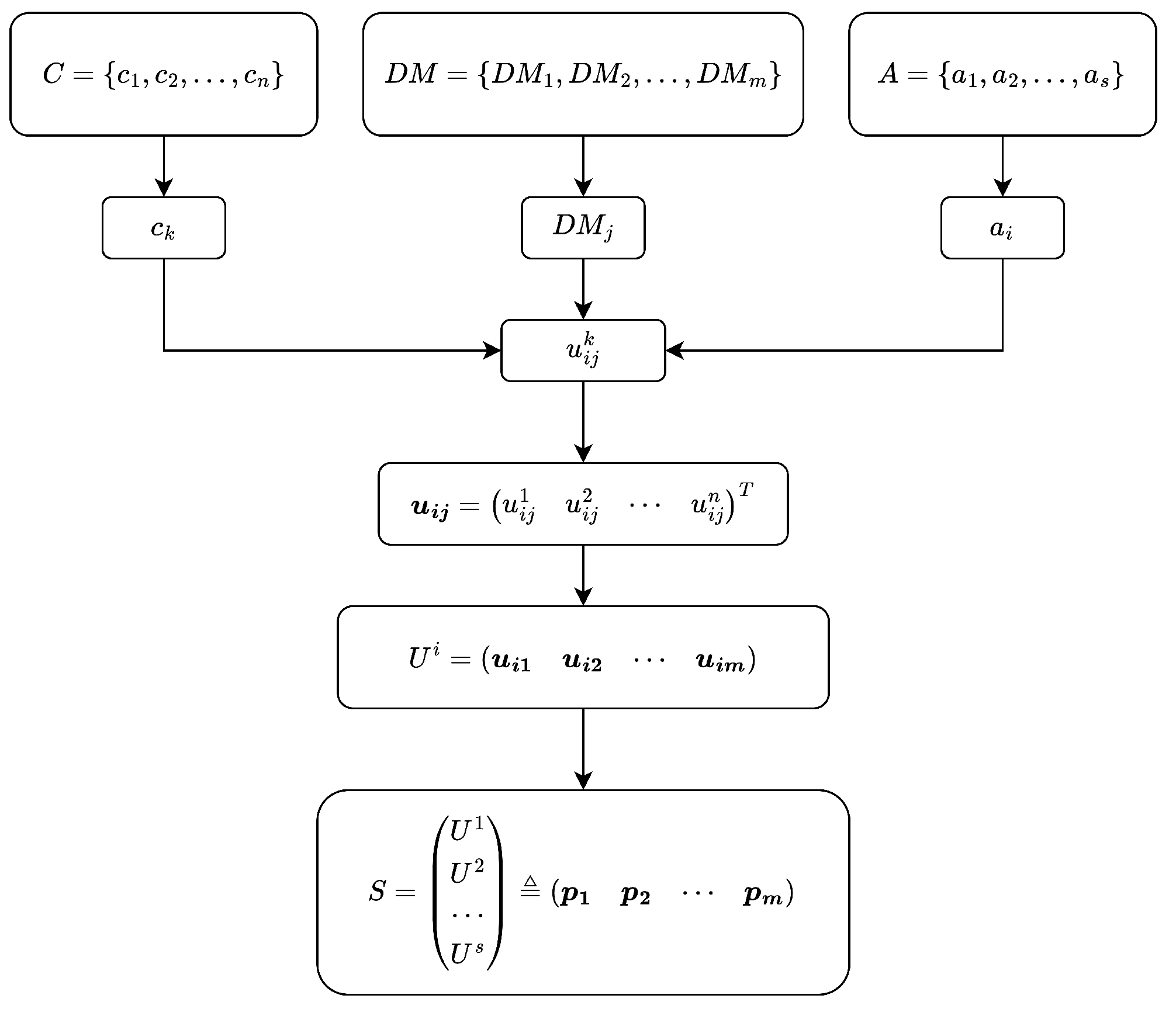
To make full use of the evaluation information from all experts for each alternative, the data corresponding to all alternatives can be integrated into a chunked matrix. This matrix allows for the determination of an overall “consistent scoring point”, which serves as the basis for constructing an integrated optimization model to derive a unique set of expert weights. Let
S denote this integrated matrix as follows (
Figure 1):
Here, each column vector
represents the scores assigned by expert
to the criteria of all alternatives. The “overall consistent scoring point”
is the
-dimensional column vector consisting of the consistent scoring points
for all alternatives, and is given by:
The consensus evaluation of decision makers under different options can only reflect the overall opinion under the alternative. However, if we want to rank or select the best among these options, we need to integrate these consensus evaluation results to unify the final decision results. We call it “overall consistent scoring point”, which represents the consensus evaluation conclusion of the decision group during the entire decision-making process.
The distance between the evaluation scores of expert
and the overall consistent scoring point
is given by
. Based on this, the optimization problem is formulated as follows:
Here, represents the objective function, which aims to minimize the sum of the distances between the individual expert evaluations and the overall consistent scoring point, thereby determining the expert weights that maximize the consistency of the group decision. Minimizing this objective ensures that the final expert weights reflect the most consistent evaluations.
Remark 1. The model adopts the sum of distances rather than the sum of squared distances as its objective function—in other words, it uses the norm instead of the norm. When the objective is instead formulated with the latter, the optimization problem admits a unique local optimum, which occurs precisely at equal weighting. This result can be established by a straightforward proof. In other words, regardless of how large or small the discrepancies among decision--makers’ evaluations may be, an -norm-based model will always assign equal weights to all experts. Consequently, it fails to capture the influence of inter-expert consistency on the resulting weights and thus cannot serve its intended purpose of deriving meaningful expert weights.
Remark 2. The objective of the model is to determine expert weights based on their evaluations, with the aim of achieving consistency across the evaluations of multiple decision makers, where greater consistency is preferred. To this end, we have developed the optimization model described above, where the objective function represents the sum of the discrepancies between each decision maker’s evaluation and the overall consistency evaluation. By minimizing this objective function, we obtain the optimal expert weights.
On the one hand, individual evaluations should be consistent. If the differences between expert evaluations are large, the final comprehensive evaluation may be biased. Thus, we aim to minimize the distance between each expert’s evaluation and the “overall consistent scoring point” to increase the consistency of group decision making. Experts whose evaluations are closer to the overall evaluation should receive higher weights, as their evaluations are considered more informative and authoritative. On the other hand, since all experts are assumed to be specialized, it is important that the deviation between the integrated evaluation and each expert’s evaluation is not excessively large. The expert weights obtained through this optimization model ensure the highest consistency between the integrated decision and the individual expert evaluations, while also maintaining the professionalism and credibility of the final evaluation.
In contrast to existing methods, which often rely on judgment matrices that require experts to subjectively measure the importance of evaluation criteria, this approach directly uses expert evaluations, making it more feasible and easier to implement. This optimization model is more aligned with practical decision-making scenarios and thus has both theoretical and practical value.
Remark 3. Building on the idea, the magnitude of the expert weights should be positively correlated with the consistency between the decision maker’s evaluation and the overall evaluation. In other words, the larger the discrepancy between the expert’s evaluation and the overall evaluation, the smaller the weight assigned to that expert, indicating a negative correlation. Moreover, in subsequent sections, we will theoretically establish this negative correlation and even demonstrate a strict inverse relationship, thereby confirming the fundamental purpose of our model.
The method of solving expert weights can be organized into the following algorithmic form (Algorithm 1):
| Algorithm 1 Algorithm for solving expert weights |
- 1:
Each decision maker evaluates each criteria under each plan to obtain - 2:
Obtain the evaluation matrix of the decision maker under each alternative plan - 3:
Concatenate the matrices to obtain the integrated matrix S, thereby obtaining the evaluation column vector of each decision maker - 4:
Calculate the expression of “overall consistent scoring point” - 5:
Use the SLSQP algorithm to solve the optimization model ( 6) - 6:
return Expert weight vector
|
SLSQP is a member of the sequential quadratic programming (SQP) family. Each iteration typically involves constructing a quadratic subproblem, solving the QP, performing a line search or trust region step, and updating the Hessian approximation, often using BFGS. The dominant computational cost of the SLSQP method arises from solving the quadratic programming (QP) subproblem in each iteration, primarily due to matrix decomposition. The per-iteration time complexity is , leading to a total time complexity of , where K is the number of iterations. The space complexity is .
4. Analysis of the Mathematical Properties of the Model
In this section, we introduce three key features of the model. First, based on the theory of partially convex optimization, we prove the uniqueness of the model’s solution. Second, by deriving the Karush–Kuhn–Tucker (KKT) conditions for the optimization problem, we demonstrate that the expert weights are inversely proportional to the distances from the “overall consistent scoring point”, thereby confirming the “perfect rationality” of the model. Finally, leveraging this inverse relationship, we reformulate the solution problem into a system of nonlinear equations, which improves the computational efficiency.
4.1. Existence and Uniqueness of the Solution
We prove the existence and uniqueness of the solution to the optimization problem (
6), based on the theory of partially convex optimization.
Definition 1 (Convex Function [
41])
. Let be a non-empty convex set, and let f be a function defined on S. The function f is called convex on S if, for any , , , the following inequality holds: Additionally, f is called strictly convex on S if the strict inequality holds when . Definition 2 (Convex Optimization [
41])
. The constrained problem is called a convex optimization problem if both the objective function and the constraint functions are convex and the constraint functions are linear. Lemma 1 (Existence of Convex Optimization Solutions [
42])
. Consider the convex optimization problem (8), and let D be the feasible region of the problem, defined as follows: If D is a non-empty compact set and f is continuous on D, then an optimal solution exists. Lemma 2 (Uniqueness of Convex Optimization Solutions [
43])
. Consider the convex optimization problem (8), and let D be the feasible region of the problem. Then,- 1.
If the problem has a local optimal solution , then is also the global optimal solution;
- 2.
The set of global optimal solutions is convex;
- 3.
If the problem has a local optimal solution and is strictly convex on D, then is the unique global optimal solution.
Theorem 1. The objective function is strictly convex when the columns of the matrix S are of full rank.
Proof. We define the objective function as follows:
. Let
and
be two distinct weight vectors that satisfy the constraints, with
and
. We then consider the following:
Next, we express the combination of
and
as follows:
Let and be defined as follows: and . Now, define the function as follows: .
This yields the following:
Thus, we obtain the following:
.
Since
is positive and the L2-norm of any vector is non-negative, both
and
must be non-negative. Squaring both terms and taking the difference yields the following:
Expanding both terms yields the following:
This simplifies to the following:
Since
, it follows that
is a positive real number. By the Cauchy–Schwarz inequality, the following can be derived:
where the equality holds if and only if
and
are linearly related. From this, we deduce the following:
Thus, it follows that holds. Since both and are non-negative, we conclude that , which implies , and therefore, the objective function is convex.
Since
, for the inequality in (
12) to hold strictly,
cannot hold simultaneously for all
. To prove this, we proceed by contradiction. Suppose that
for all
j. Then, for each
j, the vector
must be linearly related to the vector
. This implies that for some scalar
, we have the following:
Since the matrix columns are assumed to be of full rank, meaning that the column vectors are linearly independent, the coefficients of the vector
must be zero. This leads to the following system of equations:
For
, we obtain the following:
Additionally, for
, we have the following:
From the system in (
20), we deduce that
and
. Substituting this into (
21) yields
, which implies that:
, and consequently,
for all
, which contradicts the assumption that
. Therefore, the assumption that
for all
j is false.
Thus,
cannot hold simultaneously, implying that the inequality in (
12) is strict. Consequently, we conclude that the objective function
is strictly convex when the matrix columns are of full rank. □
Theorem 2. If the columns of S are of full rank, the solution to the optimization problem (6) exists and is unique. Proof. To facilitate analysis, we rewrite (
6) in the standard form as follows:
Here, the functions
and
are convex, and the equality constraint
is linear. Since
is convex, by Definition 2, (
6) is a convex optimization problem. Therefore, by Lemma 1, we conclude that a local optimal solution exists.
From Theorem 1, we know that when the matrix S has full rank, is not only convex but also strictly convex. Thus, by Lemma 2, the local optimal solution is also the global optimal solution. Therefore, the solution exists and is unique, completing the proof. □
Remark 4. In many real-world problems, additional requirements or constraints often arise. To accommodate these conditions, supplementary constraints can be incorporated into the base model. For instance, in practical applications, if we know that expert a is more qualified than expert b for evaluating the alternative, we can impose a new constraint in Equation (6) to ensure that the optimization problem respects these requirements. The addition of such constraints is flexible, provided they ensure the convexity of (6), thus guaranteeing the uniqueness of the solution and the appropriate expert weights for the decision model. The matrix S has rows and m columns, where n is the number of criteria and s is the number of alternatives. In practice, we aim to increase the number of decision makers (DMs) while maximizing the number of alternatives and evaluation criteria. This typically results in a matrix S with more rows than columns, increasing the likelihood that the columns of S are of full rank.
4.2. The “Perfect Rationality” of Model
When constructing the model, we aim to ensure that the smaller the distance between an expert’s evaluation and the “overall consistent scoring point”, the greater the weight assigned to the expert. In other words, expert weights are negatively correlated with the distance, and the ideal situation is that the expert’s weight is strictly inversely proportional to the corresponding distance. Based on this negative correlation between weights and distances, we propose the following definition:
Definition 3 (Deviation)
. Let the product of the weight of expert and the corresponding distance be denoted by . The deviation of the weight-distance product for expert is defined as , where is the average of the weight-distance products of all experts, and m is the total number of experts involved in the decision-making process. Thus, the average relative deviation is defined as the “deviation” of the model when the weights are , as follows: Definition 4 (Perfect Rationality). The model is considered to exhibit “perfect rationality” under the expert weights when the “deviation” is zero.
Remark 5. Based on the two definitions above, we can conclude that the model has “perfect rationality” if and only if the expert weights are strictly inversely related to the distances corresponding to the “overall consistent scoring point”.It is evident that implies , which leads to . This in turn suggests that , indicating that the weights are inversely proportional to the distance. The converse is also true.
Lemma 3 (Sufficient and Necessary Conditions for Optimality in Convex Optimization [
41])
. If the objective function and the constraint functions and are both differentiable and the optimization problem satisfies Slater’s condition, then the Karush–Kuhn–Tucker (KKT) conditions provide a sufficient and necessary condition for optimality. Slater’s condition ensures that the optimal duality gap is zero and that the dual optimum is attained. Thus, is optimal if and only if both and satisfy the KKT conditions. The optimal expert weights obtained from the optimization model (
6) are denoted as
, where
is the optimal weight of expert
, and
is the distance from the evaluation point of expert
to the “overall consistent scoring point”
. At this point,
.
Theorem 3. The optimal expert weights obtained from the optimization model (6) exhibit “perfect rationality”. Proof. The standard form of the optimization model (
6) is written as (
22), and by the definition of the KKT conditions [
41], the KKT conditions for this optimization model are expressed as follows:
From the last six equations, we conclude that
, so the first equation simplifies to the following:
The partial derivative of
is as follows:
Thus, we can rewrite the gradient of
as follows:
Substituting this into (
25), we get the following:
The above equation holds for any
k. Thus, for
, we have the following:
Assuming
, it follows that
, and thus, the following holds:
.
Since
and the evaluation vectors of each expert are linearly independent, the coefficients corresponding to the evaluation vectors of the experts in the above sum must be zero. For expert
, whose evaluation vector is
, the corresponding equation is as follows:
Substituting
, we rewrite Equation (
30) as follows:
which simplifies to the following:
Equation (
32) holds for any
j, and the right-hand side is constant when the optimal weights are obtained. Thus, we conclude that the product of the optimal weights and their corresponding distances to the “overall consistent scoring point” is constant. This implies that the optimal weights are strictly inversely proportional to the distances at this point, so
and
. Therefore, the model exhibits “perfect rationality”. □
4.3. Solving Algorithms Based on “Perfect Rationality”
The expert weights can be determined by solving the optimization problem to obtain its optimal solution. From Theorem 3, we know that when the optimization problem reaches its optimal solution, the expert weights are inversely proportional to the distances. Since it is sufficient for the optimization problem to reach the optimal solution and for the solution to satisfy the Karush–Kuhn–Tucker (KKT) conditions, we can transform the optimization model. The transformed solution is equivalent to the original optimization model’s solution. Based on this approach, we propose the following system of nonlinear equations:
where
. The optimal weights,
, are the solutions to this system of equations.
Since calculating
in the above system is computationally complex, we can further transform the system to improve efficiency. The equivalent system of nonlinear equations is as follows:
By solving this system of nonlinear equations, we can obtain the same expert weights as those obtained by solving the optimization model. This result will be further verified through numerical experiments.
5. Numerical Experiment
To validate the two models discussed above, we generated multiple sets of data and performed numerical experiments to observe regular patterns in the results. In the following section, we introduce and analyze the proposed models using the problem represented by the dataset in
Table 1 as an example.
We select seven experts
from six evaluation criteria
and five alternatives
for scoring. Based on these data, decisions are made. The evaluation matrix
for each alternative is constructed, and the data presented in
Table 1 are used to assemble the matrix
S. From this, the evaluation vector
for each expert is derived. The weight vector for the experts is represented as
. All numerical experiments were performed on a laptop equipped with an Intel(R) Core(TM) i5-8265U CPU @ 1.60 GHz, 1800 Mhz, 4 cores, and 8 logical processors, the operating system was Windows 11, and the calculation process used MATLAB R2019a. In solving the optimization problem, the initial weight vector is set as the mean weight. The optimal expert weights for models (
6) and (
34) are then computed using the SLSQP and trust region methods [
41], respectively. In solving the nonlinear equation system, we set the initial weight to the equal weight and the threshold to 1 × 10
−12. After 3 iterations using Matlab, we can obtain the expert weight. The results are presented in
Table 2 and
Table 3.
First, from the results in
Table 2, it is evident that the optimization model yields the optimal expert weights with a “deviation” of only
. At this point, the distance between the expert weights and the corresponding “overall consistent scoring point” is approximately 66.5948. This suggests an inverse relationship between the weights and the distance, implying that the model, with its optimal expert weights, demonstrates “perfect rationality”. The distance between the optimal expert weights and their corresponding distances is visualized in
Figure 2. Additionally, when comparing the results under the optimal weights with those obtained from equally distributed expert weights, the objective function value and “deviation” are smaller under the optimal weights. This indicates that the optimization model’s determination of expert weights is rational and justified.
Secondly, the results of solving expert weights using the optimization model and the nonlinear system of equations model are presented in
Table 2 and
Table 3, respectively. The optimal expert weights obtained by both models are identical, given by
. From the results in both tables, it is clear that the optimization model requires 10 iterations to solve for the expert weights, while the nonlinear system of equations model requires only 3 iterations to obtain the ideal weights. This demonstrates that transforming the problem into a system of nonlinear equations reduces the number of iterations and improves computational efficiency, highlighting the feasibility of using the nonlinear system to solve for expert weights as the solution approach for the targeted model.
To assess the effectiveness of our proposed weighting model, we applied the entropy weight method (EWM) to the same dataset (
Table 1) and compared its expert weights with those obtained from our optimization model (
Table 2 and
Table 3). We also computed the deviation values under the entropy-based weights to facilitate a direct comparison.
The entropy method assigns higher weights to experts whose evaluation scores exhibit greater dispersion (and therefore more information). This principle aligns with the rationale of our optimization model, making it a suitable benchmark. Specifically, each column of the evaluation matrix is normalized to
, and then entropy and dispersion are calculated; the normalized dispersion scores yield the entropy-based weights. We then computed the corresponding deviation metric for these weights and present the results in
Table 4.
As shown, although the two methods produce different weight magnitudes, the overall ranking of decision makers remains largely unchanged. Crucially, the deviation values under our optimization model are substantially lower than those from the entropy method. This demonstrates that the expert weights derived from our model achieve a higher level of consensus in the decision-making process.
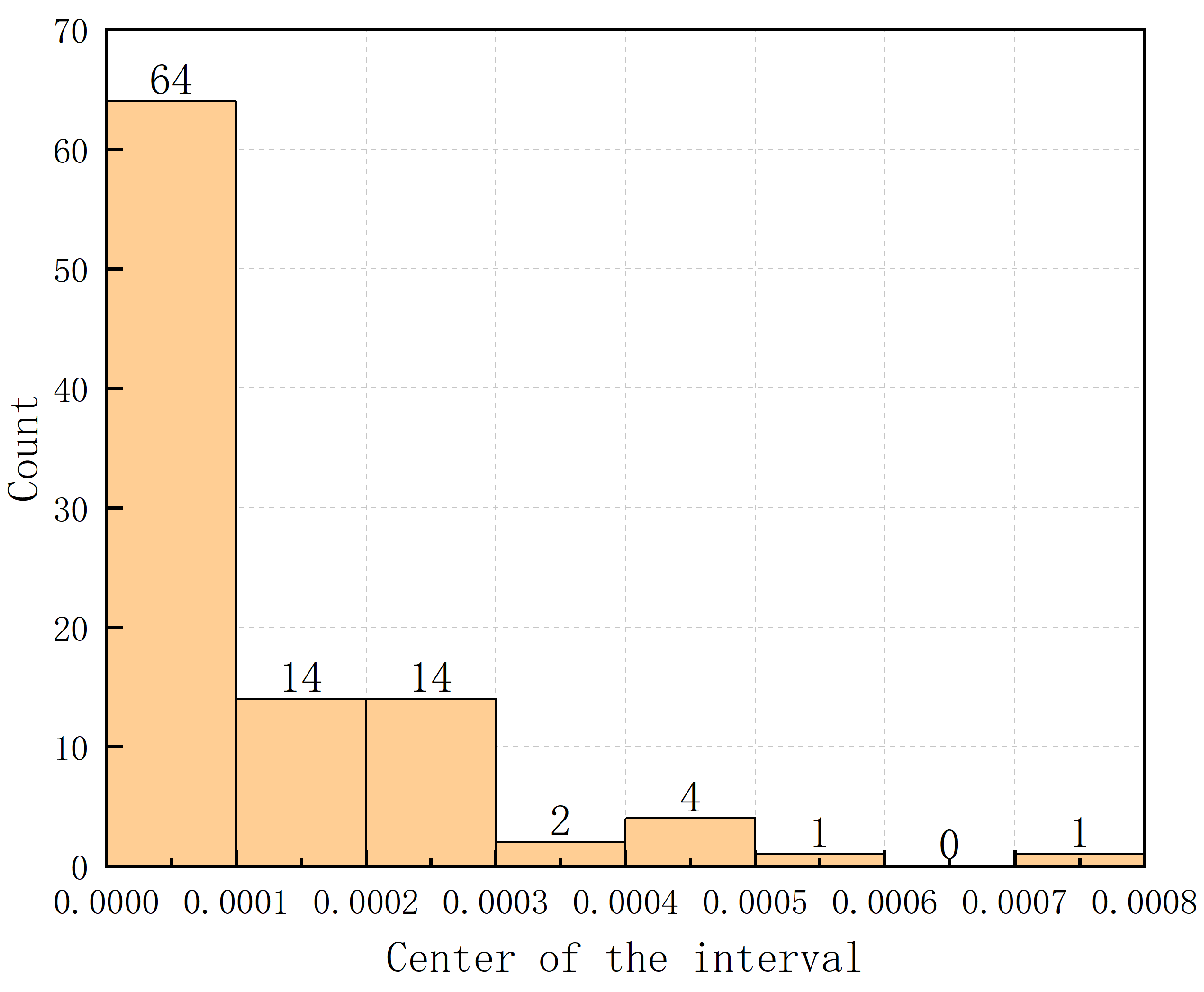
To further validate the conclusion that expert weights are inversely proportional to the corresponding distances, we randomly generated 100 datasets and analyzed their “deviation”. The number of alternatives and criteria in each decision group were randomly selected from the interval
. Similarly, the number of experts was randomly chosen within this range, subject to the condition that it does not exceed the product of the number of alternatives and criteria, ensuring that the matrix columns are full rank and the expert weights exist and are unique. These 100 datasets represent abstractions of distinct decision problems, each characterized by different numbers of decision makers, alternatives, and evaluation criteria (see
Table 5). We performed a statistical analysis of the expert weights computed for each case. The results provide evidence of both the validity and generalizability of our conclusions. Moreover, the heterogeneous levels of agreement among decision makers across these problems capture the range of consensus and conflict scenarios that can arise in practice. Such variability can significantly influence a model’s effectiveness and fairness in real-world decision making. By examining outcomes over all 100 cases, we further demonstrate the robustness and broad applicability of the proposed weight-determination method.
Under these conditions, we generated 100 datasets and conducted numerical experiments to compute the corresponding expert weights. We then calculated the distance to the “overall consistent scoring point” and the product of the two. The “deviation” for each dataset is summarized in
Table 6, and the frequency distributions for the optimal expert weights and mean weights are shown in
Figure 3 and
Figure 4. As illustrated in
Figure 3, the “deviation” of the decision is relatively small across multiple experiments, suggesting that, accounting for the inevitable errors in numerical experiments, expert weights are inversely proportional to the distances. This confirms that the weights obtained by the model exhibit “perfect rationality”.


