An Integrated Implementation Framework for Warehouse 4.0 Based on Inbound and Outbound Operations

Abstract

Warehouse 4.0 adopts automation, IoT, and big data technologies to establish an intelligent warehousing system for efficient, real-time management of storage, handling, and picking. Addressing challenges like unreasonable storage allocation and inefficient order fulfillment, this paper presents an integrated framework that utilizes swarm intelligence algorithms and collaborative scheduling strategies to optimize inbound/outbound operations. First, for inbound processes, an algorithm-driven storage allocation model is proposed to solve stacker crane scheduling problems. Then, for outbound operations, a “1+N+M” mathematical model is developed, optimized through a three-stage algorithm addressing order picking and distribution scheduling. Finally, a case study of an industrial warehouse validates the proposed methods. The improved mayfly algorithm demonstrates excellent performance, achieving 64.5–74.5% faster convergence and 20.1–24.7% lower fitness values compared to traditional algorithms. The three-stage approach reduces order fulfillment time by 12% and average processing time by 1.8% versus conventional methods. These results confirm the framework’s effectiveness in enhancing warehouse operational efficiency through intelligent automation and optimized resource scheduling.

1. Introduction

In the era of economic globalization and supply chain integration, the characteristics of modern warehousing logistics are constantly evolving and innovating [1]. Smart Warehouse Logistics (SWL) has become an important component of “Industry 4.0” [2,3]. Warehouse 4.0 refers to the construction of a highly automated and intelligent warehousing system by integrating advanced technologies such as automation, the Internet of Things (IoT), big data, and artificial intelligence. The significance of Warehouse 4.0 lies in the comprehensive digitalization and intelligentization of warehousing operations through the deep integration of next-generation intelligent manufacturing technologies [4]. This enhances operational efficiency and accuracy, reduces labor and operational costs, and improves the responsiveness and flexibility of the supply chain, thereby providing enterprises with more efficient, reliable, and competitive logistics solutions.

Modern warehouses face many challenges such as inadequate accuracy in inventory management, extended order fulfillment cycles, low utilization rate of three-dimensional space, and lagged response to demand fluctuations. Inventory inaccuracies can trigger the “bullwhip effect,” causing information distortion and cost amplification across all supply chain segments; delays in order processing directly diminish customer experience, subsequently impacting the enterprise’s market competitiveness. In response to these challenges, intelligent upgrading of warehouse systems has become imperative. As a core component of intelligent logistics systems, the construction of efficient storage allocation mechanisms and dynamic picking scheduling strategies is particularly crucial [5]. This requires the integration of advanced algorithm models into the Warehouse Management System (WMS), such as swarm intelligence optimization algorithm-driven storage allocation models and planning systems incorporating multi-objective optimized paths, to achieve optimal resource allocation and intelligent coordination of operational workflows [6,7]. Addressing the complex issues of storage system allocation and integrated scheduling for inbound and outbound operations not only improves the efficiency of individual warehousing nodes but also helps establish a resilient supply chain ecosystem.

Based on the above background, this paper focuses on intelligent warehousing based on the Industrial Internet of Things (IIoT) information perception and transmission architecture. It studies autonomous allocation technology for storage locations in multiple stacker parallel operations and joint scheduling for outbound order picking and distribution for diverse demands. The main contributions of this paper are as follows:

(1)

An integrated implementation framework is proposed to use swarm intelligence and joint scheduling strategies to address inbound and outbound operations. This optimizes warehouse processes, reduces error rates and operational costs, and enhances the overall supply chain’s responsiveness and competitiveness.

(2)

An allocation algorithm for goods locations is proposed, which can assign goods locations based on order goods information. This improves the operational efficiency of goods location allocation, effectively reduces the operation time of automated warehouses, and enhances the efficiency of goods inbound and outbound processes. The implementation of this algorithm requires collaboration with hardware and software to achieve autonomous storage location allocation.

(3)

A combined warehousing order picking and distribution operation is proposed, which performs batch order picking and rational distribution route planning. This improves the inefficiency of the First-In-First-Out (FIFO) model, enhances overall order fulfillment efficiency, optimizes warehouse resources, and ensures the efficient operation of the intelligent warehouse cloud service system.

The rest of this paper is organized as follows: Section 2 reviews the related literature, Section 3 describes the research problem and its implementation framework, Section 4 proposes the autonomous storage location allocation technology based on an improved mayfly algorithm (IMA), Section 5 presents the joint scheduling technology for outbound order picking and distribution based on a three-stage algorithm, Section 6 validates the proposed framework for storage location allocation and picking joint scheduling through a case study, and Section 7 concludes the paper and discusses the limitations of the proposed method.

2. Literature Review

An effective storage location allocation scheme is critical for enhancing warehousing efficiency, optimizing access processes, and achieving intelligent warehouse management [6,7]. Current research primarily focuses on modeling objectives, including storage space utilization, operational costs, and rack stability [8]. For example, Liu et al. established an MIPP-AS/RS replenishment model using queuing theory, calculating task probability density through the Chebyshev theorem to optimize multi-channel storage system responsiveness [9]. Shoaee et al. developed a mathematical model for transfer warehouse layout, integrating NSGA-II and MOGWO algorithms to minimize material movement distance while maximizing spatial utilization [10]. Wan et al. constructed a multi-objective model based on high-frequency prioritization and associated storage principles, employing an improved genetic-particle swarm optimization (IGPSO) algorithm to enhance manual picking zone efficiency by 19.3% [11]. Gao et al. created a synchronized storage allocation model that balanced high-bay warehouse capacity ratios, improving storage efficiency by 19.3% [12]. Ma et al. proposed a dual-objective model (SPEA-II algorithm) achieving 15% reduction in unit cargo damage and 28% decrease in stacker operating time [13]. Islam et al. proposed an associated storage allocation method (CBSLA), with simulations demonstrating a 29–41% reduction in order-picking travel distance [14]. Rungjaroenporn et al. developed a time-minimization model for multi-warehouse allocation, proving that the flower pollination algorithm outperformed genetic algorithms in both fitness value (18.7% improvement) and convergence speed (34% acceleration) [15]. Xu et al. transformed static allocation into multi-stage dynamic processes using genetic algorithms to adjust grid status in real time, boosting e-commerce warehouse throughput by 22% [16]. Zhang et al. designed an artificial population algorithm for efficiency–stability–classification tri-objective optimization, providing new pathways for logistics automation [17]. De Puiseau employed Deep Reinforcement Learning (DRL) to derive an appropriate storage location assignment strategy aimed at reducing transportation costs within the warehouse [18]. Leng et al. implemented a digital twin system enabling physical warehouse synchronization through real-time data-driven joint storage optimization decisions [19]. The differences between the mayfly algorithm (MA) and improved mayfly algorithm (IMA), particle swarm optimization (PSO), and genetic algorithm (GA) are shown in

Table 1. Comparison of various algorithms.

Algorithm	Description	Advantages	Disadvantages
GA	An optimization algorithm that simulates natural selection and genetic mechanisms	High robustness	Complexity in encoding and decoding processes
PSO	Swarm intelligence-based optimization algorithm that searches for optimal solutions through collaboration and competition among particles	Strong global search capability	Sensitivity to parameter settings
MA	An optimization algorithm inspired by the biological behaviors of mayflies	Simple and easy to understand	Slower convergence speed
IMA	Introduces adaptive dynamic inertia weight factor, Lévy flight strategy, and golden sine division factor	Faster convergence speed, high randomness, and stability of solutions	Relatively higher algorithm complexity, and potentially complex parameter tuning

.

Research on large-scale order picking and distribution efficiency optimization focuses on parallel stacker operations and multi-vehicle collaborative scheduling strategies. Gao et al. established a dual-scenario order sequencing model under the constraints of order quantity, vehicle capacity, and processing time, employing heuristic algorithms to determine optimal scheduling schemes for identical processing/delivery time conditions [20]. Li et al. developed a single-machine production to multi-customer delivery integrated scheduling model utilizing genetic algorithms to minimize transportation costs and customer waiting time simultaneously [21]. Rasti-Barzoki et al. introduced an innovative joint scheduling framework integrating delivery time, production batches, and fulfillment costs, achieving 23% reduction in delayed operations and 18% decrease in comprehensive costs [22]. Suppini et al. proposed dynamic picking strategies through warehouse shape analysis and I/O point optimization, reducing picker travel distances by 15–32% [23]. Schumann et al. constructed a picking performance calculation model using mobility data, with case studies demonstrating 27% efficiency improvement through optimized picking surface layouts [24]. Modenov et al. formulated a production–inventory–transportation linear programming model, verifying a 21% operational cost reduction through multi-process coordination [25]. Han et al. designed an integrated production–inventory–distribution scheduling system, developing a pseudo-polynomial time algorithm that reduced backlogged operations by 34% [26]. Czerniachowska et al. proposed two solutions: a two-step mathematical heuristic addressing sequence-constrained order sorting and a CPLEX-based task allocation model that shortened order completion time by 19% through optimized picker assignments [27,28]. Tsang et al. created a multi-temperature IoT-enabled scheduling model for B2C fresh produce delivery, applying two-phase multi-objective genetic algorithms to enhance order processing capacity by 41% while improving customer satisfaction by 29% [29]. Mukherjee et al. developed a mixed-integer linear programming model to determine optimal pallet machine configurations, with experiments showing 28% resource utilization improvement [30].

In summary, existing storage location allocation methods primarily focus on how to allocate static vacant locations to items to be stored, with relatively little research on the autonomous allocation of storage locations for partitioned parallel storage operations based on warehouse perception data. Moreover, some existing research models consider only a single objective function, while some multi-objective optimization algorithms suffer from slow convergence speeds. Therefore, it is of great significance to use high-performance optimization algorithms to achieve partitioned parallel storage operations in warehousing. Current research results on picking and distribution operations mainly focus on order batch picking and vehicle routing planning, with fewer results on the joint scheduling of order batch picking and distribution. Additionally, the picking and distribution stages often make independent decisions, making it difficult to achieve optimal efficiency for the overall warehouse logistics system [2,10,26,31]. Therefore, considering the joint scheduling of picking and distribution in warehouse logistics to address the above issues is important.

3. Problem Description and Its Implementation Framework

3.1. Problem Description

The first step in warehouse inbound operations is to clarify the task information for the inbound order. Suppose that the input buffer and output buffers of the k-th aisle are equipped with RFID readers $C_1^k$ and $C_2^k$. $C_1^k$ monitors the goods entering the aisle buffer, and the original event sensed by $C_1^k$ increases the quantity of goods; $C_2^k$ monitors the goods leaving the aisle buffer, and the original event sensed by $C_2^k$ decreases the quantity of goods. As goods equipped with RFID electronic tags are transported to the designated aisle buffer via the conveyor, RFID readers detect and read the electronic product code (EPC) of the tags. A tag’s attribute information includes the goods’ name, owner’s name, carton specifications, and inbound time, among other details, collectively represented as follows in

Table 2. Introduction to system parameters.

Name	Function
$G\_name$	the goods’ name
$O\_name$	the supplier’s name
B	the carton specifications
$E\_time$	the inbound time
R	the outbound frequency
W	the weight of the goods
K	the type of goods
N	the quantity of goods
$C\_I$	the customer information
$G\_I$	the goods information
$D\_I$	the distribution vehicle information
$C\mathrm{ustom}\_name$	the customer’s name
$C\mathrm{ustom}\_tel$	the customer’s contact information
$C\mathrm{ustom}\_location$	the customer’s location
$C\mathrm{ustom}\_goods\_num$	the quantity of goods ordered by the customer
$Goods\_name$	the name of the goods
$Goods\_code$	the code of the goods
$Goods\_coordinate$	the coordinates of the goods on the shelf
$Delivery\_code$	the code of the distribution vehicle
$Delivery\_state$	the state of the distribution vehicle
$Delivery\_capacity$	the maximum capacity of the distribution vehicle

:

$$Tag=\left\{G\_name,O\_name,B,E\_time,R,W,K,N\right\},$$

(1)

where $G\_name$ denotes the goods’ name, $O\_name$ is the supplier’s name, B denotes the carton specifications, $E\_time$ is the inbound time, R denotes the outbound frequency, W is the weight of the goods, K denotes the type of goods, and N is the quantity of goods.

The inbound and outbound operation process is shown in Figure 1.

The outbound order $Order\_E\mathrm{x}$ is described as follows:

$$Order\_Ex=\left\{C-I,G-I,D-I\right\},$$

(2)

where $C\_I$ denotes the customer information, $G\_I$ denotes the goods information, and $D\_I$ denotes the distribution vehicle information.

Further detailing the outbound order description:

$$C-I=\left\{Custom\_name,Custom\_tel,Custom\_location,Custom\_goods\_num\right\},$$

(3)

where $C\mathrm{ustom}\_name$ denotes the customer’s name, $C\mathrm{ustom}\_tel$ denotes the customer’s contact information, $C\mathrm{ustom}\_location$ denotes the customer’s location, and $C\mathrm{ustom}\_goods\_num$ denotes the quantity of goods ordered by the customer.

$$G-I=\left\{Goods\_name,Goods\_code,Goods\_coordinate\right\},$$

(4)

where $Goods\_name$ denotes the name of the goods, $Goods\_code$ denotes the code of the goods, and $Goods\_coordinate$ denotes the coordinates of the goods on the shelf.

$$D-I=\left\{Delivery\_code,Delivery\_state,Delivery\_capacity\right\},$$

(5)

where $Delivery\_code$ denotes the code of the distribution vehicle, $Delivery\_state$ denotes the state of the distribution vehicle, and $Delivery\_capacity$ denotes the maximum capacity that the distribution vehicle.

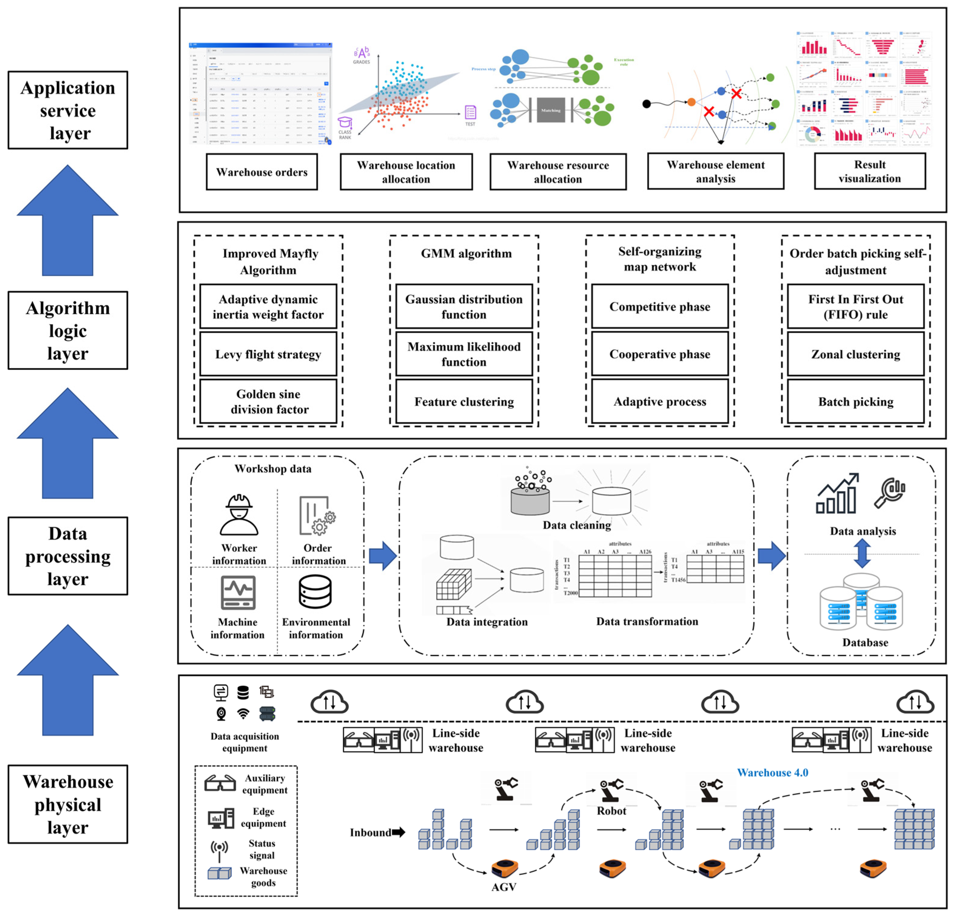
3.2. Integrated Implementation Framework for Warehouse 4.0-Based Inbound and Outbound Operations

The integrated implementation framework for Warehouse 4.0-based inbound and outbound operations is shown in Figure 2. The framework is divided into four layers. The warehouse physical layer demonstrates the specific process of warehouse inbound and outbound operations. The data processing layer cleans and integrates the collected warehouse data, providing the foundation for data analysis. The algorithm logic layer showcases the core of the improved mayfly algorithm and the three-stage algorithm. The application service layer displays the specific applications of this framework.

3.3. Process of Inbound and Outbound Operations

After the inbound operation is issued, information about the goods to be shelved and the current vacant storage locations are called from the database as input variables and imported into the intelligent warehouse inbound storage location allocation mathematical model. The improved mayfly algorithm is used for optimizing and solving the results of inbound storage location allocation. Finally, the storage locations of the goods in the outbound orders and the customer information in the orders are analyzed. The Gaussian clustering algorithm is used for clustering analysis, and the self-organizing neural network algorithm is employed for path planning. The results are then used to adjust and optimize the picking sequence, achieving optimal overall efficiency for warehouse outbound operations.

Storage location allocation and picking scheduling in warehouse operations are closely related. Location allocation determines the storage position of goods in the warehouse, directly affecting the length and efficiency of the picking path. Picking scheduling, on the other hand, optimizes the picking sequence and path according to order requirements and location distribution to reduce operation time and costs. Through joint scheduling, storage location allocation and picking strategies can be collaboratively optimized, thereby improving the overall efficiency of warehouse operations, reducing operational costs, and enhancing order processing speed.

4. Inbound Storage Location Allocation Based on Improved Mayfly Algorithm

4.1. Mathematical Model for Storage Location Allocation

4.1.1. Objective Function

The following assumptions are established:

(1)

Goods are stored in containers, which are placed at the center of the pallets in storage bays;

(2)

Each storage bay within the high-rise racking system is of the same size, and only one container can be stored in each bay;

(3)

The initial position of the aisle stacker crane is at the I/O port. It moves at a constant speed both horizontally and vertically, and the time required for receiving signals, turning, and picking up goods is neglected;

(4)

Goods are accessed while placed on pallets;

(5)

The waiting time for goods to be stored in the warehouse is ignored;

(6)

Each storage location stores only one type of commodity, taking into account the volume of the commodity and the storage space of the location, i.e., zoning based on volume;

(7)

In the storage location allocation scenario during storage operations, on a rack where several storage bays are already occupied, a reasonable storage location is allocated for the goods from the vacant bays.

The parameters and variables involved in the mathematical model are defined as follows:

p: Number of rows of racks

q: Number of columns of racks

τ: Number of tiers of racks

i: The i-th goods, where $i=\left\{1,2,\cdots \right\}$

$m_i$: Mass of goods i

$R_i$: Outbound frequency of goods i

$O_i$: Owner’s priority level of goods i

$P_i$: Storage cycle of goods i

B: Container specification, where $B=\left\{1,2,3,4,5\right\}$

n: The n-th stacker crane, where $n=\left\{1,2,\cdots ,M\right\}$

$G_{xyz}$: Storage location in the x-th row, y-th column, and z-th tier

$C_{xyz}$= ($X_{xyz},Y_{xyz},Z_{xyz}$): Three-dimensional coordinates of storage location $G_{xyz}$

A: Current set of storage locations under dynamic warehouse updates

$A_{ixyz}$: Indicates whether goods i are placed in the x-th row, y-th column, and z-th tier

$S\left(C_{xyz}\right)$: Distance traveled horizontally by the conveyor

$T_b\left(C_{xyz}\right)$: Time consumed for horizontal transportation of the storage location by the conveyor

$T_n\left(C_{xyz}\right)$: Time consumed for the operation of the n-th stacker crane

$T_d\left(C_{xyz}\right)$: Time consumed for parallel operations of stacker cranes

$v_{h1}$: Speed of the horizontal conveyor

$v_{h2}$: Horizontal movement speed of the stacker crane

$v_v$: Vertical movement speed of the stacker crane

L: Length and width values of the storage bay

H: Height value of the storage bay

Considering the efficiency of goods entering and leaving the warehouse and the stability of the shelves, two objective functions are established, as shown in Equations (9) and (10).

1.

Depending on whether the rack is in an odd or even row, the formula for the conveyor transport distance varies, and the floor function is used to represent the conveyor transport distance [13]. The operational time of the conveyor can be expressed as follows:

$$T_b(C_{xyz})={\displaystyle \frac{S(C_{xyz})}{v_{h1}}}={\displaystyle \frac{x+[\frac{x}{2}]\times L}{v_{h1}}},$$

(6)

where $T_b(C_{xyz})$ is the time consumed by the conveyor for horizontal transportation of the slot, $S(C_{xyz})$ is the distance traveled by the conveyor in the horizontal direction, ${\mathrm{v}}_{h1}$ is the speed of the conveyor, and L is the length and width value of the slot.

Since the stacker can move simultaneously in both the vertical and horizontal directions, the max function is used to find the larger value of the operation times in the two directions. Thus, the operation time of the nth stacker is

$$T_n(C_{xyz})=\max \left\{{\displaystyle \frac{y\times L}{v_{h2}}},{\displaystyle \frac{\left(z-1\right)\times H}{v_{\mathrm{v}}}}\right\},$$

(7)

where $T_n(C_{xyz})$ is the time consumed by the nth stacker during operation, ${\mathrm{v}}_{h2}$ is the horizontal movement speed of the stacker, H is the height value of the slot, and ${\mathrm{v}}_v$ is the vertical movement speed of the stacker.

Considering that the stackers in each aisle are operating in parallel, the time $T_d\left(C_{xyz}\right)$ consumed for an inbound order task by M stackers is

$$T_d(C_{xyz})=\max \left\{T_n(C_{xyz})\right\},n=1,2\mathbf{·}\mathbf{·}\mathbf{·}\mathbf{·}\mathbf{·}\mathbf{·}M.$$

(8)

Thus, the first objective function is established as follows:

$$\min f_1={\displaystyle \sum _i{\displaystyle \sum _x^p{\displaystyle \sum _y^q{\displaystyle \sum _z^{\tau }\left[T_d(C_{xyz})+T_b(C_{xyz})\right]}}}}\times {\displaystyle \frac{R_i\times O_i}{P_i}}\times A_{ixyz},$$

(9)

where $R_i$, $O_i$, and $P_i$ denote the estimated outbound frequency, owner level, and storage cycle of goods i, respectively; and $A_{ixyz}$ denotes whether goods i are positioned at position (x, y, z).

2.

The second objective function aims to minimize the sum of the products of the weights of all goods and the levels of their respective assigned positions.

$$\min f_2={\displaystyle \sum _i{\displaystyle \sum _x^p{\displaystyle \sum _y^q{\displaystyle \sum _z^{\tau }{m}_i}}}}\times z\times A_{ixyz},$$

(10)

where $m_i$ denotes the weight of goods i.

4.1.2. Constraints

$${\displaystyle \sum _i{A}_{ixyz}}\le 1,\forall i,x,y,z,$$

(11)

$${\displaystyle \sum _{x=1}^p{\displaystyle \sum _{y=1}^q{\displaystyle \sum _{z=1}^{\tau }{A}_{ixyz}}}}=1,\forall i,$$

(12)

$$\left\{\begin{array}{l}1\le x\le p, x\in N\\ 1\le y\le q, y\in N\\ 1\le z\le \tau , z\in N\end{array}\right.,$$

(13)

$$1\le n\le M,n\in N.$$

(14)

Equation (11) indicates that each storage location can only store one item; Equation (12) states that each item must be stored in a specific storage location; Equation (13) expresses that the coordinates of the storage location cannot exceed the maximum dimensions of the racking system; and Equation (14) denotes that the number of stacker cranes cannot exceed the maximum number of resources available in the warehouse.

The weight allocation method is used to assign two influencing factors ${\theta }_1$ and ${\theta }_2$ to the objective functions $f_1$ and $f_2$. The weight proportions of ${\theta }_1$ and ${\theta }_2$ can be adjusted according to practical operations, enabling dynamic planning of the storage process, i.e.,

$$\min f={\theta }_1{f}_1+{\theta }_2{f}_2,$$

(15)

$$\left\{\begin{array}{l}{\theta }_1+{\theta }_2=1\\ 0\le {\theta }_1\le 1\\ 0\le {\theta }_2\le 1\end{array}\right..$$

(16)

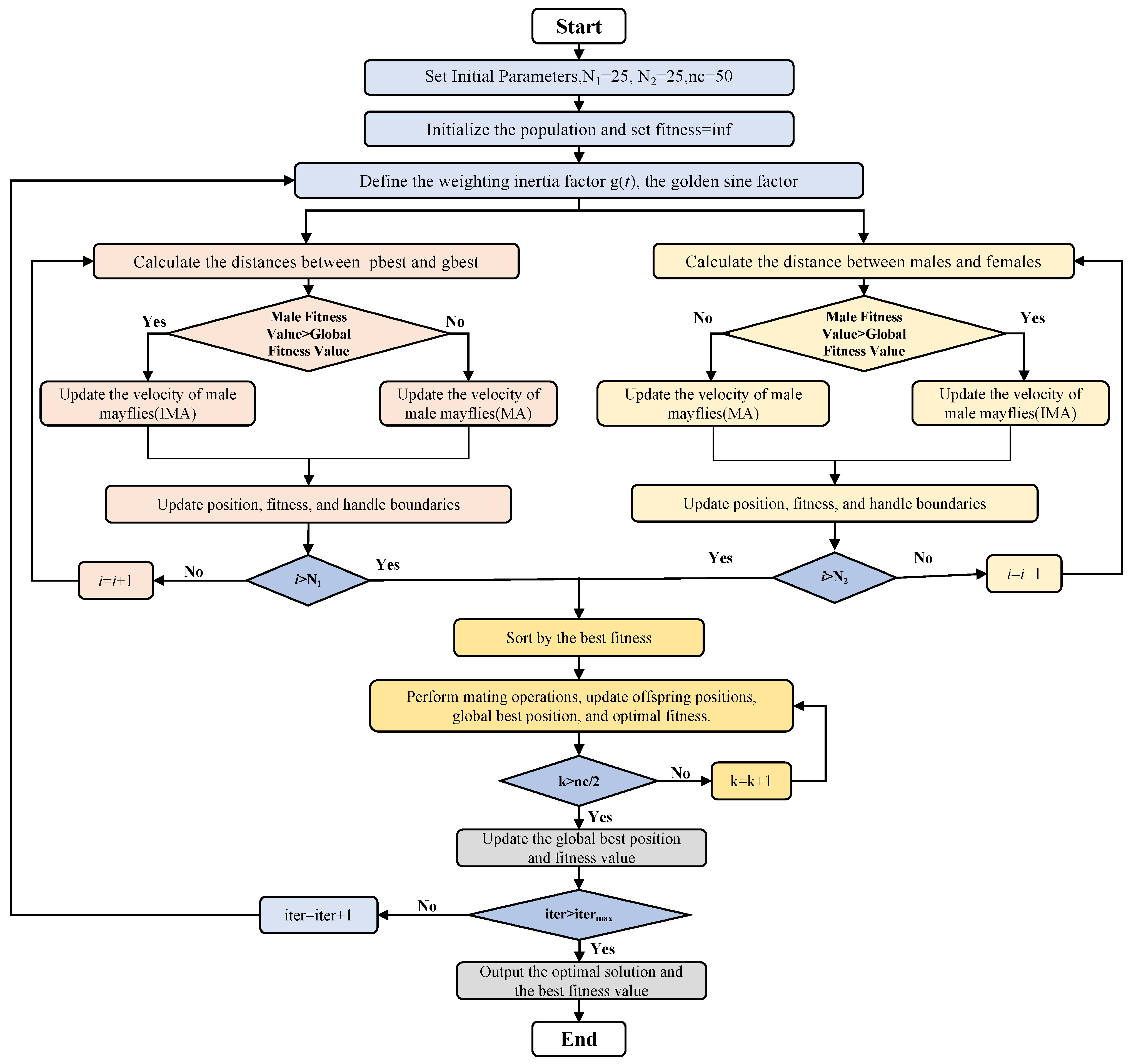
4.2. Autonomous Location Allocation Based on Improved Mayfly Algorithm

The paper introduces an improved mayfly algorithm, which primarily aims to adaptively adjust the variable parameter factors in the mayfly algorithm to enhance both the randomness and stability of the solutions. The following three improvements have been implemented in MA:

(1)

Introduction of the Adaptive Dynamic Inertia Weight Factor

The formula for the nonlinear inertia weight factor is as follows:

$$g\left(t\right)={\displaystyle \frac{e^{\frac{2\left(1-iter\right)}{ite{r}_{max}}}-e^{\frac{-2\left(1-iter\right)}{ite{r}_{max}}}}{e^{\frac{2\left(1-iter\right)}{ite{r}_{max}}}+e^{\frac{-2\left(1-iter\right)}{ite{r}_{max}}}}},$$

(17)

where g denotes the inertia weight, iter is the iteration coefficient, and ${iter}_{max}$ is the maximum iteration coefficient.

(2)

Introduction of the Lévy Flight Strategy

The expression for the Lévy distribution is as follows:

$$Levy\left(s,\lambda \right)\approx s^{-\lambda },$$

(18)

where s denotes the random step length; λ ∈ (1,3].

After introducing the Lévy flight strategy, the velocity update expression for male mayflies in the mayfly algorithm is

$$v_{ij}^{t+1}=\left\{\begin{array}{l}g\times v_{ij}^t+a_1{e}^{-\beta r_p^2}\left(Levy\oplus pbes{t}_{ij}-x_{ij}^t\right)+a_2{e}^{-\beta r_g^2}\left(gbes{t}_{ij}-x_{ij}^t\right),\\ \hspace{1em}\hspace{1em}\hspace{1em}\hspace{1em}\hspace{1em}\mathrm{if} f\left(x_i\right)>f\left(gbest\right)\\ g\times v_{ij}^t+d\times r, \mathrm{if} f\left(x_i\right)\le f\left(gbest\right)\end{array}\right.,$$

(19)

where $v_{ij}^t$ is the velocity of individual i in the j dimension at time t; $a_1$ and $a_2$ are the population learning coefficient and individual learning coefficient, respectively; $\beta$ is the visibility coefficient of the mayfly; Levy represents the Lévy flight factor; ${pbest}_{ij}$ is the historical optimal position of mayfly i; gbest is the global best position; $x_{ij}^t$ is the position of individual i in the j dimension at time t; $r_p$ and $r_g$ denote the distances to ${pbest}_{ij}$ and gbest, respectively; and d is the dance coefficient.

(3)

Introduction of the Golden Sine Division Factor

The initialization boundary can be expressed as follows:

$$V_i=c\times \left(ub-lb\right)+lb,$$

(20)

where $V_i$ denotes the position of individual i; ub and lb denote the upper and lower boundaries, respectively; and $c\in [0,1]$.

The adaptive adjustment formula for the Golden Sine Division Coefficient is as follows:

$$\left\{\begin{array}{l}{c}_1=a\times \left(1-h\right)+bh\\ c_2=ah+b\left(1-h\right)\end{array}\right.,$$

(21)

where $c_1$ and $c_2$ are the Golden Sine Division Coefficients; a and b are the initial values of the Golden Ratio Coefficients; and h is the Golden Ratio.

In order to ensure that the population completes traversal in all spaces during the cycle, set $a=\pi$, $b=-\pi$. The Golden Ratio is applied to the position update of the mayfly, and its formula is

$$V_i^{t+1}=V_i^t\times \left|\sin \left(r_1\right)\right|-r_2\times \sin \left(r_1\right)\times \left|c_1{D}_i^t-c_2{V}_i^t\right|,$$

(22)

where $D_i^t$ is the optimal position of mayfly i at iteration t; $r_1\in \left[\mathrm{0,2}\mathsf{\pi }\right]$, $r_2\in [0,\mathsf{\pi }]$.

The Golden Ratio coefficient is applied to the mating process in the mayfly algorithm to generate offspring. That is, the optimal male and female mayflies perform a Golden Crossover to obtain offspring ${offs}_1$, while the second-best male and female mayflies obtain offspring ${offs}_2$. The formula for combining the offspring individuals in Gold-SA is

$$\left\{\begin{array}{l}off{s}_1=x_i^1\left|\sin \left(r_1\right)\right|-r_2\ast \sin \left(r_1\right)\ast \left|c_1\ast pbes{t}_x-c_2\ast x_i^t\right|\\ off{s}_2=y_i^1\left|\sin \left(r_1\right)\right|-r_2\ast \sin \left(r_1\right)\ast \left|c_2\ast pbes{t}_y-c_2\ast x_i^t\right|\end{array}\right.,$$

(23)

where $x_i^1$ and $y_i^1$ denote the initial positions of the male and female individuals in the i dimension and ${pbest}_x$ and ${pbest}_y$ denote the optimal positions of the male and female mayflies in the current iteration, respectively.

Based on the above three aspects, improvements are made to the MA algorithm. The flowchart of the IMA algorithm is shown in Figure 3.

5. Joint Scheduling of Outbound Order Picking and Distribution Based on a Three-Stage Algorithm

For outbound operations, a “1+N+M” model is developed. It refers to 1 distribution center, N customer orders, and M distribution vehicles. The outbound operation process of this mode is shown in Figure 4. Firstly, the order is split and merged based on the storage compartment where the goods are located, forming several picking batches. Because each aisle is operated by only one stacker crane, WMS assigns the picking task of each batch of goods to the stacker crane in the respective aisle. Then, after receiving instructions, the stacker crane autonomously updates the task list and moves the goods to the picking platform according to the task sequence instructions. Next, after completing the picking task, the stacker crane packages the order and assigns it to the designated delivery cart to perform the distribution task. The start time of the distribution task is the picking completion time of the last order in the distribution batch, the distribution time is the sum of the vehicle travel time and the customer service time, and the distribution end time is the time when the distribution vehicle returns to the distribution center after serving the customers on the route.

5.1. Mathematical Model for Joint Scheduling of Outbound Order Picking and Distribution

5.1.1. Objective Function

The following assumptions are established:

(1)

All distribution vehicles are identical, possessing a fixed capacity, and there is no limit on the number of vehicles.

(2)

Upon the vehicle’s arrival at the customer’s location, a fixed service time is required for each customer.

(3)

Once the distribution vehicle is fully loaded, it immediately begins distribution without any delay.

(4)

The initial position of the picking stacker is at the I/O port, and its horizontal and vertical movements are uniform, disregarding the time required for receiving signals, turning, and picking up goods.

(5)

Goods are stored and retrieved on pallets.

(6)

The time required for product verification and packaging during outbound operations is disregarded.

The parameters and variables involved in the mathematical model are defined as follows:

$M$: Set of orders, $M=\left\{1,2,\cdots ,m\right\}$

$M_0$: Set of orders, including the distribution center, $M_0=\left\{0,1,\cdots ,m\right\}$

$W$: Set of goods, $W=\left\{1,2,\cdots ,w\right\}$

$U$: Set of batches, $U=\left\{1,2,\cdots ,u\right\}$

$V$: Set of distribution vehicles, $V=\left\{1,2,\cdots ,v\right\}$

$q_p$: Quantity of goods in batch p, $p\in U$

$A_s$: Coordinate of the shelf where the goods are located, $A_s=(x_s,y_s,z_s)$, $s\in W$

$v_{h2}$: Horizontal movement speed of the stacker

$v_v$: Vertical movement speed of the stacker

$L$: Length and width of the storage slot

$H$: Height of the storage slot

$t_p^{start}$: Start time of picking for batch p, $p\in U$

$t_p^{pick}$: Time consumed for picking batch p, $p\in U$

$t_i^{complete}$: Completion time of picking for order i, $i\in M$

$t_l^{leave}$: Departure time of distribution vehicle l, $l\in V$

$t_l^{end}$: End time of distribution for vehicle l, $l\in V$

$Q_l$: Maximum capacity of distribution vehicle l, l ∈ V

$t_{i,j}$: Time consumed for a distribution vehicle to travel from point i to point j, $i,j\in M_0$

$T$: Service time required for each customer

$v_l$: Speed of the distribution vehicle

Based on the above assumptions and parameter definitions, a joint scheduling model for batch picking and outbound order distribution is established, with the objective of minimizing the total fulfillment time for picking and delivering all orders.

The set of orders $M=\left\{1,2,\cdots ,m\right\}$ contains several goods, with the set of goods represented as $W=\left\{1,2,\cdots ,w\right\}$. The storage coordinates of the goods are represented by the set $A_s$, where the coordinates of the shelf where goods are located are $A_s=(x_s,y_s,z_s)$, with $s\in W$. Based on the positions of the goods on the shelves, they are divided into several batches, and the set of batches is represented as $U=\left\{1,2,\cdots ,u\right\}$. Since the stacker moves simultaneously in both horizontal and vertical directions during operation, when an order is divided into several batches, the picking time $t_p^{pick}$ for batch p ∈ U can be expressed as the maximum execution time in the horizontal and vertical directions:

$$t_p^{pick}=\max \left\{{\displaystyle \frac{y_s\times L}{v_{h2}}},{\displaystyle \frac{\left(z_s-1\right)\times H}{v_{\mathrm{v}}}}\right\}.$$

(24)

As multiple batches of stackers operate concurrently, the total picking time for order i is defined as the maximum time among the picking batches:

$$t_i^{complete}=\max \left\{x_{ip}\left(t_p^{pick}+t_p^{start}\right)\right\}.$$

(25)

The start time $t_p^{start}$ of picking batch p is the time taken by the stacker to complete the previous p − 1 batches. Its expression is

$$t_p^{start}={\displaystyle \sum _{p-1}{t}_{p-1}^{pick}}.$$

(26)

The departure time $t_l^{leave}$ of the distribution vehicle is defined as the moment when the picking of all goods in the distribution order is completed:

$$t_l^{leave}=y_{pl}{t}_i^{complete}.$$

(27)

The time required for vehicle distribution comprises two components: the service time T and the travel time $t_{ij}$ from customer i to j. The coordinates ($C_x^i$, $C_y^i$) and ($C_x^j$, $C_y^j$) represent the two-dimensional map coordinates of customers i and j, respectively. The expression for $t_{ij}$ is

$$t_{ij}={\displaystyle \frac{\sqrt{{\left(C_x^i-C_x^j\right)}^2+{\left(C_y^i-C_y^j\right)}^2}}{v_l}}.$$

(28)

The expression for the distribution end time $t_l^{end}$ of vehicle l is

$$t_l^{end}=t_l^{leave}+{\displaystyle \sum _{i\in M}{\displaystyle \sum _{j\in M}{z}_{ijl}\left(T+t_{ij}\right)}}.$$

(29)

The objective function aims to minimize the fulfillment time for picking and delivering all outbound orders.

$$\min f=\max t_l^{end},l\in V.$$

(30)

5.1.2. Constraints

$$x_{ip}=\left\{\begin{array}{l}1,Order i is assigned to batch p\\ 0,\mathrm{else}\end{array}\right.\hspace{1em}\hspace{1em}i\in M,p\in U,$$

(31)

$$y_{ip}=\left\{\begin{array}{l}1,Batch p is assigned to vehicle l\\ 0,\mathrm{else}\end{array}\right.\hspace{1em}\hspace{1em}p\in U,l\in V,$$

(32)

$$z_{ijl}=\left\{\begin{array}{l}1,Coordinate points i and j are assigned to vehicle l\\ 0,\mathrm{else}\end{array}\right.\hspace{1em}\hspace{1em}i,j\in M,l\in V,$$

(33)

$${\displaystyle \sum _{p\in U}{y}_{pl}{q}_p\le Q_l},$$

(34)

$${\displaystyle \sum _{j\in M_0}{z}_{0jl}=1},\forall l\in V,$$

(35)

$${\displaystyle \sum _{j\in M_0}{z}_{i0l}=1},\forall l\in V,$$

(36)

$${\displaystyle \sum _{j\in M}{z}_{1jl}-{\displaystyle \sum _{j\in M}{z}_{i1l}=0}},\forall l\in V.$$

(37)

Equation (31) indicates that batch p is picked by only one stacker crane; Equation (32) indicates that batch p is delivered by only one vehicle; Equation (33) indicates that the distribution from customer coordinate i to j is carried out by only one vehicle; Equation (34) ensures that the sum of commodities in the batches assigned to vehicle l is less than the maximum capacity of the vehicle; and Equations (35)–(37) ensure that the vehicle, after completing its deliveries, returns to the warehouse center from which it departed.

5.2. Joint Scheduling Optimization Based on Three-Stage Algorithm

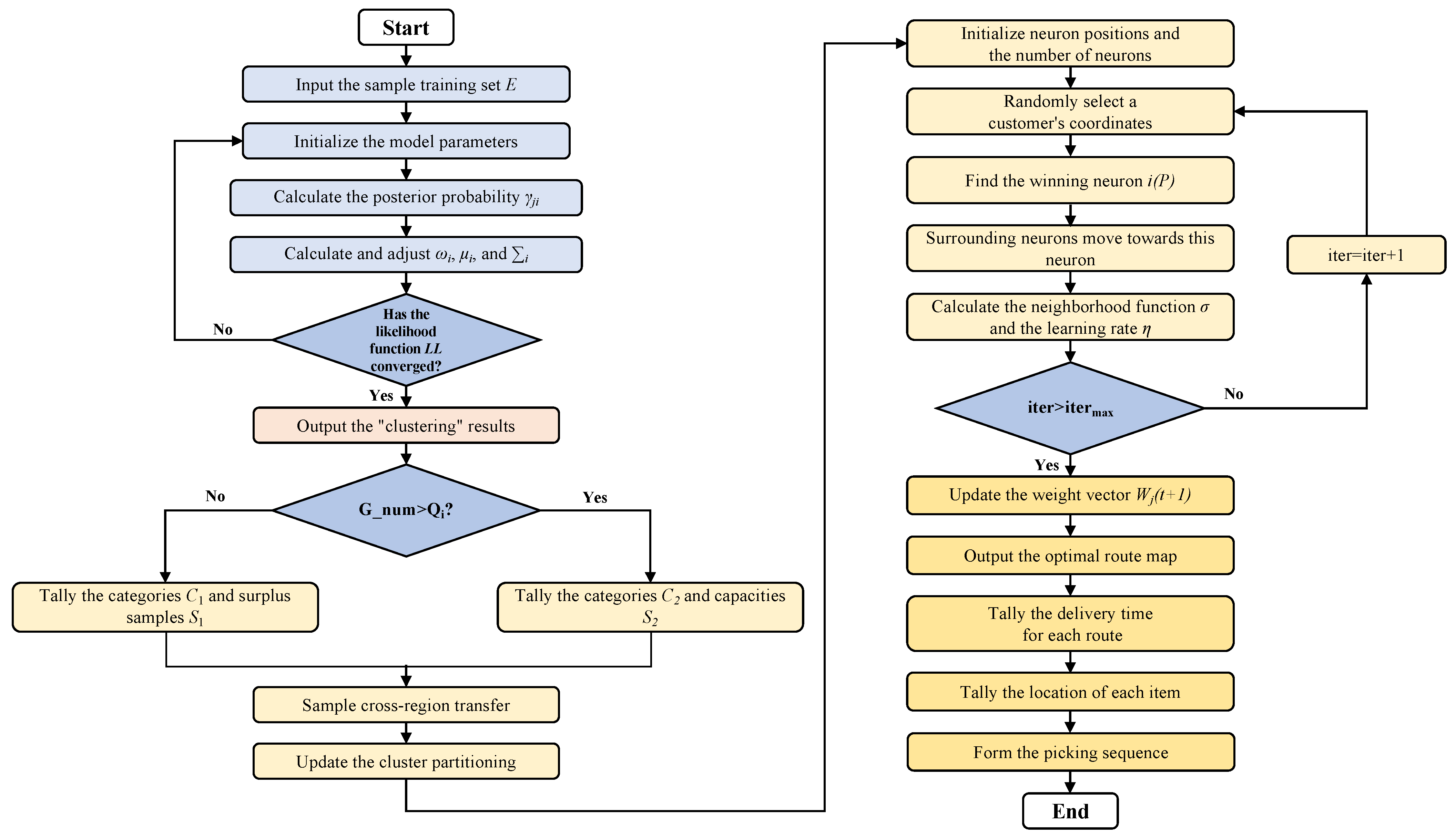
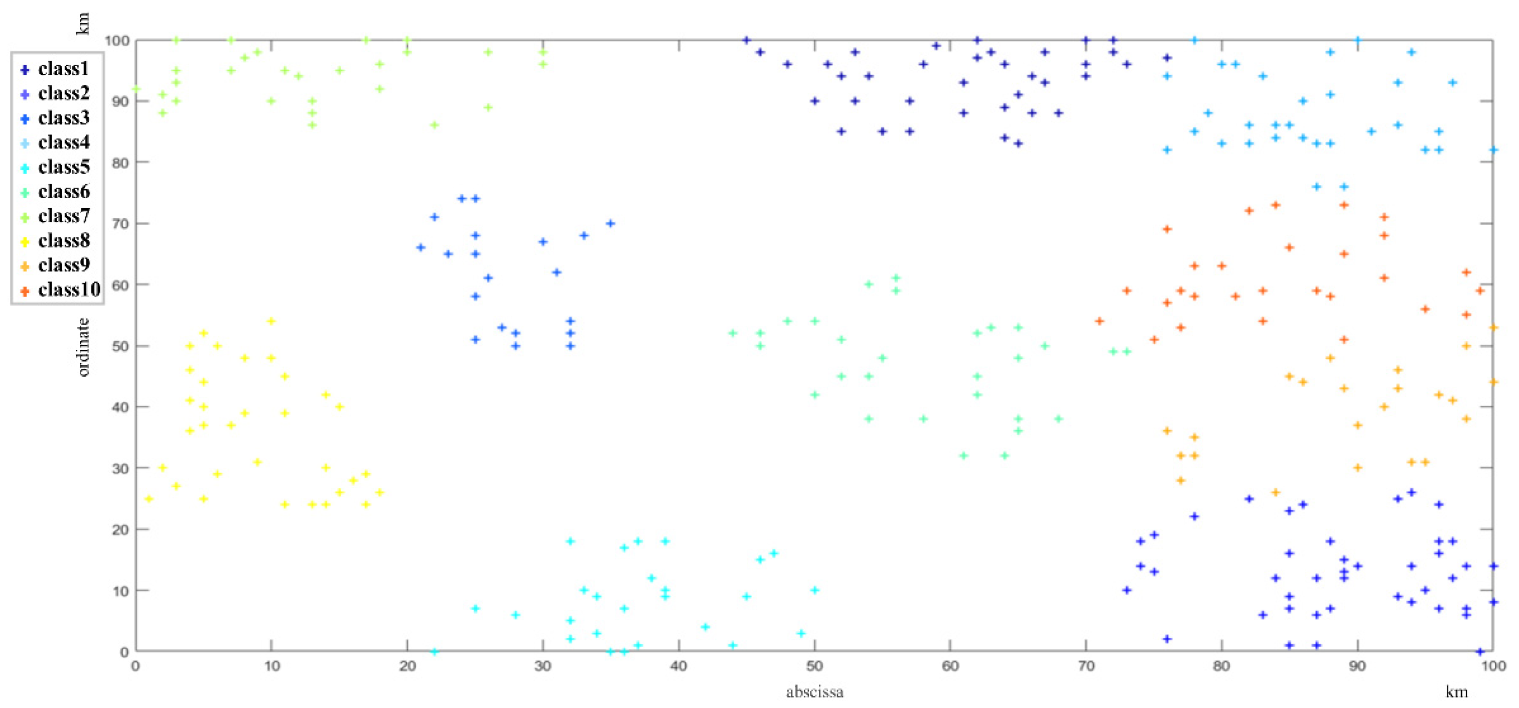
5.2.1. Constrained Outbound Order GMM Clustering

For a random vector x in the D-dimensional sample space χ, if x follows a Gaussian distribution, its probability density function p(x) is given by

$$p\left(x\right)={\displaystyle \frac{1}{{\left(2\pi \right)}^{\frac{D}{2}}\left|{\Sigma }^{1/2}\right|}}{e}^{-{\displaystyle \frac{1}{2}}\left(x-\mu \right){\Sigma }^{-1}{\left(x-\mu \right)}^T},$$

(38)

where μ is the D-dimensional mean vector, and Ʃ is the n × n covariance matrix.

To accurately represent each Gaussian distribution function, a mixing parameter ${\omega }_i$ is introduced, enabling the transformation of the Gaussian mixture model (GMM) into

$$p_G\left(x\right)={\displaystyle \sum _{i=1}^k{\omega }_{i}p\left(x|{\mu }_i,{\Sigma }_i\right)},$$

(39)

where $P_G\left(x\right)$ is the probability density function of the GMM, consisting of k mixture components; ${\omega }_i$ is the mixing coefficient, with ${\omega }_i$ > 0 and satisfying ${\sum }_{i=1}^k{\omega }_i=1$; ${\mu }_i$ and ${\Sigma }_i$ are the mean vector and covariance matrix of the i-th mixture component; and $p\left(x|{\mu }_i,{\Sigma }_i\right)$ is the probability density of the i-th mixture component.

The EM iterative algorithm is used to solve the GMM algorithm, and the process consists of the E-step and the M-step. In the E-step, it is assumed that the training set is $\mathrm{E}=\left\{x_1,x_2,\cdots x_m\right\}$, and the random variable $z_j\in \left\{1,2,\cdots k\right\}$ represents the Gaussian mixture component that generated the sample $x_j$. The prior probability $\mathrm{P}=\left\{z_j=i\right\}$ of $z_j$ corresponds to the mixing coefficient ${\omega }_i$. By the definition of Bayes, the posterior probability of $z_j$ is

$${\gamma }_{ji}=p\left(z_j=i|x_j,{\mu }_j,{\Sigma }_j\right)={\displaystyle \frac{p_G\left(z_j=i,x_j|\mu ,\Sigma \right)}{{\displaystyle \sum _{j=1}^i{p}_G\left(z_j=i,x_j|\mu ,\Sigma \right)}}}={\displaystyle \frac{{\omega }_{i}p\left(x_j|{\mu }_i,{\Sigma }_i\right)}{{\displaystyle \sum _{j=1}^i{\omega }_{i}p\left(x_j|{\mu }_i,{\Sigma }_i\right)}}}.$$

(40)

The M-step involves computing and adjusting the parameters ${\omega }_i$, ${\mu }_i$, and ${\Sigma }_i$. These parameters are updated based on the maximum likelihood principle, as shown in Equations (41)–(43).

$${\omega }_i={\displaystyle \sum _{j=1}^k\frac{{\gamma }_{ji}}{k}},$$

(41)

$${\mu }_i={\displaystyle \frac{{\displaystyle \sum _{j=1}^k{\gamma }_{ji}{x}_j}}{{\displaystyle \sum _{j=1}^k{\gamma }_{ji}}}},$$

(42)

$${\Sigma }_i={\displaystyle \frac{{\displaystyle \sum _{j=1}^k{\gamma }_{ji}\left(x_j-{\mu }_i\right){\left(x_j-{\mu }_i\right)}^T}}{{\displaystyle \sum _{j=1}^k{\gamma }_{ji}}}}.$$

(43)

When the error in the maximum likelihood function LL(E) from Equation (44) reaches its minimum after two iterations, the E-step and M-step terminate. The final cluster assignments are then made according to Equation (45) and the Gaussian mixture model.

$$LL\left(E\right)=\ln \left({\displaystyle \prod _{j=1}^m{p}_G\left(x_j\right)}\right)={\displaystyle \sum _{j=1}^m\ln \left({\displaystyle \sum _{i=1}^k{\omega }_{i}p\left(x_j|{\mu }_i,{\Sigma }_i\right)}\right)},$$

(44)

$${\omega }_j=\arg \max \left({\gamma }_{ji}\right).$$

(45)

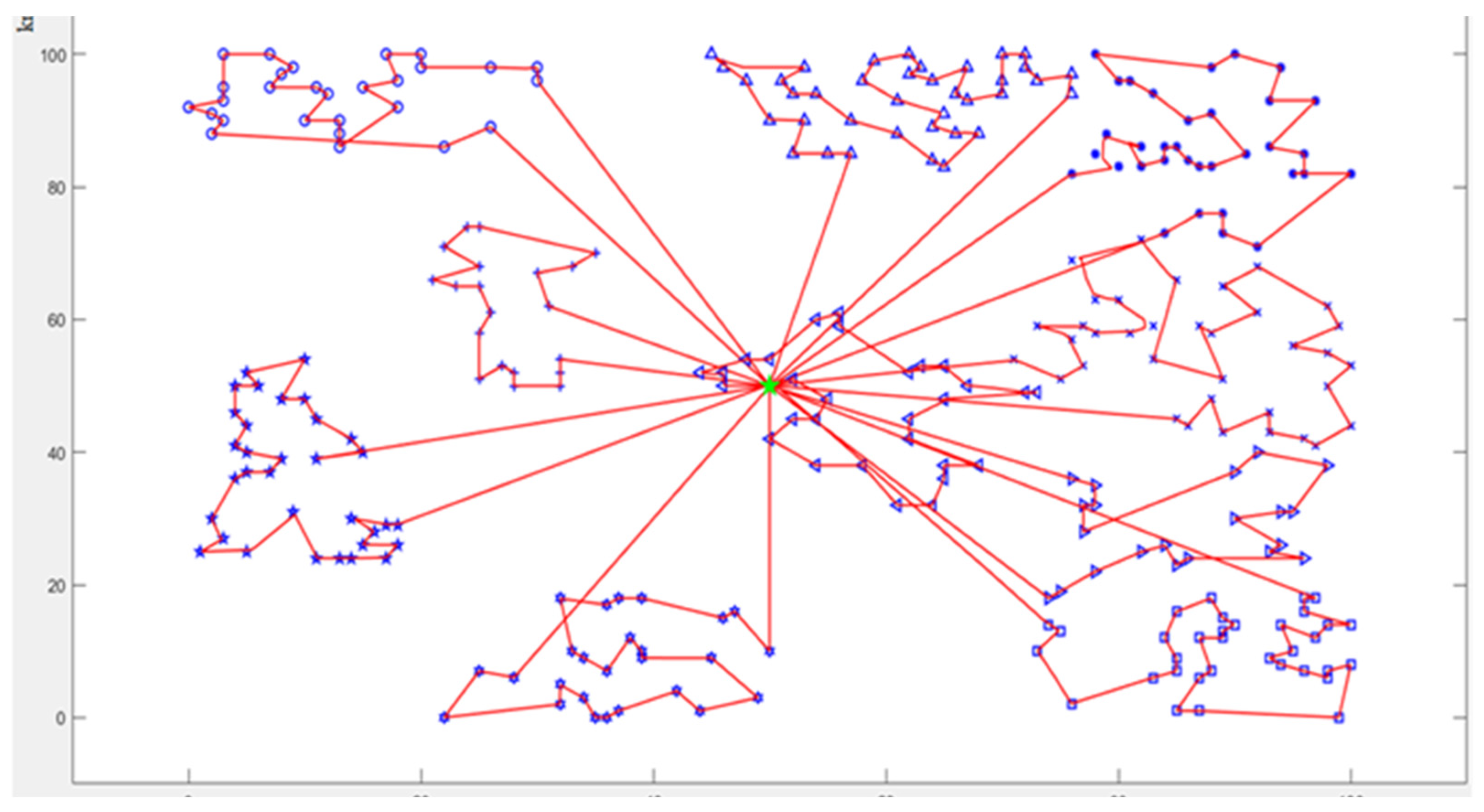
5.2.2. Partitioned Distribution Path Planning Based on Self-Organizing Map (SOM) Network

The input layer primarily receives input data, whereas the competition layer consists of a two-dimensional grid of neurons. The training process of the SOM network is divided into three principal stages: competition, cooperation, and adaptation.

(1) Competition Stage: The discrimination function in the SOM network provides the basis for competition among neurons. By calculating the input data through the discrimination function, the neuron with the highest value of the discrimination function becomes the “winner” of the competition stage. Let n represent the dimension of the input space, the input vector be denoted as $P={\left[p_1,p_2,\cdots ,p_n\right]}^T$, and the weight vector of the output neuron be denoted as

$$W_j={\left[w_{j1},w_{j2},\cdots ,w_{jn}\right]}^T,j=1,2,\cdots l,$$

(46)

where l is the number of neurons.

To obtain the optimal matching relationship between the input vector P and the synaptic weight vector $W_j$, the neuron with the maximum inner product $W_j^{T}P$ can be selected through comparison, thereby determining the position of the topological neighborhood center of the excited neuron. The expression for the winner $i\left(P\right)$ is

$$i\left(P\right)=\arg \min ‖P-W_j‖,j=1,2,\cdots l.$$

(47)

(2) Cooperation Stage: Neurons within the topological neighborhood centered around the winning neuron $i\left(P\right)$ are referred to as cooperating neurons. There exists an “inhibition” effect among neurons; the farther a neuron is from the winning neuron $i\left(P\right)$, the stronger the inhibition it experiences, and the closer it is, the weaker the inhibition. Let $h_{j,i}$ represent the topological neighborhood centered around the winning neuron i, and $d_{i,j}$ represent the lateral distance between the winning neuron i and the excited neuron j. The expression is given by

$$d_{i,j}=\sqrt{{\left(x_i-x_j\right)}^2+{\left(y_i-y_j\right)}^2},$$

(48)

where $x_i$ and $x_j$, $y_i$ and $y_j$ represent the x-coordinates and y-coordinates of the winning neuron and the excited neuron, respectively.

While searching for the topological neighborhood, a filter is automatically generated to update the Gaussian distribution of the winning neuron. Suppose the topological neighborhood $h_{j,i}$ is a unimodal function of the lateral distance $d_{i,j}$. The function $h_{j,i}$ must satisfy the following conditions:

(1)

The maximum value of the topological neighborhood $h_{j,i}$ defined at $d_{i,j}=0$ is symmetric, ensuring that the winning neuron i reaches its maximum at $d_{i,j}=0$.

(2)

The magnitude of the topological neighborhood $h_{j,i}$ monotonically decreases as $d_{i,j}$ increases, and $\underset{d_{i,j}\to +\mathrm{\infty }}{\lim }{h}_{j,i}=0$, satisfying the convergence condition of the SOM network.

The Gaussian function $h_{j,i}$ that meets the above two conditions is expressed as follows:

$$h_{j,i}\left(P\right)=\exp \left(-{\displaystyle \frac{d_{j,i}^2}{2{\sigma }^2}}\right).$$

(49)

To ensure that the topological neighborhood decreases with the increase in time t, the width $\mathsf{\sigma }$ of the topological neighborhood function $h_{j,i}$ can be transformed into a time-dependent function:

$$\sigma \left(t\right)={\sigma }_0\exp \left(-{\displaystyle \frac{t}{{\tau }_1}}\right),t=0,1,2\cdots ,$$

(50)

where ${\sigma }_0$ is the initial value of the width $\mathsf{\sigma }$, and ${\tau }_1$ is the time constant.

The time-dependent formulation of the topological neighborhood function $h_{j,i}$ is presented as follows:

$$h_{j,i\left(P\right)}\left(t\right)=\exp \left(-{\displaystyle \frac{d_{j,i}^2}{2{\sigma }^2\left(t\right)}}\right),t=0,1,2\cdots$$

(51)

(3) Adaptive process. The synaptic weight vector $W_j$ of neuron j in the SOM network adjusts with changes in the input vector P, thus exhibiting self-organizing and adaptive characteristics. To ensure the convergence of this model, a learning rate $\eta$ is introduced in this chapter to control the iterative convergence of the algorithm. By setting a scalar function $\mathrm{g}\left(y_i\right)$, the weight vector can be transformed into

$$\Delta W_j=\eta y_{j}P-g\left(y_j\right)W_j.$$

(52)

The function $\mathrm{g}\left(y_i\right)$ can be chosen as a linear function:

$$g\left(y_j\right)=\eta y_j,$$

(53)

$$y_j=h_{j,i\left(P\right)},$$

(54)

transforming Equation (54) into

$$\Delta W_j=\eta h_{j,i\left(P\right)}\left(P-W_j\right).$$

(55)

Let the weight vector of neuron j at time t be $W_j\left(t\right)$. Then, the updated weight vector $W_j(t+1)$ at time $t+1$ is defined as

$$W_j\left(t+1\right)=W_j\left(t\right)+\eta \left(t\right)h_{j,i\left(P\right)}\left(t\right)\left(P-W_j\left(t\right)\right).$$

(56)

In the above equation, the learning rate $\eta$ is represented as a time function $\eta \left(t\right)$, which should start from an initial value $\eta$₀ and decrease as time t increases. $\eta \left(t\right)$ can be expressed as

$$\eta \left(t\right)={\eta }_0\exp \left(-{\displaystyle \frac{t}{{\tau }_2}}\right),t=0,1,2\cdots ,$$

(57)

where ${\tau }_2$ is the time constant.

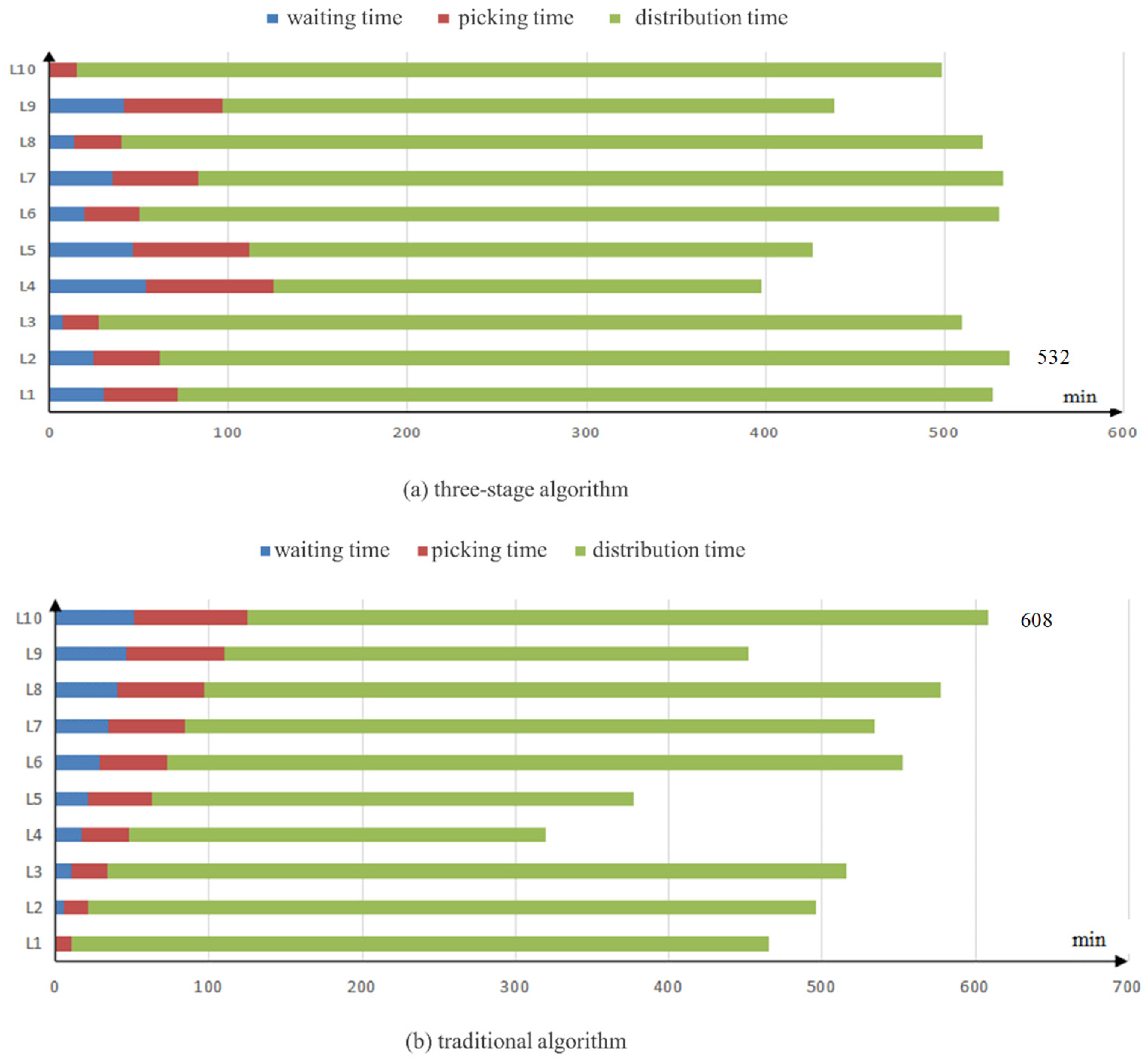
5.2.3. Autonomous Adjustment of Order Batch Picking Based on Distribution Duration

Customer orders are clustered according to their order areas, and the picking sequence of orders on each route is arranged according to the required distribution time for each area. Routes requiring longer distribution times receive higher priority for order picking. Furthermore, orders are batched for picking according to the storage locations of their contained goods. This approach minimizes distribution vehicle waiting times during picking operations, thereby enhancing the overall efficiency of integrated picking and distribution.

The flowchart of the three-stage algorithm for joint scheduling of picking and distribution is shown in Figure 5.

6. Case Study

6.1. Storage Location Allocation of Inbound Operation

Taking the storage location planning of an industrial goods storage area as an example, the proposed algorithm in this paper is verified. The centers of the goods are all labeled with white RFID tags, and fixed RFID readers are installed at specific positions on the stacker crane to identify goods labels. RFID tags are also fixed to storage locations in designated areas to monitor the occupancy status of storage slots in real time. The conveyor speed is $v_{h1}$ = 1 m/s, the stacker crane’s horizontal movement speed is $v_{h2}$ = 1.6 m/s, and its vertical movement speed is $v_v$ = 0.6 m/s. The unit storage slot size is 1.5 m × 1.5 m × 1.6 m, and each row of shelves has a specification of 10 × 5. The actual storage area of Warehouse 4.0 is divided into multi-level shelving storage zones based on the volume of the goods, i.e., the specifications of the goods boxes. Taking a shelving unit of uniform volume as an example, six rows of shelves are considered, with a total storage capacity of 6 × 10 × 5 = 300 locations. An equal weight consideration is given to picking time and shelf stability, i.e., ${\theta }_1$ = ${\theta }_2$ = 0.5. A total of 18 types of components are randomly selected from inbound orders for verification.

To validate the established storage location allocation model and the designed IMA algorithm, 18 vacant storage location coordinates are selected for the simulation. For the MA, the parameter ranges are as follows: the population size ranges from 20 to 50, the number of iterations ranges from 200 to 1000, the wedding dance coefficient ranges from 0.1 to 0.3, the wedding dance decay parameter ranges from 0.8 to 0.99, the population learning coefficient ranges from 1.5 to 2.0, the individual learning coefficient is set to 1, the visibility coefficient is 2, the mutation rate ranges from 0.01 to 0.1, the random flight coefficient ranges from 0.1 to 0.3, and the random flight decay parameter ranges from 0.8 to 0.99. Initial parameters are selected based on these ranges, and through continuous adjustment of various parameters, the results of inbound storage location allocation are optimized. For the GA, the parameter ranges are as follows: the population size ranges from 20 to 50, the number of iterations ranges from 200 to 1000, the crossover probability ranges from 0.4 to 0.9, and the mutation probability ranges from 0.01 to 0.1. The parameter tuning process for the genetic algorithm is similar to that of the MA. For the PSO, the parameter ranges are as follows: the population size ranges from 20 to 50, the number of iterations ranges from 200 to 1000, the inertia weight ranges from 0.4 to 0.9, the cognitive learning factor (c1) ranges from 1.3 to 2, and the social learning factor (c2) ranges from 1.3 to 2. The parameter tuning process for the PSO algorithm is similar to that of the MA. For the mayfly algorithm and IMA algorithm, the parameters are shown in

Table 3. Parameter selection values of the mayfly algorithm.

Parameters	Offspring	Male	Female	Iterations
Value	50	25	25	500
Parameter	Wedding Dance Coefficient	Wedding Dance Decay Parameter	Population Learning Coefficient	Individual Learning Coefficient
Value	0.1	0.8	1.5	1
Parameter	Visibility Coefficient	Mutation Rate	Random Flight Coefficient	Random Flight Decay Parameter
Value	2	0.01	0.1	0.99

. In the genetic algorithm, the population size is set to 200, the crossover rate is set to 0.85, and the mutation rate is set to 0.02; in the particle swarm optimization algorithm, the number of particles is set to 50, ω (inertia weight) is set to 0.6, and c₁ = c₂ = 1.4 (acceleration coefficients). It should be noted that the initial parameter values for these algorithms were determined based on a comprehensive review of the relevant literature as well as preliminary experimental results. All experiments are conducted on a hardware platform equipped with an Intel (Santa Clara, CA, USA) i5-7300HQ processor, a GTX1050-8G graphics card, and 12 GB RAM. The software testing environment is MATLAB R2020a. Figure 6 illustrates the impact of various parameters of the IMA on the experimental results. Figure 7 shows a comparison of the fitness value curves with the number of iterations.

Table 4. The values of the parameters for different algorithms.

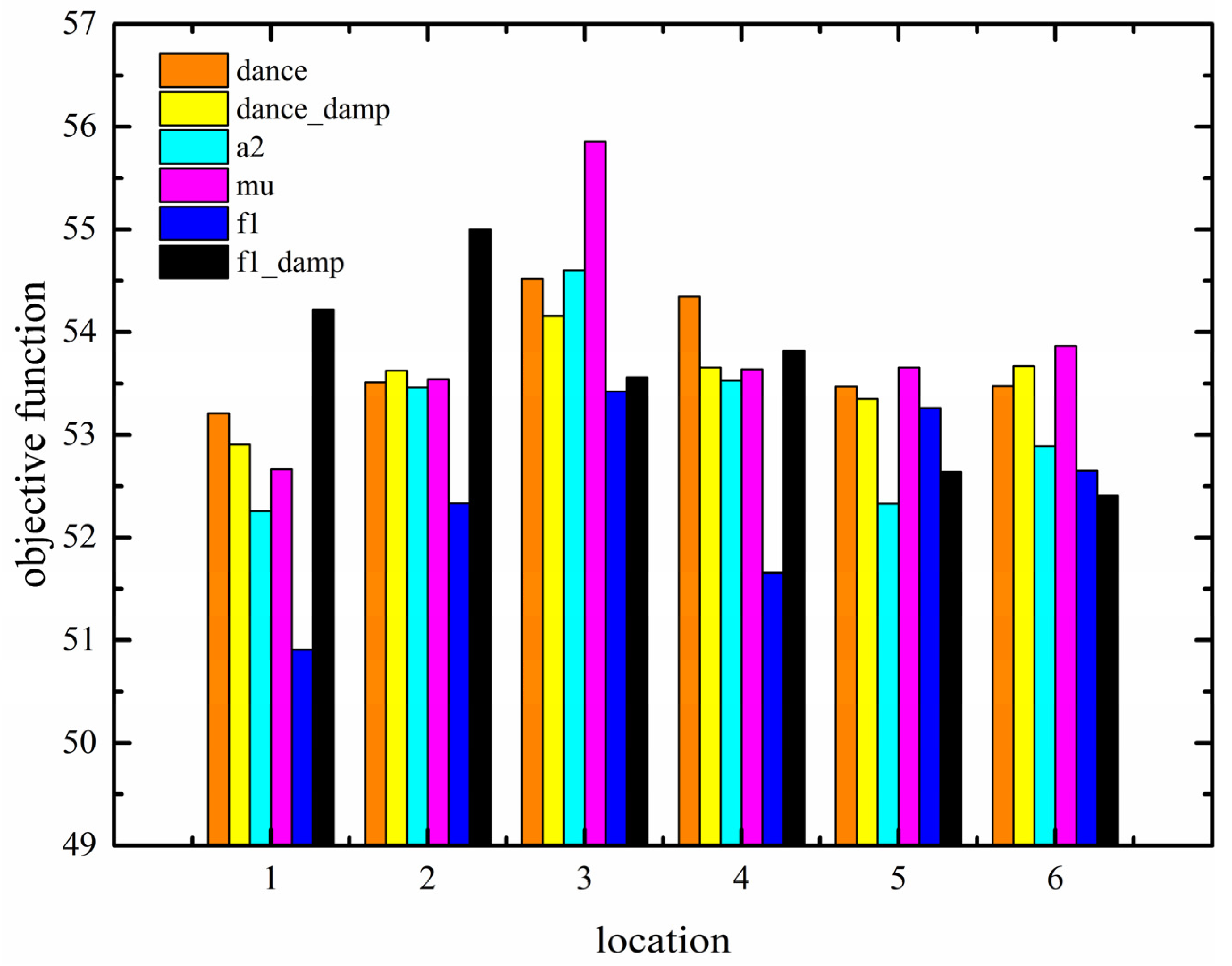
Location	1	2	3	4	5	6
Parameter
pc	0.45	0.55	0.65	0.75	0.85	0.95
pm	0.01	0.02	0.04	0.06	0.08	0.10
w	0.40	0.50	0.60	0.70	0.80	0.90
c1	1.30	1.40	1.50	1.60	1.70	1.80
c2	1.30	1.40	1.50	1.60	1.70	1.80
dance	0.10	0.14	0.18	0.22	0.26	0.30
dance_damp	0.80	0.84	0.88	0.92	0.96	0.99
a2	1.50	1.60	1.70	1.80	1.90	2.00
mu	0.01	0.03	0.05	0.07	0.09	0.10
f1	0.10	0.14	0.18	0.22	0.26	0.30
fl_damp	0.80	0.84	0.88	0.92	0.96	0.99

presents the values of the parameters for different algorithms.

Table 5. IMA-based allocation results of vacant storage locations for inbound order items.

ID	Shipper Name	Goods Name	Container Specifications	Shipper Level	Weight (kg)	Storage Period (Days)	Turnover Rate	Allocated Storage Location
1	A1	Deep Groove Ball Bearing	5	1	15	30	0.24	(2, 2, 3)
2	B1	Cylindrical Gear	5	2	10	35	0.32	(1, 2, 4)
3	A3	M10 Bolt	4	1	70	40	0.15	(4, 1, 3)
4	C1	Gear Coupling	1	3	100	10	0.5	(1, 4, 1)
5	B2	Worm Gear	3	2	80	360	0.52	(3, 2, 1)
6	B2	Jaw Clutch	4	2	25	120	0.19	(3, 1, 4)
7	B2	V-Belt	4	2	30	90	0.23	(2, 1, 2)
8	B2	Chain	3	2	5	90	0.12	(4, 4, 4)
9	A2	M20 Bolt	5	1	35	90	0.42	(2, 5, 1)
10	A2	Double-Ended Stud	3	1	10	90	0.82	(2, 2, 4)
11	A2	Lock Nut	2	1	28	120	0.32	(3, 2, 2)
12	A1	Washer	5	1	10	150	0.54	(3, 1, 3)
13	A1	Spring	5	1	26	150	0.2	(4, 3, 3)
14	A1	Helical Gear	4	1	60	90	0.28	(3, 1, 2)
15	A1	Bevel Gear	1	1	50	90	0.74	(1, 1, 1)
16	A1	Spur Gear	1	1	22	100	0.74	(1, 2, 2)
17	A1	Herringbone Gear	1	1	30	60	0.74	(1, 3, 1)
18	A1	Overflow Valve	1	1	30	100	0.74	(2, 3, 1)

presents the results of the IMA algorithm for the allocation of vacant storage locations to inbound order goods.

To analyze the effectiveness of the IMA algorithm, a comparative analysis is conducted, and the calculation results are shown in

Table 6. Comparison of calculation results of various algorithms.

Algorithm	Best		Worst		Average
	Fitness Value	Convergence Count	Fitness Value	Convergence Count	Fitness Value	Convergence Count
IMA	45.98	18	53.95	286	48.11	109
MA	59.46	385	61.56	450	60.23	428
PSO	60.79	280	64.13	422	62.73	307
GA	61.86	291	65.32	356	63.86	316

. Meanwhile, the time complexity of the algorithms is compared, and the results are shown in

Table 7. Comparison of the time complexity of various algorithms.

Algorithm	Theoretical Complexity	Measured Time (n = 1000)
IMA	O(mn)	8 s
MA	O(mn logn)	14 s
PSO	O(m2n)	10 s
GA	O(mn2)	12 s

.

From Table 6, it is evident that in terms of convergence speed, the IMA converges 64.5%, 65.5%, and 74.5% faster than PSO, GA, and MA, respectively. In terms of fitness value, the IMA achieves a fitness value that is 23.3%, 24.7%, and 20.1% lower than that of PSO, GA, and MA, respectively. From Table 7, in terms of speedup ratio, the IMA is 20%, 29%, and 39% faster than the PSO, GA, and MA, respectively. This demonstrates that the IMA designed in this paper is superior to MA, GA, and PSO in both obtaining the optimal value and the number of convergence iterations.

6.2. Joint Scheduling of Picking and Distribution for Outbound Operation

Due to the characteristics of small batch sizes and high frequency, the quantity of goods required for each customer order follows a uniform distribution in the range of [1, 5]. The picking area setup and stacker crane parameters are as follows: the shelving unit has 6 rows, 12 columns, and 15 layers, with a horizontal speed $v_h$ = 1.5 m, vertical speed $v_v$ = 0.6 m, and length L = 1.5 m. The coordinates of the distribution customers are randomly distributed on a two-dimensional map within a range of 100 km × 100 km, and the coordinates of the distribution center are (50 km, 50 km). The distribution vehicle speed $v_l$ is set to 40 km/h, and the service time T for each customer is set to 5 min. After multiple simulations, the parameters for the GMM and SOM algorithms are set as follows: in the GMM, the maximum loading capacity $Q_l$ of the truck is set to 100, and the convergence function LL(D) threshold is 10⁻². In the SOM, the maximum number of iterations is set to 1000, and the number of neurons $M_i$ is set to 4 times the number of samples in each category. The hardware environment for algorithm operation consists of an Intel (Santa Clara, CA, USA) i5-7300HQ processor, GTX1050-8G GPU, and 12 GB memory, and the software environment for algorithm operation comprises MatlabR2020a.

As shown in Figure 8, considering the vehicle’s load capacity, the improved GMM clustering algorithm divides the 300 customer locations in the case into 10 distribution areas. The number of goods required to be delivered by vehicles responsible for each area is as follows: first category 100 units; second category 100 units; third category 97 units; fourth category 94 units; fifth category 99 units; sixth category 99 units; seventh category 100 units; eighth category 100 units; ninth category 94 units; and tenth category 96 units. The horizontal and vertical coordinates in the figure represent the geographical location coordinates of the customers on the map.

The 10 distribution routes calculated are shown in Figure 9. The distribution times for each route, L1~L10, are 455 min, 475 min, 482 min, 272 min, 314 min, 480 min, 450 min, 481 min, 342 min, and 483 min, respectively.

Based on the three-stage algorithm approach and the distribution times for each area, the picking sequence for this case is determined to be L10 → L3 → L8 → L6 → L2 → L1 → L7 → L9 → L5 → L4.

Table 8. Comparison results of the three-stage algorithm and the traditional FIFO algorithm.

		Three-Stage Algorithm			Traditional FIFO Algorithm
Area	Distribution Time (min)	Picking Start Time (min)	Picking Time (min)	Distribution End Time (min)	Picking Start Time (min)	Picking Time (min)	Distribution End Time (min)
L1	455	30	41	526	0	10	465
L2	475	24	36	536	4	16	496
L3	482	7	19	509	10	23	515
L4	272	53	71	397	16	30	319
L5	314	46	65	426	21	40	376
L6	480	19	30	530	28	43	552
L7	450	35	47	532	34	49	533
L8	481	13	26	520	40	56	577
L9	342	41	55	438	46	64	452
L10	483	0	15	498	51	73	608
Fulfillment Time		536			608
Average Fulfillment Time		491			500

compares the three-stage algorithm with the traditional First-In-First-Out (FIFO) algorithm in this scenario, showing the distribution time, picking start time, picking time, and distribution end time for each route. The execution time for the three-stage algorithm is 536 min, while the execution time for the traditional FIFO algorithm is 608 min.

Figure 10 shows the Gantt charts for the picking and distribution of each area using the three-stage algorithm and the FIFO algorithm, respectively.

From Figure 9, it can be seen that, compared to the traditional FIFO algorithm, the three-stage algorithm shortens the order fulfillment time by 12% and reduces the average fulfillment time by 1.8%. It is evident that integrating the scheduling of distribution and picking operations helps in improving the overall distribution efficiency of the warehouse, enhancing customer satisfaction, and improving the utilization rate of distribution resources and vehicles.

7. Conclusions

This paper proposes an integrated implementation framework for Warehouse 4.0, which uses automation, IoT, and big data technologies to build an intelligent warehousing system. It solves the inbound and outbound operations in Warehouse 4.0 through swarm intelligence and coordinated scheduling strategies.

(1)

An improved mayfly algorithm (IMA) incorporating adaptive dynamic inertia weight factors, Lévy flight strategies, and golden sine factors is developed for parallel stacker crane scenarios. Simulations demonstrate that IMA achieves 64.5%, 65.5%, and 74.5% faster convergence speeds compared to PSO, GA, and MA, respectively, with fitness values reduced by 23.3%, 24.7%, and 20.1%.

(2)

A three-stage algorithm integrates Gaussian clustering for customer analysis, self-organizing neural networks for route planning, and operation-duration-based picking sequence optimization. Case studies verify a 12% reduction in order fulfillment time and a 1.8% improvement in average processing efficiency compared to traditional FIFO methods.

A key limitation of the current work is that, during the clustering decision analysis of outbound orders, the scheduling decision scheme primarily considers the customer’s location and the maximum capacity of the distribution vehicle, without taking the customer’s distribution time requirements into account. Future work will involve considering the customer’s distribution time constraints to further enhance customer satisfaction and improve the overall efficiency of warehousing logistics operations.

References

- Leng, J.W.; Jiang, P.Y.; Xu, K.L.; Liu, Q.; Zhao, J.L.; Bian, Y.Y.; Shi, R. Makerchain: A Blockchain with Chemical Signature for Self-Organizing Process in Social Manufacturing. J. Clean. Prod. 2019, 234, 767–778. [Google Scholar] [CrossRef]
- Tubis, A.A.; Rohman, J. Intelligent Warehouse in Industry 4.0-Systematic Literature Review. Sensors 2023, 23, 4105. [Google Scholar] [CrossRef] [PubMed]
- Guo, J.L.; Leng, J.W.; Zhao, L.; Zhou, X.L.; Yuan, Y.; Lu, Y.Q.; Mourtzis, D.; Qi, Q.L.; Huang, S.H.; Song, X.G.; et al. Industrial metaverse towards Industry 5.0: Connotation, architecture, enablers, and challenges. J. Manuf. Syst. 2024, 76, 25–42. [Google Scholar] [CrossRef]
- Leng, J.W.; Zhou, M.; Xiao, Y.X.; Zhang, H.; Liu, Q.; Shen, W.M.; Su, Q.Y.; Li, L.Z. Digital Twins-based Remote Semi-Physical Commissioning of Flow-Type Smart Manufacturing Systems. J. Clean. Prod. 2021, 306, 127278. [Google Scholar] [CrossRef]
- Leng, J.W.; Guo, J.W.; Xie, J.X.; Zhou, X.L.; Liu, A.; Gu, X.; Mourtzis, D.; Qi, Q.L.; Liu, Q.; Shen, W.M.; et al. Review of manufacturing system design in the interplay of Industry 4.0 and Industry 5.0 (Part I): Design thinking and modeling methods. J. Manuf. Syst. 2024, 76, 158–187. [Google Scholar] [CrossRef]
- Leng, J.W.; Zhong, Y.W.; Lin, Z.S.; Xu, K.L.; Mourtzis, D.; Zhou, X.L.; Zheng, P.; Liu, Q.; Zhao, J.L.; Shen, W.M. Towards resilience in Industry 5.0: A decentralized autonomous manufacturing paradigm. J. Manuf. Syst. 2023, 71, 95–114. [Google Scholar] [CrossRef]
- Leng, J.W.; Sha, W.N.; Lin, Z.S.; Jing, J.B.; Liu, Q.; Chen, X. Blockchained smart contract pyramid-driven multi-agent autonomous process control for resilient individualised manufacturing towards Industry 5.0. Int. J. Prod. Res. 2023, 61, 4302–4321. [Google Scholar] [CrossRef]
- Tsou, M.C. Online analysis process on Automatic Identification System data warehouse for application in vessel traffic service. Proc. Inst. Mech. Eng. Part M-J. Eng. Marit. Environ. 2016, 230, 199–215. [Google Scholar] [CrossRef]
- Liu, J.M.; Liao, H.T.; White, J.A. Stochastic analysis of an automated storage and retrieval system with multiple in-the-aisle pick positions. Nav. Res. Logist. 2021, 68, 454–470. [Google Scholar] [CrossRef]
- Shoaee, M.; Samouei, P. Clusters of floor locations-allocation of stores to cross-docking warehouse considering satisfaction and space using MOGWO and NSGA-II algorithms. Flex. Serv. Manuf. J. 2024, 36, 315–342. [Google Scholar] [CrossRef]
- Wan, Y.C.; Wang, S.D.; Hu, Y.J.; Xie, Y.Y. Multiobjective Optimization of the Storage Location Allocation of a Retail E-commerce Picking Zone in a Picker-to-parts Warehouse. Eng. Lett. 2023, 31, 232023. [Google Scholar]
- Gao, J.; Xie, W.D.; Shi, D.K.; Wu, J.; Wang, R. Synchronized optimization of the logistics system of a tobacco high-bay warehouse under production task fluctuations. Eng. Res. Express. 2024, 6, 045580. [Google Scholar] [CrossRef]
- Ma, Q.L.; Xu, L.L.; Zhu, L.; Jia, P. Research on storage location allocation in three-dimensional automated warehouse based on cargo damage control. Int. J. Ind. Eng. Comput. 2025, 16, 177–196. [Google Scholar] [CrossRef]
- Islam, M.S.; Uddin, M.K. An efficient correlation-based storage location assignment heuristic for multi-block multi-aisle warehouses. Int. J. Ind. Eng. Manag. 2024, 15, 125–139. [Google Scholar] [CrossRef]
- Rungjaroenporn, C.; Setthawong, R. Multiobjective Optimization Using Flower Pollination Algorithm for Storage Location Assignment at Lazada Thailand Warehouse. In Proceedings of the 13th International Conference on Knowledge and Smart Technology (KST), Bangsaen, Thailand, 21–24 January 2021. [Google Scholar]
- Xu, X.B.; Ren, C.H. Research on Dynamic Storage Location Assignment of Picker-to-Parts Picking Systems under Traversing Routing Method. Complexity 2020, 2020, 1621828. [Google Scholar] [CrossRef]
- Zhang, S.W.; Fu, L.P.; Chen, R.; Mei, Y. Optimizing the Cargo Location Assignment of Retail E-Commerce Based on an Artificial Fish Swarm Algorithm. Math. Probl. Eng. 2020, 2020, 1621828. [Google Scholar] [CrossRef]
- De Puiseau, C.W.; Nanfack, D.T.; Tercan, H.; Löbbert-Plattfaut, J.; Meisen, T. Dynamic Storage Location Assignment in Warehouses Using Deep Reinforcement Learning. Technologies 2023, 10, 129. [Google Scholar] [CrossRef]
- Leng, J.W.; Yan, D.X.; Liu, Q.; Zhang, H.; Zhao, G.G.; Wei, L.J.; Zhang, D.; Yu, A.L.; Chen, X. Digital twin-driven joint optimisation of packing and storage assignment in large-scale automated high-rise warehouse product-service system. Int. J. Comput. Integr. Manuf. 2021, 34, 783–800. [Google Scholar] [CrossRef]
- Gao, S.; Qi, L.; Lei, L. Integrated batch production and distribution scheduling with limited vehicle capacity. Int. J. Prod. Econ. 2015, 160, 13–25. [Google Scholar] [CrossRef]
- Li, K.; Zhou, C.; Leung, J.Y.T.; Ma, Y. Integrated production and delivery with single machine and multiple vehicles. Expert Syst. Appl. 2016, 57, 12–20. [Google Scholar] [CrossRef]
- Rasti-Barzoki, M.; Hejazi, S.R. Pseudo-polynomial dynamic programming for an integrated due date assignment, resource allocation, production, and distribution scheduling model in supply chain scheduling. Appl. Math. Model. 2015, 39, 3280–3289. [Google Scholar] [CrossRef]
- Suppini, C.; Lysova, N.; Bocelli, M.; Solari, F.; Tebaldi, L.; Volpi, A.; Montanari, R. From Single Orders to Batches: A Sensitivity Analysis of Warehouse Picking Efficiency. Sustainability 2024, 16, 8231. [Google Scholar] [CrossRef]
- Schumann, D.; Cevirgen, C.; Becker, J.; Arian, O.; Nyhuis, P. Development of a Procedure Model to Compare the Picking Performance of Different Layouts in a Distribution Center. In Proceedings of the 8th International Conference on Competitive Manufacturing (COMA), Stellenbosch, South Africa, 9–11 March 2022. [Google Scholar]
- Modenov, A.; Boboshko, A.; Durandina, A.; Kharchenko, O. A New Mathematical Model for Joint Production and Distribution Optimization in a Multi-Echelon Supply Chain. Ind. Eng. Manag. Syst. 2021, 20, 349–355. [Google Scholar] [CrossRef]
- Han, D.Y.; Yang, Y.J.; Wang, D.J.; Cheng, T.C.E.; Yin, Y.Q. Integrated production, inventory, and outbound distribution operations with fixed departure times in a three-stage supply chain. Transp. Res. Part E-Logist. Transp. Rev. 2019, 125, 334–347. [Google Scholar] [CrossRef]
- Czerniachowska, K.; Wichniarek, R.; Zywicki, K. Matheuristics for the Order-picking Problem with Sequence-dependant Constraints in a Logistic Center with a One-directional Conveyor Between Buffers. Manag. Prod. Eng. Rev. 2024, 15, 140–160. [Google Scholar] [CrossRef]
- Czerniachowska, K.; Wichniarek, R.; Zywicki, K. A Model for an Order-Picking Problem with a One-Directional Conveyor and Buffer. Sustainability 2023, 15, 13731. [Google Scholar] [CrossRef]
- Tsang, Y.P.; Wu, C.H.; Lam, H.Y.; Choy, K.L.; Ho, G.T.S. Integrating Internet of Things and multi-temperature delivery planning for perishable food E-commerce logistics: A model and application. Int. J. Prod. Res. 2021, 59, 1534–1556. [Google Scholar] [CrossRef]
- Mukherjee, T.; Sangal, I.; Sarkar, B.; Alkadash, T.M.; Almaamari, Q. Pallet Distribution Affecting a Machine’s Utilization Level and Picking Time. Mathematics 2023, 11, 2956. [Google Scholar] [CrossRef]
- Zhang, F.Q.; Xu, F.L.; Zhou, X.L.; Ding, K.; Shao, S.J.; Du, C.; Leng, J.W. Data-driven and Knowledge-guided Prediction Model of Milling Tool Life Grade. Int. J. Comput. Integr. Manuf. 2024, 37, 669–684. [Google Scholar] [CrossRef]