
Unveiling Hidden Dynamics in Air Traffic Networks: An Additional-Symmetry-Inspired Framework for Flight Delay Prediction


Abstract
1. Introduction
2. Theoretical Background: DenseNet-LSTM-FBLS
2.1. Fuzzy Broad Learning System (FBLS)
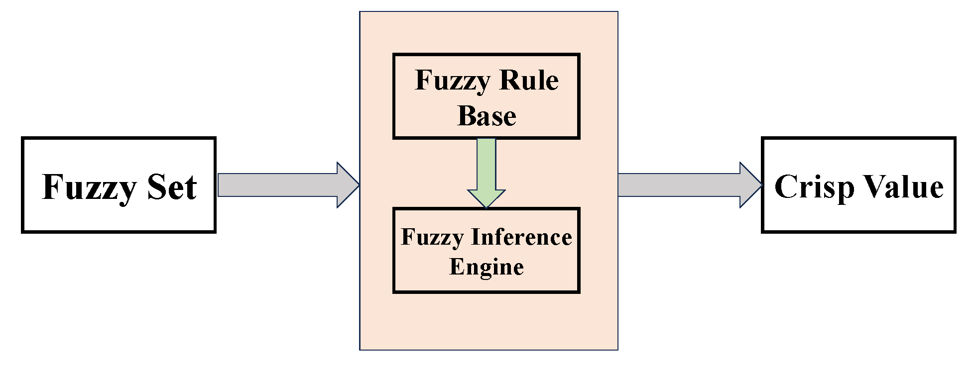
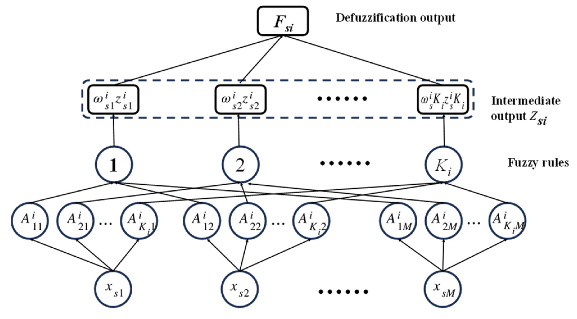
2.1.1. TSK Fuzzy System
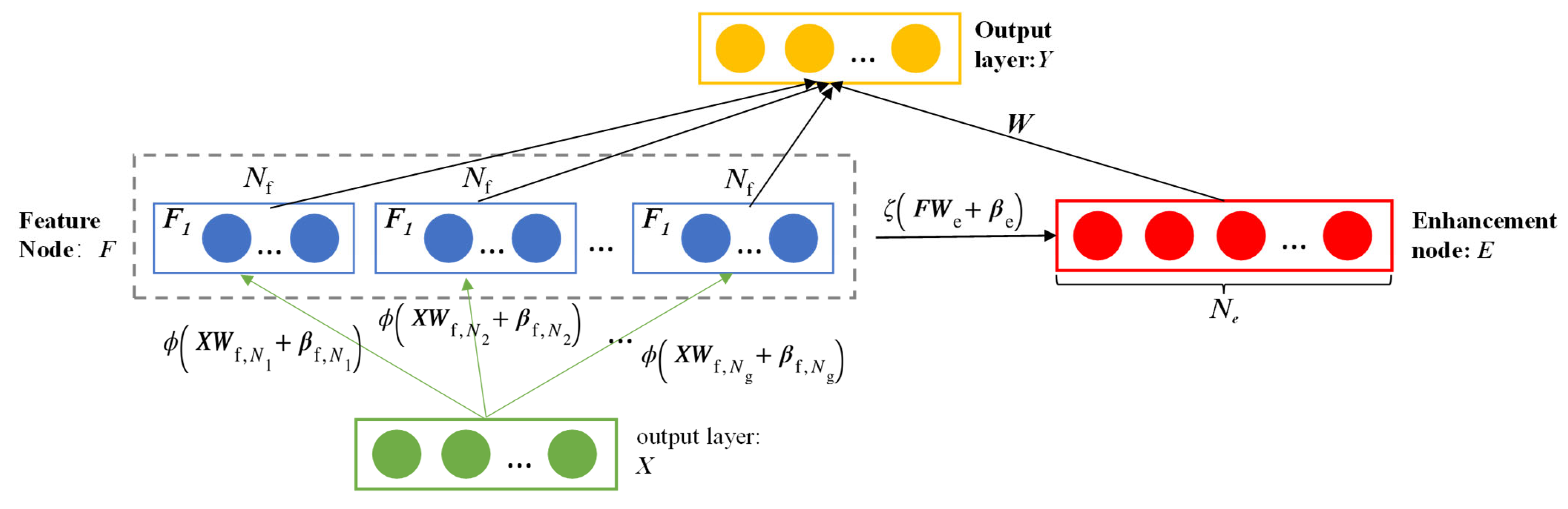
2.1.2. Broad Learning System (BLS)
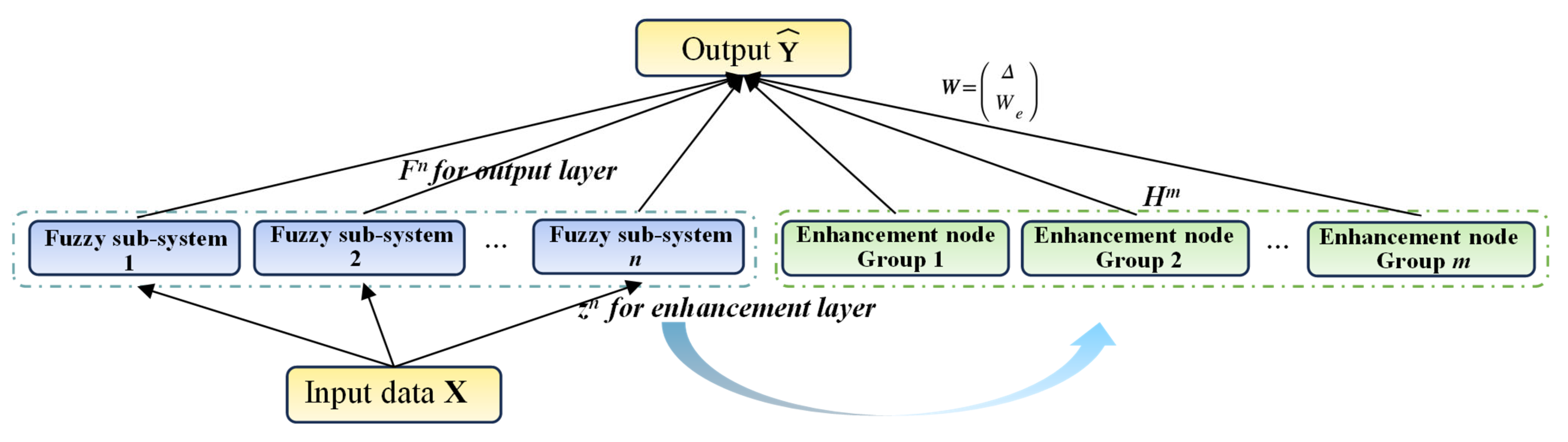
2.1.3. FBLS
2.1.4. Algorithm Flow
| Algorithm 1. FBLS Training Algorithm |
| Input: Training samples (X,Y) ∈RN×(M+C), numbers of fuzzy rules Ki, enhancement nodes Lj, fuzzy subsystems n and enhancement node groups m. |
| Output: Training time T1, and maximum allowed training time |
| 1. Set a standard deviation of 1, which will be used to calculate the parameters of the fuzzy subsystem function. |
| 2. Start the timer to measure the code execution time. |
| 3. Standardize the training data. |
| 4. Define a vector to store information about the training data, where the vector consists of all fuzzy rules from the i-th fuzzy subsystem. |
| 5. Store the training data in the predefined vector. |
| 6. Create a zero matrix y, which will be used to store the fuzzy outputs. |
| 7. Begin a loop, with the number of iterations determined by the number of fuzzy rules in the input variable, aimed at searching for the optimal number of fuzzy systems. |
| 8. Perform the fuzzy subsystem design, including the layout of the fuzzy system |
| 9. Use the K-means algorithm to cluster the training data and obtain the cluster centers. |
| 10. Calculate the fuzzy rules and the membership functions according to the predefined settings of the fuzzy subsystems. |
| 11. Apply standardization to the membership functions, ensuring they are in the range [0, 1]. |
| 12. Use the output of the system T1 and the corresponding feature values to calculate the final hierarchical output. |
| 13. Use the pseudoinverse to calculate the final weight matrix and apply the Jacobian matrix to derive the final output Y |
| 14. Continue this process by optimizing the system’s structure to minimize the error. |
| 15. Calculate the difference between the current output and the target output from the previous iteration. If the difference is less than the threshold, stop the training. |
| 16. Output the final model’s accuracy and training time. |
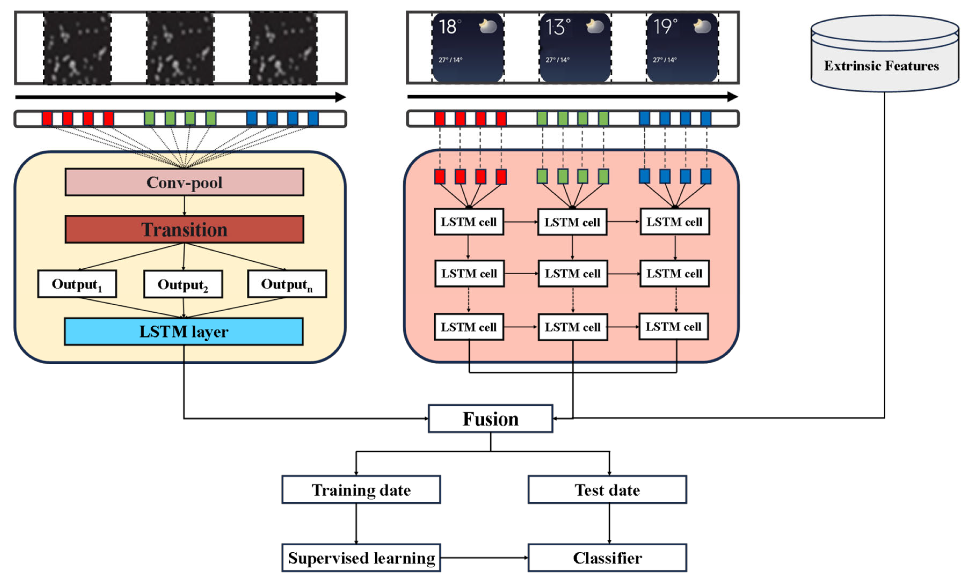
2.2. DenseNet-LSTM
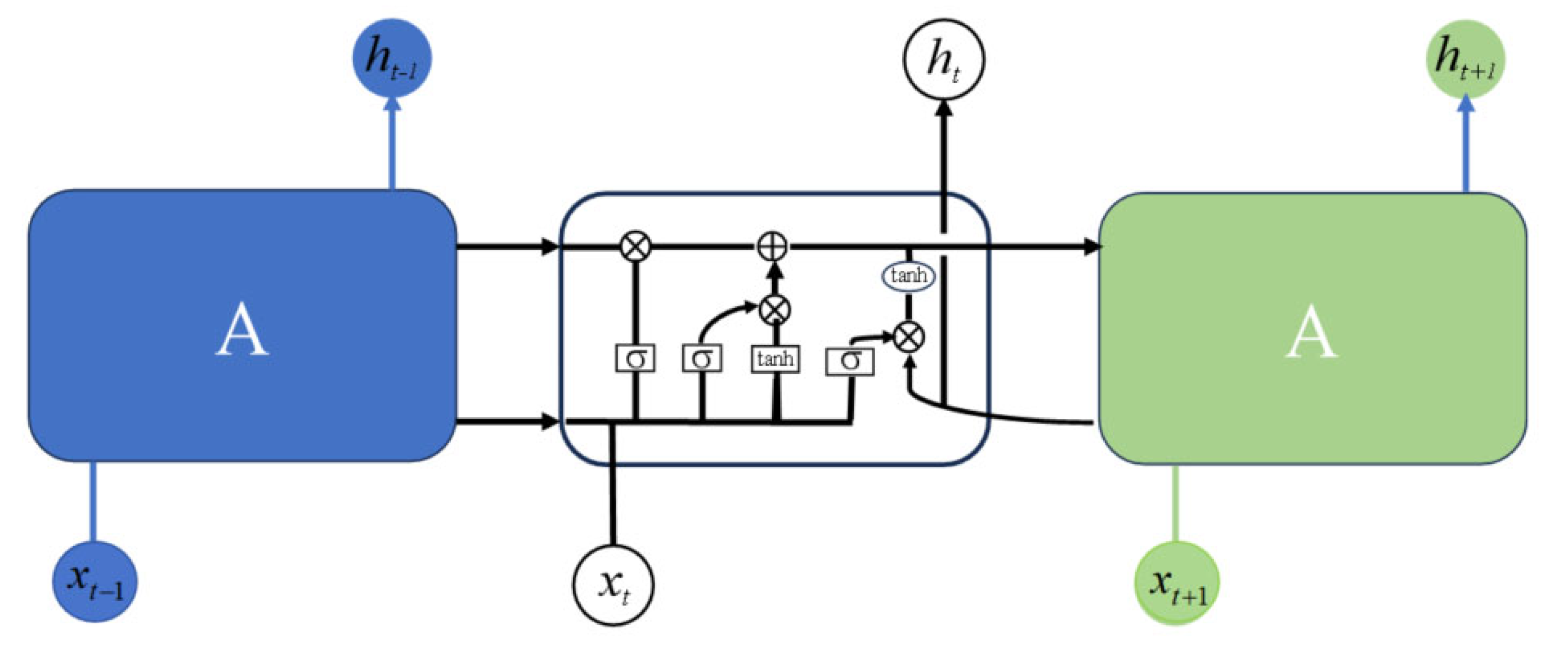
2.2.1. Temporal Feature Extraction
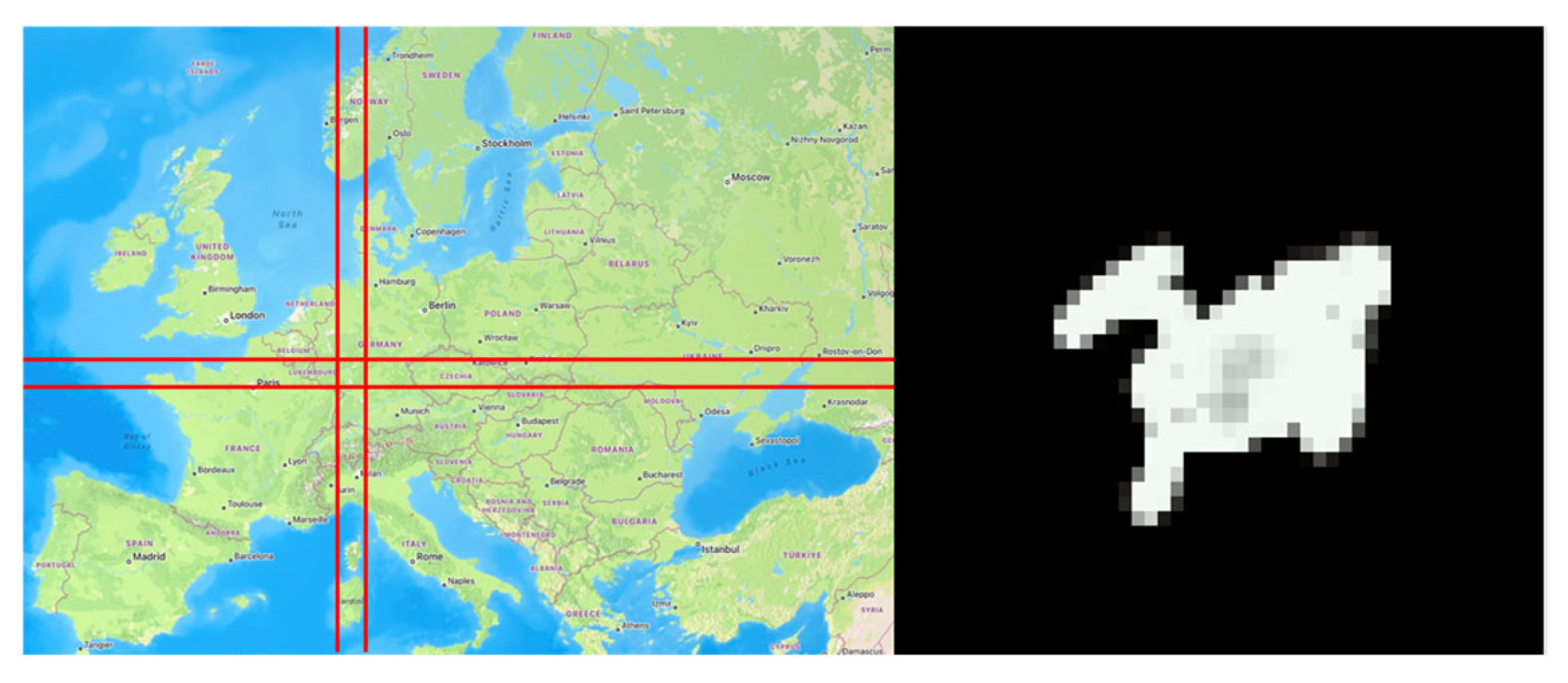
2.2.2. Method for Extracting Spatial Correlations Using DenseNet
2.2.3. Training of the DenseNet-LSTM-FBLS Model
| Algorithm 2: DenseNet-LSTM-FBLS for Flight Delay Prediction |
| Input: D: {d1, d2, …, dm, Y}, dataset containing flight data Iw: time-series data of weather attributes {Wt, W{t-1}, …, W{t-n}} Ist: time-series data of flight delays and airport congestion XExt: external features {x1, x2, …, xn} |
| Output: The class of flight delays (on-time or delay) |
| For i in range(epochs) do |
| N = spatial feature information |
| For attribute value Ist in Ist do |
| N = FDenseNet(Ist) |
| N += N |
| end |
| T = temporal feature information |
| T = FLSTM(Iw) |
| ALL = N + T + XExt |
| Ŷ = FFBLS(ALL) |
| params_grad = evaluate_gradient (loss_function = (Ŷ − Y)^2) |
| Update_model(params_grad) |
| end |
| Ypred = FFBLS*predict(ALL, Y) |
3. Experimental Results
3.1. Experimental Environment
3.2. Data and Processing
3.2.1. Source of Data
3.2.2. Data Preprocessing
- Missing value handling
- feature code
3.2.3. Imbalance Handling
3.3. Experimental Setup
3.3.1. Parameter Settings
3.3.2. Evaluation Indicators
3.4. Projected Results
3.5. Experimental Results and Analysis
4. Conclusions
Author Contributions
Funding
Data Availability Statement
Conflicts of Interest
References
- Bisandu, D.B.; Moulitsas, I. Prediction of flight delay using deep operator network with gradient-mayfly optimisation algorithm. Expert Syst. Appl. 2024, 247, 123306. [Google Scholar] [CrossRef]
- Zeng, L.; Wang, B.; Wang, T.; Wang, Z. Research on delay propagation mechanism of air traffic control system based on causal inference. Transp. Res. Part C Emerg. Technol. 2022, 138, 103622. [Google Scholar] [CrossRef]
- Ma, R.; Huang, A.; Jiang, Z.; Luo, Q.; Zhang, X. A data-driven optimal method for massive passenger flow evacuation at airports under large-scale flight delays. Reliab. Eng. Syst. Saf. 2024, 245, 109988. [Google Scholar] [CrossRef]
- Maksudova, Z.; Shakurova, L.; Kustova, E. Simulation of Shock Waves in Methane: A Self-Consistent Continuum Approach Enhanced Using Machine Learning. Mathematics 2024, 12, 2924. [Google Scholar] [CrossRef]
- Mokhtarimousavi, S.; Mehrabi, A. Flight delay causality: Machine learning technique in conjunction with random parameter statistical analysis. Int. J. Transp. Sci. Technol. 2023, 12, 230–244. [Google Scholar] [CrossRef]
- Qu, J.; Wu, S.; Zhang, J. Flight Delay Propagation Prediction Based on Deep Learning. Mathematics 2023, 11, 494. [Google Scholar] [CrossRef]
- Khan, W.A.; Ma, H.L.; Chung, S.H.; Wen, X. Hierarchical integrated machine learning model for predicting flight departure delays and duration in series. Transp. Res. Part C Emerg. Technol. 2021, 129, 103225. [Google Scholar] [CrossRef]
- Ahmadbeygi, S.; Cohn, A.; Lapp, M. Decreasing airline delay propagation by reallocating scheduled slack. IIE Trans. 2010, 42, 478–489. [Google Scholar] [CrossRef]
- Pyrgiotis, N.; Malone, K.M.; Odoni, A. Modelling delay propagation within an airport network. Transp. Res. Part C 2013, 27, 60–75. [Google Scholar] [CrossRef]
- Baspinar, B.; Ure, N.K.; Koyuncu, E.; Inalhan, G. Analysis of delay characteristics of European air traffic through a data driven airport-centric queuing network model. IFAC-Pap. 2016, 49, 359–364. [Google Scholar] [CrossRef]
- Moreira, L.; Dantas, C.; Oliveira, L.; Soares, J.; Ogasawara, E. On Evaluating Data Preprocessing Methods for Machine Learning Models for Flight Delays. In Proceedings of the 2018 International Joint Conference on Neural Networks (IJCNN), Rio de Janeiro, Brazil, 8–13 July 2018. [Google Scholar]
- Prakash, N.; Manconi, A.; Loew, S. Mapping landslides on EO data: Performance of deep learning models vs. traditional machine learning models. Remote Sens. 2020, 12, 346. [Google Scholar] [CrossRef]
- Karypidis, E.; Mouslech, S.G.; Skoulariki, K.; Gazis, A. Comparison Analysis of Traditional Machine Learning and Deep Learning Techniques for Data and Image Classification. arXiv 2022, arXiv:2204.05983. [Google Scholar] [CrossRef]
- Yazdi, M.F.; Kamel, S.R.; Chabok, S.J.M.; Kheirabadi, M. Flight delay prediction based on deep learning and Levenberg-Marquart algorithm. J. Big Data 2020, 7, 106. [Google Scholar] [CrossRef]
- Cai, K.; Li, Y.; Fang, Y.P.; Zhu, Y. A deep learning approach for flight delay prediction through time-evolving graphs. IEEE Trans. Intell. Transp. Syst. 2021, 23, 11397–11407. [Google Scholar] [CrossRef]
- Wang, Z.; Liao, C.; Hang, X.; Li, L.; Delahaye, D.; Hansen, M. Distribution prediction of strategic flight delays via machine learning methods. Sustainability 2022, 14, 15180. [Google Scholar] [CrossRef]
- Wu, Y.; Yang, H.; Lin, Y.; Liu, H. Spatiotemporal propagation learning for network-wide flight delay prediction. IEEE Trans. Knowl. Data Eng. 2023, 36, 386–400. [Google Scholar] [CrossRef]
- Kim, S.; Park, E. Prediction of flight departure delays caused by weather conditions adopting data-driven approaches. J. Big Data 2024, 11, 11. [Google Scholar] [CrossRef]
- Mao, Z.; Suzuki, S.; Nabae, H.; Miyagawa, S.; Suzumori, K.; Maeda, S. Machine learning-enhanced soft robotic system inspired by rectal functions to investigate fecal incontinence. Bio-Des. Manuf. 2025, 8, 482–494. [Google Scholar] [CrossRef]
- Peng, Y.; Yang, X.; Li, D.; Ma, Z.; Liu, Z.; Bai, X.; Mao, Z. Predicting flow status of a flexible rectifier using cognitive computing. Expert Syst. Appl. 2025, 264, 125878. [Google Scholar] [CrossRef]
- Zhang, J.; Liu, M.; Deng, W.; Zhang, Z.; Jiang, X.; Liu, G. Research on electro-mechanical actuator fault diagnosis based on ensemble learning method. Int. J. Hydromechatronics 2024, 7, 113–131. [Google Scholar] [CrossRef]
- Peng, Y.; Sakai, Y.; Funabora, Y.; Yokoe, K.; Aoyama, T.; Doki, S. Funabot-Sleeve: A Wearable Device Employing McKibben Artificial Muscles for Haptic Sensation in the Forearm. IEEE Robot. Autom. Lett. 2025, 10, 1944–1951. [Google Scholar] [CrossRef]
- Pouyanfar, S.; Sadiq, S.; Yan, Y.; Tian, H.; Tao, Y.; Reyes, M.P.; Iyengar, S.S. A survey on deep learning: Algorithms, techniques, and applications. ACM Comput. Surv. (CSUR) 2018, 51, 1–36. [Google Scholar] [CrossRef]
- Zhang, Y.; Zhong, W.; Li, Y.; Wen, L. A deep learning prediction model of DenseNet-LSTM for concrete gravity dam deformation based on feature selection. Eng. Struct. 2023, 295, 116827. [Google Scholar] [CrossRef]
- Iandola, F.; Moskewicz, M.; Karayev, S.; Girshick, R.; Darrell, T.; Keutzer, K. Densenet: Implementing efficient convnet descriptor pyramids. arXiv 2014, arXiv:1404.1869. [Google Scholar]
- Greff, K.; Srivastava, R.K.; Koutník, J.; Steunebrink, B.R.; Schmidhuber, J. LSTM: A search space odyssey. IEEE Trans. Neural Netw. Learn. Syst. 2016, 28, 2222–2232. [Google Scholar] [CrossRef]
- Feng, S.; Chen, C.P. Fuzzy broad learning system: A novel neuro-fuzzy model for regression and classification. IEEE Trans. Cybern. 2018, 50, 414–424. [Google Scholar] [CrossRef]
- Feng, S.; Chen, C.P.; Xu, L.; Liu, Z. On the accuracy–complexity tradeoff of fuzzy broad learning system. IEEE Trans. Fuzzy Syst. 2020, 29, 2963–2974. [Google Scholar] [CrossRef]
- Gong, X.; Zhang, T.; Chen, C.P.; Liu, Z. Research review for broad learning system: Algorithms, theory, and applications. IEEE Trans. Cybern. 2021, 52, 8922–8950. [Google Scholar] [CrossRef]
- Chen, C.P.; Liu, Z. Broad learning system: An effective and efficient incremental learning system without the need for deep architecture. IEEE Trans. Neural Netw. Learn. Syst. 2017, 29, 10–24. [Google Scholar] [CrossRef]
- Li, Q.; Jing, R. Flight delay prediction from spatial and temporal perspective. Expert Syst. Appl. 2022, 205, 117662. [Google Scholar] [CrossRef]
- Van Houdt, G.; Mosquera, C.; Nápoles, G. A review on the long short-term memory model. Artif. Intell. Rev. 2020, 53, 5929–5955. [Google Scholar] [CrossRef]
- Schultz, M.; Reitmann, S.; Alam, S. Predictive classification and understanding of weather impact on airport performance through machine learning. Transp. Res. Part C Emerg. Technol. 2021, 131, 103119. [Google Scholar] [CrossRef]
- Zhang, H.; Song, C.; Zhang, J.; Wang, H.; Guo, J. A multi-step airport delay prediction model based on spatial-temporal correlation and auxiliary features. IET Intell. Transp. Syst. 2021, 15, 916–928. [Google Scholar] [CrossRef]
- Rodríguez-Sanz, Á.; Comendador, F.G.; Valdés, R.A.; Pérez-Castán, J.; Montes, R.B.; Serrano, S.C. Assessment of airport arrival congestion and delay: Prediction and reliability. Transp. Res. Part C Emerg. Technol. 2019, 98, 255–283. [Google Scholar] [CrossRef]
- Jacquillat, A.; Odoni, A.R. An integrated scheduling and operations approach to airport congestion mitigation. Oper. Res. 2015, 63, 1390–1410. [Google Scholar] [CrossRef]
- Sun, X.; Wandelt, S.; Hansen, M.; Li, A. Multiple airport regions based on inter-airport temporal distances. Transp. Res. Part E Logist. Transp. Rev. 2017, 101, 84–98. [Google Scholar] [CrossRef]
- Zhao, Z.; Yuan, J.; Chen, L. Air Traffic Flow Management Delay Prediction Based on Feature Extraction and an Optimization Algorithm. Aerospace 2024, 11, 168. [Google Scholar] [CrossRef]
- Li, Y.; Wang, X.; He, Y.; Wang, Y.; Wang, Y.; Wang, S. Deep spatial-temporal feature extraction and lightweight feature fusion for tool condition monitoring. IEEE Trans. Ind. Electron. 2021, 69, 7349–7359. [Google Scholar] [CrossRef]
- Jia, T.; Yan, P. Predicting citywide road traffic flow using deep spatiotemporal neural networks. IEEE Trans. Intell. Transp. Syst. 2020, 22, 3101–3111. [Google Scholar] [CrossRef]
- Ding, Z.; Mei, G.; Cuomo, S.; Li, Y.; Xu, N. Comparison of estimating missing values in iot time series data using different interpolation algorithms. Int. J. Parallel Program. 2020, 48, 534–548. [Google Scholar] [CrossRef]
- Aguinis, H.; Gottfredson, R.K.; Joo, H. Best-practice recommendations for defining, identifying, and handling outliers. Organ. Res. Methods 2013, 16, 270–301. [Google Scholar] [CrossRef]
- Zhu, J.; Ge, Z.; Song, Z.; Gao, F. Review and big data perspectives on robust data mining approaches for industrial process modeling with outliers and missing data. Annu. Rev. Control 2018, 46, 107–133. [Google Scholar] [CrossRef]
- Campos, G.O.; Zimek, A.; Sander, J.; Campello, R.J.; Micenková, B.; Schubert, E.; Assent, I.; Houle, M.E. On the evaluation of unsupervised outlier detection: Measures, datasets, and an empirical study. Data Min. Knowl. Discov. 2016, 30, 891–927. [Google Scholar] [CrossRef]
- Larsen, B.S. Synthetic Minority Over-Sampling Technique (SMOTE). GitHub. 2022. Available online: https://github.com/dkbsl/matlab_smote/releases/tag/1.0 (accessed on 1 July 2022).
- Rebollo, J.J.; Balakrishnan, H. Characterization and prediction of air traffic delays. Transp. Res. Part C Emerg. Technol. 2014, 44, 231–241. [Google Scholar] [CrossRef]
- Lin, Z.; Wang, D.; Cao, C.; Xie, H.; Zhou, T.; Cao, C. GSA-KAN: A Hybrid Model for Short-Term Traffic Forecasting. Mathematics 2025, 13, 1158. [Google Scholar] [CrossRef]


| Feature Names |
|---|
| origin_airport |
| scheduled_departure_year |
| scheduled_departure_month |
| scheduled_departure_day |
| scheduled_departure_hour |
| scheduled_departure_minute |
| take_off_year |
| take_off_month |
| take_off_day |
| take_off_hour |
| take_off_minute |
| Advance Flight Arrival year |
| Advance Flight Arrival month |
| Advance Flight Arrival day |
| Advance Flight Arrival hour |
| Advance Flight Arrival minute |
| scheduled_arrival_year |
| scheduled_arrival_month |
| scheduled_arrival_day |
| scheduled_arrival_hour |
| scheduled_arrival_minute |
| origin_air_temperature |
| origin_wind_direction |
| origin_wind_speed |
| origin_visibility |
| origin_cloud_height_lvl_1 |
| destination_air_temperature |
| destination_wind_direction |
| destination_wind_speed |
| destination_visibility |
| destination_cloud_height_lvl_1 |
| origin_cloud_coverage1 |
| destination_cloud_coverage1 |
| aircraft_type_code0 |
| origin_cloud_height_lvl_1 |
| Feature | Data Type |
|---|---|
| Scheduled Departure Year | Int32 |
| Scheduled departure month | Int32 |
| Scheduled departure day | Int32 |
| Scheduled departure hour | Int32 |
| scheduled_departure_minute | Int32 |
| …… | …… |
| Aircraft type code0 | Int32 |
| Origin airport | Int32 |
| Origin air temperature | Float64 |
| Destination air temperature | Float64 |
| Origin wind speed | Float64 |
| Destination wind speed | Float64 |
| Origin visibility | Float64 |
| Destination visibility | Float64 |
| Origin cloud height lvl 1 | Float64 |
| Destination cloud height lvl 1 | Float64 |
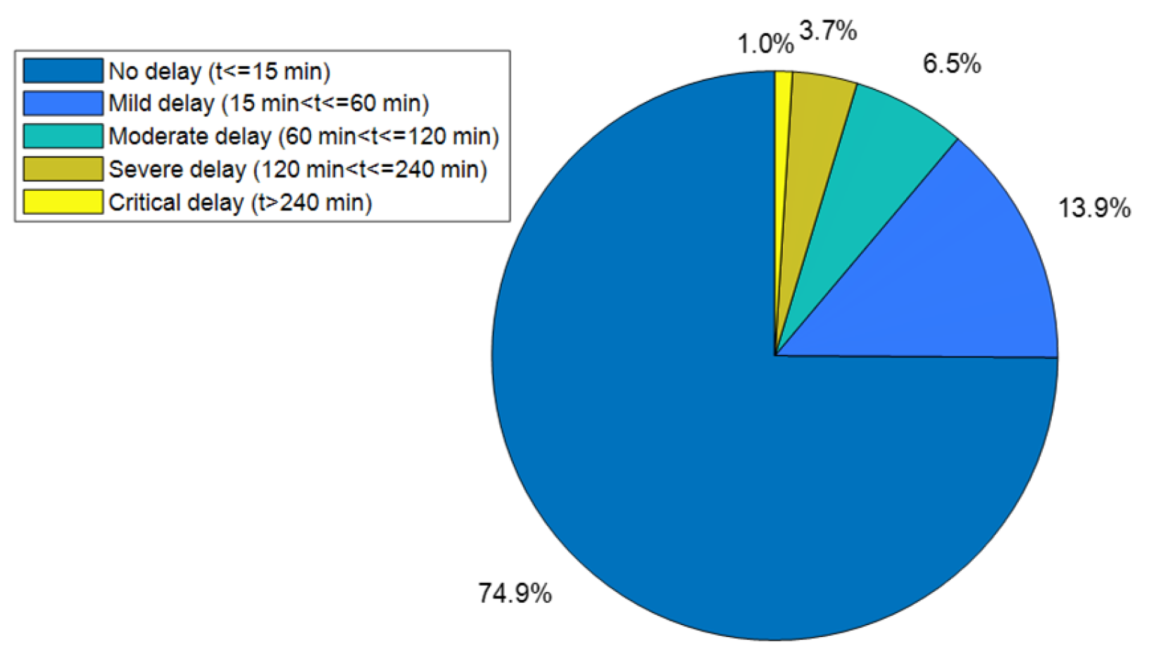
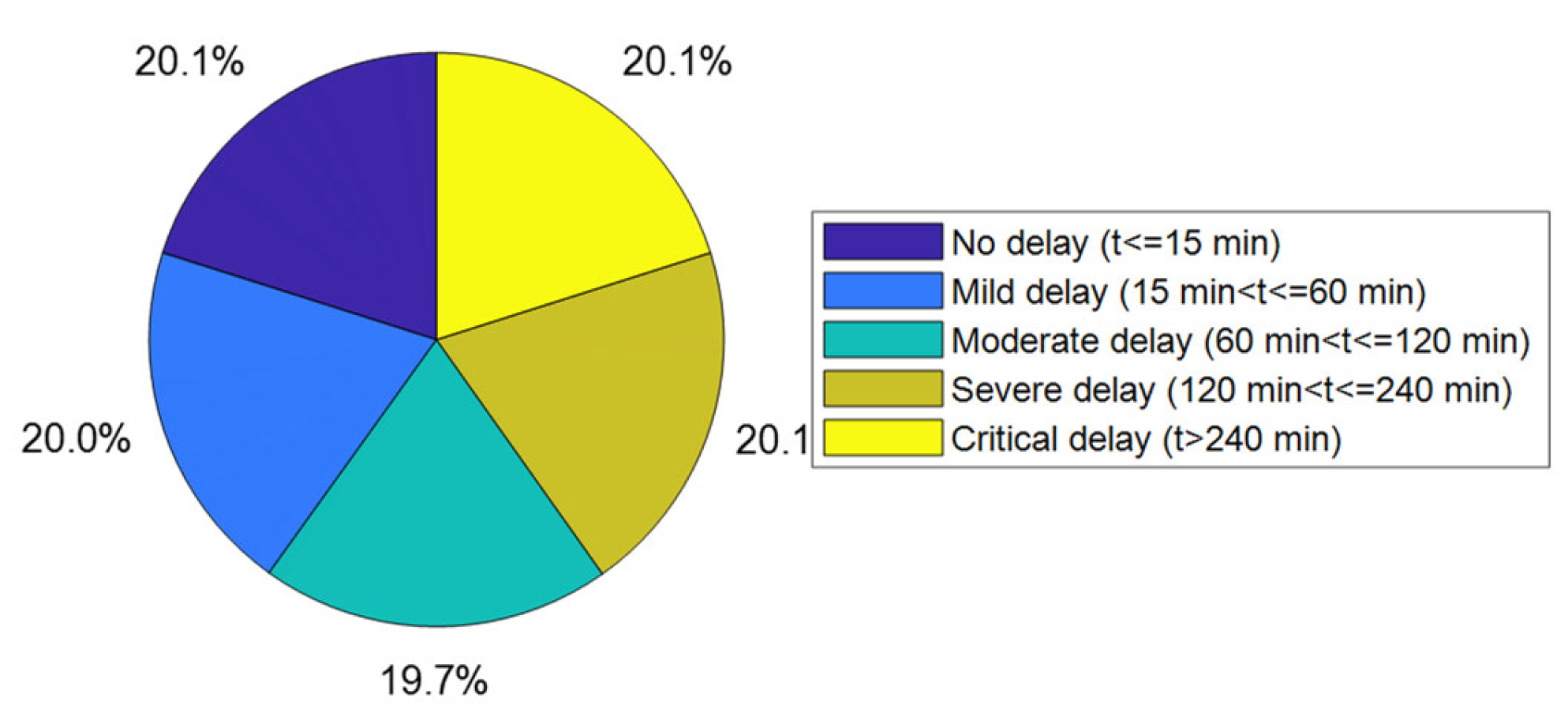
| Level of Delay | Grade Meaning | Slippage Time (At/min) |
|---|---|---|
| 1 | No delayed | At ≤ 15 |
| 2 | Mild Delay | 15 < At ≤ 60 |
| 3 | Moderate Delay | 60 < At ≤ 120 |
| 4 | Severe Delay | 120 < At ≤ 240 |
| 5 | Critical Delay | 240 < At |
| Activation Function | Logsig | Softmax | Tansig | |||
|---|---|---|---|---|---|---|
| Data Set | Training | Testing | Training | Testing | Training | Testing |
| Wbc | 99.71 | 98.62 | 98.67 | 97.52 | 96.57 | 99.29 |
| Balance | 98.31 | 98.02 | 95.41 | 93.51 | 97.82 | 96.83 |
| Iris | 98.62 | 98.14 | 96.36 | 95.13 | 97.26 | 96.42 |
| Glass | 91.26 | 89.32 | 96.81 | 95.41 | 98.41 | 97.67 |
| Pageblocks | 90.23 | 88.42 | 97.52 | 96.38 | 93.45 | 92.26 |
| Segment | 86.51 | 85.13 | 97.42 | 95.61 | 95.62 | 94.29 |
| Texture | 83.47 | 82.87 | 94.79 | 93.26 | 87.27 | 86.41 |
| Pendigits | 81.26 | 80.10 | 93.51 | 92.64 | 90.17 | 89.26 |
| Parameter Settings | FBLS | ||
|---|---|---|---|
| Parameters | r | s | e |
| 110 | 110 | 40 | |
| Modek | Training Set/% | Test Set/% | Accuracy/% | Recall Rate/% | F1 | Time/s |
|---|---|---|---|---|---|---|
| ELM | 17.5469 | 16.5545 | 16.4435 | 16.5425 | 0.1645 | 10.6226 |
| Bayes | 40.0934 | 35.6783 | 35.6673 | 35.6648 | 0.3567 | 6.6554 |
| RBF | 100 | 67.9148 | 67.9012 | 67.8495 | 0.6779 | 80.6415 |
| KNN | 88.5271 | 81.9906 | 81.9852 | 81.9915 | 0.8243 | 1004.5215 |
| BP | 88.0743 | 88.0334 | 88.0235 | 88.0256 | 0.8802 | 65.2154 |
| SVM | 90.2562 | 88.2513 | 88.2655 | 88.3457 | 0.8837 | 85.2155 |
| LSTM | 89.5419 | 88.5446 | 88.4562 | 88.4454 | 0.8850 | 70.2524 |
| CNN | 92.5348 | 90.5348 | 90.5298 | 90.5302 | 0.9053 | 1260.5138 |
| RF | 100 | 92.6337 | 92.5821 | 92.5962 | 0.9260 | 61.2544 |
| LightGBM | 91.5462 | 90.3325 | 90.3015 | 90.3154 | 0.9024 | 136.4562 |
| Xgboost | 84.8545 | 82.6514 | 82.6545 | 82.6351 | 0.822 9 | 391.5559 |
| GBDT | 76.4321 | 72.7536 | 71.4545 | 72.4524 | 0.7213 | 879.3654 |
| Bls | 80.2762 | 79.4621 | 79.2346 | 79.3166 | 0.7834 | 0.0234 |
| Fbls | 97.6652 | 89.8242 | 89.7643 | 89.1346 | 0.89134 | 50.1345 |
| Bp + Bls | 94.5415 | 91.5626 | 91.5654 | 91.5662 | 0.9155 | 70.4563 |
| Rf + bls | 91.5469 | 90.3248 | 90.2365 | 90.2436 | 0.9024 | 72.2563 |
| Cnn + Bls | 96.5424 | 92.3658 | 92.3668 | 92.3754 | 0.9238 | 1500.1349 |
| Cnn + fbls | 98.3164 | 91.6542 | 91.6525 | 91.6564 | 0.9165 | 1608.4304 |
| Bp + fbls | 95.4454 | 91.3556 | 91.3541 | 91.3561 | 0.9136 | 72.5546 |
| DenseNet-LSTM-FBLS | 93.7651 | 92.7141 | 92.7145 | 0.9271 | 86.1246 | 86.1246 |
| Model | Accuracy/% | Precision/% | Recall/% | F1-Score |
|---|---|---|---|---|
| LSTM-FBLS (No Spatial) | 89.15 | 89.08 | 89.05 | 0.8906 |
| CNN-LSTM-FBLS | 91.24 | 91.22 | 91.23 | 0.9122 |
| DenseNet-LSTM-BLS (No Fuzzy) | 91.88 | 91.85 | 91.86 | 0.9185 |
| DenseNet-LSTM-FBLS (Full Model) | 92.71 | 92.71 | 92.71 | 0.9271 |
Disclaimer/Publisher’s Note: The statements, opinions and data contained in all publications are solely those of the individual author(s) and contributor(s) and not of MDPI and/or the editor(s). MDPI and/or the editor(s) disclaim responsibility for any injury to people or property resulting from any ideas, methods, instructions or products referred to in the content. |
© 2025 by the authors. Licensee MDPI, Basel, Switzerland. This article is an open access article distributed under the terms and conditions of the Creative Commons Attribution (CC BY) license (https://creativecommons.org/licenses/by/4.0/).
Share and Cite
Yin, C.; Du, X.; Duan, J.; Tang, Q.; Shen, L. Unveiling Hidden Dynamics in Air Traffic Networks: An Additional-Symmetry-Inspired Framework for Flight Delay Prediction. Mathematics 2025, 13, 2274. https://doi.org/10.3390/math13142274
Yin C, Du X, Duan J, Tang Q, Shen L. Unveiling Hidden Dynamics in Air Traffic Networks: An Additional-Symmetry-Inspired Framework for Flight Delay Prediction. Mathematics. 2025; 13(14):2274. https://doi.org/10.3390/math13142274
Chicago/Turabian StyleYin, Chao, Xinke Du, Jianyu Duan, Qiang Tang, and Li Shen. 2025. "Unveiling Hidden Dynamics in Air Traffic Networks: An Additional-Symmetry-Inspired Framework for Flight Delay Prediction" Mathematics 13, no. 14: 2274. https://doi.org/10.3390/math13142274
APA StyleYin, C., Du, X., Duan, J., Tang, Q., & Shen, L. (2025). Unveiling Hidden Dynamics in Air Traffic Networks: An Additional-Symmetry-Inspired Framework for Flight Delay Prediction. Mathematics, 13(14), 2274. https://doi.org/10.3390/math13142274