Abstract
A well-known model of infectious diseases, described by a nonlinear system of delay differential equations, is investigated under the influence of stochastic perturbations. Using the general method of Lyapunov functional construction combined with the linear matrix inequality (LMI) approach, we derive sufficient conditions for the stability of the equilibria of the considered system. Numerical simulations illustrating the system’s behavior under stochastic perturbations are provided to support the thoretical findings. The proposed method for stability analysis is broadly applicable to other systems of nonlinear stochastic differential equations across various fields.
Keywords:
white noise; Ito’s stochastic differential equation; the general method of constructing Lyapunov functionals; stability in probability; linear matrix inequalities (LMIs) MSC:
60G52; 60H10; 60J65
1. Introduction
The study of mathematical model of infectious diseases has a long history (see, for instance, [1,2,3,4,5,6,7,8,9,10,11,12,13,14,15,16,17,18,19,20,21,22,23,24,25,26,27,28,29,30,31,32,33,34,35,36,37,38,39,40,41,42,43,44,45]) and remains highly relevant today, as it enables the derivation of results that closely reflect real-world processes.
In this article, we examine the spread of an infectious disease from a clinical rather than an epidemiological sense. To provide a mathematical explanation of the disease’s dynamics, it is necessary to first understand its behavior in a therapeutic context. Based on the two primary approaches to the human immune response (humoral and cellular), two corresponding types of mathematical models are developed to describe these mechanisms.
The mechanism of infectious diseases is based on the interaction between antigens (virus) and antibodies, which are represented in the model by the functions and , respectively. Antibodies are understood as components of the immune system (such as immunoglobulins and cell receptors) that neutralize antigens. The population of cells respinsible for carrying and producing antibodies (i.e., immunocompetent cells and immunoglobulin-producing cells) is denoted by . The function represents the extent of organ damage caused by the infection.
First, an antibody binds to an antigen, forming antibody–antigen complexes. In proportion to the quantity of these complexes, plasma cells are produced in the organism after a delay of leading to the mass production of antibodies. The process is described in the first term of the second equation in the system.
If we aim to predict the individual course and outcome of the disease, the basic mathematical model proves inadequate. This is because the model contains unknown parameters, which require a greater number of conditions to generate a reliable solution. Even with daily measurements, which is often impractical, it would still take days to collect sufficient data. By that time, the progression and outcome of the disease would likely be evident without the need for a mathematical model. To address this challenge, the model is individualized through the use of Wiener process-based uncertainty.
The proposed mathematical model of infectious diseases is described by the following system of delay differential equations [39,44]
where are positive parameters; is a body health function defined bellow; represents the immune reaction delay time; and the initial conditions are given by
The first equation of system (1) describes the dynamics of the virus with the following parameters:
- -
- —coefficient describing the antigen activity;
- -
- —the antigen neutralizing factor.
The term describing the rate of change in the plasma cell concentration is represented in the second equation of system (1), where:
- -
- —takes into account the destruction of a normal functioning immune system, m is a feature of the organ;
- -
- —coefficient taking into account the probability of an antigen–antibody meeting;
- -
- —coefficient of reduction of plasma cells due to aging;
- -
- —the plasma cell rate concentration of healthy body.
The dynamics of the antibodies are described by the third equation of the system (1), where:
- -
- —production rate of antibodies by one plasma cell;
- -
- —number of antibodies to neutralize one antigen;
- -
- —the antigen neutralizing factor;
- -
- —coefficient inversely proportional to the decay time of the antibodies.
Finally, the target organ damage rate block is described by the final equation of the system (1), with the following parameters:
- -
- —constant related to a particular disease;
- -
- —coefficient describing the generation rate of the target organ.
Using to the function
where is the threshold value for the relative damage to an organ, we describe the system (1) in two cases
and
Following the work of [44], we transform the system (1) to a dimensionless form. We insert
where are antibodies of a healthy organism and is the maximum antigen’s value, which denotes the following
and we obtain a dimensionless system of the following form:
Remark 1.
The basic system (6) has different types of qualitative solutions. Based on laboratory data on pneumonia, Marchuk G.I. presented different forms of the disease in in [45] by varying the values of the parameters in system (6), which serve as key indicators characterizing the disease:
- -
- for the subclinical form of the disease:
- -
- for the acute form of the disease:
- -
- for the chronic form of the disease:
- -
- for the fatal outcome form of the disease:
2. Equilibria
The equilibria of the system (6) are described using the following system of algebraic equations
2.1. Equilibria and
It is easy to see that regardless of the values of , one of the solutions for the system (11) is the equilibrium . Equilibrium describes the healthy state of an organism.
Using conditions
we can obtain the second equilibrium . From the first Equation (11), it follows that . From the second and third Equation (11), we have . As a result, we obtain:
From the second and final Equation (11), we obtain
Remark 2.
Remark 3.
Note that via (3) for , the obtained must satisfy the condition .
2.2. Equilibria and
Using and , from the second, third, and final Equation (11), we obtain
or
where
or
where
As a result, we obtain two equilibria, and with
and
Remark 5.
- (1)
- For existence and positivity of and , it is required that , , i.e., .
- (2)
- If , then , or equivalently, .
- (3)
- For , it must hold that or , or equivalently .
- (4)
- If is defined, then .
Lemma 1.
For it must hold that:
Proof.
Using (16) and (17), the existence and positivity of require that and . According to (16), for , it must hold that ; and for , the second inequality in (19) must be satisfied. From (17) and (16), we have also have . From , it follows that or
or
from which the last inequality (19) follows. The proof is completed. □
3. Stochastic Perturbations, Centralization, and Linearization
Let be a complete probability space; be a nondecreasing family of sub--algebras of , i.e., for ; let be the probability of an event enclosed in the braces; let be the mathematical expectation with respect to the probability ; and let be the space of -adapted stochastic processes , , , .
Let us suppose that the system (6) in the case of experiences white noise stochastic perturbations, which are directly proportional to the deviation of the system state from one of the equilibria . So, we obtain the system of Ito’s stochastic differential equations [31,46]
where are constants and are mutually independent -measurable Wiener processes on the probability space .
Remark 6.
It is clear that the equilibrium of the system for deterministic differential Equation (6) is also the solution for the system of stochastic differential Equation (20). Note that the first stochastic perturbations for (20) were used in [13] and later in man other works (see, for instance, [31] and the references therein).
By adding new variables into (20)
and using (11), we obtain a nonlinear system of stochastic delay differential equations with the zero solution
Matrix Form
Note that the linear part (22) of the systems (21) can be represented in the matrix form
where (here and everywhere below, ′ indicates transposition),
the matrix
In particular, for equilibrium , matrices A and B are
and, similarly, for equilibrium
where and are defined in (13).
4. Stability
Definition 1.
Definition 2.
The zero solution of the system (22) with the initial condition , , is called:
- -
- mean square stable if for each there exists a such that , , provided that ;
- -
- asymptotically mean square stable if it is mean square stable and for each initial function ϕ.
Remark 7.
The stability of the zero solution of system (21) is equivalent to the stability of the equilibrium point of system (20). It is important to note that the system of nonlinear stochastic differential Equation (21) shows a degree of nonlinearity greater than one. As shown in [31], in such cases, sufficient conditions for the asymptotic mean square stability of the zero solution of the linearized system (22) are also sufficient for the stability in probability of the zero solution of the full nonlinear system (21).
Below, and denote the value of the solution at time t and a complete trajectory of the solution up to time t, respectively.
Consider a functional that can be represented in the form , , and for put
Let D be the set of functionals, for which the function defined by (27) has a continuous derivative with respect to t and two continuous derivatives with respect to y. The generator L of Equation (23) is defined by the functionals from D and has the following form [31,46]
Theorem 1
([31]). Let a functional and positive constants , , exist, such that the following conditions hold:
Then, the zero solution of the system (22) is asymptotically mean square stable.
Theorem 2.
Proof.
Using Remark 7, to prove the stability in probability of the equilibrium of system (20), it is enough to prove the asymptotic mean square stability of the zero solution of Equation (23). Using the general method of Lyapunov functional construction [31], let us construct the functional , where and are chosen below. Let L be the generator [31,46] of Equation (23). Then
Using the additional functional , we have
As a result, from (30), (31) for the functional , and some , we obtain
Using Theorem 1, we know that the zero solution of Equation (23) is asymptotically mean square stable. The proof is completed. □
4.1. Routh–Hurwitz Criterion
Definition 3
([31]). The trace of the k-th order of an -matrix A with elements is defined as follows
Here, in particular, , .
The characteristic equation of the matrix in Equation (23) has the following form
It is known [31] that for LMI (29), all roots of the characteristic Equation (33) must have negative real parts.
Theorem 3
([31]). (Routh–Hurwitz criterion) All roots λ of the characteristic Equation (33) have negative real parts, if and only if
4.2. Equilibrium
Theorem 4.
If
then, the equilibrium is stable in probability.
Proof.
It is clear that the stability of equilibrium is equivalent to the stability of the zero solution of the system (21). The order of nonlinearity of the nonlinear system (21) is higher than one. Following Remark 7 for stability in probability of the equilibrium , it is enough to prove the asymptotic mean square stability of the zero solution of the linear system (22).
It is known [31] that the first inequality (36) is a necessary and sufficient condition for the asymptotic mean square stability of the zero solution of the first Equation (22). Using and the second and final inequalities (36), we obtain that and converge to zero too. Similarly, from , and the third inequality (36), it follows that . The proof is completed. □
4.3. Equilibria and
5. Numerical Simulations
Let us consider some examples for the equilibria , , , discussed in Figure 1, Figure 2 and Figure 3.
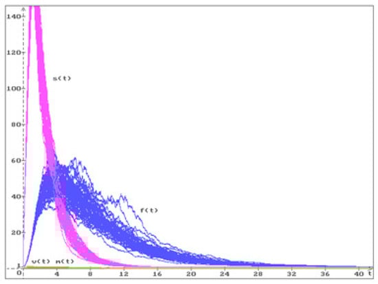
Figure 1.
50 trajectories of the solution (), of the system (20) converge to the stable equilibrium .
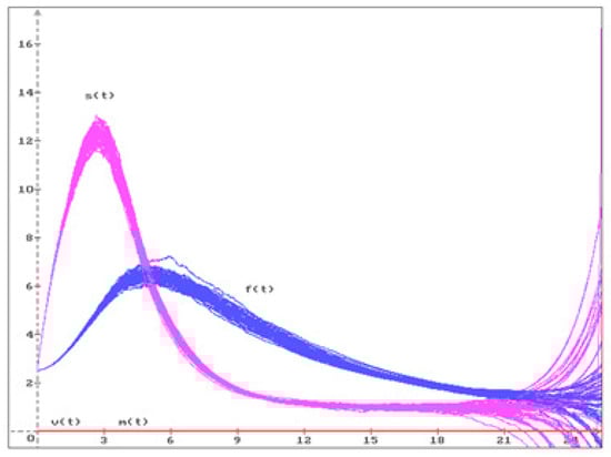
Figure 2.
50 trajectories of the solution (), of the system (20) move away from the unstable equilibrium .
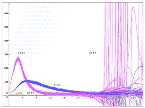
Figure 3.
50 trajectories of the solution (), of the system (20) move away from the unstable equilibrium .
Example 2.
Consider the system (20) with the parameters (7) and
Using MATLAB (R2024a), it was shown that for equilibrium with the parameters from (7) and (38), LMI (29) holds, i.e., this equilibrium is stable in probability. In Figure 1, 50 trajectories from the system (20) solution are shown with the following initial conditions
The state of a healthy organism in the case (7) corresponds to the equilibrium
Example 3.
Consider equilibrium with the parameters from (8). In accordance with (14) and Remark 3, we obtain the following values for the equilibrium = . According to Remark 9, this equilibrium is unstable, even in the deterministic case. In Figure 2 50 trajectories of the system (20) solution are shown with , and the initial conditions
which are close enough to equilibrium . It can be seen that all trajectories move away from the unstable equilibrium.
Example 4.
Consider equilibrium with the parameters of (10). Using (17) and (18), we obtain
According to Remark 9, this equilibrium is unstable. In Figure 3, 50 trajectories of the system (20) solution are shown with , and the following initial conditions
which are close enough to equilibrium . All trajectories move away from the unstable equilibrium.
Remark 10.
Figure 1, Figure 2 and Figure 3 show that equilibrium is stable, and equilibria and are unstable. According to our results, from a medical point of view, it is shown that only a healthy body is in a stable state, while in other cases of equilibria, there is a high probability that the patient’s condition will change soon.
6. Conclusions
The known deterministic model of infectious diseases, proposed by G.I. Marchuk, is studied under stochastic perturbations and is described by a system of Ito’s stochastic differential equations with a delay. Conditions of stability or instability of equilibria for the considered system are investigated. We provide examples of numerical simulations for the system solutions and figures that illustrate the obtained results. The proposed research method can be used to investigate other nonlinear mathematical models in various applications.
Author Contributions
Methodology, M.B. and L.S. All authors have read and agreed to the published version of the manuscript.
Funding
This research received no external funding.
Data Availability Statement
The authors did not use any special data supporting the obtained results in this paper, besides the literature included in the references.
Conflicts of Interest
The authors declare no conflicts of interest.
References
- Bailey, N.T.J. The Mathematical Theory of Infectious Diseases and Its Applications, 2nd ed.; Charles Griffin & Company Ltd.: London, UK, 1975. [Google Scholar]
- Bartlett, M.S. Deterministic and stochastic models for recurrent epidemics. In Proceedings of the 3rd Berkeley Symposium on Mathematical Statistics and Probability, Berkeley, CA, USA, 26–31 December 1956; Volume 4, pp. 81–109. [Google Scholar]
- Hege, J.S.; Cole, G. A mathematical model relating circulating antibody and antibody forming cells. J. Immunol. 1966, 97, 34–40. [Google Scholar] [CrossRef] [PubMed]
- Kermack, W.O.; McKendrick, A.G. A contribution to the mathematical theory of epidemics. Proc. R. Soc. Lond. Ser. A 1927, 115, 700–721. Available online: https://royalsocietypublishing.org/doi/10.1098/rspa.1927.0118 (accessed on 20 June 2025).
- Ross, R. The Prevention of Malaria; E.P. Dutton and Company: New York, NY, USA, 1910; Available online: https://archive.org/details/pr00eventionofmalarossrich/mode/2up (accessed on 20 June 2025).
- Bernoulli, D.; Blower, S. An attempt at a new analysis of the mortality caused by smallpox and of the advantages of inoculation to prevent it. Rev. Med. Virol. 2004, 14, 275–288. [Google Scholar] [CrossRef] [PubMed]
- Farr, W. Report on the Mortality of Cholera in England, 1848–1849, Great Britain; General Register Office; Royal College of Physicians of London (HMSO): London, UK, 1852; Available online: https://wellcomecollection.org/works/pajtrpez (accessed on 20 June 2025).
- Bruni, C.; Giovenco, M.A.; Koch, G.; Strom, R. A dynamical model of humoral immune response. Math. Biosci. 1975, 27, 191–211. [Google Scholar] [CrossRef]
- Bell, G.I. Mathematical model of clonal selection and antibody production. J. Theor. Biol. 1970, 29, 191–232. [Google Scholar] [CrossRef]
- Albani, V.V.L.; Zubelli, J.P. Stochastic transmission in epidemiological models. J. Math. Biol. 2024, 88, 25. [Google Scholar] [CrossRef]
- Allen, L.J.S. A primer on stochastic epidemic models: Formulation, numerical simulation, and analysis. Infect. Dis. Model. 2017, 2, 128–142. [Google Scholar] [CrossRef]
- Andersson, H.; Britton, T. Stochastic Epidemic Models and Their Statistical Analysis; Volume 151 of Lecture Notes in Statistics; Springer: New York, NY, USA, 2000. [Google Scholar] [CrossRef]
- Beretta, E.; Kolmanovskii, V.; Shaikhet, L. Stability of epidemic model with time delays influenced by stochastic perturbations. Math. Comput. Simul. 1998, 45, 269–277. [Google Scholar] [CrossRef]
- Beretta, E.; Takeuchi, Y. Global stability of an SIR epidemic model with time delays. J. Math. Biol. 1995, 33, 250–260. [Google Scholar] [CrossRef]
- Bouzalmat, I.; El Idrissi, M.; Settati, A.; Lahrouz, A. Stochastic SIRS epidemic model with perturbation on immunity decay rate. J. Appl. Math. Comput. 2023, 69, 4499–4524. [Google Scholar] [CrossRef]
- Britton, T. Stochastic epidemic models: A survey. Math. Biosci. 2010, 225, 24–35. [Google Scholar] [CrossRef] [PubMed]
- Cai, Y.; Kang, Y.; Banerjee, M.; Wang, W. A stochastic SIRS epidemic model with infectious force under intervention strategies. J. Differ. Equ. 2015, 259, 7463–7502. [Google Scholar] [CrossRef]
- Cai, Y.; Kang, Y.; Wang, W. A stochastic SIRS epidemic model with nonlinear incidence rate. Appl. Math. Comput. 2017, 305, 221–240. [Google Scholar] [CrossRef]
- Dieu, N.T.; Nguyen, D.H.; Du, N.H.; Yin, G. Classification of asymptotic behaviour in a stochastic SIR model. SIAM J. Appl. Dyn. Syst. 2016, 15, 1062–1084. [Google Scholar] [CrossRef]
- Gray, A.J.; Greenhalgh, D.; Hu, L.; Mao, X.; Pan, J. A stochastic differential equation SIS epidemic model. SIAM J. Appl. Dyn. Syst. 2011, 71, 876–902. [Google Scholar] [CrossRef]
- Greenwood, P.E.; Gordillo, L.F. Stochastic epidemic modeling. In Mathematical and Statistical Estimation Approaches in Epidemiology; Springer: Dordrecht, The Netherlands, 2009; pp. 31–52. [Google Scholar] [CrossRef]
- Karako, K.; Song, P.; Chen, Y.; Tang, W. Analysis of COVID-19 infection spread in japan based on stochastic transition model. Biosci. Trends 2020, 14, 134–138. [Google Scholar] [CrossRef]
- Kiss, I.Z.; Miller, J.C.; Simon, P.L. Mathematics of Epidemics on Networks, From Exact to Approximate Models; Springer: Berlin, Germany, 2017. [Google Scholar]
- Korobeinikov, A. Global properties of SIR and SEIR epidemic models with multiple parallel infectious stages. Bull. Math. Biol. 2009, 71, 75–83. [Google Scholar] [CrossRef]
- Laaribi, A.; Boukanjime, B.; El Khalifi, M.; Bouggar, D.; El Fatini, M. A generalized stochastic SIRS epidemic model incorporating mean-reverting ornstein–uhlenbeck process. Phys. A Stat. Mech. Appl. 2023, 615, 128609. [Google Scholar] [CrossRef]
- Lahrouz, A.; Settati, A.; El Fatini, M.; Tridane, A. The effect of a generalized nonlinear incidence rate on the stochastic SIS epidemic model. Math. Methods Appl. Sci. 2021, 44, 1137–1146. [Google Scholar] [CrossRef]
- Martcheva, M. An Introduction to Mathematical Epidemiology; Texts in Applied Mathematics; Springer: New York, NY, USA, 2010; Volume 61. [Google Scholar] [CrossRef]
- Nguyen, T.D.; Takasu, F.; Nguyen, H.D. Asymptotic behaviours of stochastic epidemic models with jump-diffusion. Appl. Math. Model. 2020, 86, 259–270. [Google Scholar] [CrossRef]
- Settati, A.; Caraballo, T.; Lahrouz, A.; Bouzalmat, T.; Assadouq, A. Stochastic SIR epidemic model dynamics on scale-free networks. Math. Comput. Simul. 2025, 229, 246–259. [Google Scholar] [CrossRef]
- Settati, A.; Lahrouz, A.; Zahri, M.; Tridane, A.; El Fatini, M.; El Mahjour, H.; Seaid, M. A stochastic threshold to predict extinction and persistence of an epidemic SIRS system with a general incidence rate. Chaos Solit. Fractals 2021, 144, 110690. [Google Scholar] [CrossRef]
- Shaikhet, L. Lyapunov Functionals and Stability of Stochastic Functional Differential Equations; Springer Science & Business Media: Berlin/Heidelberg, Germany, 2013. [Google Scholar] [CrossRef]
- Tesfay, A.; Saeed, T.; Zeb, A.; Tesfay, D.; Khalaf, A.; Brannan, J. Dynamics of a stochastic COVID-19 epidemic model with jump-diffusion. Adv. Differ. Equ. 2021, 2021, 228. [Google Scholar] [CrossRef]
- Tornatore, E.; Vetro, P.; Buccellato, S.M. SIVR epidemic model with stochastic perturbation. Neural Comput. Appl. 2014, 24, 309–315. [Google Scholar] [CrossRef]
- Zhang, X.; Wang, K. Stochastic SIR model with jumps. Appl. Math. Lett. 2013, 26, 867–874. [Google Scholar] [CrossRef]
- Zhang, Z.; Zeb, A.; Hussain, S.; Alzahrani, E. Dynamics of COVID-19 mathematical model with stochastic perturbation. Adv. Differ. Equ. 2020, 2020, 451. [Google Scholar] [CrossRef]
- Zhao, D.; Yuan, S. Threshold dynamics of the stochastic epidemic model with jump-diffusion infection force. J. Appl. Anal. Comput. 2019, 9, 440–451. [Google Scholar] [CrossRef]
- Zhou, Y.; Zhang, W. Threshold of a stochastic SIR epidemic model with Levy jumps. Phys. A Stat. Mech. Appl. 2016, 446, 204–216. [Google Scholar] [CrossRef]
- Zhou, Y.; Zhang, W.; Yuan, S. Survival and stationary distribution of a SIR epidemic model with stochastic perturbations. Appl. Math. Comput. 2014, 244, 118–131. [Google Scholar] [CrossRef]
- Marchuk, G.I. Mathematical Modelling of Immune Response in Infection Diseases; Book series: Mathematics and Its Applications; Springer Science & Business Media: Dordrecht, The Netherlands, 1997. [Google Scholar] [CrossRef]
- Domoshnitsky, A.; Bershadsky, M.; Volinsky, I. Distributed control in stabilization of a model of infection diseases. Russ. J. Biomech. 2019, 23, 494–499. [Google Scholar] [CrossRef]
- Domoshnitsky, A.; Volinsky, I.; Bershadsky, M. Around the Model of Infection Disease: The Cauchy Matrix and Its Properties. Symmetry 2019, 11, 1016. [Google Scholar] [CrossRef]
- Volinsky, I.; Bershadsky, M. Numerical Solution of Marchuk models of infection diseases. Funct. Differ. Equ. 2021, 28, 85–93. Available online: https://www.ariel.ac.il/wp/fde/2021/03/21/numerical-solution-of-marchuk-model-of-infection-diseases/ (accessed on 20 June 2025). [CrossRef]
- Volinsky, I.; Domoshnitsky, A.; Bershadsky, M.; Shklyar, R. Marchuk’s Models of Infection Diseases: New Developments. In Functional Differential Equations and Applications; FDEA, 2019; Domoshnitsky, A., Rasin, A., Padhi, S., Eds.; Springer Proceedings in Mathematics and Statistics; Springer: Singapore, 2021; Volume 379, pp. 131–143. [Google Scholar] [CrossRef]
- Bershadsky, M.; Chirkov, M.; Domoshnitsky, A.; Rusakov, S.; Volinsky, I. Distributed Control and the Lyapunov Characteristic Exponents in the Model of Infectious Diseases. Complexity 2019, 5234854. [Google Scholar] [CrossRef]
- Marchuk, G.I. Mathematical Models in Immunology; Nauka: Moscow, Russia, 1980. [Google Scholar]
- Gikhman, I.I.; Skorokhod, A.V. Stochastic Differential Equations; Springer: Berlin/Heidelberg, Germany, 1972. [Google Scholar]
Disclaimer/Publisher’s Note: The statements, opinions and data contained in all publications are solely those of the individual author(s) and contributor(s) and not of MDPI and/or the editor(s). MDPI and/or the editor(s) disclaim responsibility for any injury to people or property resulting from any ideas, methods, instructions or products referred to in the content. |
© 2025 by the authors. Licensee MDPI, Basel, Switzerland. This article is an open access article distributed under the terms and conditions of the Creative Commons Attribution (CC BY) license (https://creativecommons.org/licenses/by/4.0/).