Image Inpainting with Fractional Laplacian Regularization: An L^p Norm Approach

Abstract

This study presents an image inpainting model based on an energy functional that incorporates the $L^p$ norm of the fractional Laplacian operator as a regularization term and the $H^{-1}$ norm as a fidelity term. Using the properties of the fractional Laplacian operator, the $L^p$ norm is employed with an adjustable parameter p to enhance the operator’s ability to restore fine details in various types of images. The replacement of the conventional $L^2$ norm with the $H^{-1}$ norm enables better preservation of global structures in denoising and restoration tasks. This paper introduces a diffusion partial differential equation by adding an intermediate term and provides a theoretical proof of the existence and uniqueness of its solution in Sobolev spaces. Furthermore, it demonstrates that the solution converges to the minimizer of the energy functional as time approaches infinity. Numerical experiments that compare the proposed method with traditional and deep learning models validate its effectiveness in image inpainting tasks.

1. Introduction

Image inpainting is a vital task in image processing, with applications ranging from restoring old paintings and removing unwanted scratches or text from images to recovering lost data during transmission. Mathematically, images are considered as functions defined on a continuum, though in practice, digital images are discrete representations of their continuous counterparts. Formally, a digital image can be represented as a matrix $u\in {\mathbb{R}}^{I\times J}$. Due to various interferences in the image acquisition and transmission processes, the observed image data, $u_0\in {\mathbb{R}}^{I\times J}$, is often expressed as

$$u_0=\mathcal{A}u+\eta ,$$

(1)

where $\mathcal{A}$ is a degenerate operator and $\eta \in {\mathbb{R}}^{I\times J}$ is a random noise, typically assumed to be white Gaussian noise in this context.  Thus, image inpainting becomes an inverse problem where the goal is to estimate $u^{\ast }\in {\mathbb{R}}^{I\times J}$ from $u_0$. The problem is ill-posed, making its solution nontrivial and requiring specialized methods for effective restoration.

A variety of techniques have been proposed to solve the image inpainting problem. Among the most widely used are diffusion-based methods, which leverage the information from neighboring regions to propagate data into damaged areas. These methods typically use partial differential equation (PDE)-based and variational-based frameworks for image restoration. Bertalmio et al. [1] introduced the first PDE-based inpainting model, which was simple but prone to producing blurred results due to the smoothness of differential operators. Subsequent work [2,3] sought to refine this approach by improving the handling of image features, but the issue of blur remained.

Variational methods, based on minimizing an appropriately designed energy functional, have become another cornerstone of image inpainting. A typical variational formulation is given by

$$\underset{u\in {\mathbb{R}}^{I\times J}}{min}\left\{{\displaystyle \frac{1}{2}}\left|\right|\mathcal{A}u-u_0{\left|\right|}_F^2+\lambda \mathcal{R}\left(u\right)\right\},$$

(2)

where $\lambda >0$ is a regularization parameter, and $\mathcal{R}\left(u\right)$ is a regularization term that controls the smoothness of the solution.  Total variation (TV) models, introduced by Chan and Shen [4], are particularly popular due to their ability to preserve edges while filling in missing regions. However, TV methods often struggle with large missing areas or disconnected regions, leading to the staircase effect [5].  To address these issues, higher-order models such as those by Lysaker et al. [6] and adaptive PDE methods have been developed, offering improved smoothness and edge preservation [7,8].

In recent years, fractional-order PDEs have gained attention for image processing, offering better control over the smoothness and sharpness of restored images.  Fractional differential operators replace standard differential operators with their fractional counterparts, leading to models that mitigate the oversmoothing effect commonly observed in traditional PDE-based methods [9,10]. These fractional models have shown promising results in both theoretical studies and practical applications [11,12,13,14,15,16,17,18,19,20,21,22,23,24,25,26,27,28].

Another notable approach to image inpainting is exemplar-based methods, which grow image regions pixel by pixel or patch by patch while maintaining coherence with the surrounding texture. These methods, popularized by Criminisi et al. [29], are especially effective in images with repetitive textures but struggle in the absence of suitable matching samples. Recent work has improved these methods by introducing nonlocal techniques [30,31] and hierarchical schemes [32], though structural connectivity remains a challenge.

In more recent years, deep learning-based inpainting techniques have achieved impressive results by leveraging generative models, such as Variational Autoencoders (VAEs) [33,34] and Generative Adversarial Networks (GANs) [35,36], to learn both high- and low-frequency features of the image. These models generate plausible content for missing regions by learning the underlying structure and texture of the image. Several architectures have been proposed to address different types of inpainting challenges, such as irregular hole filling [37], high-resolution restoration [38], and multiple-solution generation [39].

In the context of image inpainting, the use of the fractional Laplacian has gained significant interest in recent years. The fractional Laplacian, a nonlocal operator, provides a more accurate representation of spatial interactions compared to traditional local differential operators. The operator is defined as

$${(-\Delta )}^{{\displaystyle \frac{\alpha }{2}}}u\left(x\right):=C_{n,\alpha }P.V.{\int }_{R^n}{\displaystyle \frac{u\left(x\right)-u\left(y\right)}{{|x-y|}^{n+\alpha }}}\mathrm{d}y,$$

(3)

$$C_{n,\alpha }={\displaystyle \frac{2^{\alpha }\mathsf{\Gamma }\left(\frac{n+\alpha }{2}\right)}{{\pi }^{\frac{n}{2}}\left|\mathsf{\Gamma }(-\frac{\alpha }{2})\right|}}.$$

where $\alpha$ is any real number between 0 and 1, and $P.V.$ denotes the principal value of the integral.  Recent work [40,41] has focused on numerical methods for discretizing the fractional Laplacian, demonstrating its ability to improve image quality while avoiding the oversmoothing problem common to traditional methods.

Our original model [23] was based on the fractional Laplacian operator with the $L^2$ norm serving as the regularization term and the $L^2$ norm as the fidelity term. However, the paper lacked a theoretical proof of the solution to the diffusion equation. This article primarily explores the application of the fractional Laplacian operator in image inpainting tasks, and the inpainting results are quite promising. This paper represents an optimization of the original model which uses the $L^p$ norm of fractional Laplacian operator as the regularization term and the $L^2$ norm as the fidelity term and completes the theoretical framework. The inpainting results not only surpass those of the original model but also outperform some other models that were previously incomparable.

In summary, the main contributions of this work are as follows:

• Proposal of a novel image inpainting model: We introduce an image inpainting model based on an energy functional that combines the $L^p$ norm of the fractional Laplacian operator as a regularization term and the $H^{-1}$ norm as a fidelity term.
• Theoretical derivation of the PDE system: We rigorously derive the Euler–Lagrange equations and the corresponding nonlinear partial differential equation (PDE) system within the variational framework. We prove the existence and uniqueness of weak solutions to this PDE system and show that, as time tends to infinity, the weak solution converges to the minimizer of the original energy functional.
• Stable numerical method: We design a stable numerical method for solving the PDE system, provide a discrete scheme for the fractional Laplacian operator, and conduct a theoretical analysis of the method’s stability and convergence.

2. Proposed Model

First of all, we explain some notation used in this paper. We use notation $\mathcal{F}$ stands for Fourier transform defined as

$$\left(\mathcal{F}u\right) \left(\xi \right)={\int }_{{\mathbb{R}}^n}u\left(x\right)e^{-ix·\xi }\mathrm{d}x,$$

where i stands for the imaginary unit, and $u\in L^1\left({\mathbb{R}}^n\right)$. We use $𝒮\left({\mathbb{R}}^n\right)$ to indicate Schwartz space. For $u\in 𝒮\left({\mathbb{R}}^n\right)$, the fractional Laplacian operator ${(-\Delta )}^{{\displaystyle \frac{\alpha }{2}}}u$ is defined as

$${(-\Delta )}^{{\displaystyle \frac{\alpha }{2}}}u={\mathcal{F}}^{-1}\left({\left|\xi \right|}^{\alpha }\left(\mathcal{F}u\right)\left(\xi \right)\right).$$

The generalized fractional Laplacian operator is defined on distribution space ${𝒮}^{\prime }\left({\mathbb{R}}^n\right)$, which is dual space of $𝒮\left({\mathbb{R}}^n\right)$, as

$$⟨{(-\Delta )}^{\frac{\alpha }{2}}u,\phi ⟩=⟨u,{(-\Delta )}^{\frac{\alpha }{2}}\phi ⟩:={\int }_{{\mathbb{R}}^n}u{(-\Delta )}^{\frac{\alpha }{2}}\phi \mathrm{d}x,\forall \phi \in 𝒮\left({\mathbb{R}}^n\right).$$

Using the above notation, we define the Bessel potential space.

Definition 1 (Bessel potential space).

Let $\alpha >0,1<p<\infty$; the Bessel potential space is defined as

$$H^{\alpha ,p}\left({\mathbb{R}}^n\right)=\left\{u\in L^p\left({\mathbb{R}}^n\right):{\mathcal{F}}^{-1}\left({(1+|\xi |}^2{)}^{\frac{\alpha }{2}}\left(\mathcal{F}u\right)\right)\in L^p\left({\mathbb{R}}^n\right)\right\}.$$

The norm of Bessel potential space is defined as

$${∥u∥}_{H^{\alpha ,p}\left({\mathbb{R}}^n\right)}:={∥{\mathcal{F}}^{-1}\left({(1+|\xi |}^2{)}^{\frac{\alpha }{2}}\left(\mathcal{F}u\right)\right)∥}_{L^p\left({\mathbb{R}}^n\right)}.$$

This space has some special properties that we need to use in the subsequent proof. We can see the proof in proposition 3.10 and proposition 3.15 in [42].

Theorem 1.

For every $\alpha >0,1<p<\infty$, the space $H^{\alpha ,p}\left({\mathbb{R}}^n\right)$ is complete and separable.

Theorem 2 (Fractional Sobolev embedding theorem).

Let $\alpha >0,1<p<\infty$, then

• If $\alpha p<n$, then:

  $$H^{\alpha ,p}\left({\mathbb{R}}^n\right)\hookrightarrow L^q\left({\mathbb{R}}^n\right),q\in [p,{\displaystyle \frac{np}{n-\alpha p}}],$$
  and the embedding is continuous.
• If $\alpha p=n$, then

  $$H^{\alpha ,p}\left({\mathbb{R}}^n\right)\hookrightarrow L^q\left({\mathbb{R}}^n\right),q\in [p,\infty ],$$
  and the embedding is continuous.
• If $\alpha p>n$, then

  $$H^{\alpha ,p}\left({\mathbb{R}}^n\right)\hookrightarrow C^{\lfloor \alpha \rfloor ,\mu }\left({\mathbb{R}}^n\right),0<\mu \le \alpha -{\displaystyle \frac{n}{p}},$$
  and the embedding is continuous.
• Let $0<t<\alpha ,1<p<\infty$, then

  $$H^{\alpha ,p}\left({\mathbb{R}}^n\right)\hookrightarrow H^{t,p}\left({\mathbb{R}}^n\right),$$
  and the embedding is continuous.
• Let $0<t<\alpha ,1<p<\infty$ such that $(\alpha -t)p<n$, then

  $$H^{\alpha ,p}\left({\mathbb{R}}^n\right)\hookrightarrow H^{t,q}\left({\mathbb{R}}^n\right),$$
  with

  $$q:={\displaystyle \frac{np}{n-(\alpha -t)p}},$$
  the embedding is continuous.

When processing an image u defined on a finite domain, we need to extend it to the entire space ${\mathbb{R}}^n$ while preserving required regularity conditions. Let $\mathsf{\Omega }\subset {\mathbb{R}}^n$ be a finite Lipschitz domain. The extension of u to ${\mathbb{R}}^n$, denoted by $\tilde{u}$, must satisfy the following requirements:

$$\begin{array}{cc}\hfill & \tilde{u}{|}_{\mathsf{\Omega }}=u;\hfill \\ \hfill & {∥\tilde{u}∥}_{L^p\left({\mathbb{R}}^n\right)}\le C{∥u∥}_{L^p\left(\mathsf{\Omega }\right)},\exists C>0.\hfill \end{array}$$

(4)

Without the loss of generality, we use u to represent the extension function $\tilde{u}$, and the subsequent function extensions in the paper will be constructed following this approach, such that the fractional Laplacian operator for the function u defined on the region $\mathsf{\Omega }$ can be expressed as

$${(-\Delta )}^{{\displaystyle \frac{\alpha }{2}}}u={(-\Delta )}^{{\displaystyle \frac{\alpha }{2}}}\tilde{u},$$

where $\tilde{u}$ is the extension of u.

We expand the definition of Bessel potential space in domain $\mathsf{\Omega }$.

Definition 2.

The Bessel potential space $H_0^{\alpha ,p}\left(\mathsf{\Omega }\right)$ defined on the open set $\mathsf{\Omega }\subset {\mathbb{R}}^n$ is defined as

$$H_0^{\alpha ,p}\left(\mathsf{\Omega }\right)=\left\{u\in H^{\alpha ,p}\left({\mathbb{R}}^n\right): \mathrm{supp}u\subset \overline{\mathsf{\Omega }}\right\}.$$

The norm is defined as

$${∥u∥}_{H_0^{\alpha ,p}\left(\mathsf{\Omega }\right)}:={∥u∥}_{H^{\alpha ,p}\left({\mathbb{R}}^n\right)}.$$

Theorem 3.

Let $\mathsf{\Omega }\subset {\mathbb{R}}^n$ be a Lipschitz domain, then there exists a bounded linear extension operator:

$$E:H_0^{\alpha ,p}\left(\mathsf{\Omega }\right)\hookrightarrow H^{\alpha ,p}\left({\mathbb{R}}^n\right),$$

such that ${E\left(u\right)|}_{\mathsf{\Omega }}=u$.

By Theorem 3, Theorem 2 is established for Lipschitz domains.

Theorem 4

(Equal norm in $H_0^{\alpha ,p}\left(\mathsf{\Omega }\right)$). The norm

$$∥·∥={∥·∥}_{L^p\left(\mathsf{\Omega }\right)}+{∥{(-\Delta )}^{\frac{\alpha }{2}}(·)∥}_{L^p\left(\mathsf{\Omega }\right)},$$

is equivalent to ${∥·∥}_{H_0^{\alpha ,p}\left(\mathsf{\Omega }\right)}$ in $H_0^{\alpha ,p}\left(\mathsf{\Omega }\right)$.

2.1. Inpainting Model

Suppose that $\mathsf{\Omega }\subset {\mathbb{R}}^n$ is Lipschitz domain and $D\subset \mathsf{\Omega }$ is a closed set representing the inpainting area, $\alpha \in (0,2)$, $p\in (1,2]$, and $\lambda >0$. Let

$$\begin{array}{cc}\hfill J\left(u\right)=& {∥{(-\Delta )}^{\frac{\alpha }{2}}u∥}_{L^p\left(\mathsf{\Omega }\right)}^p+\frac{\lambda }{2}{∥u-u_0∥}_{H^{-1}(\mathsf{\Omega }\setminus D)}^2\hfill \\ \hfill =& {\int }_{\mathsf{\Omega }}{\left|{(-\Delta )}^{\frac{\alpha }{2}}u\right|}^p\mathrm{d}x+{\displaystyle \frac{\lambda }{2}}{\int }_{\mathsf{\Omega }\setminus D}{\left|\nabla {\Delta }^{-1}(u-u_0)\right|}^2\mathrm{d}x,\hfill \end{array}$$

(5)

then our inpainting model is

$$u^{\ast }=\underset{u\in H_0^{\alpha ,p}\left(\mathsf{\Omega }\right)\cap H^{-1}\left(\mathsf{\Omega }\right)}{arg~min}J\left(u\right).$$

(6)

Our model consists of two terms. The first one is the p-power of $L^p$ norm of ${(-\Delta )}^{\frac{\alpha }{2}}u$, and the second term represents the square of $H^{-1}$ norm for $u-u_0$, where the distribution space $H^{-1}$ is the dual space of $H_0^1$. The first time using $H^{-1}$ norm in image inpainting is in [43], in which it is said that not only $L^2\left(\mathsf{\Omega }\right)\subset H^{-1}\left(\mathsf{\Omega }\right)$ but also this norm can better separate oscillatory components from high-frequency components compared to the $L^2$ norm, while also being better at removing noise while preserving edges.

Remark 1.

The operator ${\Delta }^{-1}$ represents the weak inverse of Δ. Given an open set $E,{\Delta }^{-1}:L^2\left(E\right)\to H_0^1\left(E\right)$ is defined as follows: $\forall f\in L^2\left(E\right)$ ${\Delta }^{-1}f$ is the unique week solution of PDE (7) in space $H_0^1\left(E\right)$:

$$\left\{\begin{array}{cc}\Delta \phi =f,\hfill & \hfill x\in E,\\ \phi =0,\hfill & \hfill x\in \mathsf{\partial }E.\end{array}\right.$$

(7)

In other words, ${\Delta }^{-1}f=\phi$, where φ is a weak solution of Equation (7) that satisfies the following:

$$\begin{array}{ccc}& -{\int }_E\nabla \phi ·\nabla \psi \mathrm{d}x={\int }_{E}f\psi \mathrm{d}x,\hfill & \hfill \forall \psi \in H_0^1\left(E\right).\end{array}$$

By taking ${\Delta }^{-1}f$ in place of φ, we obtain the following:

$$\begin{array}{ccc}\hfill & -{\int }_E\nabla {\Delta }^{-1}f·\nabla \psi \mathrm{d}x={\int }_{E}f\psi \mathrm{d}x,\hfill & \hfill \forall \psi \in H_0^1\left(E\right).\end{array}$$

(8)

We will use this operator to show why the $H^{-1}$ norm can be written as ${∥\nabla {\Delta }^{-1}(·)∥}_{L^2}$. Let $f\in H^{-1}\left(E\right)$, and by Riesz’s theorem, there exists a unique $\phi \in H_0^1\left(E\right)$ such that

$$\begin{array}{ccc}& ⟨f,\psi ⟩=-{\int }_E\nabla \phi ·\nabla \psi \mathrm{d}x\hfill & \hfill \forall \psi \in H_0^1\left(E\right).\end{array}$$

We expand the definition of ${\Delta }^{-1}:H^{-1}\left(E\right)\to H_0^1\left(E\right)$ as ${\Delta }^{-1}f=\phi$ and take it in place of φ in the above equation, yielding

$$\begin{array}{ccc}& ⟨f,\psi ⟩=-{\int }_E\nabla {\Delta }^{-1}f·\nabla \psi \mathrm{d}x\hfill & \hfill \forall \psi \in H_0^1\left(E\right).\end{array}$$

Thus, we use the definition of $H^{-1}$ norm to obtain the following:

$$\begin{array}{cc}\hfill {∥f∥}_{H^{-1}\left(E\right)}& =\underset{{∥\psi ∥}_{H_0^1\left(E\right)}=1}{sup}\left|⟨f,\psi ⟩\right|\hfill \\ & =\underset{{∥\psi ∥}_{H_0^1\left(E\right)}=1}{sup}\left|{\int }_E\nabla {\Delta }^{-1}f·\nabla \psi \mathrm{d}x\right|\hfill \\ & \le \underset{{∥\psi ∥}_{H_0^1\left(E\right)}=1}{sup}{∥{\Delta }^{-1}f∥}_{H_0^1\left(E\right)}{∥\psi ∥}_{H_0^1\left(E\right)}\hfill \\ & ={∥{\Delta }^{-1}f∥}_{H_0^1\left(E\right)},\hfill \end{array}$$

while we let $\psi =\left({\Delta }^{-1}f\right)/{∥{\Delta }^{-1}f∥}_{H_0^1\left(E\right)}$, yielding the following:

$$\begin{array}{cc}\hfill {∥f∥}_{H^{-1}\left(E\right)}& =\underset{{∥\psi ∥}_{H_0^1\left(E\right)}=1}{sup}\left|⟨f,\psi ⟩\right|\hfill \\ & \ge {\displaystyle \frac{\left|{\int }_E{\left|\nabla {\Delta }^{-1}f\right|}^2\mathrm{d}x\right|}{{∥{\Delta }^{-1}f∥}_{H_0^1\left(E\right)}}}\hfill \\ & ={∥{\Delta }^{-1}f∥}_{H_0^1\left(E\right)}.\hfill \end{array}$$

By leveraging the advantage of it, we can confirm a simple fact: for all $f\in H^{-1}\left(E\right)$, we have ${\Delta }^{-1}f\in H_0^1\left(E\right)$ and ${\Delta }^{-1}f=0,x\in \mathsf{\partial }E$.

2.2. Euler–Lagrange Equation

Our derivation of the Euler–Lagrange (E-L) equations is a formal derivation.

Suppose u is the solution of problem (6) $\forall v\in H_0^{\alpha ,p}\left(\mathsf{\Omega }\right)\cap H^{-1}\left(\mathsf{\Omega }\right)$, $\forall \delta \in \mathbb{R}$; let

$$\begin{array}{cc}\hfill J(u+\delta v)& ={\int }_{\mathsf{\Omega }}{\left|{(-\Delta )}^{\frac{\alpha }{2}}u+\delta {(-\Delta )}^{\frac{\alpha }{2}}v\right|}^p\mathrm{d}x\hfill \\ \hfill & +\frac{\lambda }{2}\left({\int }_{\mathsf{\Omega }\setminus D}|\nabla {\Delta }^{-1}(u-u_0){|}^2\mathrm{d}x+{\delta }^2{\int }_{\mathsf{\Omega }\setminus D}{|\nabla {\Delta }^{-1}v|}^2\mathrm{d}x\right.\hfill \\ \hfill & \left.+2\delta Re{\int }_{\mathsf{\Omega }\setminus D}\nabla {\Delta }^{-1}(u-u_0)·\nabla {\Delta }^{-1}\overline{v}\mathrm{d}x\right)\hfill \\ \hfill & =I_1\left(\delta \right)+I_2\left(\delta \right),\hfill \end{array}$$

(9)

where

$$I_1\left(\delta \right)={\int }_{\mathsf{\Omega }}{\left|{(-\Delta )}^{\frac{\alpha }{2}}u+\delta {(-\Delta )}^{\frac{\alpha }{2}}v\right|}^p\mathrm{d}x,$$

(10)

and

$$\begin{array}{cc}\hfill I_2\left(\delta \right)=& \frac{\lambda }{2}\left({\int }_{\mathsf{\Omega }\setminus D}|\nabla {\Delta }^{-1}(u-u_0){|}^2\mathrm{d}x+{\delta }^2{\int }_{\mathsf{\Omega }\setminus D}{|\nabla {\Delta }^{-1}v|}^2\mathrm{d}x\right.\hfill \\ \hfill & \left.+2\delta Re{\int }_{\mathsf{\Omega }\setminus D}\nabla {\Delta }^{-1}(u-u_0)·\nabla {\Delta }^{-1}\overline{v}\mathrm{d}x\right).\hfill \end{array}$$

(11)

Taking partial derivatives of (10) with respect to $\delta$, we have

$${\displaystyle \frac{\mathrm{d}}{\mathrm{d}\delta }}{I}_1\left(\delta \right)={\int }_{\mathsf{\Omega }}p{\left|{(-\Delta )}^{\frac{\alpha }{2}}u+\delta {(-\Delta )}^{\frac{\alpha }{2}}v\right|}^{p-1}\left({(-\Delta )}^{\frac{\alpha }{2}}u+\delta {(-\Delta )}^{\frac{\alpha }{2}}v\right){(-\Delta )}^{\frac{\alpha }{2}}v\mathrm{d}x,$$

(12)

by the variational principle that brings $\delta =0$ into (12). We also obtain

$${\left.{\displaystyle \frac{\mathrm{d}{I}_1\left(\delta \right)}{\mathrm{d}\delta }}\right|}_{\delta =0}=p{\int }_{\mathsf{\Omega }}{\left|{(-\Delta )}^{\frac{\alpha }{2}}u\right|}^{p-2}{(-\Delta )}^{\frac{\alpha }{2}}u{(-\Delta )}^{\frac{\alpha }{2}}v\mathrm{d}x.$$

(13)

By utilizing fractional Green’s identity (see Lemma 3.3 in [44]), we obtain the following:

$$\begin{array}{cc}\hfill & {\int }_{\mathsf{\Omega }}u{(-\Delta )}^{\frac{\alpha }{2}}v\mathrm{d}x+{\int }_{{\mathbb{R}}^n\setminus \mathsf{\Omega }}u·{\mathcal{N}}^{\alpha }v\mathrm{d}x\hfill \\ \hfill =& {\displaystyle \frac{C_{n,\alpha }}{2}}{\int }_{{\mathbb{R}}^n\setminus \overline{\mathsf{\Omega }}}{\int }_{{\mathbb{R}}^n\setminus \overline{\mathsf{\Omega }}}{\displaystyle \frac{\left(u\right(x)-u(y\left)\right)\left(v\right(x)-v(y\left)\right)}{{|x-y|}^{n+\alpha }}}\mathrm{d}x\mathrm{d}y,\hfill \end{array}$$

(14)

where ${\mathcal{N}}^{\alpha }$ is fractional Neumann boundary operator defined as

$${\mathcal{N}}^{\alpha }v\left(x\right)=C_{n,\alpha }{\int }_{\mathsf{\Omega }}{\displaystyle \frac{v\left(x\right)-v\left(y\right)}{{|x-y|}^{n+\alpha }}}\mathrm{d}y,x\in {\mathbb{R}}^n\setminus \mathsf{\Omega }.$$

(15)

Then, we have

$${\int }_{\mathsf{\Omega }}u{(-\Delta )}^{\frac{\alpha }{2}}v\mathrm{d}x={\int }_{\mathsf{\Omega }}{(-\Delta )}^{\frac{\alpha }{2}}uv\mathrm{d}x+{\int }_{{\mathbb{R}}^n\setminus \mathsf{\Omega }}{\mathcal{N}}^{\alpha }u·v\mathrm{d}x-{\int }_{{\mathbb{R}}^n\setminus \mathsf{\Omega }}u·{\mathcal{N}}^{\alpha }v\mathrm{d}x,$$

(16)

using Equation (16) and $v\left(x\right)=0,x\in {\mathbb{R}}^n\setminus \mathsf{\Omega }$, we have

$$\begin{array}{cc}\hfill {\left.{\displaystyle \frac{\mathrm{d}{I}_1\left(\delta \right)}{\mathrm{d}\delta }}\right|}_{\delta =0}& =p{\int }_{\mathsf{\Omega }}{(-\Delta )}^{\frac{\alpha }{2}}\left({\left|{(-\Delta )}^{\frac{\alpha }{2}}u\right|}^{p-2}{(-\Delta )}^{\frac{\alpha }{2}}u\right)v\mathrm{d}x\hfill \\ & +p{\int }_{{\mathbb{R}}^n\setminus \mathsf{\Omega }}{\mathcal{N}}^{\alpha }\left({\left|{(-\Delta )}^{\frac{\alpha }{2}}u\right|}^{p-2}{(-\Delta )}^{\frac{\alpha }{2}}u\right)·v\mathrm{d}x\hfill \\ & -p{\int }_{{\mathbb{R}}^n\setminus \mathsf{\Omega }}{\left|{(-\Delta )}^{\frac{\alpha }{2}}u\right|}^{p-2}{(-\Delta )}^{\frac{\alpha }{2}}u·{\mathcal{N}}^{\alpha }v\mathrm{d}x\hfill \\ \hfill & =p{\int }_{\mathsf{\Omega }}{(-\Delta )}^{\frac{\alpha }{2}}\left({\left|{(-\Delta )}^{\frac{\alpha }{2}}u\right|}^{p-2}{(-\Delta )}^{\frac{\alpha }{2}}u\right)v\mathrm{d}x\hfill \\ & -p{\int }_{{\mathbb{R}}^n\setminus \mathsf{\Omega }}{\left|{(-\Delta )}^{\frac{\alpha }{2}}u\left(x\right)\right|}^{p-2}{(-\Delta )}^{\frac{\alpha }{2}}u\left(x\right)·\left(C_{n,\alpha }{\int }_{\mathsf{\Omega }}{\displaystyle \frac{v\left(x\right)-v\left(y\right)}{{|x-y|}^{n+\alpha }}}\mathrm{d}y\right)\mathrm{d}x,\hfill \\ \hfill & =p{\int }_{\mathsf{\Omega }}{(-\Delta )}^{\frac{\alpha }{2}}\left({\left|{(-\Delta )}^{\frac{\alpha }{2}}u\right|}^{p-2}{(-\Delta )}^{\frac{\alpha }{2}}u\right)v\mathrm{d}x\hfill \\ & -p{C}_{n,\alpha }{\int }_{{\mathbb{R}}^n\setminus \mathsf{\Omega }}{\int }_{\mathsf{\Omega }}\left({\left|{(-\Delta )}^{\frac{\alpha }{2}}u\left(x\right)\right|}^{p-2}{(-\Delta )}^{\frac{\alpha }{2}}u\left(x\right)\right)·{\displaystyle \frac{v\left(x\right)-v\left(y\right)}{{|x-y|}^{n+\alpha }}}\mathrm{d}y\mathrm{d}x\hfill \\ \hfill & =p{\int }_{\mathsf{\Omega }}{(-\Delta )}^{\frac{\alpha }{2}}\left({\left|{(-\Delta )}^{\frac{\alpha }{2}}u\right|}^{p-2}{(-\Delta )}^{\frac{\alpha }{2}}u\right)v\mathrm{d}x\hfill \\ & +p{C}_{n,\alpha }{\int }_{\mathsf{\Omega }}{\int }_{{\mathbb{R}}^n\setminus \mathsf{\Omega }}\left({\left|{(-\Delta )}^{\frac{\alpha }{2}}u\left(x\right)\right|}^{p-2}{(-\Delta )}^{\frac{\alpha }{2}}u\left(x\right)\right)·{\displaystyle \frac{v\left(y\right)}{{|x-y|}^{n+\alpha }}}\mathrm{d}x\mathrm{d}y\hfill \\ \hfill & =p{\int }_{\mathsf{\Omega }}{(-\Delta )}^{\frac{\alpha }{2}}\left({\left|{(-\Delta )}^{\frac{\alpha }{2}}u\right|}^{p-2}{(-\Delta )}^{\frac{\alpha }{2}}u\right)v\mathrm{d}x\hfill \\ & +p{C}_{n,\alpha }{\int }_{\mathsf{\Omega }}\left({\int }_{{\mathbb{R}}^n\setminus \mathsf{\Omega }}{\displaystyle \frac{{\left|{(-\Delta )}^{\frac{\alpha }{2}}u\left(y\right)\right|}^{p-2}{(-\Delta )}^{\frac{\alpha }{2}}u\left(y\right)}{{|x-y|}^{n+\alpha }}}\mathrm{d}y\right)v\left(x\right)\mathrm{d}x.\hfill \end{array}$$

(17)

Taking partial derivatives of (11) with respect to $\delta$ and letting $\delta =0$, using Equation (8), we take ${\Delta }^{-1}(u-u_0)$ in place of $\psi$ and $\overline{v}$ in place of f and derive

$$\begin{array}{cc}\hfill {\left.{\displaystyle \frac{\mathrm{d}{I}_2\left(\delta \right)}{\mathrm{d}\delta }}\right|}_{\delta =0}=& \lambda {\int }_{\mathsf{\Omega }\setminus D}\nabla {\Delta }^{-1}(u-u_0)·\nabla {\Delta }^{-1}v\mathrm{d}x\hfill \\ \hfill =& -\lambda {\int }_{\mathsf{\Omega }\setminus D}{\Delta }^{-1}(u-u_0)v\mathrm{d}x,\hfill \end{array}$$

(18)

then

$$\begin{array}{cc}\hfill 0=& {\left.{\displaystyle \frac{\mathrm{d}J\left(\delta \right)}{\mathrm{d}\delta }}\right|}_{\delta =0}={\left.{\displaystyle \frac{\mathrm{d}{I}_1\left(\delta \right)}{\mathrm{d}\delta }}\right|}_{\delta =0}+{\left.{\displaystyle \frac{\mathrm{d}{I}_2\left(\delta \right)}{\mathrm{d}\delta }}\right|}_{\delta =0}\hfill \\ \hfill =& p{\int }_{\mathsf{\Omega }}{(-\Delta )}^{\frac{\alpha }{2}}\left({\left|{(-\Delta )}^{\frac{\alpha }{2}}u\right|}^{p-2}{(-\Delta )}^{\frac{\alpha }{2}}u\right)v\mathrm{d}x\hfill \\ \hfill +& p{C}_{n,\alpha }{\int }_{\mathsf{\Omega }}\left({\int }_{{\mathbb{R}}^n\setminus \mathsf{\Omega }}{\displaystyle \frac{{\left|{(-\Delta )}^{\frac{\alpha }{2}}u\left(y\right)\right|}^{p-2}{(-\Delta )}^{\frac{\alpha }{2}}u\left(y\right)}{{|x-y|}^{n+\alpha }}}\mathrm{d}y\right)v\left(x\right)\mathrm{d}x\hfill \\ \hfill -& \lambda {\int }_{\mathsf{\Omega }\setminus D}{\Delta }^{-1}(u-u_0)v\mathrm{d}x\hfill \\ \hfill =& {\int }_{\mathsf{\Omega }}\left[p{(-\Delta )}^{\frac{\alpha }{2}}\left({\left|{(-\Delta )}^{\frac{\alpha }{2}}u\right|}^{p-2}{(-\Delta )}^{\frac{\alpha }{2}}u\right)\right.\hfill \\ \hfill +& \left.p{C}_{n,\alpha }{\int }_{{\mathbb{R}}^n\setminus \mathsf{\Omega }}{\displaystyle \frac{{|(-\Delta )}^{\frac{\alpha }{2}}{u\left(y\right)|}^{p-2}{(-\Delta )}^{\frac{\alpha }{2}}u\left(y\right)}{{|x-y|}^{n+\alpha }}}\mathrm{d}y-\lambda {\chi }_{\mathsf{\Omega }\setminus D}{\Delta }^{-1}(u-u_0)\right]v\mathrm{d}x,\hfill \end{array}$$

(19)

from which we obtain the Euler–Lagrange equation as follows:

$$\begin{array}{cc}\hfill & p{(-\Delta )}^{\frac{\alpha }{2}}\left({\left|{(-\Delta )}^{\frac{\alpha }{2}}u\right|}^{p-2}{(-\Delta )}^{\frac{\alpha }{2}}u\right)+p{C}_{n,\alpha }{\int }_{{\mathbb{R}}^n\setminus \mathsf{\Omega }}{\displaystyle \frac{{|(-\Delta )}^{\frac{\alpha }{2}}{u\left(y\right)|}^{p-2}{(-\Delta )}^{\frac{\alpha }{2}}u\left(y\right)}{{|x-y|}^{n+\alpha }}}\mathrm{d}y\hfill \\ \hfill =& \lambda {\chi }_{\mathsf{\Omega }\setminus D}{\Delta }^{-1}(u-u_0),\mathrm{for}x\in \mathsf{\Omega },\hfill \end{array}$$

(20)

since we need this equality only for $x\in \mathsf{\Omega }$; moreover, this integral does not exist when $x\in {\mathbb{R}}^n\setminus \mathsf{\Omega }$.

Introduce the intermediate variable $\omega =-\lambda {\chi }_{\mathsf{\Omega }\setminus D}{\Delta }^{-1}(u-u_0)$ where ${\Delta }^{-1}$ is defined from $H^{-1}(\mathsf{\Omega }\setminus D)$ to $H_0^1(\mathsf{\Omega }\setminus D)$. Applying Equation (8), we take $u-u_0$ in place of f and $v\in C_0^{\infty }(\mathsf{\Omega }\setminus D)$ in place of $\psi$ and obtain

$$\begin{array}{cc}\hfill \lambda {\int }_{\mathsf{\Omega }\setminus D}(u_0-u)v\mathrm{d}x=& {\int }_{\mathsf{\Omega }\setminus D}\nabla \left(\lambda {\Delta }^{-1}(u-u_0)\right)·\nabla v\mathrm{d}x\hfill \\ \hfill =& -{\int }_{\mathsf{\Omega }\setminus D}\nabla \omega ·\nabla v\mathrm{d}x={\int }_{\mathsf{\Omega }\setminus D}\Delta \omega v\mathrm{d}x,\hfill \end{array}$$

(21)

and (20) can be further written as

$$\left\{\begin{array}{cc}p{(-\Delta )}^{\frac{\alpha }{2}}\left({\left|{(-\Delta )}^{\frac{\alpha }{2}}u\right|}^{p-2}{(-\Delta )}^{\frac{\alpha }{2}}u\right)\hfill & \\ +p{C}_{n,\alpha }{\int }_{{\mathbb{R}}^n\setminus \mathsf{\Omega }}{\displaystyle \frac{{|(-\Delta )}^{\frac{\alpha }{2}}{u\left(y\right)|}^{p-2}{(-\Delta )}^{\frac{\alpha }{2}}u\left(y\right)}{{|x-y|}^{n+\alpha }}}\mathrm{d}y+\omega =0,\hfill & \hfill x\in \mathsf{\Omega },\\ \Delta \omega +\lambda (u-u_0)=0,\hfill & \hfill x\in \mathsf{\Omega }\setminus D,\\ \omega =0,\hfill & \hfill x\in D\cup \mathsf{\partial }(\mathsf{\Omega }\setminus D).\end{array}\right.$$

(22)

The Euler–Lagrange Equation (20) is a variational gradient for the minimum problem (6). Using that, we can construct diffusion equations to approach the minimum through time evolution; it is also known as gradient flow. Gradient flow is a dynamic process that describes how a function or system evolves over time to minimize a certain energy functional. Its core idea is to evolve along the negative gradient direction of the energy functional, gradually approaching the minimum.

$$\left\{\begin{array}{cc}{u}_t=-p{(-\Delta )}^{\frac{\alpha }{2}}\left({\left|{(-\Delta )}^{\frac{\alpha }{2}}u\right|}^{p-2}{(-\Delta )}^{\frac{\alpha }{2}}u\right)\hfill & \\ -p{C}_{n,\alpha }{\int }_{{\mathbb{R}}^n\setminus \mathsf{\Omega }}{\displaystyle \frac{{|(-\Delta )}^{\frac{\alpha }{2}}{u(t,y)|}^{p-2}{(-\Delta )}^{\frac{\alpha }{2}}u(t,y)}{{|x-y|}^{n+\alpha }}}\mathrm{d}y-\omega ,\hfill & \hfill (t,x)\in (0,T)\times \mathsf{\Omega },\\ w_t=\Delta \omega +\lambda (u-u_0),\hfill & \hfill (t,x)\in (0,T)\times \mathsf{\Omega }\setminus D,\\ u(0,x)=u_0,\omega (0,x)=0,\hfill & \hfill x\in \mathsf{\Omega },\\ \omega (t,x)=0,\hfill & \hfill (t,x)\in (0,T)\times D\cup \mathsf{\partial }(\mathsf{\Omega }\setminus D).\end{array}\right.$$

(23)

2.3. Model Analysis

In this section, we will prove that diffusion Equation (23) yields a unique weak solution. The main reason for Equation (23) yielding a unique weak solution is that it consists of monotone operators. Our proof follows the book [45] about monotone operators in nonlinear partial differential equations while also drawing upon established theoretical frameworks in fractional PDE analysis [46,47,48,49,50,51,52,53,54,55,56,57,58,59,60,61,62,63,64,65]. First, we define the monotone operators.

Define the operator as follows:

$$\begin{array}{c}\hfill T\left(u\right)={(-\Delta )}^{\frac{\alpha }{2}}\left({|(-\Delta )}^{\frac{\alpha }{2}}{u|}^{p-2}{(-\Delta )}^{\frac{\alpha }{2}}u\right)+C_{n,\alpha }{\int }_{{\mathbb{R}}^n\setminus \mathsf{\Omega }}{\displaystyle \frac{{|(-\Delta )}^{\frac{\alpha }{2}}{u\left(y\right)|}^{p-2}{(-\Delta )}^{\frac{\alpha }{2}}u\left(y\right)}{{|x-y|}^{n+\alpha }}}\mathrm{d}\mathrm{y},\end{array}$$

(24)

and the corresponding weak form $T^{\alpha ,p}:H_0^{\alpha ,p}\left(\mathsf{\Omega }\right)\times H_0^{\alpha ,p}\left(\mathsf{\Omega }\right)\to \mathbb{R}$ is defined as

$$T^{\alpha ,p}(u,v)={\int }_{\mathsf{\Omega }}{\left|{(-\Delta )}^{\frac{\alpha }{2}}u\right|}^{p-2}{(-\Delta )}^{\frac{\alpha }{2}}u{(-\Delta )}^{\frac{\alpha }{2}}v\mathrm{d}x.$$

(25)

Let $A_p\left(x\right)={\left|x\right|}^{p-2}x$. It is easy to see that $A_p\left(x\right)$ is continuous when $p>1$ and increases since $A_p^{\prime }\left(x\right)\ge 0$. Moreover, it can be regarded as an operator from $L^p\left(\mathsf{\Omega }\right)$ to ${\left(L^p\left(\mathsf{\Omega }\right)\right)}^{\prime }=L^q\left(\mathsf{\Omega }\right)$ and ${∥A_p\left(u\right)∥}_{L^q\left(\mathsf{\Omega }\right)}={∥u∥}_{L^p\left(\mathsf{\Omega }\right)}^{p-1}$. Hence, $T^{\alpha ,p}(u,v)$ can be seen as a linear functional regarding the second variable on $H_0^{\alpha ,p}\left(\mathsf{\Omega }\right)$ which means $T^{\alpha ,p}(u,v)=⟨A_p\left({(-\Delta )}^{\frac{\alpha }{2}}u\right),{(-\Delta )}^{\frac{\alpha }{2}}v⟩$.

$T^{\alpha ,p}$ has the following properties:

•  Non-negative. $\forall u\in H_0^{\alpha ,p}\left(\mathsf{\Omega }\right),$

  $$T^{\alpha ,p}(u,u)={\int }_{\mathsf{\Omega }}{|(-\Delta )}^{\frac{\alpha }{2}}{u|}^{p-2}{(-\Delta )}^{\frac{\alpha }{2}}u{(-\Delta )}^{\frac{\alpha }{2}}u\mathrm{d}x={\int }_{\mathsf{\Omega }}{\left|{(-\Delta )}^{\frac{\alpha }{2}}u\right|}^p\mathrm{d}x\ge 0.$$
•  Bounded. i.e., $\forall u,v\in H_0^{\alpha ,p}\left(\mathsf{\Omega }\right)$, $\left|T^{\alpha ,p}(u,v)\right|<\infty$,

  $$\begin{array}{cc}\hfill \left|T^{\alpha ,p}(u,v)\right|& =\left|{\int }_{\mathsf{\Omega }}{\left|{(-\Delta )}^{\frac{\alpha }{2}}u\right|}^{p-2}{(-\Delta )}^{\frac{\alpha }{2}}u{(-\Delta )}^{\frac{\alpha }{2}}v\mathrm{d}x\right|\hfill \\ & \le {\int }_{\mathsf{\Omega }}{|(-\Delta )}^{\frac{\alpha }{2}}{u|}^{p-1}\left|{(-\Delta )}^{\frac{\alpha }{2}}v\right|\mathrm{d}x\hfill \\ & \le {\left({\int }_{\mathsf{\Omega }}{\left|{(-\Delta )}^{\frac{\alpha }{2}}u\right|}^{q(p-1)}\mathrm{d}x\right)}^{{\displaystyle \frac{1}{q}}}{\left({\int }_{\mathsf{\Omega }}{\left|{(-\Delta )}^{\frac{\alpha }{2}}v\right|}^p\mathrm{d}x\right)}^{{\displaystyle \frac{1}{p}}}\hfill \\ & \le {∥u∥}_{H_0^{\alpha ,p}\left(\mathsf{\Omega }\right)}^{p-1}{∥v∥}_{H_0^{\alpha ,p}\left(\mathsf{\Omega }\right)}.\hfill \end{array}$$

  (26)
• Continuous for each variable.
  Let ${\left\{u_k\right\}}_{k=1}^{\infty }\subset H_0^{\alpha ,p}\left(\mathsf{\Omega }\right)$, $v\in H_0^{\alpha ,p}\left(\mathsf{\Omega }\right)$, and $u_k\to u$ in $H_0^{\alpha ,p}\left(\mathsf{\Omega }\right)$; ${(-\Delta )}^{\frac{\alpha }{2}}$ is a bounded linear operator from $H_0^{\alpha ,p}\left(\mathsf{\Omega }\right)$ to $L^p\left(\mathsf{\Omega }\right)$, so ${(-\Delta )}^{\frac{\alpha }{2}}{u}_k\to {(-\Delta )}^{\frac{\alpha }{2}}u$ in $L^p\left(\mathsf{\Omega }\right)$. Using the fact that when $p\in (1,2]$, the following holds:

  $$\left|{\left|s\right|}^{p-2}s-{\left|t\right|}^{p-2}t\right|\le C_p{|s-t|}^{p-1},\forall s,t\in \mathbb{R}.$$

  (27)

  where $C_p$ is a constant independent of $s,t$. So, we have

  $$\begin{array}{cc}& \left|T^{\alpha ,p}(u_k,v)-T^{\alpha ,p}\left(u_{,}v\right)\right|\hfill \\ \hfill \le & {\int }_{\mathsf{\Omega }}\left|{|(-\Delta )}^{\frac{\alpha }{2}}{u}_k{|}^{p-2}{(-\Delta )}^{\frac{\alpha }{2}}{u}_k-{\left|{(-\Delta )}^{\frac{\alpha }{2}}u\right|}^{p-2}{(-\Delta )}^{\frac{\alpha }{2}}u\right|·\left|{(-\Delta )}^{\frac{\alpha }{2}}v\right|\mathrm{d}x\hfill \\ \hfill \le & C_p{\int }_{\mathsf{\Omega }}{\left|{(-\Delta )}^{\frac{\alpha }{2}}(u_k-u)\right|}^{p-1}\left|{(-\Delta )}^{\frac{\alpha }{2}}v\right|\mathrm{d}x\hfill \\ \hfill \le & C_p{∥u_k-u∥}_{H_0^{\alpha ,p}\left(\mathsf{\Omega }\right)}^{p-1}{∥v∥}_{H_0^{\alpha ,p}\left(\mathsf{\Omega }\right)}\to 0.\hfill \end{array}$$

  The same proof can show that operator $A_p$ satisfies that the real-valued function $t\to ⟨A_p(u+tv),v⟩$ for all $u,v\in L^p\left(\mathsf{\Omega }\right)$, which is continuous.
  For the second variable,

  $$\left|T^{\alpha ,p}(u,v_1)-T^{\alpha ,p}(u,v_2)\right|=\left|T^{\alpha ,p}(u,v_1-v_2)\right|\le {∥u∥}_{H_0^{\alpha ,p}\left(\mathsf{\Omega }\right)}^{p-1}{∥v_1-v_2∥}_{H_0^{\alpha ,p}\left(\mathsf{\Omega }\right)}\to 0,$$

  as ${∥v_1-v_2∥}_{H_0^{\alpha ,p}\left(\mathsf{\Omega }\right)}\to 0$.
• Monotonous, i.e., $\forall u,v\in H_0^{\alpha ,p}\left(\mathsf{\Omega }\right)$,

  $$T^{\alpha ,p}(u,u-v)-T^{\alpha ,p}(v,u-v)\ge 0.$$
  Since

  $$T^{\alpha ,p}(u,u-v)-T^{\alpha ,p}(v,u-v)={\int }_{\mathsf{\Omega }}\left(A_p({(-\Delta )}^{\frac{\alpha }{2}}u)-A_p({(-\Delta )}^{\frac{\alpha }{2}}v)\right){(-\Delta )}^{\frac{\alpha }{2}}(u-v)\mathrm{d}x,$$

  and the function $A_p\left(x\right)={\left|x\right|}^{p-2}x$ is increased; if ${(-\Delta )}^{\frac{\alpha }{2}}u\ge {(-\Delta )}^{\frac{\alpha }{2}}v$, then $A_p({(-\Delta )}^{\frac{\alpha }{2}}u)\ge A_p({(-\Delta )}^{\frac{\alpha }{2}}v)$. Similarly, when ${(-\Delta )}^{\frac{\alpha }{2}}u\le {(-\Delta )}^{\frac{\alpha }{2}}v$, then $A_p({(-\Delta )}^{\frac{\alpha }{2}}u)\le A_p({(-\Delta )}^{\frac{\alpha }{2}}v)$; therefore, we know $T^{\alpha ,p}(u,u-v)-T^{\alpha ,p}(v,u-v)\ge 0$.

The integral equations of system (23) is given by

$$\left\{\begin{array}{c}{\int }_0^T{\int }_{\mathsf{\Omega }}{\displaystyle \frac{\mathsf{\partial }u}{\mathsf{\partial }t}}\phi \mathrm{d}x\mathrm{d}t+p{\int }_0^T{T}^{\alpha ,p}(u,\phi )\mathrm{d}t+{\int }_0^T{\int }_{\mathsf{\Omega }\setminus D}\omega \phi \mathrm{d}x\mathrm{d}t=0,\hfill \\ {\int }_0^T{\int }_{\mathsf{\Omega }\setminus D}{\displaystyle \frac{\mathsf{\partial }\omega }{\mathsf{\partial }t}}\psi \mathrm{d}x\mathrm{d}t+{\int }_0^T{\int }_{\mathsf{\Omega }\setminus D}\nabla \omega ·\nabla \psi \mathrm{d}x\mathrm{d}t-{\int }_0^T{\int }_{\mathsf{\Omega }\setminus D}\lambda (u-u_0)\psi \mathrm{d}x\mathrm{d}t=0,\hfill \\ \underset{t\to 0^{+}}{lim}\parallel u-u_0{\parallel }_{L^2\left(\mathsf{\Omega }\right)}=0,\underset{t\to 0^{+}}{lim}{\parallel \omega \parallel }_{L^2\left(\mathsf{\Omega }\right)}=0,\omega =0,x\in D,\hfill \end{array}\right.$$

(28)

and we should define the weak solution of integral system (28).

Definition 3.

For any initial data $u_0\in L^2\left(\mathsf{\Omega }\right)\cap H_0^{\alpha ,p}\left(\mathsf{\Omega }\right)$ and given $T>0$, a pair $(u,\omega )$ is called a weak solution of system (23) if it satisfies the following:

$$u\in L^{\infty }(0,T;H_0^{\alpha ,p}\left(\mathsf{\Omega }\right)\cap L^2\left(\mathsf{\Omega }\right)),{\displaystyle \frac{\mathsf{\partial }u}{\mathsf{\partial }t}}\in L^2((0,T)\times \mathsf{\Omega });$$

$$\omega \in L^{\infty }(0,T;H_0^1(\mathsf{\Omega }\setminus D)),{\displaystyle \frac{\mathsf{\partial }\omega }{\mathsf{\partial }t}}\in L^2((0,T)\times (\mathsf{\Omega }\setminus D)),$$

and for all test functions,

$$\forall \phi \in L^2((0,T)\times \mathsf{\Omega })\cap L^1(0,T;H_0^{\alpha ,p}\left(\mathsf{\Omega }\right));$$

$$\forall \psi \in L^2((0,T)\times (\mathsf{\Omega }\setminus D))\cap L^1(0,T;H_0^1(\mathsf{\Omega }\setminus D)),$$

the pair $(u,\omega )$ satisfies the integral Equation (28).

Theorem 5.

For any $\alpha \in (0,2),p\in (1,2]$, $\mathsf{\Omega }\subset {\mathbb{R}}^n$ is a Lipschitz domain, and D is a closed subset of Ω; then, for any initial value $u_0\in H_0^{\alpha ,p}\left(\mathsf{\Omega }\right)\cap L^2\left(\mathsf{\Omega }\right)$, given $T>0$, Equation (23) has a unique weak solution $(u,\omega )$. Moreover, $u\in \mathcal{AC}([0,T];L^2\left(\mathsf{\Omega }\right),\omega \in \mathcal{AC}([0,T];L^2(\mathsf{\Omega }\setminus D))$, and there exists a constant $M>0$ that is independent of α and p, such that

$${∥u∥}_{L^{\infty }(0,T;L^2\left(\mathsf{\Omega }\right))}+{∥u∥}_{L^{\infty }(0,T;H_0^{\alpha ,p}\left(\mathsf{\Omega }\right))}+{∥{\displaystyle \frac{\mathsf{\partial }u}{\mathsf{\partial }t}}∥}_{L^2((0,T)\times \mathsf{\Omega })}\le M,$$

and

$${∥\omega ∥}_{L^{\infty }(0,T;H_0^1(\mathsf{\Omega }\setminus D))}+{∥{\displaystyle \frac{\mathsf{\partial }\omega }{\mathsf{\partial }t}}∥}_{L^2((0,T)\times (\mathsf{\Omega }\setminus D))}\le M.$$

Proof. 

We use Galerkin discretization to prove its existence. Let

$$r\ge max\left\{n\left({\displaystyle \frac{1}{\alpha }}-{\displaystyle \frac{1}{p}}\right)+2,1\right\},$$

then, through the Sobolev embedding theorem, we know that

$$H_0^{r,2}\left(\mathsf{\Omega }\right)\hookrightarrow H_0^{\alpha ,p}\left(\mathsf{\Omega }\right),H_0^{r,2}\left(\mathsf{\Omega }\right)\hookrightarrow H_0^1\left(\mathsf{\Omega }\right),$$

and both embeddings are dense. Moreover, let ${⟨·,·⟩}_{H_0^{r,2}\left(\mathsf{\Omega }\right)}$ be the inner product of $H_0^{r,2}\left(\mathsf{\Omega }\right)$, and $T:L^2\left(\mathsf{\Omega }\right)\to H_0^{r,2}\left(\mathsf{\Omega }\right)$ be the solution operator of problem finding $u\in H_0^{r,2}\left(\mathsf{\Omega }\right)$ to given $f\in L^2\left(\mathsf{\Omega }\right)$ such that

$${⟨u,v⟩}_{H_0^{r,2}\left(\mathsf{\Omega }\right)}={⟨f,v⟩}_{L^2\left(\mathsf{\Omega }\right)},\forall v\in H_0^{r,2}\left(\mathsf{\Omega }\right),$$

is a self-adjoint, compact, non-negative, and $ker\left(T\right)=0$, so through Hilbert–Schmidt’s theorem, there exists an orthonormal basis $\left\{{\phi }_m\right\}\subset H_0^{r,2}\left(\mathsf{\Omega }\right)$ of $L^2\left(\mathsf{\Omega }\right)$ consisting of eigenfunctions of T, and

$$T{\phi }_m={\mu }_m{\phi }_m,m=1,2,\dots ,$$

where ${\mu }_m>0$ are the corresponding eigenvalues with ${\mu }_m\to 0$ as $m\to \infty$, then $\left\{\sqrt{{\mu }_m}{\phi }_m\right\})$ is an orthonormal basis of $H_0^{r,2}\left(\mathsf{\Omega }\right)$, which is the Galerkin basis that we need. Define ${\mathcal{U}}_m=span\left\{{\phi }_1,\dots ,{\phi }_m\right\}\subset H_0^{r,2}\left(\mathsf{\Omega }\right)$, then

$$\left(\overline{\bigcup _{m\in \mathbb{N}}{\mathcal{U}}_m},{∥·∥}_{H_0^{r,2}\left(\mathsf{\Omega }\right)}\right)=H_0^{r,2}\left(\mathsf{\Omega }\right).$$

Due to the dense embedding, we have

$$\left(\overline{\bigcup _{m\in \mathbb{N}}{\mathcal{U}}_m},{∥·∥}_{H_0^{\alpha ,p}\left(\mathsf{\Omega }\right)}\right)=H_0^{\alpha ,p}\left(\mathsf{\Omega }\right).$$

Using the same arguments, there exists an orthonormal basis $\left\{{\psi }_m\right\}\subset W^{r,2}(\mathsf{\Omega }\setminus D)$ of $L^2(\mathsf{\Omega }\setminus D)$, let ${\mathrm{𝒱}}_m=span\left\{{\psi }_1,\dots ,{\psi }_m\right\}$, then

$$\left(\overline{\bigcup _{m\in \mathbb{N}}{\mathrm{𝒱}}_m},{∥·∥}_{H_0^1(\mathsf{\Omega }\setminus D)}\right)=H_0^1(\mathsf{\Omega }\setminus D).$$

We use the following function:

$$u^m(t,x)=\sum _{k=1}^m{c}_k^m\left(t\right){\phi }_k\left(x\right);{\omega }^m(t,x)=\sum _{k=1}^m{d}_k^m\left(t\right){\psi }_k\left(x\right),$$

to approximate the solution, where coefficient ${\left\{c_k^m\left(t\right),d_k^m\left(t\right)\right\}}_{k=1}^m$ is the following ordinary differential equations:

$$\left\{\begin{array}{c}{\int }_{\mathsf{\Omega }}{\displaystyle \frac{\mathsf{\partial }{u}^m}{\mathsf{\partial }t}}{\phi }_k\mathrm{d}x+p{T}^{\alpha ,p}(u^m,{\phi }_k)+{\int }_{\mathsf{\Omega }\setminus D}{\omega }^m{\phi }_k\mathrm{d}x=0,\hfill \\ {\int }_{\mathsf{\Omega }\setminus D}{\displaystyle \frac{\mathsf{\partial }{\omega }^m}{\mathsf{\partial }t}}{\psi }_k\mathrm{d}x+{\int }_{\mathsf{\Omega }\setminus D}\nabla {\omega }^m·\nabla {\psi }_k\mathrm{d}x-{\int }_{\mathsf{\Omega }\setminus D}\lambda (u^m-u_0){\psi }_k\mathrm{d}x=0,\hfill \\ u^m(0,x)=f^m\in {\mathcal{U}}_m;{\omega }^m(0,x)=0,\hfill \end{array}\right.$$

(29)

where $f^m$ converge to $u_0$ in $H_0^{\alpha ,p}\left(\mathsf{\Omega }\right)$ as $m\to \infty$. In order to simplify this, let

$c^m\left(t\right)={\left[c_1^m\left(t\right),\dots ,c_m^m\left(t\right)\right]}^T,d^m\left(t\right)={\left[d_1^m\left(t\right),\dots ,d_m^m\left(t\right)\right]}^T$,

$$A=\left({\int }_{\mathsf{\Omega }\setminus D}{\phi }_i\left(x\right){\psi }_j\left(x\right)\mathrm{d}x\right)\in {\mathbb{C}}^{m\times m};B=\left({\int }_{\mathsf{\Omega }\setminus D}\nabla {\psi }_i\left(x\right)·\nabla {\psi }_j\left(x\right)\mathrm{d}x\right)\in {\mathbb{C}}^{m\times m},$$

and

$$c_0={\left[{\int }_{\mathsf{\Omega }\setminus D}{u}_0{\psi }_1\mathrm{d}x,\dots ,{\int }_{\mathsf{\Omega }\setminus D}{u}_0{\psi }_m\mathrm{d}x\right]}^T;I\left(y\right)={\left[I_1\left(y\right),\dots I_m\left(y\right)\right]}^T,$$

where

$$I_k\left(y\right)={\int }_{\mathsf{\Omega }}{\left|\sum _{j=1}^m{y}_j\left(t\right){(-\Delta )}^{\frac{\alpha }{2}}{\phi }_j\right|}^{p-2}\sum _{j=1}^m{y}_j\left(t\right){(-\Delta )}^{\frac{\alpha }{2}}{\phi }_j{(-\Delta )}^{\frac{\alpha }{2}}{\phi }_k\mathrm{d}x,$$

then ordinary differential Equation (29) can be simplified as

$$\left\{\begin{array}{c}{\displaystyle \frac{\mathrm{d}}{\mathrm{d}t}}\left[\begin{array}{c}{c}^m\\ d^m\end{array}\right]=\left[\begin{array}{c}-pI\left(c^m\right)-A{d}^m\\ -B{d}^m+\lambda A^T{c}^m-\lambda c_0\end{array}\right];\hfill \\ u^m(0,x)=f^m\in {\mathcal{U}}_m;{\omega }^m(0,x)=0.\hfill \end{array}\right.$$

(30)

In ordinary differential Equation (30), let $Z={[z_1,z_2]}^T\in {\mathbb{R}}^m\times {\mathbb{R}}^m$, and the function

$$F\left(Z\right)=F\left(\left[\begin{array}{c}{z}_1\\ z_2\end{array}\right]\right)=\left[\begin{array}{c}-pI\left(z_1\right)-A{z}_2\\ -B{z}_2+\lambda A^T{z}_1-\lambda c_0\end{array}\right],$$

can be proven that it is continuous in $\mathbb{R}\times {\mathbb{R}}^m\times {\mathbb{R}}^m$ because of $1<p\le 2$. Moreover, in region $G=\mathbb{R}\times \left({\mathbb{R}}^m\setminus \left\{0\right\}\right)\times {\mathbb{R}}^m$, it satisfies the local Lipschitz condition, and $\exists N>0$ such that $∥F\left(z_1,z_2\right)∥\le N∥(z_1,z_2)∥$ when $∥(z_1,z_2)∥$ is large enough, where $∥(x,y)∥$ stands for the Euclidean norm in ${\mathbb{R}}^2$. Hence, for any $m\in \mathbb{N}$, there exists a unique solution $(u^m,{\omega }^m)$ that can be extended to $(0,+\infty )$; for any given T, we consider the solution in finite region $[0,T]$.

Since the equations are linear for ${\phi }_k$ and ${\psi }_k$, we take $u^m,{\omega }^m$ in place of ${\phi }_k,{\psi }_k$ in (29), through which we get

$$\begin{array}{cc}\hfill & {\int }_{\mathsf{\Omega }}{\displaystyle \frac{\mathsf{\partial }{u}^m}{\mathsf{\partial }t}}{u}^m\mathrm{d}x+p{T}^{\alpha ,p}(u^m,u^m)+{\int }_{\mathsf{\Omega }\setminus D}{\omega }^m{u}^m\mathrm{d}x=0,\hfill \\ \hfill & {\int }_{\mathsf{\Omega }\setminus D}{\displaystyle \frac{\mathsf{\partial }{\omega }^m}{\mathsf{\partial }t}}{\omega }^m\mathrm{d}x+{\int }_{\mathsf{\Omega }\setminus D}{\left|\nabla {\omega }^m\right|}^2\mathrm{d}x-{\int }_{\mathsf{\Omega }\setminus D}\lambda (u^m-u_0){\omega }^m\mathrm{d}x=0,\hfill \end{array}$$

(31)

the first equation in (31) multiplies $\lambda$ and adds up with the second equation in (31), which we have as

$$\begin{array}{cc}& {\displaystyle \frac{\mathrm{d}}{\mathrm{d}t}}\left(\lambda {\int }_{\mathsf{\Omega }}{\left|u^m\right|}^2\mathrm{d}x+{\int }_{\mathsf{\Omega }\setminus D}{\left|{\omega }^m\right|}^2\mathrm{d}x\right)+\lambda p{T}^{\alpha ,p}(u^m,u^m)+{\int }_{\mathsf{\Omega }\setminus D}{\left|\nabla {\omega }^m\right|}^2\mathrm{d}x\hfill \\ & =-\lambda {\int }_{\mathsf{\Omega }\setminus D}{u}_0{\omega }^m\mathrm{d}x\le \frac{\lambda }{2}{\int }_{\mathsf{\Omega }}{\left|u_0\right|}^2\mathrm{d}x+\frac{\lambda }{2}{\int }_{\mathsf{\Omega }\setminus D}{\left|{\omega }^m\right|}^2\mathrm{d}x,\hfill \end{array}$$

since $T^{\alpha ,p}(u^m,u^m)\ge 0$ and ${\int }_{\mathsf{\Omega }\setminus D}{\left|\nabla {\omega }^m\right|}^2\mathrm{d}x\ge 0$ using Grönwall inequality, we know $\exists C_T>0$, which only depends on T and ${∥u_0∥}_{L^2\left(\mathsf{\Omega }\right)}$, such that

$$\underset{0\le t\le T}{sup}\left(\lambda {\int }_{\mathsf{\Omega }}{\left|u^m\right|}^2\mathrm{d}x+{\int }_{\mathsf{\Omega }\setminus D}{\left|{\omega }^m\right|}^2\mathrm{d}x\right)\le C_T.$$

(32)

Taking ${\displaystyle \frac{\mathsf{\partial }{u}^m}{\mathsf{\partial }t}}$ as a test function in (29), this leads to

$$\begin{array}{cc}\hfill {\int }_{\mathsf{\Omega }}{\left({\displaystyle \frac{\mathsf{\partial }{u}^m}{\mathsf{\partial }t}}\right)}^2\mathrm{d}x+p{T}^{\alpha ,p}(u^m,{\displaystyle \frac{\mathsf{\partial }{u}^m}{\mathsf{\partial }t}})& =-{\int }_{\mathsf{\Omega }\setminus D}{\omega }^m{\displaystyle \frac{\mathsf{\partial }{u}^m}{\mathsf{\partial }t}}\mathrm{d}x\hfill \\ & \le \frac{1}{2}{\int }_{\mathsf{\Omega }}{\left({\displaystyle \frac{\mathsf{\partial }{u}^m}{\mathsf{\partial }t}}\right)}^2\mathrm{d}x+{\displaystyle \frac{1}{2}}{\int }_{\mathsf{\Omega }\setminus D}{\left|{\omega }^m\right|}^2\mathrm{d}x,\hfill \end{array}$$

so we have

$${\displaystyle \frac{1}{2}}{\int }_{\mathsf{\Omega }}{\left({\displaystyle \frac{\mathsf{\partial }{u}^m}{\mathsf{\partial }t}}\right)}^2\mathrm{d}x+{\displaystyle \frac{\mathrm{d}}{\mathrm{d}t}}{\int }_{\mathsf{\Omega }}|{(-\Delta )}^{\frac{\alpha }{2}}u(t,x){|}^p\mathrm{d}x\le C_T,$$

then integrating in $(0,t)$ for any $t\in [0,T]$ yields

$$\begin{array}{c}{\displaystyle \frac{1}{2}}{\int }_0^t{\int }_{\mathsf{\Omega }}{\left({\displaystyle \frac{\mathsf{\partial }{u}^m}{\mathsf{\partial }t}}\right)}^2\mathrm{d}x\mathrm{d}t+{\int }_{\mathsf{\Omega }}|{(-\Delta )}^{\frac{\alpha }{2}}{u}^m(t,x){|}^p\mathrm{d}x\hfill \\ \le C_{T}T+{\int }_{\mathsf{\Omega }}|{(-\Delta )}^{\frac{\alpha }{2}}{f}^m\left(x\right){|}^p\mathrm{d}x.\hfill \end{array}$$

(33)

Using the similar method, taking ${\displaystyle \frac{\mathsf{\partial }{\omega }^m}{\mathsf{\partial }t}}$ as test function in (29) leads to

$$\begin{array}{cc}\hfill & {\displaystyle \frac{1}{2}}{\int }_0^t{\int }_{\mathsf{\Omega }\setminus D}{\left({\displaystyle \frac{\mathsf{\partial }{\omega }^m}{\mathsf{\partial }t}}\right)}^2\mathrm{d}x\mathrm{d}t+{\displaystyle \frac{1}{2}}{\int }_{\mathsf{\Omega }\setminus D}{|\nabla {\omega }^m(t,x)|}^2\mathrm{d}x\hfill \\ \hfill \le & C_{T}T+{\displaystyle \frac{1}{2}}{\int }_{\mathsf{\Omega }\setminus D}{|\nabla f^m\left(x\right)|}^2\mathrm{d}x.\hfill \end{array}$$

(34)

Hence, using the estimates (32), (33), and (34), we know that $\exists M>0$ such that

$$max\left\{{∥u^m∥}_{L^{\infty }(0,T;L^2\left(\mathsf{\Omega }\right))},{∥{(-\Delta )}^{\frac{\alpha }{2}}{u}^m∥}_{L^{\infty }(0,T;L^p\left(\mathsf{\Omega }\right))},{∥{\displaystyle \frac{\mathsf{\partial }{u}^m}{\mathsf{\partial }t}}∥}_{L^2((0,T)\times \mathsf{\Omega })}\right\}\le M,$$

and

$$max\left\{{∥{\omega }^m∥}_{L^{\infty }(0,T;H_0^1(\mathsf{\Omega }\setminus D))},{∥{\displaystyle \frac{\mathsf{\partial }{\omega }^m}{\mathsf{\partial }t}}∥}_{L^2((0,T)\times \mathsf{\Omega }\setminus D)}\right\}\le M,$$

since $\mathsf{\Omega }$ is bounded, we have ${∥u^m∥}_{L^{\infty }(0,T;H_0^{\alpha ,p}\left(\mathsf{\Omega }\right)\cap L^2\left(\mathsf{\Omega }\right))}\le M$; then, there exists functions $u\in L^{\infty }(0,T;H_0^{\alpha ,p}\left(\mathsf{\Omega }\right)\cap L^2\left(\mathsf{\Omega }\right)),{\displaystyle \frac{\mathsf{\partial }u}{\mathsf{\partial }t}}\in L^2((0,T)\times \mathsf{\Omega })$, and $\omega \in L^{\infty }(0,T;H_0^1(\mathsf{\Omega }\setminus D))\cap C([0,T];L^2\left(\mathsf{\Omega }\right)),{\displaystyle \frac{\mathsf{\partial }\omega }{\mathsf{\partial }t}}\in L^2((0,T)\times \mathsf{\Omega }\setminus D)$ such that there exists $(u^{m_k},{\omega }^{m_k})$ which is a sub-sequence of $(u^m,{\omega }^m)$ that satisfies as $m_k\to \infty$,

$$\begin{array}{cc}& u^{m_k}\stackrel{\ast }{\rightharpoonup }u,\mathrm{in}{L}^{\infty }(0,T;H_0^{\alpha ,p}\left(\mathsf{\Omega }\right)\cap L^2\left(\mathsf{\Omega }\right)),\hfill \\ & {\displaystyle \frac{\mathsf{\partial }{u}^{m_k}}{\mathsf{\partial }t}}\rightharpoonup {\displaystyle \frac{\mathsf{\partial }u}{\mathsf{\partial }t}},\mathrm{in}{L}^2((0,T)\times \mathsf{\Omega }),\hfill \\ & {\omega }^{m_k}\stackrel{\ast }{\rightharpoonup }\omega ,\mathrm{in}{L}^{\infty }(0,T;H_0^1(\mathsf{\Omega }\setminus D)),\hfill \\ & {\displaystyle \frac{\mathsf{\partial }{\omega }^{m_k}}{\mathsf{\partial }t}}\rightharpoonup {\displaystyle \frac{\mathsf{\partial }\omega }{\mathsf{\partial }t}},\mathrm{in}{L}^2((0,T)\times \mathsf{\Omega }\setminus D).\hfill \end{array}$$

it should be noted that by embedding theorem, some weak convergence can be strengthened, i.e.,

$$\begin{array}{cc}& u^{m_k}\to u,inC([0,T];L^1\left(\mathsf{\Omega }\right)),\hfill \\ & {\omega }^{m_k}\to \omega ,inC([0,T];L^2(\mathsf{\Omega }\setminus D)).\hfill \end{array}$$

Moreover, using inequality (33), we know that when $p>1$,

$$\begin{array}{cc}& \underset{0\le t\le T}{sup}{∥{\left|{(-\Delta )}^{\frac{\alpha }{2}}{u}^m\right|}^{p-2}{(-\Delta )}^{\frac{\alpha }{2}}{u}^m∥}_{L^q\left(\mathsf{\Omega }\right)}\hfill \\ \hfill =& \underset{0\le t\le T}{sup}{\left({\int }_{\mathsf{\Omega }}{\left|{\left|{(-\Delta )}^{\frac{\alpha }{2}}{u}^m\right|}^{p-2}{(-\Delta )}^{\frac{\alpha }{2}}{u}^m\right|}^q\mathrm{d}x\right)}^{\frac{1}{q}}\hfill \\ \hfill =& \underset{0\le t\le T}{sup}{\left({\int }_{\mathsf{\Omega }}{\left|{(-\Delta )}^{\frac{\alpha }{2}}{u}^m\right|}^p\mathrm{d}x\right)}^{{\displaystyle \frac{1}{q}}}\le M^{p-1},\hfill \end{array}$$

hence, there exist a sub-sequence of $u^{m_k}$ without losing the generality still noted as $u^{m_k}$, and it satisfies

$$A_p\left({(-\Delta )}^{\frac{\alpha }{2}}{u}^{m_k}\right)={\left|{(-\Delta )}^{\frac{\alpha }{2}}{u}^{m_k}\right|}^{p-2}{(-\Delta )}^{\frac{\alpha }{2}}{u}^{m_k}\stackrel{\ast }{\rightharpoonup }\xi ,\mathrm{in}{L}^{\infty }(0,T;L^q\left(\mathsf{\Omega }\right)),$$

then for any $\phi \in L^2((0,T)\times \mathsf{\Omega })\cap L^1(0,T;H_0^{\alpha ,p}\left(\mathsf{\Omega }\right))$, we have

$${\int }_0^T{\int }_{\mathsf{\Omega }}{\displaystyle \frac{\mathsf{\partial }u}{\mathsf{\partial }t}}\phi \mathrm{d}x\mathrm{d}t+p{\int }_0^T{\int }_{\mathsf{\Omega }}\xi {(-\Delta )}^{\frac{\alpha }{2}}\phi \mathrm{d}x\mathrm{d}t+{\int }_0^T{\int }_{\mathsf{\Omega }\setminus D}\omega \phi \mathrm{d}x\mathrm{d}t=0,$$

take u in place of $\phi$; then,

$${\int }_{\mathsf{\Omega }}{\left|u(T,x)\right|}^2\mathrm{d}x-{\int }_{\mathsf{\Omega }}{\left|u_0\right|}^2\mathrm{d}x+p{\int }_0^T{\int }_{\mathsf{\Omega }}\xi {(-\Delta )}^{\frac{\alpha }{2}}u\mathrm{d}x\mathrm{d}t+{\int }_0^T{\int }_{\mathsf{\Omega }\setminus D}\omega u\mathrm{d}x\mathrm{d}t=0,$$

while integrating t in $(0,T)$ for (31),

$$\begin{array}{cc}\hfill & {\int }_{\mathsf{\Omega }}{|u(T,x)}^m{|}^2\mathrm{d}x-{\int }_{\mathsf{\Omega }}{\left|f^m\right|}^2\mathrm{d}x\hfill \\ \hfill +& p{\int }_0^T{\int }_{\mathsf{\Omega }}{\left|{(-\Delta )}^{\frac{\alpha }{2}}{u}^m\right|}^p\mathrm{d}x\mathrm{d}t+{\int }_0^T{\int }_{\mathsf{\Omega }\setminus D}{\omega }^m{u}^m\mathrm{d}x\mathrm{d}t=0.\hfill \end{array}$$

(35)

By letting $m_k\to \infty$ and applying the weak lower-semi-continuity of the norm together with (35), we have

$$\underset{m_k\to \infty }{lim\; sup}{\int }_0^T{\int }_{\mathsf{\Omega }}{\left|{(-\Delta )}^{\frac{\alpha }{2}}{u}^{m_k}\right|}^p\mathrm{d}x\mathrm{d}t\le {\int }_0^T{\int }_{\mathsf{\Omega }}\xi {(-\Delta )}^{\frac{\alpha }{2}}u\mathrm{d}x\mathrm{d}t,$$

then $\forall v\in L^p\left(\mathsf{\Omega }\right)$ using the fact that $u^{m_k}\stackrel{\ast }{\rightharpoonup }u$ and ${(-\Delta )}^{\frac{\alpha }{2}}{u}^{m_k}\stackrel{\ast }{\rightharpoonup }{(-\Delta )}^{\frac{\alpha }{2}}u$, and with the monotonous of $A_p$, we have

$$\begin{array}{cc}\hfill {\int }_0^T{\int }_{\mathsf{\Omega }}& \left(\xi -A_p\left(v\right)\right)\left({(-\Delta )}^{\frac{\alpha }{2}}u-v\right)\mathrm{d}x\mathrm{d}t\ge \hfill \\ & \underset{m_k\to \infty }{lim\; sup}{\int }_0^T{\int }_{\mathsf{\Omega }}\left(A_p\left({(-\Delta )}^{\frac{\alpha }{2}}{u}^{m_k}\right)-A_p\left(v\right)\right){(-\Delta )}^{\frac{\alpha }{2}}(u^{m_k}-v)\mathrm{d}x\mathrm{d}t\ge 0,\hfill \end{array}$$

for any $w\in L^p\left(\mathsf{\Omega }\right)$ and $t>0$, set $v={(-\Delta )}^{\frac{\alpha }{2}}u-tw$ and let $t\to 0^{+}$, after which we get

$${\int }_0^T{\int }_{\mathsf{\Omega }}\left(\xi -A_p({(-\Delta )}^{\frac{\alpha }{2}}u)\right)w\mathrm{d}x\mathrm{d}t\ge 0,$$

then use the same method by setting $v={(-\Delta )}^{\frac{\alpha }{2}}u+tw$, through which we have

$$\xi =A_p({(-\Delta )}^{\frac{\alpha }{2}}u)={\left|{(-\Delta )}^{\frac{\alpha }{2}}u\right|}^{p-2}{(-\Delta )}^{\frac{\alpha }{2}}u,\in L^q\left(\mathsf{\Omega }\right).$$

Next, we prove ${\displaystyle \frac{\mathsf{\partial }u}{\mathsf{\partial }t}},{\displaystyle \frac{\mathsf{\partial }\omega }{\mathsf{\partial }t}}$ are the weak derivative of $u,\omega$, for all $\mathsf{\Phi }\in C_0^{\infty }\left([0,T]\right),{\phi }_k\in {\mathcal{U}}_m,{\psi }_k\in {\mathrm{𝒱}}_m$, then with the definition of weak derivative, we obtain the following:

$$\begin{array}{cc}& {\int }_0^T{\int }_{\mathsf{\Omega }}{\displaystyle \frac{\mathsf{\partial }{u}^m}{\mathsf{\partial }t}}(t,x){\phi }_k\left(x\right)\mathrm{d}x\mathsf{\Phi }\left(t\right)\mathrm{d}t=-{\int }_0^T{\int }_{\mathsf{\Omega }}{u}^m(t,x){\phi }_k\left(x\right)\mathrm{d}x{\mathsf{\Phi }}^{\prime }\left(t\right)\mathrm{d}t;\hfill \\ & {\int }_0^T{\int }_{\mathsf{\Omega }\setminus D}{\displaystyle \frac{\mathsf{\partial }{\omega }^m}{\mathsf{\partial }t}}(t,x){\psi }_k\left(x\right)\mathrm{d}x\mathsf{\Phi }\left(t\right)\mathrm{d}t=-{\int }_0^T{\int }_{\mathsf{\Omega }\setminus D}{\omega }^m(t,x){\psi }_k\left(x\right)\mathrm{d}x{\mathsf{\Phi }}^{\prime }\left(t\right)\mathrm{d}t,\hfill \end{array}$$

and then take $m_k\to \infty$ and the completeness of ${\phi }_k,{\psi }_k$, which satisfies that for all $\phi \in H_0^{\alpha ,p}\left(\mathsf{\Omega }\right),\psi \in H_0^1\left(\mathsf{\Omega }\right)$:

$$\begin{array}{cc}& {\int }_0^T{\int }_{\mathsf{\Omega }}{\displaystyle \frac{\mathsf{\partial }u}{\mathsf{\partial }t}}(t,x)\phi \left(x\right)\mathrm{d}x\mathsf{\Phi }\left(t\right)\mathrm{d}t=-{\int }_0^T{\int }_{\mathsf{\Omega }}u(t,x)\phi \left(x\right)\mathrm{d}x{\mathsf{\Phi }}^{\prime }\left(t\right)\mathrm{d}t;\hfill \\ & {\int }_0^T{\int }_{\mathsf{\Omega }\setminus D}{\displaystyle \frac{\mathsf{\partial }\omega }{\mathsf{\partial }t}}(t,x)\psi \left(x\right)\mathrm{d}x\mathsf{\Phi }\left(t\right)\mathrm{d}t=-{\int }_0^T{\int }_{\mathsf{\Omega }\setminus D}\omega (t,x)\psi \left(x\right)\mathrm{d}x{\mathsf{\Phi }}^{\prime }\left(t\right)\mathrm{d}t,\hfill \end{array}$$

which show that ${\displaystyle \frac{\mathsf{\partial }u}{\mathsf{\partial }t}},{\displaystyle \frac{\mathsf{\partial }\omega }{\mathsf{\partial }t}}$ are the weak derivatives of $u,\omega$. Now, consider $(u,\omega )$ when $t\to 0^{+}$; for all ${\phi }_k\in {\mathcal{U}}_m$, we have

$$\begin{array}{cc}\hfill {\int }_{\mathsf{\Omega }}{f}^m\left(x\right){\phi }_k\mathrm{d}x& ={\int }_0^T{\left[-{\int }_{\mathsf{\Omega }}{u}^m(t,x){\phi }_k\mathrm{d}x{\displaystyle \frac{T-t}{T}}\right]}^{\prime }\mathrm{d}t\hfill \\ & ={\int }_0^T\left[p{T}^{\alpha ,p}(u^m,{\phi }_k)+{\int }_{\mathsf{\Omega }\setminus D}{\omega }^m(t,x){\phi }_k\mathrm{d}x\right]{\displaystyle \frac{T-t}{T}}\mathrm{d}t\hfill \\ & +{\displaystyle \frac{1}{T}}{\int }_0^T{\int }_{\mathsf{\Omega }}{u}^m(t,x){\phi }_k\mathrm{d}x\mathrm{d}t,\hfill \end{array}$$

and on the other hand, since ${\displaystyle \frac{\mathsf{\partial }u}{\mathsf{\partial }t}}\in L^2((0,T)\times \mathsf{\Omega })$ and $\mathsf{\Omega }$ is bounded, $u\in \mathcal{AC}([0,T],L^2\left(\mathsf{\Omega }\right))$; therefore,

$$\begin{array}{cc}\hfill {\int }_{\mathsf{\Omega }}u(0,x){\phi }_k\mathrm{d}x& ={\int }_0^T{\left[-{\int }_{\mathsf{\Omega }}u(t,x){\phi }_k\mathrm{d}x{\displaystyle \frac{T-t}{T}}\right]}^{\prime }\mathrm{d}t\hfill \\ & ={\int }_0^T\left[p{T}^{\alpha ,p}(u,{\phi }_k)+{\int }_{\mathsf{\Omega }\setminus D}\omega (t,x){\phi }_k\mathrm{d}x\right]{\displaystyle \frac{T-t}{T}}\mathrm{d}t\hfill \\ & +{\displaystyle \frac{1}{T}}{\int }_0^T{\int }_{\mathsf{\Omega }}u(t,x){\phi }_k\mathrm{d}x\mathrm{d}t,\hfill \end{array}$$

taking $m_j\to \infty$, through the completeness of ${\phi }_k\in L^2\left(\mathsf{\Omega }\right)$, we have $u(0,x)=u_0\left(x\right)$ in $L^2\left(\mathsf{\Omega }\right)$. Using the same method, we can prove that $\omega \in \mathcal{AC}([0,T],L^2(\mathsf{\Omega }\setminus D))$ and $\omega (0,x)=0$ in $L^2(\mathsf{\Omega }\setminus D)$.

Lastly, we prove the uniqueness of the solution: suppose $(u_1,{\omega }_1)$ and $(u_2,{\omega }_2)$ are two solution of systems (28), let $\widehat{u}=u_1-u_2,\widehat{\omega }={\omega }_1-{\omega }_2$, then

$$\begin{array}{cc}& \forall \phi \in L^2((0,T)\times \mathsf{\Omega })\cap L^1(0,T;H_0^{\alpha ,p}\left(\mathsf{\Omega }\right));\hfill \\ & \forall \psi \in L^2((0,T)\times \mathsf{\Omega }\setminus D)\cap L^1(0,T;H_0^1(\mathsf{\Omega }\setminus D)),\hfill \end{array}$$

we have $\forall t>0$,

$$\begin{array}{cc}& {\int }_0^t{\int }_{\mathsf{\Omega }}{\displaystyle \frac{\mathsf{\partial }\widehat{u}}{\mathsf{\partial }t}}\phi \mathrm{d}x\mathrm{d}\tau +p{\int }_0^t{T}^{\alpha ,p}\left(u_1,\phi \right)-T^{\alpha ,p}\left(u_2,\phi \right)\mathrm{d}x\mathrm{d}\tau +{\int }_0^t{\int }_{\mathsf{\Omega }\setminus D}\widehat{\omega }\phi \mathrm{d}x\mathrm{d}\tau =0;\hfill \\ & {\int }_0^t{\int }_{\mathsf{\Omega }\setminus D}{\displaystyle \frac{\mathsf{\partial }\widehat{\omega }}{\mathsf{\partial }t}}\psi \mathrm{d}x\mathrm{d}\tau +{\int }_0^t{\int }_{\mathsf{\Omega }\setminus D}\nabla \widehat{\omega }·\nabla \psi \mathrm{d}x\mathrm{d}\tau -\lambda {\int }_0^t{\int }_{\mathsf{\Omega }\setminus D}\widehat{u}\psi \mathrm{d}x\mathrm{d}\tau =0,\hfill \end{array}$$

in the equation above, let $\phi =\lambda \widehat{u},\psi =\widehat{\omega }$; adding two equations, we have

$$\begin{array}{cc}\hfill \lambda {\int }_0^t{\int }_{\mathsf{\Omega }}{\displaystyle \frac{\mathsf{\partial }\widehat{u}}{\mathsf{\partial }t}}\widehat{u}\mathrm{d}x\mathrm{d}\tau & +{\int }_0^t{\int }_{\mathsf{\Omega }\setminus D}{\displaystyle \frac{\mathsf{\partial }\widehat{\omega }}{\mathsf{\partial }t}}\widehat{\omega }\mathrm{d}x\mathrm{d}\tau +{\int }_0^t{\int }_{\mathsf{\Omega }\setminus D}\nabla \widehat{\omega }·\nabla \widehat{\omega }\mathrm{d}x\mathrm{d}\tau \hfill \\ & +p\lambda {\int }_0^t{T}^{\alpha ,p}\left(u_1,u_1-u_2\right)-T^{\alpha ,p}\left(u_2,u_1-u_2\right)\mathrm{d}x\mathrm{d}\tau =0,\hfill \end{array}$$

using the monotonicity of $T^{\alpha ,p}$, then

$$\lambda {\int }_{\mathsf{\Omega }}|\widehat{u}{|}^2\mathrm{d}x+{\int }_{\mathsf{\Omega }\setminus D}{\left|\widehat{\omega }\right|}^2\mathrm{d}x\le 0.$$

The proof is complete.    □

The proof above demonstrates that for every $T>0$, the diffusion Equation (23) yields a unique weak solution $(u_T,{\omega }_T)$ in $(0,T)\times \mathsf{\Omega }$. Moreover, due to the uniqueness of the solution, we can extend it to ${\mathbb{R}}_{+}\times \mathsf{\Omega }$. We now investigate the behavior of the solution as $T\to \infty$. First, however, we establish the following lemma.

Lemma 1.

Let $(u,\omega )$ be the weak solution of diffusion system (23), then

$$\forall \phi \in L^2((0,T)\times \mathsf{\Omega })\cap L^1(0,T;H_0^{\alpha ,p}\left(\mathsf{\Omega }\right)),\forall \psi \in L^2((0,T)\times (\mathsf{\Omega }\setminus D))\cap L^1(0,T;H_0^1(\mathsf{\Omega }\setminus D)),$$

for a.e.$t>0$, we have

$$\begin{array}{cc}\hfill & {\int }_{\mathsf{\Omega }}{\displaystyle \frac{\mathsf{\partial }u}{\mathsf{\partial }t}}\phi \mathrm{d}x+p{\int }_{\mathsf{\Omega }}{\left|{(-\Delta )}^{\frac{\alpha }{2}}u\right|}^{p-2}{(-\Delta )}^{\frac{\alpha }{2}}u{(-\Delta )}^{\frac{\alpha }{2}}\phi \mathrm{d}x+{\int }_{\mathsf{\Omega }\setminus D}\omega \phi \mathrm{d}x=0,\hfill \\ \hfill & {\int }_{\mathsf{\Omega }\setminus D}{\displaystyle \frac{\mathsf{\partial }\omega }{\mathsf{\partial }t}}\psi \mathrm{d}x+{\int }_{\mathsf{\Omega }\setminus D}\nabla \omega ·\nabla \psi \mathrm{d}x-{\int }_{\mathsf{\Omega }\setminus D}\lambda (u-u_0)\psi \mathrm{d}x=0.\hfill \end{array}$$

(36)

Proof. 

For all $0<T_1\le T_2$ and $(u,\omega )$ satisfies the integral Equation (28), we have

$$\begin{array}{cc}& {\int }_{T_1}^{T_2}{\int }_{\mathsf{\Omega }}{\displaystyle \frac{\mathsf{\partial }u}{\mathsf{\partial }t}}\phi \mathrm{d}x\mathrm{d}t+p{\int }_{T_1}^{T_2}{T}^{\alpha ,p}(u,\phi )\mathrm{d}t+{\int }_{T_1}^{T_2}{\int }_{\mathsf{\Omega }\setminus D}\omega \phi \mathrm{d}x\mathrm{d}t=0,\hfill \\ & {\int }_{T_1}^{T_2}{\int }_{\mathsf{\Omega }\setminus D}{\displaystyle \frac{\mathsf{\partial }\omega }{\mathsf{\partial }t}}\psi \mathrm{d}x\mathrm{d}t+{\int }_{T_1}^{T_2}{\int }_{\mathsf{\Omega }\setminus D}\nabla \omega ·\nabla \psi \mathrm{d}x\mathrm{d}t-{\int }_{T_1}^{T_2}{\int }_{\mathsf{\Omega }\setminus D}\lambda (u-u_0)\psi \mathrm{d}x\mathrm{d}t=0,\hfill \end{array}$$

hence, we can get Equation (36) using the Lebesgue differentiation theorem.    □

Theorem 6.

For any $\alpha \in (0,2),p\in (1,2]$, let $\mathsf{\Omega }\subset {\mathbb{R}}^n$ be a Lipschitz domain, then there exists a ${\delta }_0>0$ such that for any initial value $u_0\in H_0^{\alpha ,p}\left(\mathsf{\Omega }\right)\cap L^2\left(\mathsf{\Omega }\right)$, when $0<\lambda <min\left\{{\displaystyle \frac{1}{{\delta }_0}},1\right\}$, the weak solution of diffusion Equation (23) weakly converges to the solution of the Euler–Lagrange Equation (20) when $t\to \infty$. Moreover, it is the solution of the minimum problem (6).

Proof. 

For any $T>0$, the weak solution $(u,\omega )$ satisfies integral Equation (28); we take $u_t$ in place of $\phi$ and ${\Delta }^{-1}{u}_t$ in place of $\psi$, then

$$\left\{\begin{array}{c}{\int }_0^T{∥u_t∥}_{L^2\left(\mathsf{\Omega }\right)}^2\mathrm{d}t+p{\int }_0^T{T}^{\alpha ,p}(u,u_t)\mathrm{d}t+{\int }_0^T{\int }_{\mathsf{\Omega }\setminus D}\omega u_t\mathrm{d}x\mathrm{d}t=0,\hfill \\ {\int }_0^T{\int }_{\mathsf{\Omega }\setminus D}{\omega }_t{\Delta }^{-1}{u}_t\mathrm{d}x\mathrm{d}t+{\int }_0^T{\int }_{\mathsf{\Omega }\setminus D}\nabla \omega ·\nabla {\Delta }^{-1}{u}_t\mathrm{d}x\mathrm{d}t-{\int }_0^T{\int }_{\mathsf{\Omega }\setminus D}\lambda (u-u_0){\Delta }^{-1}{u}_t\mathrm{d}x\mathrm{d}t=0,\hfill \end{array}\right.$$

(37)

using the fact that

$${\displaystyle \frac{\mathrm{d}}{\mathrm{d}t}}J\left(u(t,x)\right)=p{T}^{\alpha ,p}(u,u_t)+\lambda {\int }_{\mathsf{\Omega }\setminus D}\nabla {\Delta }^{-1}(u-u_0)·\nabla {\Delta }^{-1}{u}_t\mathrm{d}x,$$

and

$$\begin{array}{cc}& {\int }_{\mathsf{\Omega }\setminus D}\omega u_t\mathrm{d}x=-{\int }_{\mathsf{\Omega }\setminus D}\nabla \omega ·\nabla {\Delta }^{-1}{u}_t\mathrm{d}x;\hfill \\ & {\int }_{\mathsf{\Omega }\setminus D}(u-u_0){\Delta }^{-1}{u}_t\mathrm{d}x=-{\int }_{\mathsf{\Omega }\setminus D}\nabla {\Delta }^{-1}(u-u_0)·\nabla {\Delta }^{-1}{u}_t\mathrm{d}x,\hfill \end{array}$$

we can get the first estimation as follows:

$${\int }_0^T{∥u_t∥}_{L^2\left(\mathsf{\Omega }\right)}^2\mathrm{d}t+{\int }_0^T{\displaystyle \frac{\mathrm{d}}{\mathrm{d}t}}J\left(u(t,x)\right)\mathrm{d}t+{\int }_0^T{\int }_{\mathsf{\Omega }\setminus D}{\omega }_t{\Delta }^{-1}{u}_t\mathrm{d}x\mathrm{d}t=0.$$

(38)

Considering ${\omega }_{tt}$, we have

$${\omega }_{tt}=\Delta {\omega }_t+\lambda u_t,in{\left(L^1(0,T;H_0^1(\mathsf{\Omega }\setminus D))\right)}^{\prime },$$

multiply ${\Delta }^{-1}{\omega }_t$, and integrating $(0,T)\times \mathsf{\Omega }\setminus D$, then

$${\int }_0^T{\int }_{\mathsf{\Omega }\setminus D}{\omega }_{tt}{\Delta }^{-1}{\omega }_t\mathrm{d}x\mathrm{d}t={\int }_0^T{\int }_{\mathsf{\Omega }\setminus D}\Delta {\omega }_t{\Delta }^{-1}{\omega }_t\mathrm{d}x\mathrm{d}t+\lambda {\int }_0^T{\int }_{\mathsf{\Omega }\setminus D}{\Delta }^{-1}{\omega }_t{u}_t\mathrm{d}x\mathrm{d}t,$$

and we can get the second estimation as follows:

$${\displaystyle \frac{1}{2}}{\int }_0^T{\displaystyle \frac{\mathrm{d}}{\mathrm{dt}}}{∥{\omega }_t∥}_{H^{-1}(\mathsf{\Omega }\setminus D)}^2\mathrm{d}t+{\int }_0^T{∥{\omega }_t∥}_{L^2(\mathsf{\Omega }\setminus D)}^2\mathrm{d}t+\lambda {\int }_0^T{\int }_{\mathsf{\Omega }\setminus D}{\omega }_t{\Delta }^{-1}{u}_t\mathrm{d}x\mathrm{d}t=0.$$

(39)

Using (38) and (39), let ${\delta }_0={∥{\Delta }^{-1}∥}_{\mathcal{L}(L^2(\mathsf{\Omega }\setminus D),L^2(\mathsf{\Omega }\setminus D))}^2$, then

$$\begin{array}{cc}\hfill {\int }_0^T{∥u_t∥}_{L^2\left(\mathsf{\Omega }\right)}^2& +{\displaystyle \frac{\mathrm{d}}{\mathrm{d}}}\left(J\left(u(t,x)\right)+{\displaystyle \frac{1}{2\lambda }}{∥{\omega }_t∥}_{H^{-1}(\mathsf{\Omega }\setminus D)}^2\right)+{\displaystyle \frac{1}{\lambda }}{∥{\omega }_t∥}_{L^2(\mathsf{\Omega }\setminus D)}^2\mathrm{d}t\hfill \\ & =-2{\int }_0^T{\int }_{\mathsf{\Omega }\setminus D}{u}_t{\Delta }^{-1}{\omega }_t\mathrm{d}x\mathrm{d}t\le {\int }_0^T{∥u_t∥}_{L^2(\mathsf{\Omega }\setminus D)}^2+{∥{\Delta }^{-1}{\omega }_t∥}_{L^2(\mathsf{\Omega }\setminus D)}^2\mathrm{d}t\hfill \\ & \le {\int }_0^T{∥u_t∥}_{L^2(\mathsf{\Omega }\setminus D)}^2+{\delta }_0{∥{\omega }_t∥}_{L^2(\mathsf{\Omega }\setminus D)}^2\mathrm{d}t,\hfill \end{array}$$

and then we have

$$\begin{array}{cc}\hfill {\int }_0^T{∥u_t∥}_{L^2\left(D\right)}^2\mathrm{d}t+\left({\displaystyle \frac{1}{\lambda }}-{\delta }_0\right)& {\int }_0^T{∥{\omega }_t∥}_{L^2(\mathsf{\Omega }\setminus D)}^2\mathrm{d}t+{\displaystyle \frac{1}{2\lambda }}{∥{\omega }_t(T,·)∥}_{H^{-1}(\mathsf{\Omega }\setminus D)}^2\hfill \\ & +J\left(u(T,x)\right)\le J\left(u_0\right),\hfill \end{array}$$

(40)

on the other hand, we have

$$\begin{array}{cc}& {\int }_0^T{∥u_t∥}_{L^2\left(\mathsf{\Omega }\right)}^2\mathrm{d}t+p{\int }_0^T{T}^{\alpha ,p}(u,u_t)\mathrm{d}t\hfill \\ \hfill +& {\int }_0^T{\int }_{\mathsf{\Omega }\setminus D}\left(\omega +\lambda {\Delta }^{-1}(u-u_0)-\lambda {\Delta }^{-1}(u-u_0)\right)u_t\mathrm{d}x\mathrm{d}t=0,\hfill \end{array}$$

then

$$\begin{array}{cc}\hfill & {\int }_0^T{∥u_t∥}_{L^2\left(\mathsf{\Omega }\right)}^2\mathrm{d}t+{\int }_0^T{\displaystyle \frac{\mathrm{d}}{\mathrm{d}}}J\left(u(t,x)\right)\mathrm{d}t\hfill \\ \hfill =& -{\int }_0^T{\int }_{\mathsf{\Omega }\setminus D}\left(\omega +\lambda {\Delta }^{-1}(u-u_0)\right)u_t\mathrm{d}x\mathrm{d}t\hfill \\ \hfill \le & {\displaystyle \frac{1}{2}}{\int }_0^T{∥\omega +\lambda {\Delta }^{-1}(u-u_0)∥}_{L^2(\mathsf{\Omega }\setminus D)}^2\mathrm{d}t+{\displaystyle \frac{1}{2}}{\int }_0^T{∥u_t∥}_{L^2(\mathsf{\Omega }\setminus D)}^2\mathrm{d}t\hfill \\ \hfill \le & {\displaystyle \frac{1}{2}}{\int }_0^T{∥{\Delta }^{-1}{\omega }_t∥}_{L^2(\mathsf{\Omega }\setminus D)}^2\mathrm{d}t+{\displaystyle \frac{1}{2}}{\int }_0^T{∥u_t∥}_{L^2\left(\mathsf{\Omega }\right)}^2\mathrm{d}t\hfill \\ \hfill \le & {\displaystyle \frac{{\delta }_0}{2}}{\int }_0^T{∥{\omega }_t∥}_{L^2(\mathsf{\Omega }\setminus D)}^2\mathrm{d}t+{\displaystyle \frac{1}{2}}{\int }_0^T{∥u_t∥}_{L^2\left(\mathsf{\Omega }\right)}^2\mathrm{d}t,\hfill \end{array}$$

so we have

$$\begin{array}{cc}\hfill {\displaystyle \frac{1}{2}}{\int }_0^T{∥u_t∥}_{L^2\left(\mathsf{\Omega }\right)}^2\mathrm{d}t+J\left(u(T,x)\right)& \le J\left(u_0\right)+{\displaystyle \frac{{\delta }_0}{2}}{\int }_0^T{∥{\omega }_t∥}_{L^2(\mathsf{\Omega }\setminus D)}^2\mathrm{d}t\hfill \\ & \le C_{1}J\left(u_0\right),\hfill \end{array}$$

(41)

where $C_1=1+{\displaystyle \frac{\lambda {\delta }_0}{2(1-\lambda {\delta }_0)}}$.

Meanwhile, consider the following equation

$${\int }_0^T{∥{\omega }_t∥}_{L^2(\mathsf{\Omega }\setminus D)}^2\mathrm{d}t+{\displaystyle \frac{1}{2}}{\int }_0^T{\displaystyle \frac{\mathrm{d}}{\mathrm{dt}}}{\int }_{\mathsf{\Omega }\setminus D}{|\nabla \omega |}^2\mathrm{d}x\mathrm{d}t={\int }_0^T{\int }_{\mathsf{\Omega }\setminus D}\lambda (u-u_0){\omega }_t\mathrm{d}x\mathrm{d}t,$$

using the first equation of (37) and

$${\int }_0^T{\displaystyle \frac{\mathrm{d}}{\mathrm{dt}}}{\int }_{\mathsf{\Omega }\setminus D}\lambda (u-u_0)\omega \mathrm{d}x\mathrm{d}t={\int }_0^T{\int }_{\mathsf{\Omega }\setminus D}\lambda (u-u_0){\omega }_t\mathrm{d}x\mathrm{d}t+{\int }_0^T{\int }_{\mathsf{\Omega }\setminus D}\lambda u_t\omega \mathrm{d}x\mathrm{d}t,$$

we have

$$\begin{array}{cc}\hfill {\int }_0^T{∥{\omega }_t∥}_{L^2(\mathsf{\Omega }\setminus D)}^2\mathrm{d}t& +{\displaystyle \frac{1}{2}}{∥\omega ∥}_{H_0^1(\mathsf{\Omega }\setminus D)}^2={\int }_0^T{\displaystyle \frac{\mathrm{d}}{\mathrm{dt}}}{\int }_{\mathsf{\Omega }\setminus D}\lambda (u-u_0)\omega \mathrm{d}x\mathrm{d}t-{\int }_0^T{\int }_{\mathsf{\Omega }\setminus D}\lambda u_t\omega \mathrm{d}x\mathrm{d}t\hfill \\ \hfill =& {\int }_{\mathsf{\Omega }\setminus D}\lambda (u-u_0)\omega \mathrm{d}x+\lambda {\int }_0^T{∥u_t∥}_{L^2\left(\mathsf{\Omega }\right)}^2\mathrm{d}t\hfill \\ & +\lambda \left({\int }_{\mathsf{\Omega }}{\left|{(-\Delta )}^{\frac{\alpha }{2}}u\right|}^p\mathrm{d}x-{\int }_{\mathsf{\Omega }}{\left|{(-\Delta )}^{\frac{\alpha }{2}}{u}_0\right|}^p\mathrm{d}x\right)\hfill \\ \hfill =& -{\int }_{\mathsf{\Omega }\setminus D}\lambda \nabla {\Delta }^{-1}(u-u_0)·\nabla \omega \mathrm{d}x+\lambda {\int }_0^T{∥u_t∥}_{L^2\left(\mathsf{\Omega }\right)}^2\mathrm{d}t\hfill \\ & +\lambda \left({\int }_{\mathsf{\Omega }}{\left|{(-\Delta )}^{\frac{\alpha }{2}}u\right|}^p\mathrm{d}x-{\int }_{\mathsf{\Omega }}{\left|{(-\Delta )}^{\frac{\alpha }{2}}{u}_0\right|}^p\mathrm{d}x\right)\hfill \\ \hfill \le & \frac{\lambda }{2}{∥u-u_0∥}_{H^{-1}(\mathsf{\Omega }\setminus D)}^2+\frac{\lambda }{2}{∥\omega ∥}_{H_0^1(\mathsf{\Omega }\setminus D)}^2+\lambda {\int }_0^T{∥u_t∥}_{L^2\left(\mathsf{\Omega }\right)}^2\mathrm{d}t\hfill \\ & +\lambda \left({\int }_{\mathsf{\Omega }}{\left|{(-\Delta )}^{\frac{\alpha }{2}}u\right|}^p\mathrm{d}x-{\int }_{\mathsf{\Omega }}{\left|{(-\Delta )}^{\frac{\alpha }{2}}{u}_0\right|}^p\mathrm{d}x\right),\hfill \end{array}$$

in estimation (40), we have $J\left(u\right)\le J\left(u_0\right)$, i.e.,

$${\int }_{\mathsf{\Omega }}{\left|{(-\Delta )}^{\frac{\alpha }{2}}u(t,x)\right|}^p\mathrm{d}x+\frac{\lambda }{2}{∥u-u_0∥}_{H^{-1}(\mathsf{\Omega }\setminus D)}^2\le {\int }_{\mathsf{\Omega }}{\left|{(-\Delta )}^{\frac{\alpha }{2}}{u}_0\right|}^p\mathrm{d}x,\forall t>0,$$

then we have the last estimation:

$${\int }_0^T{∥{\omega }_t∥}_{L^2(\mathsf{\Omega }\setminus D)}^2\mathrm{d}t+{\displaystyle \frac{1-\lambda }{2}}{∥\omega ∥}_{H_0^1(\mathsf{\Omega }\setminus D)}^2\le C_{2}J\left(u_0\right),$$

(42)

using inequalities (40) and (41), we know that

$${\int }_0^{\infty }{∥u_t∥}_{L^2\left(\mathsf{\Omega }\right)}^2\mathrm{d}t<\infty ;{\int }_0^{\infty }{∥{\omega }_t∥}_{L^2(\mathsf{\Omega }\setminus D)}^2\mathrm{d}t<\infty ,$$

so we know there exist a sub-sequence ${\left\{t_j\right\}}_{j=1}^{\infty }$ such that ${∥u_t(t_j,·)∥}_{L^2\left(\mathsf{\Omega }\right)}^2\to 0$ and ${∥{\omega }_t(t_j,·)∥}_{L^2(\mathsf{\Omega }\setminus D)}^2\to 0$ as $t\to \infty$, and from Lemma 1, we know

$$\forall \phi \in L^2\left(\mathsf{\Omega }\right)\cap H_0^{\alpha ,p}\left(\mathsf{\Omega }\right),\forall \psi \in L^2(\mathsf{\Omega }\setminus D)\cap H_0^1(\mathsf{\Omega }\setminus D),$$

we have

$$\begin{array}{cc}& p{\int }_{\mathsf{\Omega }}|{(-\Delta )}^{\frac{\alpha }{2}}u(t_j,x){|}^{p-2}{(-\Delta )}^{\frac{\alpha }{2}}u(t_j,x){(-\Delta )}^{\frac{\alpha }{2}}\phi \left(x\right)\mathrm{d}x+{\int }_{\mathsf{\Omega }\setminus D}\omega (t_j,x)\phi \left(x\right)\mathrm{d}x\to 0,t_j\to \infty ,\hfill \\ & {\int }_{\mathsf{\Omega }\setminus D}\nabla \omega (t_j,x)·\nabla \psi \left(x\right)\mathrm{d}x-{\int }_{\mathsf{\Omega }\setminus D}\lambda (u(t_j,x)-u_0\left(x\right))\psi \left(x\right)\mathrm{d}x\to 0,t_j\to \infty ,\hfill \end{array}$$

which means $\forall \phi \in H_0^{\alpha ,p}\left(\mathsf{\Omega }\right)\cap L^2\left(\mathsf{\Omega }\right)$, and we have

$$\begin{array}{cc}\hfill & \left|{\int }_{\mathsf{\Omega }}p|{(-\Delta )}^{\frac{\alpha }{2}}u{|}^{p-2}{(-\Delta )}^{\frac{\alpha }{2}}u{(-\Delta )}^{\frac{\alpha }{2}}\phi -\lambda {\chi }_{\mathsf{\Omega }\setminus D}{\Delta }^{-1}(u-u_0)\phi \mathrm{d}x\right|\hfill \\ \hfill =& \left|p{\int }_{\mathsf{\Omega }}|{(-\Delta )}^{\frac{\alpha }{2}}u{|}^{p-2}{(-\Delta )}^{\frac{\alpha }{2}}u{(-\Delta )}^{\frac{\alpha }{2}}\phi \mathrm{d}x+\lambda {\int }_{\mathsf{\Omega }\setminus D}\nabla {\Delta }^{-1}(u-u_0)\nabla {\Delta }^{-1}\phi \mathrm{d}x\right|\hfill \\ \hfill \le & \left|p{\int }_{\mathsf{\Omega }}{|{(-\Delta )}^{\frac{\alpha }{2}}u|}^{p-2}{(-\Delta )}^{\frac{\alpha }{2}}u{(-\Delta )}^{\frac{\alpha }{2}}\phi \mathrm{d}x+{\int }_{\mathsf{\Omega }\setminus D}\omega \phi \mathrm{d}x\right|\hfill \\ \hfill +& \left|{\int }_{\mathsf{\Omega }\setminus D}\omega \phi \mathrm{d}x+{\int }_{\mathsf{\Omega }\setminus D}\nabla \omega \nabla {\Delta }^{-1}\phi \mathrm{d}x\right|\hfill \\ \hfill +& \left|{\int }_{\mathsf{\Omega }\setminus D}\nabla \omega \nabla {\Delta }^{-1}\phi \mathrm{d}x+\lambda {\int }_{\mathsf{\Omega }\setminus D}\nabla {\Delta }^{-1}(u-u_0)\nabla {\Delta }^{-1}\phi \mathrm{d}x\right|\to 0,t_j\to 0,\hfill \end{array}$$

(43)

Equation (43) shows that as $t_j\to \infty$,

$$p{(-\Delta )}^{{\displaystyle \frac{\alpha }{2}}}\left({\left|{(-\Delta )}^{\frac{\alpha }{2}}u\right|}^{p-2}{(-\Delta )}^{\frac{\alpha }{2}}u\right)-\lambda {\chi }_{\mathsf{\Omega }\setminus D}{\Delta }^{-1}(u-u_0)\stackrel{\ast }{\rightharpoonup }0,in{\left(H_0^{\alpha ,p}\left(\mathsf{\Omega }\right)\cap L^2\left(\mathsf{\Omega }\right)\right)}^{\prime },$$

and it has shown that the weak solution u weakly * converge to the solution of Euler–Lagrange Equation (20). Using estimation (40)–(42), there exists $M>0$ that depend on $\lambda ,\mathsf{\Omega }$, and D such that

$$\underset{t>0}{sup}\left\{{∥{(-\Delta )}^{\frac{\alpha }{2}}u∥}_{L^p\left(\mathsf{\Omega }\right)},{∥u∥}_{H^{-1}(\mathsf{\Omega }\setminus D)},{∥\omega ∥}_{H_0^1(\mathsf{\Omega }\setminus D)}\right\}\le M\left(J\left(u_0\right)+{∥u_0∥}_{L^2\left(\mathsf{\Omega }\right)}\right).$$

By Theorem 4, then there exists functions $u^{\ast }\in H_0^{\alpha ,p}\left(\mathsf{\Omega }\right)\cap H^{-1}(\mathsf{\Omega }\setminus D),{\omega }^{\ast }\in H_0^1(\mathsf{\Omega }\setminus D)$, and a sub-sequence ${\left\{t_j\right\}}_{j=1}^{\infty }$ such that when $j\to \infty$,

$$\begin{array}{cc}& u\left(t_j\right)\stackrel{\ast }{\rightharpoonup }{u}^{\ast },in{H}_0^{\alpha ,p}\left(\mathsf{\Omega }\right),\hfill \\ & u\left(t_j\right)\rightharpoonup u^{\ast },in{H}^{-1}(\mathsf{\Omega }\setminus D),\hfill \\ & \omega \left(t_j\right)\rightharpoonup {\omega }^{\ast },in{H}_0^1(\mathsf{\Omega }\setminus D),\hfill \end{array}$$

and $u\left(t_j\right)\to u^{\ast }$ strongly in $L^1\left(\mathsf{\Omega }\right)$, $\omega \left(t_j\right)\to {\omega }^{\ast }$ strongly in $L^2(\mathsf{\Omega }\setminus D)$. Moreover,

$$\begin{array}{cc}\hfill \underset{t>0}{sup}{∥{\left|{(-\Delta )}^{\frac{\alpha }{2}}u\right|}^{p-2}{(-\Delta )}^{\frac{\alpha }{2}}u∥}_{L^q\left(\mathsf{\Omega }\right)}& =\underset{t>0}{sup}{\left({\int }_{\mathsf{\Omega }}{\left|{\left|{(-\Delta )}^{\frac{\alpha }{2}}u\right|}^{p-2}{(-\Delta )}^{\frac{\alpha }{2}}u\right|}^q\mathrm{d}x\right)}^{{\displaystyle \frac{1}{q}}}\hfill \\ & =\underset{t>0}{sup}{\left({\int }_{\mathsf{\Omega }}{\left|{(-\Delta )}^{\frac{\alpha }{2}}u\right|}^p\mathrm{d}x\right)}^{{\displaystyle \frac{1}{q}}}\le M^{p-1},\hfill \end{array}$$

hence, there exists a sub-sequence of $u(t_j,·)$ without losing the generality, still noted as $u(t_j,·)$, and it satisfies

$$A_p({(-\Delta )}^{\frac{\alpha }{2}}u\left(t_j\right))={\left|{(-\Delta )}^{\frac{\alpha }{2}}u\left(t_j\right)\right|}^{p-2}{(-\Delta )}^{{\displaystyle \frac{\alpha }{2}}}u\left(t_j\right)\stackrel{\ast }{\rightharpoonup }{\xi }^{\ast },\mathrm{in}{L}^q\left(\mathsf{\Omega }\right),$$

using the same method in proving Theorem 5, we have

$${\xi }^{\ast }=A_p({(-\Delta )}^{{\displaystyle \frac{\alpha }{2}}}{u}^{\ast })={\left|{(-\Delta )}^{\frac{\alpha }{2}}{u}^{\ast }\right|}^{p-2}{(-\Delta )}^{{\displaystyle \frac{\alpha }{2}}}{u}^{\ast },\in L^q\left(\mathsf{\Omega }\right).$$

Moreover, $\forall \phi \in H_0^{\alpha ,p}\left(\mathsf{\Omega }\right)\cap H^{-1}\left(\mathsf{\Omega }\right)$,

$$\begin{array}{cc}\hfill & \left|p{\int }_{\mathsf{\Omega }}|{(-\Delta )}^{\frac{\alpha }{2}}{u}^{\ast }{|}^{p-2}{(-\Delta )}^{\frac{\alpha }{2}}{u}^{\ast }{(-\Delta )}^{\frac{\alpha }{2}}\phi -\lambda {\chi }_{\mathsf{\Omega }\setminus D}{\Delta }^{-1}(u^{\ast }-u_0)\phi \mathrm{d}x\right|\hfill \\ & =\underset{j\to \infty }{lim}\left|{\int }_{\mathsf{\Omega }}p{\left|{(-\Delta )}^{\frac{\alpha }{2}}u(t_j,x)\right|}^{p-2}{(-\Delta )}^{{\displaystyle \frac{\alpha }{2}}}u(t_j,x){(-\Delta )}^{{\displaystyle \frac{\alpha }{2}}}\phi \left(x\right)-\lambda {\chi }_{\mathsf{\Omega }\setminus D}{\Delta }^{-1}(u(t_j,x)-u_0\left(x\right))\phi \left(x\right)\mathrm{d}x\right|\hfill \\ & =0,\hfill \end{array}$$

(44)

therefore, $u^{\ast }$ is the solution of Euler–Lagrange Equation (20). In the end, we will prove $u^{\ast }$ is the solution of inpainting model (6); to prove this, we need two basic inequalities, and we will prove this later.

$$\begin{array}{cc}\hfill & 2(a-b)·(c-a)\le {\left(\right|c-b|}^2{-|a-b|}^2),\forall a,b,c\in {\mathbb{R}}^n,\left|a\right|=\sqrt{\sum _{i=1}^n{a}_i^2},\hfill \\ \hfill & {\left|v\right|}^p-{\left|u\right|}^p\ge p{\left|u\right|}^{p-2}u(v-u),\forall u,v\in \mathbb{R},p\ge 1.\hfill \end{array}$$

(45)

Given a $v\in H_0^{\alpha ,p}\left(\mathsf{\Omega }\right)\cap H^{-1}\left(\mathsf{\Omega }\right)$, take $v-u^{\ast }$ in place of $\phi$ in (44), and we have

$$\begin{array}{cc}\hfill J\left(v\right)-J\left(u^{\ast }\right)& ={\int }_{\mathsf{\Omega }}{\left|{(-\Delta )}^{\frac{\alpha }{2}}v\right|}^p-{\left|{(-\Delta )}^{\frac{\alpha }{2}}{u}^{\ast }\right|}^p\mathrm{d}x\hfill \\ & +{\displaystyle \frac{\lambda }{2}}{\int }_{\mathsf{\Omega }\setminus D}{\left|\nabla {\Delta }^{-1}(v-u_0)\right|}^2-{\left|\nabla {\Delta }^{-1}(u^{\ast }-u_0)\right|}^2\mathrm{d}x\hfill \\ & \ge {\int }_{\mathsf{\Omega }}{\left|{(-\Delta )}^{\frac{\alpha }{2}}v\right|}^p-{\left|{(-\Delta )}^{\frac{\alpha }{2}}{u}^{\ast }\right|}^p\mathrm{d}x\hfill \\ & +\lambda {\int }_{\mathsf{\Omega }\setminus D}\nabla {\Delta }^{-1}(u^{\ast }-u_0)·\nabla {\Delta }^{-1}(v-u^{\ast })\mathrm{d}x\hfill \\ & ={\int }_{\mathsf{\Omega }}{\left|{(-\Delta )}^{\frac{\alpha }{2}}v\right|}^p-{\left|{(-\Delta )}^{\frac{\alpha }{2}}{u}^{\ast }\right|}^p\hfill \\ & {-p|(-\Delta )}^{\frac{\alpha }{2}}{u}^{\ast }{|}^{p-2}{(-\Delta )}^{\frac{\alpha }{2}}{u}^{\ast }{(-\Delta )}^{\frac{\alpha }{2}}(v-u^{\ast })\mathrm{d}x\hfill \\ & \ge 0,\hfill \end{array}$$

then, $u^{\ast }$ is the solution of Euler–Lagrange Equation (20).    □

Proof. 

The proof of inequality (45):

$$\begin{array}{c}\hfill \forall a,b,c\in {\mathbb{R}}^n\\ & 2(a-b)·(c-a)\le \left(\right|c-b{|}^2-|a-b{|}^2)\hfill \\ \hfill \iff & 2a·c-{2\left|a\right|}^2-2b·c+2a·b\le {\left|c\right|}^2+{\left|b\right|}^2-{\left|a\right|}^2-{\left|b\right|}^2-2b·c+2a·b\hfill \\ \hfill \iff & 2a·c\le {\left|a\right|}^2+{\left|c\right|}^2,\hfill \end{array}$$

the second inequality:

$$\begin{array}{c}\hfill \forall u,v\in \mathbb{R},p\ge 1\\ & {\left|v\right|}^p-{\left|u\right|}^p\ge {p\left|u\right|}^{p-2}u(v-u)={p\left|u\right|}^{p-2}uv-p{\left|u\right|}^p\hfill \\ \hfill \iff & {\left|v\right|}^p+{(p-1)\left|u\right|}^p\ge p{\left|u\right|}^{p-2}uv,\hfill \end{array}$$

we use Young’s inequality to prove the following:

$$\begin{array}{cc}\hfill {p\left|u\right|}^{p-2}uv& \le {p\left|u\right|}^{p-1}\left|v\right|=p^{\frac{1}{p}}\left|v\right|·p^{1-{\displaystyle \frac{1}{p}}}{\left|u\right|}^{p-1}\hfill \\ & \le \frac{1}{p}{\left(p^{\frac{1}{p}}\left|v\right|\right)}^p+{\displaystyle \frac{1}{q}}{\left(p^{1-\frac{1}{p}}{\left|u\right|}^{p-1}\right)}^q\hfill \\ & ={\left|v\right|}^p+(p-1){\left|u\right|}^p.\hfill \end{array}$$

   □

3. Numerical Formats

3.1. Difference Scheme

Let $\Delta t$ and $\Delta h$ represent the time and space steps, respectively, then $T_m=T_{m-1}+\Delta t$; $x_i=x_{i-1}+\Delta h,y_j=y_{j-1}+\Delta h$. Let $u^m={\left\{u(T_m,x_i,y_j)\right\}}_{i,j=1}^{I,J}$ be a matrix value of u and ${\omega }^m={\left\{\omega (T_m,x_i,y_j)\right\}}_{i,j=1}^{I,J}$ be a matrix value of $\omega$, $m=0,1,\dots$ and the initial $u^0=u_0$, ${\omega }^0=0$. To approximate $u_t^m$, we use forward difference, given by

$$u_t^m={\left\{u_t(T_m,x_i,y_j)\right\}}_{i,j=1}^{I,J}\approx {\displaystyle \frac{1}{\Delta t}}{\int }_{T_m}^{T_m+\Delta t}{u}_t\mathrm{d}t={\displaystyle \frac{u^{m+1}-u^m}{\Delta t}}.$$

(46)

Similarly, for ${\omega }_t^m$, we have

$${\omega }_t^m={\left\{{\omega }_t(T_m,x_i,y_j)\right\}}_{i,j=1}^{I,J}\approx {\displaystyle \frac{1}{\Delta t}}{\int }_{T_m}^{T_m+\Delta t}{\omega }_t\mathrm{d}t={\displaystyle \frac{{\omega }^{m+1}-{\omega }^m}{\Delta t}}.$$

(47)

Since the spatial discretization step size for images is fixed as $\Delta h=1$, the boundary conditions of the Euler-Lagrange Equation (20) pose challenges in finite difference numerical implementations. For image-related problems, we assume the boundary conditions satisfy favorable properties, thus avoiding direct treatment of boundary issues. In the Euler–Lagrange (E-L) equations, the integral term outside $\mathsf{\Omega }$ is relatively complex. For this reason, our algorithm focuses only on the principal part of the equations. The difference formula of (23) will be half discretion for time given by

$$\left\{\begin{array}{c}{\displaystyle \frac{u^{m+1}-u^m}{\Delta t}}=-p\left[{(-\Delta )}^{\frac{\alpha }{2}}\left({\left|{(-\Delta )}^{\frac{\alpha }{2}}{u}^m\right|}^{p-2}{(-\Delta )}^{\frac{\alpha }{2}}{u}^m\right)\right]-{\omega }^m,\hfill \\ {\displaystyle \frac{{\omega }^{m+1}-{\omega }^m}{\Delta t}}=\Delta {\omega }^m+\lambda {\chi }_{\mathsf{\Omega }\setminus D}(u^m-u_0),\hfill \\ u^0=u_0;{\omega }^0=0,\hfill \\ {\omega }^m=0,(x_i,y_j)\in D.\hfill \end{array}\right.$$

(48)

3.2. Discretization of Fractional Laplacian

The fractional Laplace operator in integral form definition as

$${(-\Delta )}^{\frac{\alpha }{2}}u=C_{2,\alpha }\underset{r\to 0}{lim}{\int }_{{\mathbf{R}}^2\setminus B(\theta ,r)}{\displaystyle \frac{u\left(x\right)-u\left(y\right)}{{|x-y|}^{2+\alpha }}}\mathrm{d}y,$$

where

$$C_{2,\alpha }={\displaystyle \frac{2^{\alpha }\mathsf{\Gamma }(1+\frac{\alpha }{2})}{\pi \left|\mathsf{\Gamma }\right(\frac{\alpha }{2}\left)\right|}}.$$

In order to obtain the fractional Laplace operator for discrete image u, we give a discrete fractional Laplace operator. Let $u(i,j)\in {\mathbb{R}}^{I\times J}$ be an image since $\Delta h=1$ and we simplify $u(x_i,y_j)=u(i,j)$. We can express the fractional Laplacian value of $u(i,j)$ as

$$\left({(-\Delta )}^{\frac{\alpha }{2}}u\right)(i,j)=C_{2,\alpha }\sum _{\begin{array}{c}l,k=-\infty \\ (l,k)\ne (0,0)\end{array}}^{\infty }{\displaystyle \frac{u(i,j)-u(i-l,j-k)}{{(l^2+k^2)}^{1+\frac{\alpha }{2}}}},$$

(49)

and assume that the side length of a square window is $n\in \mathbb{N}$. In such a window, the fractional Laplacian value of $u(i,j)$ can be expressed as

$$\left({(-\Delta )}_n^{\frac{\alpha }{2}}u\right)(i,j)=C_{2,\alpha }\sum _{\begin{array}{c}l,k=-n\\ (l,k)\ne (0,0)\end{array}}^n{\displaystyle \frac{u(i,j)-u(i-l,j-k)}{{(l^2+k^2)}^{1+\frac{\alpha }{2}}}}.$$

(50)

We get error analysis of the above numerical format. Assuming $\delta u$ is the error of image u, let ${\epsilon }_n\left(\delta u\right)$ denote the numerical difference in ${(-\Delta )}^{\frac{\alpha }{2}}u$ and ${(-\Delta )}_n^{\frac{\alpha }{2}}(u+\delta u)$, given by

$${\epsilon }_n\left(\delta u\right)(i,j)={(-\Delta )}^{\frac{\alpha }{2}}u(i,j)-{(-\Delta )}_n^{\frac{\alpha }{2}}(u+\delta u)(i,j).$$

Thus, the absolute error is

$$\begin{array}{cc}& \left|{\epsilon }_n\left(\delta u\right)(i,j)\right|\hfill \\ \hfill =& \left|{(-\Delta )}^{\frac{\alpha }{2}}u(i,j)-{(-\Delta )}_n^{\frac{\alpha }{2}}(u+\delta u)(i,j)\right|\hfill \\ \hfill =& \left|C_{2,\alpha }\left(\sum _{\begin{array}{c}l,k=-\infty \\ (k,l)\ne (0,0)\end{array}}^{\infty }{\displaystyle \frac{u(i,j)-u(i-l,j-k)}{{(l^2+k^2)}^{1+\frac{\alpha }{2}}}}-\sum _{\begin{array}{c}k,l=-n\\ (k,l)\ne (0,0)\end{array}}^n{\displaystyle \frac{(u+\delta u)(i,j)-(u+\delta u)(i-l,j-k)}{{(k^2+l^2)}^{1+\frac{\alpha }{2}}}}\right)\right|\hfill \\ \hfill =& \left|C_{2,\alpha }\right|\left|\left(\sum _{\left|k\right|>n,or\left|l\right|>n}{\displaystyle \frac{u(i,j)-u(i-l,j-k)}{{(k^2+l^2)}^{1+\frac{\alpha }{2}}}}-\sum _{\begin{array}{c}k,l=-n\\ (k,l)\ne (0,0)\end{array}}^n{\displaystyle \frac{\delta u(i,j)-\delta u(i-l,j-k)}{{(k^2+l^2)}^{1+\frac{\alpha }{2}}}}\right)\right|\hfill \\ \hfill \le & \left|C_{2,\alpha }\right|\left(\left(\mathcal{L}\left(\alpha \right)-{\mathcal{L}}_n\left(\alpha \right)\right)·2{∥u∥}_{\infty }+2{\mathcal{L}}_n\left(\alpha \right){∥\delta u∥}_{\infty }\right),\hfill \end{array}$$

where

$$\mathcal{L}\left(\alpha \right)=\sum _{\begin{array}{c}k,l=-\infty \\ (k,l)\ne (0,0)\end{array}}^{\infty }{\displaystyle \frac{1}{{(k^2+l^2)}^{1+\frac{\alpha }{2}}}}=4\sum _{k=1}^{\infty }\sum _{l=1}^{\infty }{\displaystyle \frac{1}{{(k^2+l^2)}^{1+\frac{\alpha }{2}}}}+4\sum _{k=1}^{\infty }{\displaystyle \frac{1}{{\left(k^2\right)}^{1+\frac{\alpha }{2}}}}<\infty ,$$

and

$${\mathcal{L}}_n\left(\alpha \right)=\sum _{\begin{array}{c}k,l=-n\\ (k,l)\ne (0,0)\end{array}}^n{\displaystyle \frac{1}{{(k^2+l^2)}^{1+\frac{\alpha }{2}}}}=4\sum _{k=1}^n\sum _{l=1}^n{\displaystyle \frac{1}{{(k^2+l^2)}^{1+\frac{\alpha }{2}}}}+4\sum _{k=1}^n{\displaystyle \frac{1}{{\left(k^2\right)}^{1+\frac{\alpha }{2}}}},$$

the relative error will be

$${\displaystyle \frac{\left|{\epsilon }_n\left(\delta u\right)(i,j)\right|}{\left|{(-\Delta )}^{\frac{\alpha }{2}}u(i,j)\right|}}\le 2\left|C_{2,\alpha }\right|{∥u∥}_{\infty }{\displaystyle \frac{\mathcal{L}\left(\alpha \right)}{\left|{(-\Delta )}^{\frac{\alpha }{2}}u(i,j)\right|}}{\displaystyle \frac{\mathcal{L}\left(\alpha \right)-{\mathcal{L}}_n\left(\alpha \right)}{\mathcal{L}\left(\alpha \right)}}+2\left|C_{2,\alpha }\right|{\displaystyle \frac{{\mathcal{L}}_n\left(\alpha \right){∥u∥}_{\infty }}{\left|{(-\Delta )}^{\frac{\alpha }{2}}u(i,j)\right|}}{\displaystyle \frac{{∥\delta u∥}_{\infty }}{{∥u∥}_{\infty }}}.$$

It is hard to compute the exact value of $\mathcal{L}\left(\alpha \right)$; therefore, we use ${\mathcal{L}}_n\left(\alpha \right)$ to approach it, and the difference of every step is

$$\left|{\mathcal{L}}_{n+1}\left(\alpha \right)-{\mathcal{L}}_n\left(\alpha \right)\right|=8\sum _{k=1}^n{\displaystyle \frac{1}{{\left({(n+1)}^2+k^2\right)}^{1+\frac{\alpha }{2}}}}+{\displaystyle \frac{4}{{(n+1)}^{2+\alpha }}}+{\displaystyle \frac{4}{{\left(2{(n+1)}^2\right)}^{1+\frac{\alpha }{2}}}}\to 0,(n\to \infty ),$$

and then

$$\left|{\epsilon }_{n+1}\left(\delta u\right)-{\epsilon }_n\left(\delta u\right)\right|\le \left|C_{2,\alpha }\right|·\left|{\mathcal{L}}_{n+1}\left(\alpha \right)-{\mathcal{L}}_n\left(\alpha \right)\right|\times 2\left({∥u∥}_{\infty }+{∥\delta u∥}_{\infty }\right).$$

The operator on the right-hand side of the first equation in (48) can be represented by the notation T defined in (24), we analogously use a window with length n to approach it, i.e.,

$$T_n:={(-\Delta )}_n^{{\displaystyle \frac{\alpha }{2}}}\circ A_p\circ {(-\Delta )}_n^{{\displaystyle \frac{\alpha }{2}}},$$

(51)

where $A_p\left(x\right)={\left|x\right|}^{p-2}x$, and the relative error will be

$${\displaystyle \frac{\left|A_p(x+\delta x)-A_p\left(x\right)\right|}{\left|A_p\left(x\right)\right|}}\approx {\displaystyle \frac{\left|A_p^{\prime }\left(x\right)\right|\left|x\right|}{\left|A_p\left(x\right)\right|}}·{\displaystyle \frac{\left|\delta x\right|}{\left|x\right|}}=(p-1){\displaystyle \frac{\left|\delta x\right|}{\left|x\right|}},$$

then the relative error of $T_n$ is

$$\begin{array}{cc}\hfill {\displaystyle \frac{\left|T\left(u\right)-T_n\left(u\right)\right|}{\left|T\left(u\right)\right|}}& \le 2\left|C_{2,\alpha }\right|{∥A_p\left(u\right)∥}_{\infty }{\displaystyle \frac{\mathcal{L}\left(\alpha \right)}{\left|T\left(u\right)\right|}}{\displaystyle \frac{\mathcal{L}\left(\alpha \right)-{\mathcal{L}}_n\left(\alpha \right)}{\mathcal{L}\left(\alpha \right)}}\hfill \\ & +2\left|C_{2,\alpha }\right|{\displaystyle \frac{{\mathcal{L}}_n\left(\alpha \right){∥A_p\left(u\right)∥}_{\infty }}{\left|T\left(u\right)\right|}}(p-1)·2\left|C_{2,\alpha }\right|{∥u∥}_{\infty }{\displaystyle \frac{\mathcal{L}\left(\alpha \right)}{\left|{(-\Delta )}^{\frac{\alpha }{2}}u(i,j)\right|}}{\displaystyle \frac{\mathcal{L}\left(\alpha \right)-{\mathcal{L}}_n\left(\alpha \right)}{\mathcal{L}\left(\alpha \right)}},\hfill \end{array}$$

using the fact that $|A_p{\left(x\right)|=|x|}^{p-1}\le max\left\{1,\left|x\right|\right\}$ when $1\le p\le 2$, the absolute error is

$$\begin{array}{cc}\hfill {\epsilon }_T\left(n\right)& =\left|T\left(u\right)-T_n\left(u\right)\right|\hfill \\ & \le 2|C_{2,\alpha }|max\left\{1,{∥u∥}_{\infty }\right\}\left(\mathcal{L}\left(\alpha \right)-{\mathcal{L}}_n\left(\alpha \right)\right)\left(1+2(p-1)\left|C_{2,\alpha }\right|{∥u∥}_{\infty }{\displaystyle \frac{{\mathcal{L}}_n\left(\alpha \right)}{\left|{(-\Delta )}^{\frac{\alpha }{2}}u(i,j)\right|}}\right),\hfill \end{array}$$

and then

$$\begin{array}{cc}& \left|{\epsilon }_T\left(n\right)-{\epsilon }_T(n+1)\right|\hfill \\ \hfill \le & 2|C_{2,\alpha }|max\left\{1,{∥u∥}_{\infty }\right\}\left({\mathcal{L}}_{n+1}\left(\alpha \right)-{\mathcal{L}}_n\left(\alpha \right)\right)\left(1+2(p-1)\left|C_{2,\alpha }\right|{∥u∥}_{\infty }{\displaystyle \frac{{\mathcal{L}}_{n+1}\left(\alpha \right)+{\mathcal{L}}_n\left(\alpha \right)-\mathcal{L}\left(\alpha \right)}{\left|{(-\Delta )}^{\frac{\alpha }{2}}u(i,j)\right|}}\right)\hfill \\ & \approx 2|C_{2,\alpha }|max\left\{1,{∥u∥}_{\infty }\right\}\left({\mathcal{L}}_{n+1}\left(\alpha \right)-{\mathcal{L}}_n\left(\alpha \right)\right)\left(1+2(p-1)\left|C_{2,\alpha }\right|{∥u∥}_{\infty }{\displaystyle \frac{{\mathcal{L}}_n\left(\alpha \right)}{\left|{(-\Delta )}_n^{\frac{\alpha }{2}}u(i,j)\right|}}\right).\hfill \end{array}$$

Since an image are integers ranging from 0 to 255 while storing in a computer, we assume the way to change a function u into integers ranging from 0 to 255 will be

$$round\left(255·{\displaystyle \frac{u-u_{min}}{u_{max}-u_{min}}}\right),$$

then we say that two function $u,v$ are the same when

$$255\left|{\displaystyle \frac{u-u_{min}}{u_{max}-u_{min}}}-{\displaystyle \frac{v-v_{min}}{v_{max}-v_{min}}}\right|\approx 255\left|{\displaystyle \frac{(u-v)-(u_{min}-v_{min})}{u_{max}-u_{min}}}\right|<0.5.$$

(52)

We assume output image ${(-\Delta )}_n^{{\displaystyle \frac{\alpha }{2}}}u$ is not a constant, i.e., ${\left({(-\Delta )}_n^{{\displaystyle \frac{\alpha }{2}}}u\right)}_{max}-{\left({(-\Delta )}_n^{{\displaystyle \frac{\alpha }{2}}}u\right)}_{min}$$\ge 1$ and has no error, i.e., $\delta u=0$, we want to compute the smallest n such that ${(-\Delta )}_n^{\frac{\alpha }{2}}u(i,j)={(-\Delta )}_{n+1}^{\frac{\alpha }{2}}u(i,j)$ in the meaning of (52); in order to do so, we need

$$255\times 2\left|C_{2,\alpha }\right|·\left|{\mathcal{L}}_{n+1}\left(\alpha \right)-{\mathcal{L}}_n\left(\alpha \right)\right|\times 2{∥u∥}_{\infty }<0.5,$$

(53)

similarly, we want to compute the smallest n such that $T_{n}u=T_{n+1}u$ in the meaning of (52), and we need

$$\begin{array}{cc}\hfill & 2|C_{2,\alpha }|max\left\{1,{∥u∥}_{\infty }\right\}\left({\mathcal{L}}_{n+1}\left(\alpha \right)-{\mathcal{L}}_n\left(\alpha \right)\right)\hfill \\ \hfill ·& \left(1+2(p-1)\left|C_{2,\alpha }\right|{∥u∥}_{\infty }{\displaystyle \frac{{\mathcal{L}}_n\left(\alpha \right)}{\left|{(-\Delta )}_n^{\frac{\alpha }{2}}u(i,j)\right|}}\right)<0.5.\hfill \end{array}$$

(54)

In (48), we need to compute $\Delta \omega$. Although we could use the expression $-{(-\Delta )}_n^{\frac{\alpha }{2}}\omega$ with $\alpha =2$, this approach proves to be overly complicated. Here, we use

$$\Delta \omega (i,j)=\omega (i+1,j)+\omega (i-1,j)+\omega (i,j+1)+\omega (i,j-1)-4\omega (i,j).$$

(55)

3.3. Algorithms

The following Algorithms 1–3 describe the workflow of our image inpainting model.

Algorithm 1 Compute $T_n\left(u\right)$

Input: image u, the order of fractional Laplace operator $\alpha$ and $L^p$ norm p Calculate n using (53) or (54) for i ← 1 to $2n+1$ do    for j ← 1 to $2n+1$ do      if $i=n+1$ and $j=n+1$ then         continue      else         $W_{i,j}=-{\left({(n+1-i)}^2+{(n+1-j)}^2\right)}^{-\frac{2+\alpha }{2}}$      end if    end for end for $W_{n+1,n+1}\leftarrow$ -sum(W) W ←$\frac{2^{\alpha }\mathsf{\Gamma }(1+\frac{\alpha }{2})}{\pi \left|\mathsf{\Gamma }\right(-\frac{\alpha }{2}\left)\right|}\times W$ ${(-\Delta )}_n^{\frac{\alpha }{2}}u\leftarrow W\ast u$ $T_n\left(u\right)\leftarrow W\ast \left({|(-\Delta )}_n^{\frac{\alpha }{2}}{u|}^{p-2}{(-\Delta )}_n^{\frac{\alpha }{2}}u\right)$ Output: $T_n\left(u\right)$

Based on Algorithm 1, we have two algorithms (Algorithms 2 and 3) for image inpainting in which we let D be an inpainting area where $D_{i,j}=0$ if $i,j$ is inpainting area, else $D_{i,j}=1$.

Algorithm 2 Inpainting for noise-free image

Input: Deteriorated image u, inpainting area D, step size $\Delta t$, final time T, the order of fractional Laplace operator $\alpha$, and $L^p$ norm p $u^0\leftarrow u$ M ← floor($T/\Delta t$) for m ← 0 to M do    $T_n\left(u^m\right)\leftarrow$ using Algorithm 1    $u^{m+1}\leftarrow u^m-p\Delta t{T}_n\left(u^m\right)⨀D$ end for Output:  $u^m$

Algorithm 3 Inpainting and denoising

Input: Deteriorated image u, inpainting area D, step size $\Delta t$, final time T, the order of fractional Laplace operator $\alpha$, $L^p$ norm p, $\lambda$ $u^0\leftarrow u$ ${\omega }^0\leftarrow 0$ M ← floor($T/\Delta t$) for m ← 0 to M do    $T_n\left(u^m\right)\leftarrow$ using Algorithm 1    $\Delta {\omega }^m\leftarrow$ using (55)    $u^{m+1}\leftarrow u^m+\Delta t\left(-p{T}_n\left(u^m\right)-w^m\right)$    ${\omega }^{m+1}\leftarrow {\omega }^m+\Delta t\left(\Delta {\omega }^m+\lambda (u^{m+1}-u^0)⨀(1-D)\right)$    ${\omega }^{m+1}\leftarrow {\omega }^{m+1}⨀D$ end for Output:$u^m,{\omega }^m$

In the above algorithms, we will employ the notation ⨀, which denotes the element-wise multiplication of matrices, i.e.,

$${(A⨀B)}_{i,j}=A_{i,j}·B_{i,j}.$$

4. Experimental Setup and Results

This section presents the experimental results including the effect of parameters $\alpha$ and p in Algorithm 2 and relative analysis to demonstrate the effectiveness of our proposed image inpainting models. We compared our approach with several existing models, including traditional mathematical models and some deep learning models.

Our method is based on single-valued functions, so it is very suitable for grayscale image processing. When processing RGB images, we will process each RGB channel separately and then use the processed image as a result of image restoration. Our method is designed to fill light intensity to the missing area, and it requires the local smoothness of intensity value. When processing an HLS or HSB image, hue and saturation may not have such smoothness, so it is necessary to convert the HLS or HSB image to the RGB color space, apply our algorithm, and then transform the RGB image back to the HLS or HSB color space.

The metrics used to evaluate the quality of inpainted images will be peak signal-to-noise ratio (PSNR) and structural similarity index measure (SSIM). Given an $m\times n$ image u and its noisy or inpainted approximation $u^{\ast }$, PSNR and SSIM are defined as

$$PSNR=10·{log}_{10}\left({\displaystyle \frac{mn·MA{X}_u^2}{\left|\right|u-u^{\ast }{\left|\right|}_F^2}}\right),$$

(56)

$$SSIM={\displaystyle \frac{\left(2E\left(u\right)E\left(u^{\ast }\right)+c_1\right)(2Cov(u,u^{\ast })+c_2)}{(E^2\left(u\right)+E^2\left(u^{\ast }\right)+c_1)(Var\left(u\right)+Var\left(u^{\ast }\right)+c_2)}},$$

(57)

where $MA{X}_u^2$ is the maximum intensity value of image u; $E(·)$, $Cov(·,·)$, and $Var(·)$ represent expectation, covariance, and variance of images, respectively. Usually, the higher the values, the better the approximation of $u^{\ast }$ to u, which shows better inpainting performance. The images we used in the experiments are shown in Figure 1. The masks to be added to the images are shown in Figure 2, incorporating the mark, random loss 50%, scratch, and watermark.

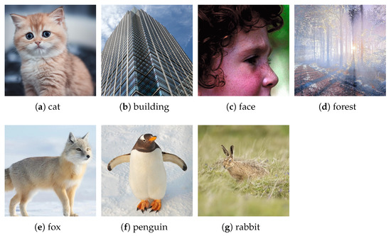
Figure 1. Ground-truth images.

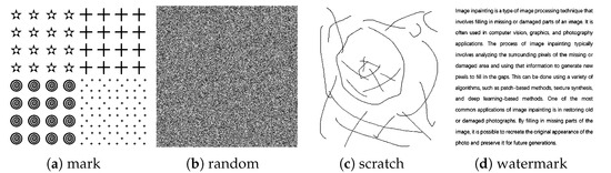
Figure 2. Mask images.

All experimental programs are coded in MATLAB R2023b and Python 3.11.8 under Windows 11 64-bit and run on a system equipped with a 3.70 GHz Intel Core i5-12600KF CPU and 32 GB of memory with GPU NVIDIA GeForce RTX 4070 12G and CUDA Version: 12.7.

4.1. Parameter Effect on Algorithms

The main computational part of our algorithm is Algorithm 1, in which the parameters $\alpha$ and p affect the algorithm results and the computing speed. To show which parameters $\alpha$ and p value will attain the best result, we take parameter $\alpha$ for every $0.1$ step in an open interval $(0,2)$ and parameter p in every $0.1$ step in a closed interval $[1,2]$ to experiment, using the image cat Figure 1a and mask Figure 2a to show the effect.

Using inequality (53), we show how n will change with an increase in the parameter $\alpha$ and the time to calculate $T_u\left(u\right)$ 100 times using Algorithm 1. The results showed in Table 1 tell that window size will increase when $\alpha <0.2$ and decrease when $\alpha >0.3$, and the computation time increases as n increases since the main computation in Algorithm 1 is convolved with an $n\times n$ matrix.

Table 1. Window size n and calculation time with a change in $\alpha$.

$\mathit{\alpha }$	${10}^{-9}$	0.1	0.15	0.2	0.3	0.4	0.5	0.6	0.7	0.8	0.9
n	1	67	42	84	81	73	63	54	46	40	34
Time (s)	0.19	13.78	19.08	4.17	20.06	16.33	12.20	9.02	6.58	1.01	3.65
$\alpha$	1.0	1.1	1.2	1.3	1.4	1.5	1.6	1.7	1.8	1.9	$2-{10}^{-9}$
n	30	26	23	20	17	15	13	11	9	7	1
Time (s)	2.87	2.18	1.73	0.31	0.99	0.79	0.62	0.47	0.35	10.25	0.19

Both $\alpha$ and p will affect the result in inpainting. To show what value of $\alpha$ and p will get the best result, we used image cat Figure 1a and mask mark Figure 2a and used Algorithm 2 for inpainting, using PSNR (56) to show the performance of the combination of these two parameters. The results are shown in Figure 3, where the rows represent the value of p and the columns represent the value of $\alpha$. We can see that the best result happened when $\alpha =1.5$ and $p=2$.

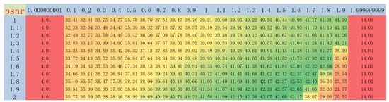
Figure 3. PSNR result with the change in $\alpha$ and p. PSNR values are color-coded from red (lowest: 14.01 dB) to green (highest: 42.68 dB), with intermediate values transitioning through yellow.

Furthermore, after conducting many experiments on various images and masks, the results have shown that the highest PSNR values are achieved when $1.3\le \alpha \le 1.7$ and $1.8\le p\le 2$. Meanwhile, while using our algorithm in image inpainting, we recommend choosing a small value for $\alpha$ when the mask is a thicker line.

4.2. Inpainting

This section presents the experimental results and relative analysis to demonstrate the effectiveness of our proposed image inpainting models. We compared our approach with several existing models, including traditional mathematical models, Total Variation (TV) [66], Total Generalized Variation (TGV) [67], Frequency Total Variation (ftTV) [68], and Adaptive modified Mumford–Shah Inpainting (AMSI) [69], and some deep learning models, Globally and Locally Consistent Image Completion (GLCIC) [70], Rethinking Image Inpainting via a Mutual Encoder–Decoder with Feature Equalizations (MEDFE) [71], and Aggregated Contextual Transformations for High-Resolution Image Inpainting (AOT-GAN) [72].

In the inpainting problem, masks are applied directly to ground-truth images that are assumed to be noise-free. The results of our model and those of Total Variation (TV) [66], Total Generalized Variation (TGV) [67], Adaptive modified Mumford–Shah Inpainting (AMSI) [69], Globally and Locally Consistent Image Completion (GLCIC) [70] and Aggregated Contextual Transformations for High-Resolution Image Inpainting (AOT-GAN) [72] models all had been shown in Figure 4, Figure 5, Figure 6, Figure 7, Figure 8, Figure 9, Figure 10, Figure 11, Figure 12, Figure 13, Figure 14, Figure 15, Figure 16, Figure 17, Figure 18, Figure 19, Figure 20, Figure 21, Figure 22, Figure 23, Figure 24, Figure 25, Figure 26, Figure 27, Figure 28, Figure 29, Figure 30 and Figure 31. To enhance the visual impact, we incorporated multiple color-coded boxes to highlight the details.

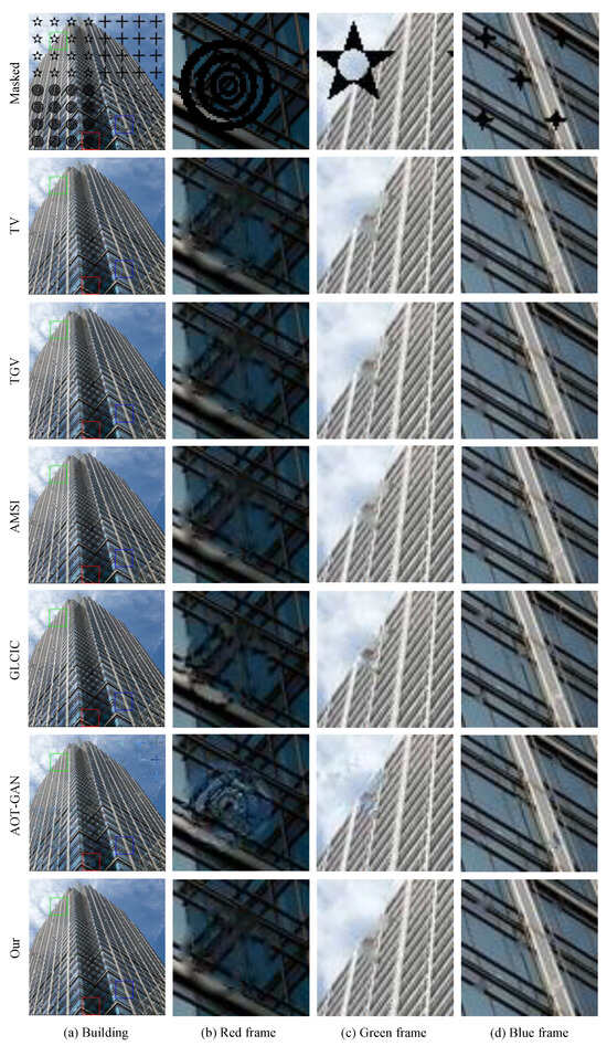
Figure 4. Examples of building image with mark recovery.

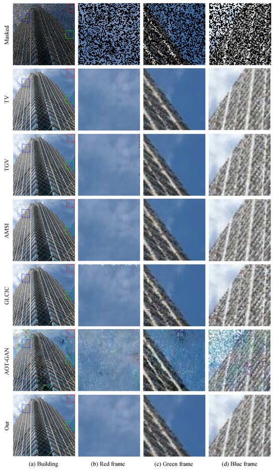
Figure 5. Examples of building image with random recovery.

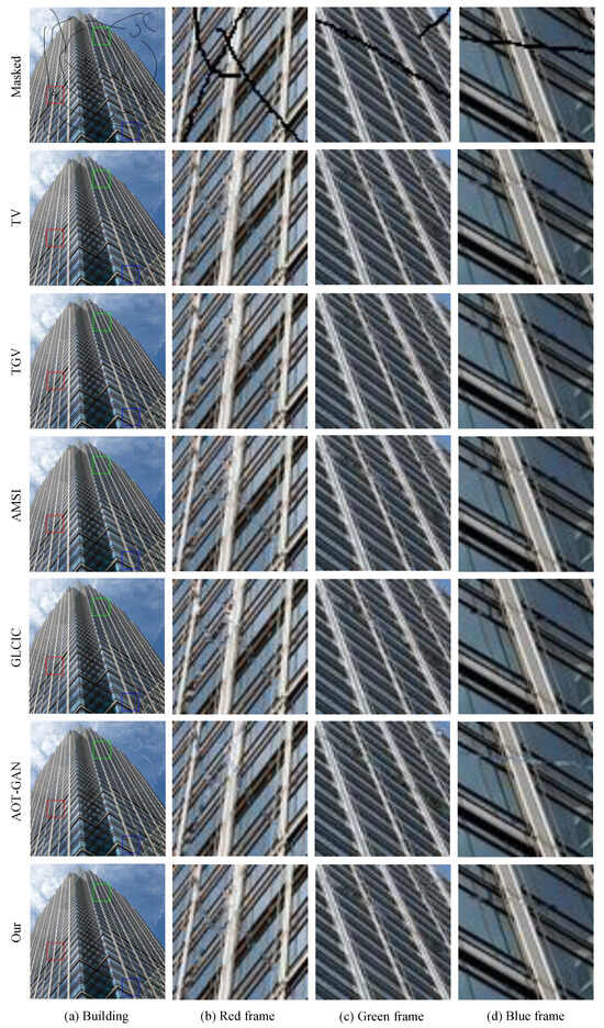
Figure 6. Examples of building image with scratch recovery.

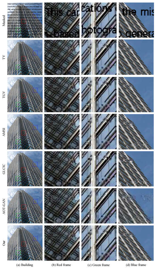
Figure 7. Examples of building image with watermark recovery.

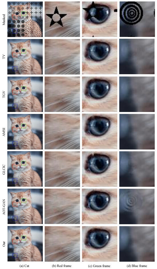
Figure 8. Examples of cat image with mark recovery.

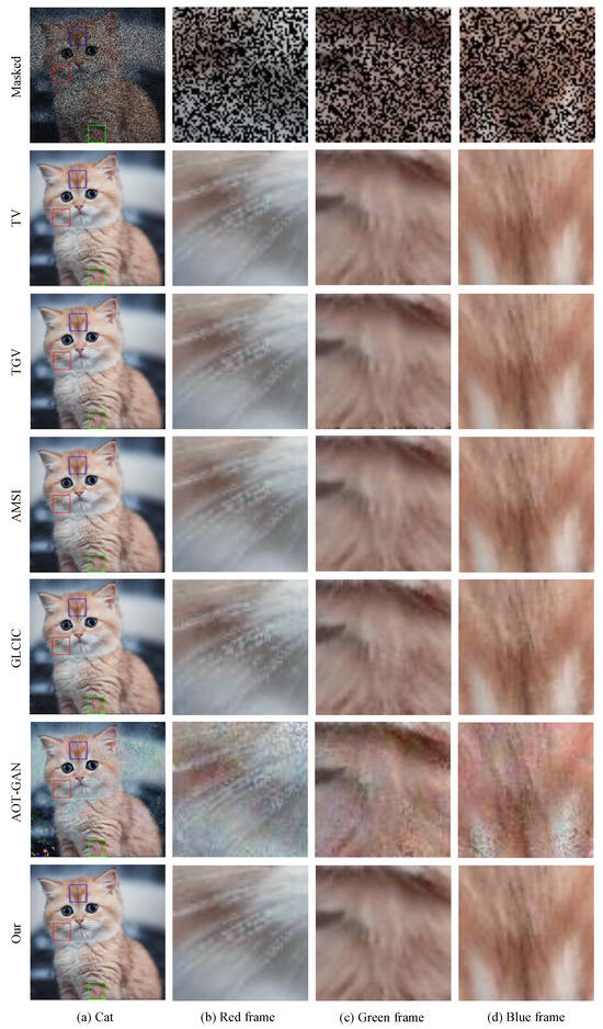
Figure 9. Examples of cat image with random recovery.

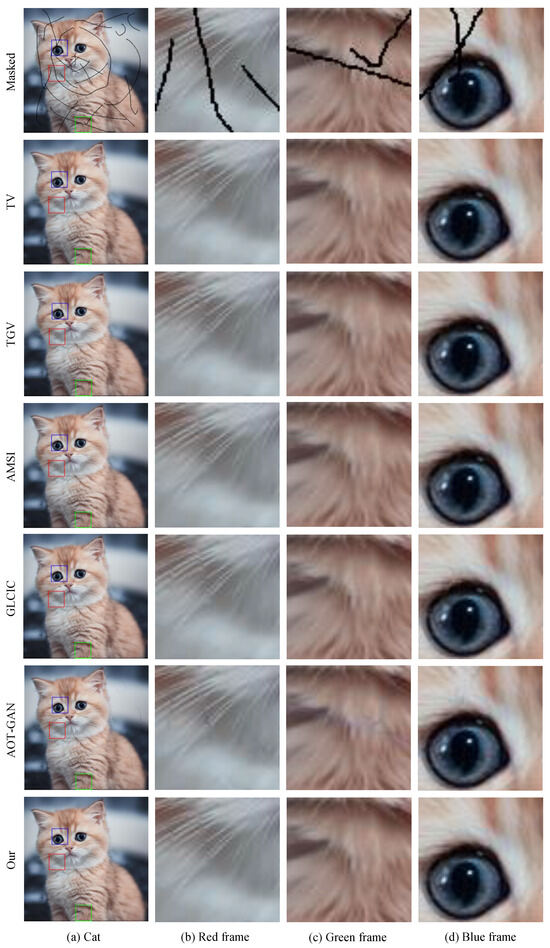
Figure 10. Examples of cat image with scratch recovery.

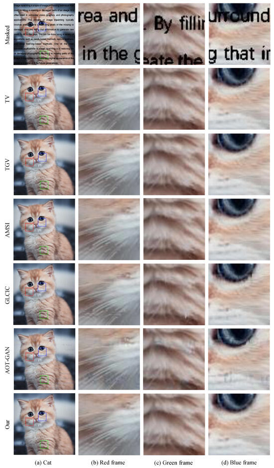
Figure 11. Examples of cat image with watermark recovery.

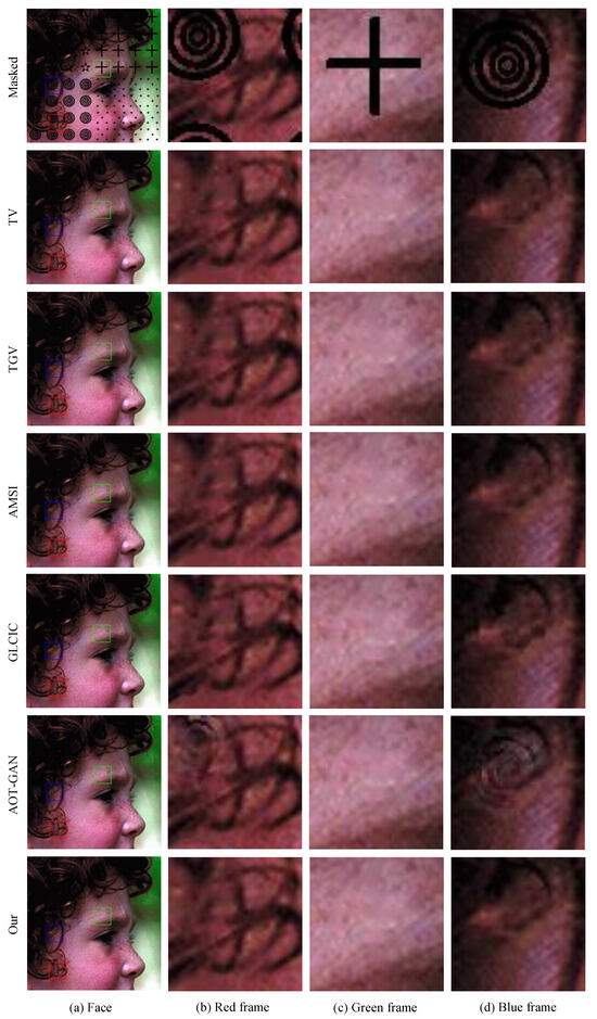
Figure 12. Examples of face image with mark recovery.

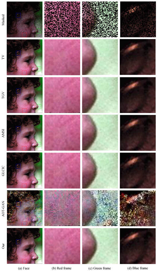
Figure 13. Examples of face image with random recovery.

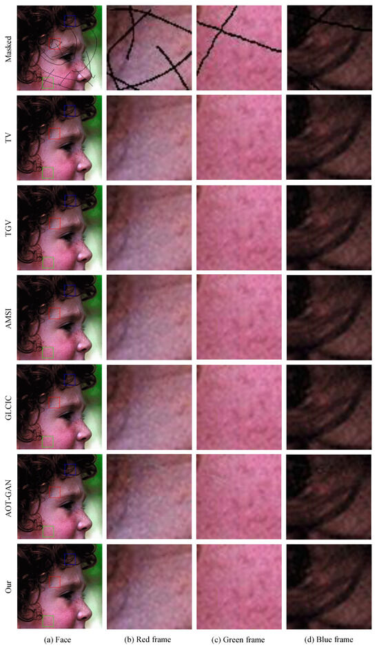
Figure 14. Examples of face image with scratch recovery.

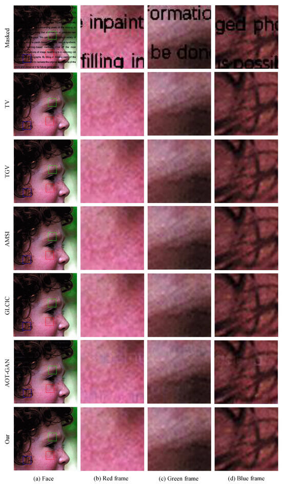
Figure 15. Examples of face image with watermark recovery.

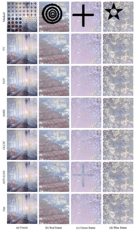
Figure 16. Examples of forest image with mark recovery.

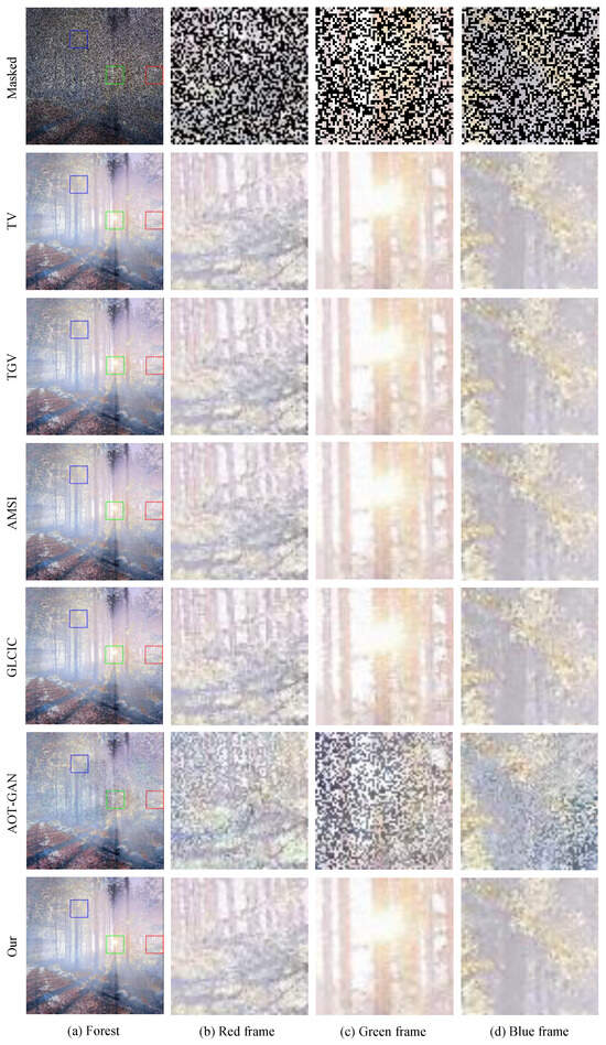
Figure 17. Examples of forest image with random recovery.

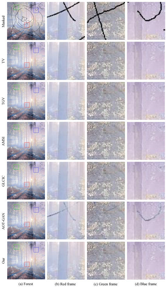
Figure 18. Examples of forest image with scratch recovery.

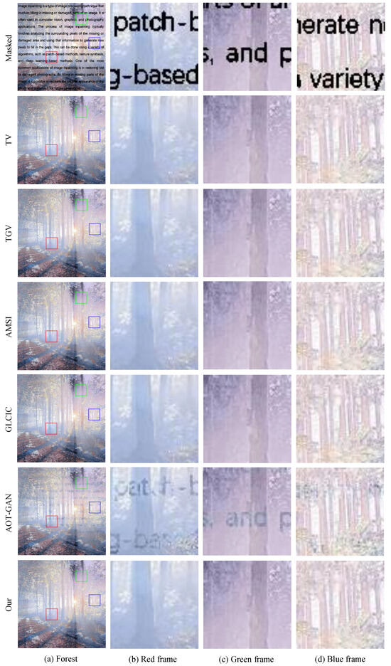
Figure 19. Examples of forest image with watermark recovery.

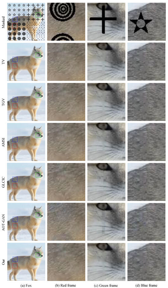
Figure 20. Examples of fox image with mark recovery.

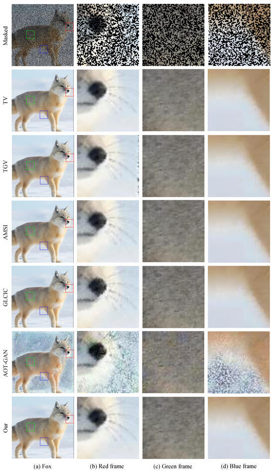
Figure 21. Examples of fox image with random recovery.

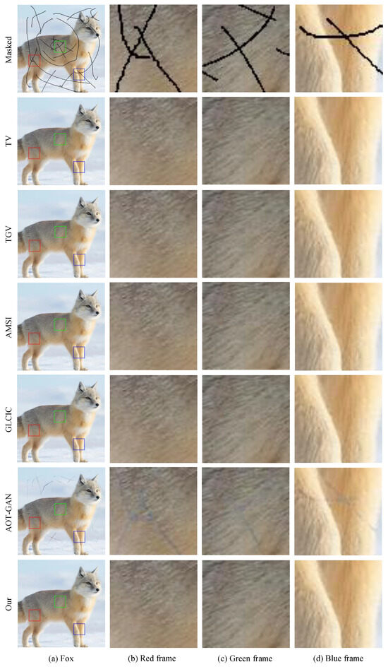
Figure 22. Examples of fox image with scratch recovery.

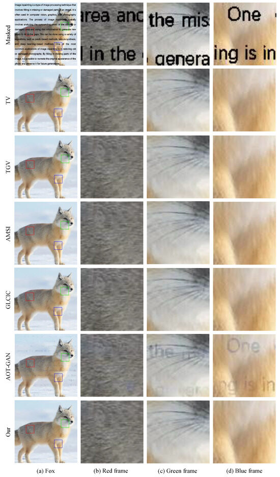
Figure 23. Examples of fox image with watermark recovery.

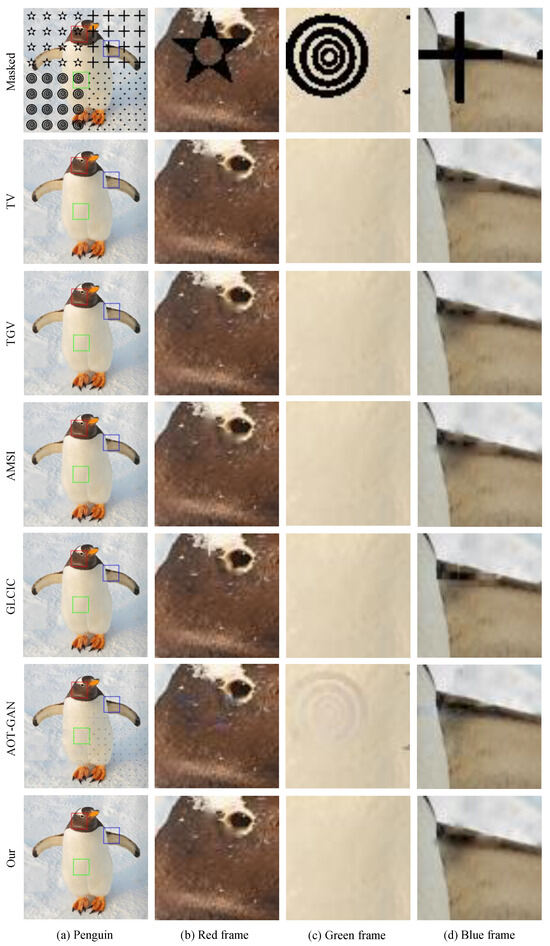
Figure 24. Examples of penguin image with mark recovery.

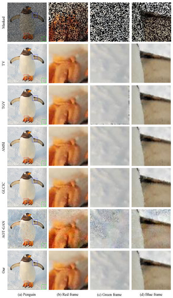
Figure 25. Examples of penguin image with random recovery.

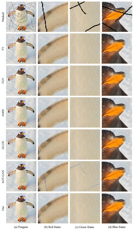
Figure 26. Examples of penguin image with scratch recovery.

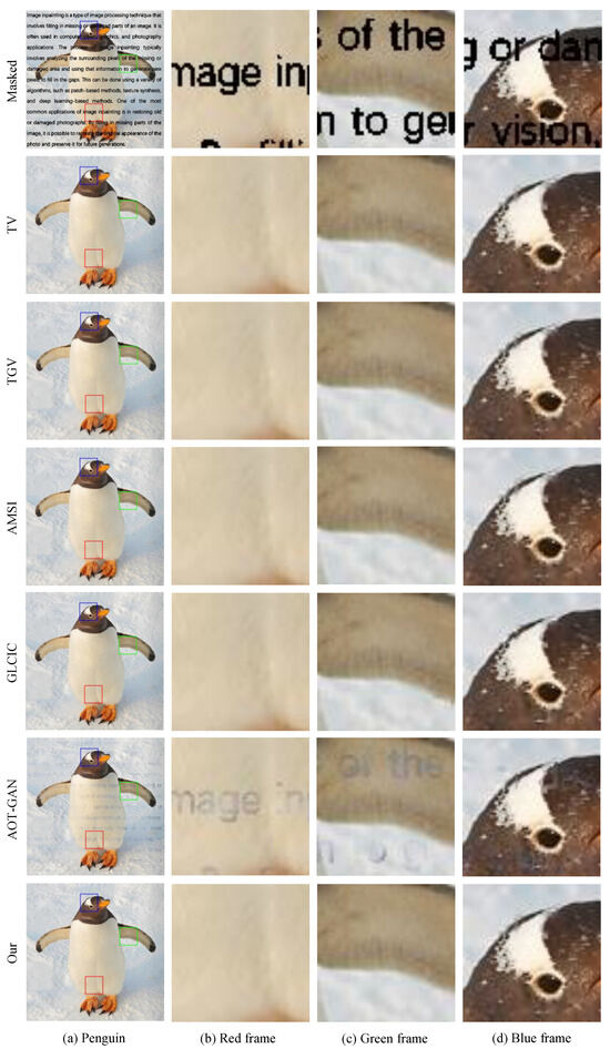
Figure 27. Examples of penguin image with watermark recovery.

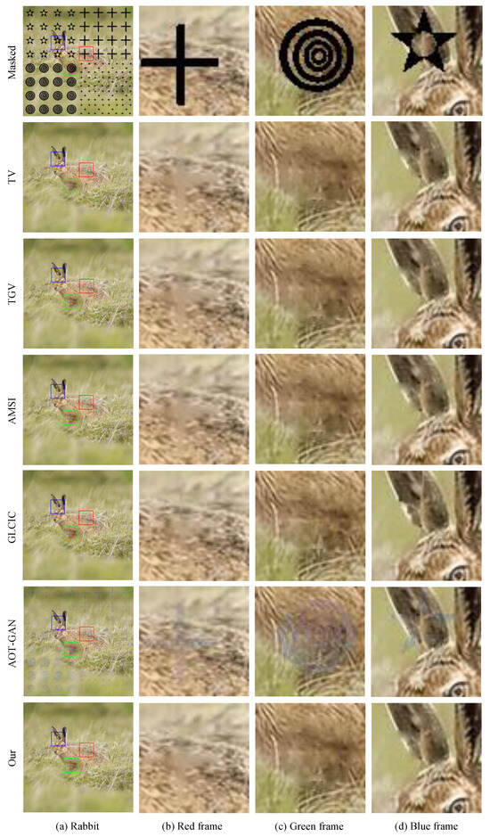
Figure 28. Examples of rabbit image with mark recovery.

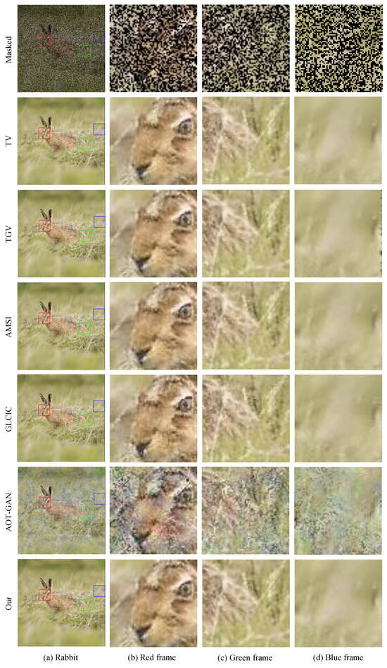
Figure 29. Examples of rabbit image with random recovery.

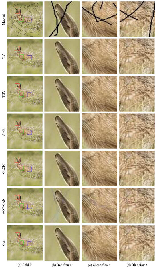
Figure 30. Examples of rabbit image with scratch recovery.

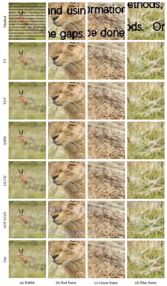
Figure 31. Examples of rabbit image with watermark recovery.

We can see that deep learning models are incapable of inpainting images from thin curve mask, and the random mask Figure 2b, will completely destroy the ability to recover. The advantage of deep learning models may be inpainting images from large areas of masks, because the traditional model cannot inpaint images when a large area of image information is missing; it needs to use the surrounding information to know what the pixel value is in the masked area.

We can clearly see in the cat masked mark in the Figure 8 that our model based on the Fractional Laplacian operator can recover the masked image on hair details better than other traditional models like Total Variation (TV) [66], Total Generalized Variation (TGV) [67], and Adaptive modified Mumford-Shah Inpainting (AMSI) [69]; meanwhile, those models cannot recover a random mask in the edge of the image. All the results on PSNR and SSIM are shown on Table 2.

Table 2. Image inpainting comparison results in terms of PSNR and SSIM.

		TV	TGV	ftTV	AMSI	GLCIC	MEDFE	AOT-GAN	Ours
Image	Mask
Building	Mark	24.59	24.38	24.66	24.66	23.43	18.20	23.73	24.69
		0.9409	0.9417	0.9424	0.9424	0.9344	0.6249	0.9358	0.9431
	Random	20.38	20.28	20.47	20.47	18.93	18.10	16.71	20.55
		0.8359	0.8434	0.8403	0.8403	0.7944	0.6124	0.6821	0.8422
	Scratch	31.57	31.41	31.63	31.63	30.60	18.32	29.95	31.71
		0.9884	0.9888	0.9887	0.9887	0.9864	0.6365	0.9806	0.9889
	Watermark	25.82	25.64	25.87	25.87	24.47	18.27	24.81	25.95
		0.9546	0.9561	0.9556	0.9556	0.9449	0.6315	0.9381	0.9565
Cat	Mark	41.20	42.04	41.85	41.85	39.71	32.37	34.51	42.73
		0.9925	0.9935	0.9940	0.9940	0.9907	0.9460	0.9662	0.9948
	Random	39.42	38.63	40.24	40.23	33.17	35.94	21.30	40.62
		0.9864	0.9839	0.9894	0.9894	0.9671	0.9753	0.6288	0.9900
	Scratch	49.18	49.81	50.06	50.06	47.89	37.03	39.43	50.41
		0.9985	0.9987	0.9988	0.9988	0.9981	0.9772	0.9851	0.9989
	Watermark	43.98	44.89	44.82	44.82	41.19	36.82	35.47	45.22
		0.9955	0.9962	0.9965	0.9965	0.9936	0.9767	0.9608	0.9967
Face	Mark	39.22	39.77	39.96	39.96	38.43	31.54	34.75	40.21
		0.9882	0.9895	0.9901	0.9901	0.9850	0.9239	0.9649	0.9905
	Random	36.67	36.05	38.13	38.13	30.81	33.46	14.51	38.88
		0.9750	0.9758	0.9826	0.9826	0.9500	0.9419	0.4029	0.9844
	Scratch	47.56	48.27	48.80	48.80	46.82	34.53	39.20	49.55
		0.9982	0.9985	0.9987	0.9987	0.9979	0.9552	0.9810	0.9988
	Watermark	41.01	41.85	42.16	42.17	39.91	34.31	33.45	42.70
		0.9914	0.9927	0.9934	0.9934	0.9877	0.9526	0.9374	0.9940
Forest	Mark	30.52	30.42	30.51	30.51	29.44	23.35	27.80	30.58
		0.9488	0.9495	0.9496	0.9496	0.9434	0.6290	0.9155	0.9489
	Random	25.92	25.70	25.92	25.92	24.62	23.74	18.71	25.94
		0.8370	0.8348	0.8382	0.8381	0.8000	0.6405	0.5602	0.8361
	Scratch	37.59	37.43	37.58	37.58	36.57	23.89	32.94	37.63
		0.9899	0.9897	0.9898	0.9898	0.9880	0.6553	0.9699	0.9898
	Watermark	31.33	31.27	31.32	31.32	30.23	23.86	26.93	31.35
		0.9559	0.9564	0.9563	0.9563	0.9486	0.6520	0.8901	0.9560
Fox	Mark	41.07	41.26	41.24	41.24	39.54	31.16	35.10	41.34
		0.9893	0.9898	0.9901	0.9901	0.9876	0.9107	0.9653	0.9902
	Random	36.90	34.10	37.23	37.22	34.71	34.21	16.75	36.96
		0.9698	0.9610	0.9730	0.9730	0.9581	0.9389	0.5147	0.9731
	Scratch	48.04	48.05	48.51	48.51	47.00	34.62	35.07	48.63
		0.9976	0.9977	0.9979	0.9979	0.9974	0.9416	0.9738	0.9979
	Watermark	41.61	42.01	41.98	41.98	40.02	34.56	32.69	42.19
		0.9913	0.9919	0.9924	0.9924	0.9901	0.9410	0.9437	0.9925
Penguin	Mark	39.08	40.12	39.48	39.48	37.94	30.10	33.38	40.45
		0.9898	0.9912	0.9925	0.9925	0.9895	0.9208	0.9424	0.9935
	Random	37.18	34.80	37.48	37.48	34.37	33.22	19.25	37.60
		0.9808	0.9708	0.9882	0.9882	0.9676	0.9633	0.4581	0.9897
	Scratch	46.34	46.43	46.61	46.61	45.71	34.33	38.20	46.93
		0.9985	0.9986	0.9990	0.9990	0.9982	0.9733	0.9774	0.9991
	Watermark	42.13	42.76	42.42	42.42	40.12	34.12	31.85	43.12
		0.9933	0.9941	0.9955	0.9955	0.9920	0.9708	0.9073	0.9962
Rabbit	Mark	37.88	38.31	38.35	38.35	37.03	29.56	31.26	38.38
		0.9951	0.9956	0.9957	0.9957	0.9948	0.9634	0.9662	0.9958
	Random	33.10	32.92	33.74	33.74	30.73	30.49	20.03	33.82
		0.9849	0.9845	0.9873	0.9873	0.9761	0.9703	0.6611	0.9882
	Scratch	43.00	43.59	43.53	43.53	42.38	30.62	36.07	43.79
		0.9986	0.9988	0.9988	0.9988	0.9985	0.9701	0.9885	0.9989
	Watermark	38.25	38.84	38.83	38.83	37.35	30.58	29.59	39.01
		0.9955	0.9961	0.9962	0.9962	0.9951	0.9701	0.9461	0.9964

Note: Bold numbers indicate the best PSNR and SSIM values in each row.

4.3. Comparison of Calculation Time

In practical applications, in addition to the inpainting result, the time required for inpainting is also an indicator for evaluating the algorithm’s superiority. For traditional algorithms, most algorithms require many iterations of computation, while deep learning algorithms generally need a short processing time through the neural network. However, in reality, the most time-consuming part of deep learning methods is during the training phase, sometimes taking several hours, days, or even weeks. The time required to process a single image is related to the mask, and the results are shown in Table 3.

Table 3. Image inpainting comparison results in terms of time.

Time (s)	TV	TGV	ftTV	AMSI	GLCIC	MEDFE	AOT-GAN	Our
Mark	7.868	203.646	6.865	35.524	0.549	0.122	1.101	44.721
Random	5.722	171.770	4.785	31.137	15.692	0.061	1.099	15.175
Scratch	4.395	138.177	3.948	34.716	0.611	0.061	1.098	12.106
Watermark	5.556	166.638	4.710	35.190	0.795	0.065	1.096	17.969

The computational time of the deep learning method is much lower than the traditional mathematical models, but if we consider the training time, traditional models still have significant advantages.

4.4. Inpainting and Denoising

To show the ability in inpainting and denoising of our model, we add some different types of noise to all images in Figure 1. We use seven kinds of noise as follows:

• Exponential Noise: The probability distribution function of exponential noise is

  $$p\left(z\right)=\left\{\begin{array}{cc}\lambda e^{-\lambda z},\hfill & z\ge 0;\hfill \\ 0,\hfill & z<0.\hfill \end{array}\right.$$
• Gamma Noise: The probability distribution function of gamma noise is

  $$p\left(z\right)=\left\{\begin{array}{cc}{\displaystyle \frac{{\lambda }^k{z}^{k-1}{e}^{-\lambda z}}{(k-1)!}},\hfill & z\ge 0;\hfill \\ 0,\hfill & z<0.\hfill \end{array}\right.$$
• Gaussian Noise: The probability distribution function of Gaussian noise is

  $$p\left(z\right)={\displaystyle \frac{1}{\sqrt{2\pi {\sigma }^2}}}{e}^{-{\displaystyle \frac{{(z-\mu )}^2}{2{\sigma }^2}}}.$$
• Poisson Noise: The probability distribution function of Poisson noise is:

  $$P\left(k\right)={\displaystyle \frac{{\lambda }^k{e}^{-\lambda }}{k!}}.$$
• Rayleigh Noise: The probability distribution function of Rayleigh noise is

  $$p\left(z\right)=\left\{\begin{array}{cc}{\displaystyle \frac{z}{{\sigma }^2}}{e}^{-z^2/\left(2{\sigma }^2\right)},\hfill & z\ge 0;\hfill \\ 0,\hfill & z<0.\hfill \end{array}\right.$$
• Salt-and-Pepper Noise: The probability distribution function of salt-and-pepper noise is

  $$I(x,y)=\left\{\begin{array}{cc}0,\hfill & \mathrm{with}\mathrm{probability}{p}_{\mathrm{pepper}};\hfill \\ 255,\hfill & \mathrm{with}\mathrm{probability}{p}_{\mathrm{salt}};\hfill \\ I_0(x,y),\hfill & \mathrm{with}\mathrm{probability}1-p_{\mathrm{pepper}}-p_{\mathrm{salt}}.\hfill \end{array}\right.$$
• Uniform Noise: The probability distribution function of uniform noise is

  $$p\left(z\right)=\left\{\begin{array}{cc}{\displaystyle \frac{1}{b-a}},\hfill & a\le z\le b;\hfill \\ 0,\hfill & \mathrm{otherwise}.\hfill \end{array}\right.$$

Table 4 shows the PSNR and SSIM results of Algorithm 3 in inpainting and denoising. Figure 32, Figure 33, Figure 34, Figure 35, Figure 36, Figure 37, Figure 38, Figure 39, Figure 40, Figure 41, Figure 42 and Figure 43 show the recovered noised image in using $H^{-1}$ norm. We have the same result with Osher [43] that using $H^{-1}$ norm instead of $L^2$ norm can have a better result in inpainting and denoising. It shows that our method can recover the destroyed image and reduce noise at the same time.

Table 4. Inpainting results for images with denoising in additive noise.

Exponential Noise	Mark	Random	Scratch	Watermark
Building	23.5219 0.9194	20.1381 0.8180	27.4947 0.9631	24.2992 0.9260
Cat	31.3146 0.9546	30.5670 0.8946	31.4633 0.9561	31.2976 0.9601
Face	30.8266 0.9121	30.5651 0.8991	31.1467 0.9190	30.9665 0.9139
Forest	26.6060 0.8831	24.4644 0.7803	24.7045 0.9017	24.4132 0.8687
Fox	30.3924 0.9374	30.7804 0.9306	30.8616 0.9489	30.5092 0.9463
Penguin	30.5294 0.9402	30.7373 0.9271	30.7464 0.9524	30.8528 0.9482
Rabbit	30.0392 0.9835	29.2628 0.9733	30.4775 0.9856	30.2554 0.9831
Gamma Noise	Mark	Random	Scratch	Watermark
Building	23.5345 0.9191	20.1374 0.8177	27.4883 0.9629	24.3454 0.9278
Cat	31.0909 0.9550	30.8529 0.9153	31.5462 0.9569	31.2054 0.9599
Face	30.8984 0.9125	30.5897 0.8991	31.2104 0.9195	30.9707 0.9141
Forest	26.7144 0.8839	24.4632 0.7803	24.8728 0.9033	25.8153 0.8861
Fox	30.3399 0.9371	30.6962 0.9318	31.0956 0.9463	30.4271 0.9445
Penguin	30.3736 0.9402	30.0680 0.9407	30.5794 0.9512	30.8383 0.9485
Rabbit	30.0301 0.9834	29.2411 0.9735	30.4779 0.9855	30.2499 0.9831
Poisson noise	Mark	Random	Scratch	Watermark
Building	23.0979 0.8803	20.0634 0.7957	26.3553 0.9218	23.9323 0.8941
Cat	32.3407 0.8950	30.0989 0.8327	32.6814 0.8973	33.1093 0.9077
Face	34.1826 0.9593	33.1467 0.9480	35.2935 0.9677	34.4262 0.9620
Forest	26.0793 0.7895	24.3409 0.7113	27.1964 0.8167	26.2036 0.7885
Fox	32.6150 0.9036	31.3355 0.8669	32.3688 0.8871	31.6808 0.8722
Penguin	31.4094 0.8124	31.2699 0.8321	32.1187 0.8392	32.0490 0.8556
Rabbit	30.6436 0.9665	29.0811 0.9536	30.9963 0.9681	30.6285 0.9663
Rayleigh Noise	Mark	Random	Scratch	Watermark
Building	22.0915 0.9075	19.2451 0.7863	23.8002 0.9451	22.0345 0.9029
Cat	26.1147 0.9420	26.2009 0.8374	25.9137 0.9446	25.7753 0.9302
Face	25.9880 0.8552	26.2727 0.8352	25.8990 0.8602	26.0377 0.8520
Forest	23.5722 0.8684	20.9930 0.7091	20.3927 0.8348	20.2043 0.7962
Fox	25.3740 0.9284	26.7237 0.9003	25.5398 0.9386	25.3137 0.9317
Penguin	25.7521 0.9295	26.8164 0.8680	25.6746 0.9465	26.0382 0.9304
Rabbit	25.6232 0.9793	25.6816 0.9656	25.5858 0.9772	25.8484 0.9772
Salt-and-Pepper Noise	Mark	Random	Scratch	Watermark
Building	23.7426 0.9245	20.2712 0.8300	27.9141 0.9690	24.7012 0.9385
Cat	35.1192 0.9645	33.1050 0.9574	35.9147 0.9675	35.4334 0.9653
Face	34.2389 0.9563	33.5288 0.9552	35.4364 0.9650	34.4533 0.9589
Forest	27.4748 0.8913	25.1746 0.8000	29.4569 0.9343	28.0936 0.9091
Fox	33.7617 0.9350	33.3341 0.9375	34.6032 0.9487	34.1221 0.9484
Penguin	33.8500 0.9537	33.1736 0.9554	34.3207 0.9584	33.9043 0.9584
Rabbit	32.7510 0.9827	31.0736 0.9756	33.7107 0.9858	32.9432 0.9833
Uniform Noise	Mark	Random	Scratch	Watermark
Building	24.1427 0.9232	20.3883 0.8276	29.3024 0.9678	25.2204 0.9366
Cat	36.2064 0.9609	33.7892 0.9299	36.7609 0.9615	36.9413 0.9657
Face	35.2313 0.9574	34.4223 0.9449	36.8067 0.9655	35.7369 0.9597
Forest	28.5367 0.8953	25.4301 0.7935	31.4508 0.9361	29.1955 0.9059
Fox	34.3727 0.9396	34.1130 0.9350	35.6981 0.9513	35.3842 0.9494
Penguin	34.9857 0.9465	33.8864 0.9462	35.8017 0.9582	34.9193 0.9567
Rabbit	33.7146 0.9855	31.5987 0.9765	34.5199 0.9875	33.6418 0.9851

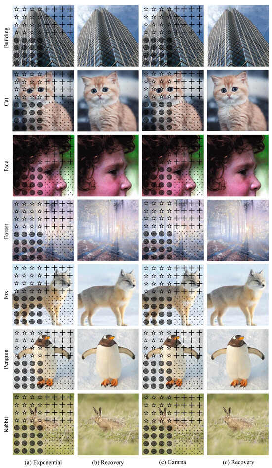
Figure 32. Examples of image inpainting and denoising with mask mark in exponential noise and Gamma noise.

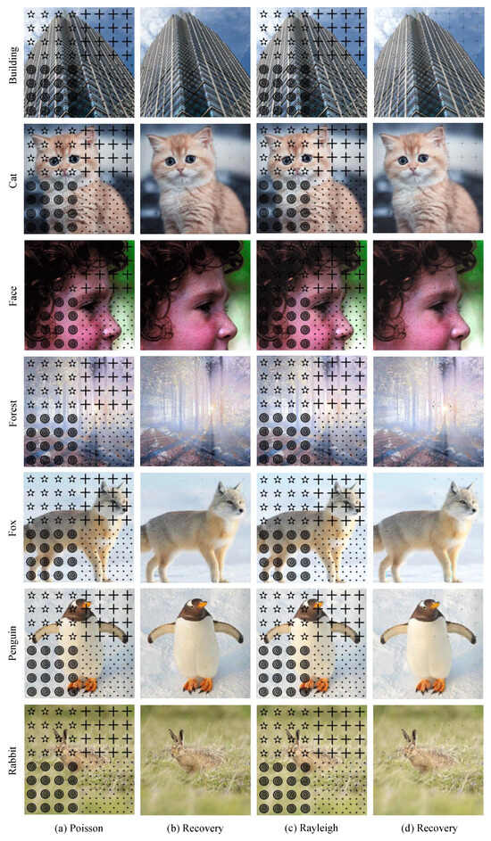
Figure 33. Examples of image inpainting and denoising with mask mark in Poisson noise and Rayleigh noise.

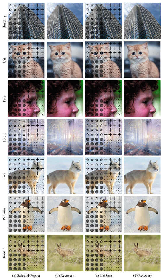
Figure 34. Examples of image inpainting and denoising with mask mark in salt-and-pepper noise and uniform noise.

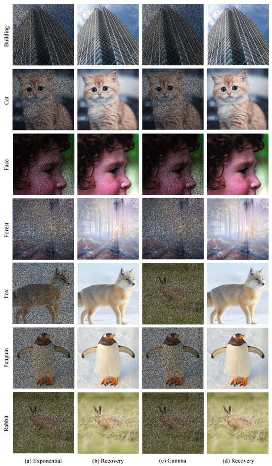
Figure 35. Examples of image inpainting and denoising with mask random in exponential noise and Gamma noise.

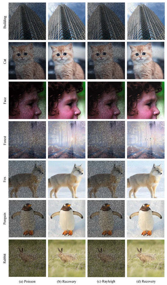
Figure 36. Examples of image inpainting and denoising with mask random in Poisson noise and Rayleigh noise.

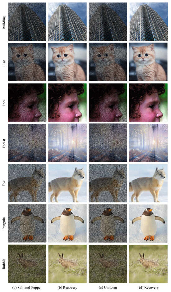
Figure 37. Examples of image inpainting and denoising with mask random in salt-and-pepper noise and uniform noise.

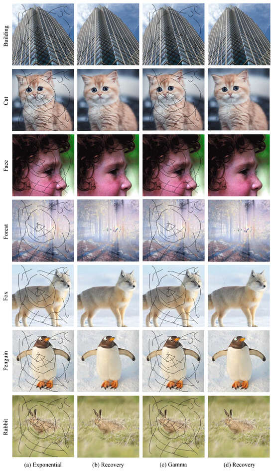
Figure 38. Examples of image inpainting and denoising with mask scratch in exponential noise and Gamma noise.

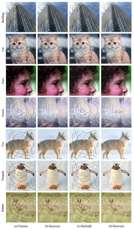
Figure 39. Examples of image inpainting and denoising with mask scratch in Poisson noise and Rayleigh noise.

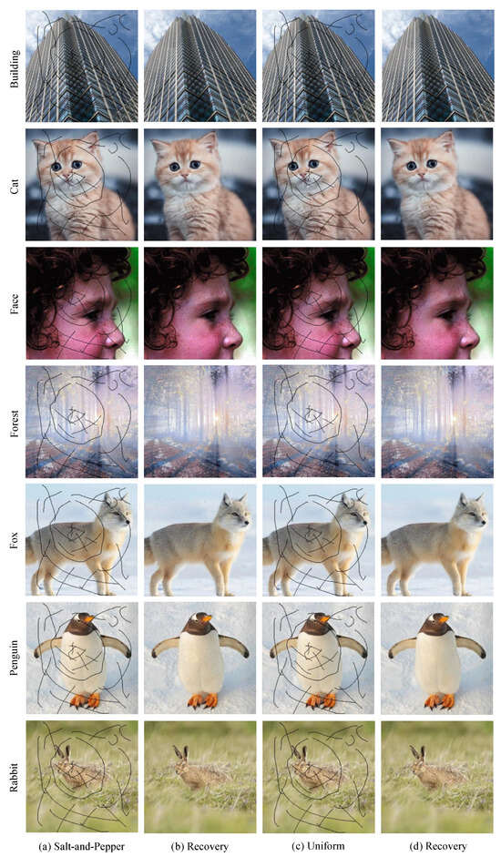
Figure 40. Examples of image inpainting and denoising with mask scratch in salt-and-pepper noise and uniform noise.

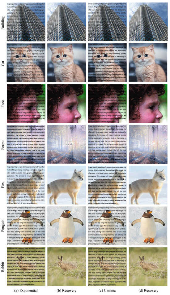
Figure 41. Examples of image inpainting and denoising with mask watermark in exponential noise and Gamma noise.

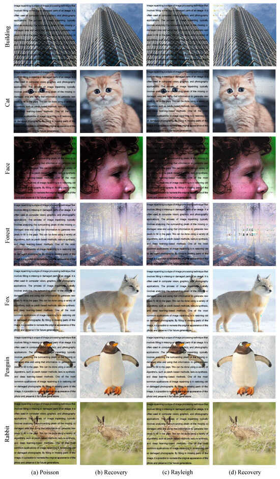
Figure 42. Examples of image inpainting and denoising with mask watermark in Poisson noise and Rayleigh noise.

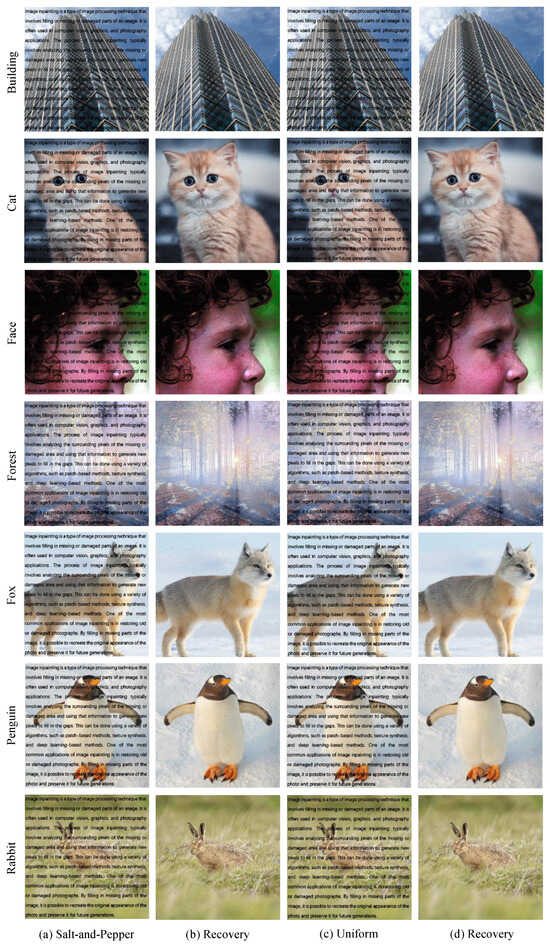
Figure 43. Examples of image inpainting and denoising with mask watermark in salt-and-pepper noise and uniform noise.

In Figure 40, we can see the noise has been reduced and mask area has been repaired. The effect of our algorithm can be seen easily.

We observed that $H^{-1}$ norm can better separate oscillatory components from high-frequency components compared to the $L^2$ norm, while also being better at removing noise while preserving edges. To show that this improvement can bring a better result, we add Gaussian noise with mean $\mu =0$, standard deviation $\sigma =8$, and $\sigma =36$ to all images in Figure 1. Table 5 and Table 6 show the PSNR and SSIM results of Algorithm 3, comparing $H^{-1}$ norm with $L^2$ norm in inpainting and denoising. Figure 44, Figure 45, Figure 46 and Figure 47 show the recovered noised image in using $H^{-1}$ norm. We have the same result with Osher [43] that using the $H^{-1}$ norm instead of the $L^2$ norm can have a better result in inpainting and denoising. It shows that our method can recover the destroyed image and reduce noise at the same time.

Table 5. Norm $H^{-1}$ and $L^2$ comparison in inpainting and denoising with standard deviation $\sigma =8$.

Image	$\mathit{\sigma }=8$	Mark	Random	Scratch	Watermark
Building	$H^{-1}$	23.5013 0.9003	20.1948 0.8115	27.3354 0.9430	24.4183 0.9141
	$L^2$	19.0140 0.7072	17.9458 0.6146	20.6456 0.8922	19.2468 0.7158
Cat	$H^{-1}$	34.1832 0.9287	32.0829 0.8827	34.7117 0.9316	34.9303 0.9386
	$L^2$	33.2248 0.9413	26.2452 0.8865	33.7216 0.9338	31.1999 0.9358
Face	$H^{-1}$	34.0763 0.9382	33.0326 0.9189	35.1232 0.9451	34.2459 0.9382
	$L^2$	33.8527 0.9334	32.7048 0.9077	33.3967 0.9112	33.1220 0.9095
Forest	$H^{-1}$	27.5368 0.8575	25.0017 0.7635	29.4249 0.8916	27.8671 0.8614
	$L^2$	22.8940 0.5629	23.1994 0.5984	23.4636 0.6089	23.8516 0.6505
Fox	$H^{-1}$	33.7629 0.9287	32.9811 0.9125	34.3072 0.9302	33.8023 0.9237
	$L^2$	34.1767 0.9322	33.0466 0.9171	32.9092 0.8976	33.6286 0.9184
Penguin	$H^{-1}$	33.5357 0.9003	32.8536 0.9074	34.6136 0.9187	34.0214 0.9232
	$L^2$	33.5320 0.9058	32.7783 0.8876	33.6433 0.8640	33.7135 0.8840
Rabbit	$H^{-1}$	32.1686 0.9775	30.3236 0.9666	32.6918 0.9793	32.1175 0.9771
	$L^2$	31.3957 0.9751	30.1936 0.9671	32.1703 0.9755	31.9561 0.9766

Table 6. Norm $H^{-1}$ and $L^2$ comparison in inpainting and denoising with standard deviation $\sigma =36$.

Image	$\mathit{\sigma }=36$	Mark	Random	Scratch	Watermark
Building	$H^{-1}$	18.7108 0.6828	17.7757 0.6074	19.4323 0.7166	18.9695 0.6944
	$L^2$	18.2491 0.6327	17.3849 0.5510	18.9258 0.6748	18.4319 0.6406
Cat	$H^{-1}$	28.3353 0.8140	25.9881 0.7903	28.0589 0.7944	29.1774 0.8496
	$L^2$	25.3165 0.6375	25.2741 0.6480	24.2393 0.5773	26.1413 0.6769
Face	$H^{-1}$	26.6930 0.7640	25.0878 0.6956	26.6180 0.7679	25.7667 0.7324
	$L^2$	24.2351 0.6294	22.0929 0.5284	21.4625 0.4956	21.5980 0.5028
Forest	$H^{-1}$	22.5199 0.5496	22.2628 0.5150	22.6790 0.5607	22.5657 0.5521
	$L^2$	22.5861 0.5406	22.3767 0.5265	22.8957 0.5670	22.9009 0.5713
Fox	$H^{-1}$	27.6064 0.8030	27.3667 0.7853	27.0020 0.7763	26.6973 0.7511
	$L^2$	24.7721 0.6116	25.3076 0.6448	21.3783 0.4194	23.2889 0.5236
Penguin	$H^{-1}$	27.2103 0.7281	26.1111 0.6589	27.9634 0.7501	27.0132 0.6988
	$L^2$	24.5030 0.4801	23.5745 0.4362	21.9900 0.3493	23.3234 0.4132
Rabbit	$H^{-1}$	26.0637 0.9118	25.2335 0.9048	25.9572 0.9084	26.1536 0.9168
	$L^2$	24.4858 0.8689	22.7802 0.8154	20.7357 0.7262	22.6686 0.8075

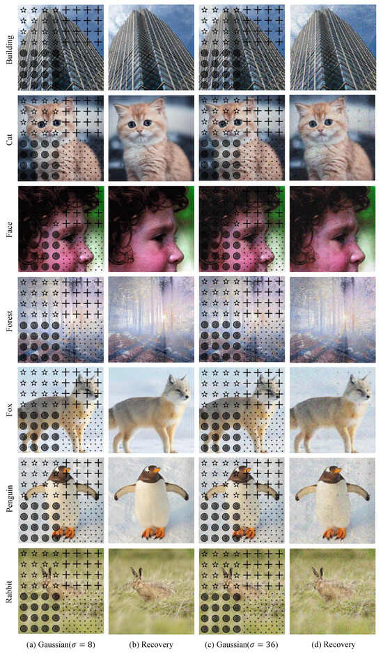
Figure 44. Examples of image inpainting and denoising with mask mark in Gaussian noise.

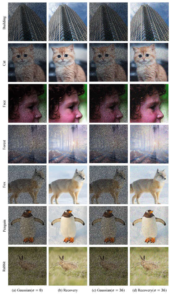
Figure 45. Examples of image inpainting and denoising with mask random in Gaussian noise.

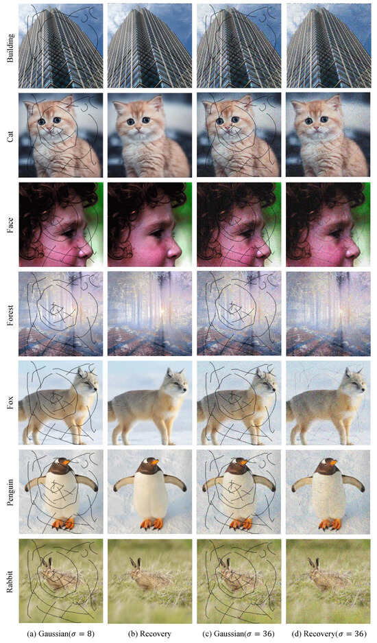
Figure 46. Examples of image inpainting and denoising with mask scratch in Gaussian noise.

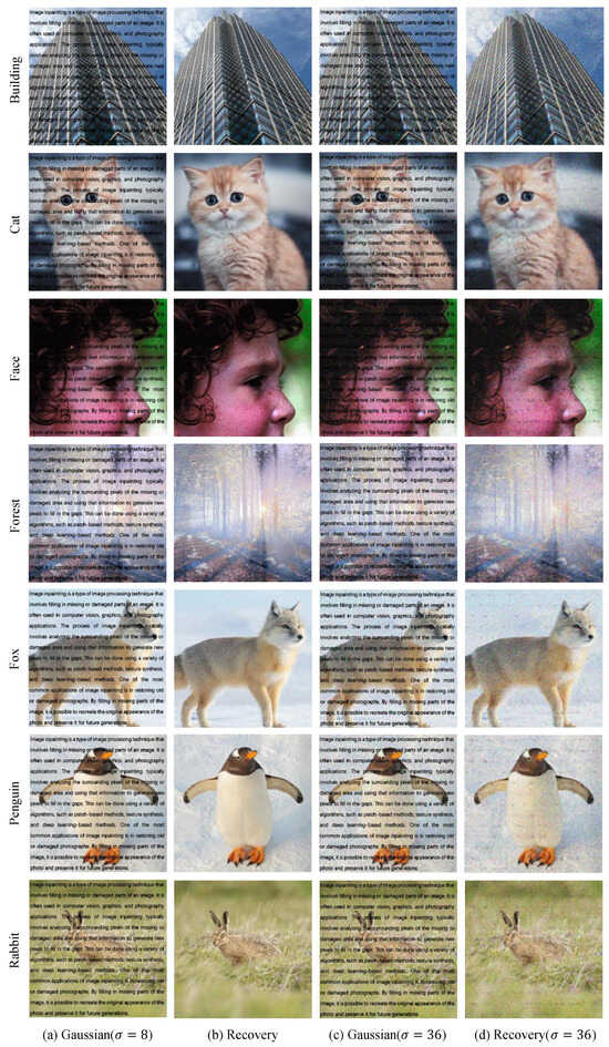
Figure 47. Examples of image inpainting and denoising with mask watermark in Gaussian noise.

5. Discussion

In this paper, we present an improved model based on the fractional Laplacian operator, which employs the $L^p$ norm of the fractional Laplacian operator as a regularization term and the $H^{-1}$ norm as a fidelity term; these improvements lead to better results in restoring damaged regions. The introduction of an intermediate variable to the diffusion equations resolves the difficulty in handling $H^{-1}$ term.

However, in the theoretical proof process, it is noted that the fractional Bessel potential space with $p=1$ is not a Banach space under the same norm definition, nor is it reflexive or separable. Since relevant theoretical research in this area is still ongoing, we have not extended our existence and uniqueness theorem to the case of $p=1$. Consistently, our experiments demonstrate that $p=1$ as a parameter for image inpainting yields unsatisfactory performance. Given that the constraint at $p=1$ induces sparse solutions, there may be some special cases where better outcomes could be achieved. Therefore, future work should specifically investigate whether similar results hold for $p=1$.

Model analysis confirms that our method is both theoretically sound and effective, with guaranteed convergence to the solution. Comparative experiments show that it consistently outperforms traditional models in preserving texture details and surpasses deep learning approaches in recovering thin curve masks. To further improve performance, we propose three potential strategies: (1) replacing deep learning methods with our approach for solving the diffusion equation, (2) using our energy functional as the loss function for network training, and (3) designing a hybrid pipeline where deep models handle large missing regions and our method refines fine structures. Such a combination strategy significantly enhances inpainting quality.

6. Conclusions

This paper proposes a novel image inpainting framework based on minimizing an energy functional that integrates an $L^p$-norm regularization term involving fractional-order Laplacian operators with an $H^{-1}$-norm fidelity term. The model is theoretically grounded via an associated diffusion equation whose solution converges to the variational minimizer, with convergence rigorously justified. A finite difference-based numerical scheme is derived from the diffusion formulation and is systematically evaluated through comprehensive experiments. Comparative studies against classical variational methods and deep learning models demonstrate the proposed method’s superior performance in preserving structural details and suppressing noise under various degradation scenarios.

References

- Bertalmio, M.; Sapiro, G.; Caselles, V.; Ballester, C. Image Inpainting. In Proceedings of the 27th Annual Conference on Computer Graphics and Interactive Techniques, New Orleans, LA, USA, 23–28 July 2000; pp. 417–424. [Google Scholar]
- Perona, P.; Malik, J. Scale-space and Edge Detection Using Anisotropic Diffusion. IEEE Trans. Pattern Anal. Mach. Intell. 1990, 12, 629–639. [Google Scholar] [CrossRef]
- Catté, F.; Lions, P.L.; Morel, J.M.; Coll, T. Image Selective Smoothing and Edge Detection by Nonlinear Diffusion. SIAM J. Numer. Anal. 1992, 29, 182–193. [Google Scholar] [CrossRef]
- Chan, T.F.; Shen, J. Variational Image Inpainting. Commun. Pure Appl. Math. J. Issued Courant Inst. Math. Sci. 2005, 58, 579–619. [Google Scholar] [CrossRef]
- Fadili, M.J.; Starck, J.L.; Murtagh, F. Inpainting and Zooming Using Sparse Representations. Comput. J. 2009, 52, 64–79. [Google Scholar] [CrossRef]
- Lysaker, M.; Lundervold, A.; Tai, X.C. Noise Removal Using Fourth-order Partial Differential Equation with Applications to Medical Magnetic Resonance Images in Space and Time. IEEE Trans. Image Process. 2003, 12, 1579–1590. [Google Scholar] [CrossRef]
- Kim, S.; Lim, H. Fourth-order Partial Differential Equations for Effective Image Denoising. Electron. J. Differ. Equ. (EJDE) 2009, 2009, 107–121. [Google Scholar]
- Zhao, D.H. Adaptive Fourth Order Partial Differential Equation Filter From the Webers Total Variation for Image Restoration. Appl. Mech. Mater. 2014, 475, 394–400. [Google Scholar] [CrossRef]
- Bai, J.; Feng, X.C. Fractional-order Anisotropic Diffusion for Image Denoising. IEEE Trans. Image Process. 2007, 16, 2492–2502. [Google Scholar] [CrossRef]
- Zhang, Y.; Pu, Y.F.; Hu, J.R.; Liu, Y.; Chen, Q.L.; Zhou, J.L. Efficient CT Metal Artifact Reduction Based on Fractional-order Curvature Diffusion. Comput. Math. Methods Med. 2011, 2011, 173748. [Google Scholar] [CrossRef]
- Chen, D.; Chen, Y.; Xue, D. Fractional-order total variation image restoration based on primal-dual algorithm. Abstr. Appl. Anal. 2013, 2013, 585310. [Google Scholar] [CrossRef]
- Zhang, J.; Chen, K. A total fractional-order variation model for image restoration with nonhomogeneous boundary conditions and its numerical solution. SIAM J. Imaging Sci. 2015, 8, 2487–2518. [Google Scholar] [CrossRef]
- Yin, X.; Zhou, S.; Siddique, M.A. Fractional nonlinear anisotropic diffusion with p-Laplace variation method for image restoration. Multimed. Tools Appl. 2016, 75, 4505–4526. [Google Scholar] [CrossRef]
- Dong, B.; Jiang, Q.; Shen, Z. Image Restoration: Wavelet Frame Shrinkage, Nonlinear Evolution PDEs, and Beyond. Multiscale Model. Simul. 2017, 15, 606–660. [Google Scholar] [CrossRef]
- Zhou, L.; Tang, J. Fraction-order total variation blind image restoration based on L1-norm. Appl. Math. Model. 2017, 51, 469–476. [Google Scholar] [CrossRef]
- Li, D.; Tian, X.; Jin, Q.; Hirasawa, K. Adaptive fractional-order total variation image restoration with split Bregman iteration. ISA Trans. 2018, 82, 210–222. [Google Scholar] [CrossRef]
- Liu, Q.; Zhang, Z.; Guo, Z. On a fractional reaction–diffusion system applied to image decomposition and restoration. Comput. Math. Appl. 2019, 78, 1739–1751. [Google Scholar] [CrossRef]
- Sridevi, G.; Srinivas Kumar, S. Image inpainting based on fractional-order nonlinear diffusion for image reconstruction. Circuits Syst. Signal Process. 2019, 38, 3802–3817. [Google Scholar] [CrossRef]
- Sadaf, M.; Akram, G. Effects of fractional order derivative on the solution of time-fractional Cahn–Hilliard equation arising in digital image inpainting. Indian J. Phys. 2021, 95, 891–899. [Google Scholar] [CrossRef]
- Yan, S.; Ni, G.; Zeng, T. Image restoration based on fractional-order model with decomposition: Texture and cartoon. Comput. Appl. Math. 2021, 40, 304. [Google Scholar] [CrossRef]
- Gouasnouane, O.; Moussaid, N.; Boujena, S.; Kabli, K. A nonlinear fractional partial differential equation for image inpainting. Math. Model. Comput. 2022, 9, 536–546. [Google Scholar] [CrossRef]
- Bhutto, J.A.; Khan, A.; Rahman, Z. Image restoration with fractional-order total variation regularization and group sparsity. Mathematics 2023, 11, 3302. [Google Scholar] [CrossRef]
- Lian, X.; Fu, Q.; Su, W.; Zhang, X.; Li, J.; Yao, Z.A. The Fractional Laplacian Based Image Inpainting. Inverse Probl. Imaging 2024, 18, 326–365. [Google Scholar] [CrossRef]
- Li, Y.; Guo, Z.; Shao, J.; Li, Y.; Wu, B. Variable-order fractional 1-Laplacian diffusion equations for multiplicative noise removal. Fract. Calc. Appl. Anal. 2024, 27, 3374–3413. [Google Scholar] [CrossRef]
- Li, C.; Zhao, D. A non-convex fractional-order differential equation for medical image restoration. Symmetry 2024, 16, 258. [Google Scholar] [CrossRef]
- Khan, M.A.; Ullah, A.; Fu, Z.J.; Khan, S.; Khan, S. Image restoration via combining a fractional order variational filter and a TGV penalty. Multimed. Tools Appl. 2024, 83, 60393–60418. [Google Scholar] [CrossRef]
- Lian, W.; Liu, X.; Chen, Y. Non-convex Fractional-order TV Model for Image Inpainting. Multimed. Syst. 2025, 31, 17. [Google Scholar] [CrossRef]
- Halim, A.; Rohim, A.; Kumar, B.; Saha, R. A fractional image inpainting model using a variant of Mumford-Shah model. Multimed. Tools Appl. 2025, 1–22. [Google Scholar] [CrossRef]
- Criminisi, A.; Pérez, P.; Toyama, K. Region Filling and Object Removal by Exemplar-based Image Inpainting. IEEE Trans. Image Process. 2004, 13, 1200–1212. [Google Scholar] [CrossRef]
- Komodakis, N.; Tziritas, G. Image Completion Using Efficient Belief Propagation via Priority Scheduling and Dynamic Pruning. IEEE Trans. Image Process. 2007, 16, 2649–2661. [Google Scholar] [CrossRef]
- Xu, Z.; Sun, J. Image Inpainting by Patch Propagation Using Patch Sparsity. IEEE Trans. Image Process. 2010, 19, 1153–1165. [Google Scholar]
- Newson, A.; Almansa, A.; Gousseau, Y.; Pérez, P. Non-local Patch-based Image Inpainting. Image Process. Line 2017, 7, 373–385. [Google Scholar] [CrossRef]
- Kingma, D.P.; Welling, M. Auto-encoding Variational Bayes. arXiv 2013, arXiv:1312.6114. [Google Scholar]
- Lopez, R.; Regier, J.; Jordan, M.I.; Yosef, N. Information Constraints on Auto-encoding Variational Bayes. In Proceedings of the 32nd International Conference on Neural Information Processing System, Montréal, QC, Canada, 3–8 December 2018. [Google Scholar]
- Mirza, M.; Osindero, S. Conditional Generative Adversarial Nets. arXiv 2014, arXiv:1411.1784. [Google Scholar]
- Goodfellow, I.; Pouget-Abadie, J.; Mirza, M.; Xu, B.; Warde-Farley, D.; Ozair, S.; Courville, A.; Bengio, Y. Generative Adversarial Networks. Commun. ACM 2020, 63, 139–144. [Google Scholar] [CrossRef]
- Liu, G.; Reda, F.A.; Shih, K.J.; Wang, T.C.; Tao, A.; Catanzaro, B. Image Inpainting for Irregular Holes Using Partial Convolutions. In Proceedings of the European Conference on Computer Vision (ECCV), Munich, Germany, 8–14 September 2018; pp. 85–100. [Google Scholar]
- Zeng, Y.; Lin, Z.; Yang, J.; Zhang, J.; Shechtman, E.; Lu, H. High-resolution Image Inpainting with Iterative Confidence Feedback and Guided Upsampling. In Proceedings of the Computer Vision—ECCV 2020: 16th European Conference, Glasgow, UK, 23–28 August 2020; Proceedings, Part XIX 16. Springer: Berlin/Heidelberg, Germany, 2020; pp. 1–17. [Google Scholar]
- Zhao, L.; Mo, Q.; Lin, S.; Wang, Z.; Zuo, Z.; Chen, H.; Xing, W.; Lu, D. Uctgan: Diverse Image Inpainting Based on Unsupervised Cross-space Translation. In Proceedings of the IEEE/CVF Conference on Computer Vision and Pattern Recognition, Seattle, WA, USA, 13–19 June 2020; pp. 5741–5750. [Google Scholar]
- Lischke, A.; Pang, G.; Gulian, M.; Song, F.; Glusa, C.; Zheng, X.; Mao, Z.; Cai, W.; Meerschaert, M.M.; Ainsworth, M.; et al. What is the Fractional Laplacian? A Comparative Review with New Results. J. Comput. Phys. 2020, 404, 109009. [Google Scholar] [CrossRef]
- Waheed, W.; Deng, G.; Liu, B. Discrete Laplacian Operator and Its Applications in Signal Processing. IEEE Access 2020, 8, 89692–89707. [Google Scholar] [CrossRef]
- Bellido, J.C.; García-Sáez, G. Bessel Potential Spaces and Complex Interpolation: Continuous Embeddings. arXiv 2025, arXiv:2503.04310. [Google Scholar]
- Osher, S.; Solé, A.; Vese, L. Image Decomposition and Restoration Using Total Variation Minimization and the H1. Multiscale Model. Simul. 2003, 1, 349–370. [Google Scholar] [CrossRef]
- Dipierro, S.; Ros-Oton, X.; Valdinoci, E. Nonlocal problems with Neumann boundary conditions. Rev. Mat. Iberoam. 2017, 33, 377–416. [Google Scholar] [CrossRef]
- Showalter, R.E. Monotone Operators in Banach Space and Nonlinear Partial Differential Equations; American Mathematical Soc.: Washington, DC, USA, 2013; Volume 49. [Google Scholar]
- Yang, Q.; Liu, F.; Turner, I. Numerical methods for fractional partial differential equations with Riesz space fractional derivatives. Appl. Math. Model. 2010, 34, 200–218. [Google Scholar] [CrossRef]
- Dehghan, M.; Manafian, J.; Saadatmandi, A. Solving nonlinear fractional partial differential equations using the homotopy analysis method. Numer. Methods Partial Differ. Equ. Int. J. 2010, 26, 448–479. [Google Scholar] [CrossRef]
- Ford, N.J.; Xiao, J.; Yan, Y. A finite element method for time fractional partial differential equations. Fract. Calc. Appl. Anal. 2011, 14, 454–474. [Google Scholar] [CrossRef]
- Barrios, B.; Colorado, E.; De Pablo, A.; Sánchez, U. On some critical problems for the fractional Laplacian operator. J. Differ. Equ. 2012, 252, 6133–6162. [Google Scholar] [CrossRef]
- Musina, R.; Nazarov, A.I. On fractional laplacians. Commun. Partial Differ. Equ. 2014, 39, 1780–1790. [Google Scholar] [CrossRef]
- Guo, B.; Pu, X.; Huang, F. Fractional Partial Differential Equations and Their Numerical Solutions; World Scientific: Singapore, 2015. [Google Scholar]
- Liu, F.; Zhuang, P.; Liu, Q. Numerical Methods of Fractional Partial Differential Equations and Applications; Science Press, LLC: Nanjing, China, 2015. [Google Scholar]
- Cheng, T.; Huang, G.; Li, C. The maximum principles for fractional Laplacian equations and their applications. Commun. Contemp. Math. 2017, 19, 1750018. [Google Scholar] [CrossRef]
- Pozrikidis, C. The Fractional Laplacian; Chapman and Hall/CRC: Boca Raton, FL, USA, 2018. [Google Scholar]
- Li, C.; Chen, A. Numerical methods for fractional partial differential equations. Int. J. Comput. Math. 2018, 95, 1048–1099. [Google Scholar] [CrossRef]
- Yao, Z.A.; Zhou, Y.L. High order approximation for the Boltzmann equation without angular cutoff under moderately soft potentials. Kinet. Relat. Models 2020, 13, 435–478. [Google Scholar] [CrossRef]
- Chen, W.; Li, Y.; Ma, P. The Fractional Laplacian; World Scientific: Singapore, 2020. [Google Scholar]
- Shao, J.; Guo, B. Existence of solutions and Hyers–Ulam stability for a coupled system of nonlinear fractional differential equations with p-Laplacian operator. Symmetry 2021, 13, 1160. [Google Scholar] [CrossRef]
- Mu, X.; Huang, J.; Wen, L.; Zhuang, S. Modeling viscoacoustic wave propagation using a new spatial variable-order fractional Laplacian wave equation. Geophysics 2021, 86, T487–T507. [Google Scholar] [CrossRef]
- Ansari, A.; Derakhshan, M.H.; Askari, H. Distributed order fractional diffusion equation with fractional Laplacian in axisymmetric cylindrical configuration. Commun. Nonlinear Sci. Numer. Simul. 2022, 113, 106590. [Google Scholar] [CrossRef]
- Daoud, M.; Laamri, E.H. Fractional Laplacians: A short survey. Discret. Contin. Dyn. Syst.—S 2022, 15, 95–116. [Google Scholar] [CrossRef]
- Qiu, H.; Yao, Z.A. Local existence for the non-resistive magnetohydrodynamic system with fractional dissipation in the Lp framework. Partial Differ. Equ. Appl. 2022, 3, 73. [Google Scholar] [CrossRef]
- Sousa, J.V.d.C.; Zuo, J.; O’Regan, D. The Nehari manifold for a ψ-Hilfer fractional p-Laplacian. Appl. Anal. 2022, 101, 5076–5106. [Google Scholar] [CrossRef]
- Borthagaray, J.P.; Nochetto, R.H. Besov regularity for the Dirichlet integral fractional Laplacian in Lipschitz domains. J. Funct. Anal. 2023, 284, 109829. [Google Scholar] [CrossRef]
- Ansari, A.; Derakhshan, M.H. On spectral polar fractional Laplacian. Math. Comput. Simul. 2023, 206, 636–663. [Google Scholar] [CrossRef]
- Shen, J.; Chan, T.F. Mathematical Models for Local Nontexture Inpaintings. SIAM J. Appl. Math. 2002, 62, 1019–1043. [Google Scholar] [CrossRef]
- Bredies, K.; Sun, H.P. Preconditioned Douglas–Rachford Algorithms for TV-and TGV-Regularized Variational Imaging Problems. J. Math. Imaging Vis. 2015, 52, 317–344. [Google Scholar] [CrossRef]
- Paulsen, K.D.; Jiang, H. Enhanced Frequency-domain Optical Image Reconstruction in Tissues Through Total-variation Minimization. Appl. Opt. 1996, 35, 3447–3458. [Google Scholar] [CrossRef]
- Thanh, D.N.H.; Surya, P.V.; Van Son, N.; Hieu, L.M. An Adaptive Image Inpainting Method Based on the Modified Mumford-Shah Model and Multiscale Parameter Estimation. Comput. Opt. 2019, 43, 251–257. [Google Scholar] [CrossRef]
- Iizuka, S.; Simo-Serra, E.; Ishikawa, H. Globally and Locally Consistent Image Completion. ACM Trans. Graph. (ToG) 2017, 36, 1–14. [Google Scholar] [CrossRef]
- Liu, H.; Jiang, B.; Song, Y.; Huang, W.; Yang, C. Rethinking Image Inpainting via a Mutual Encoder-Decoder with Feature Equalizations. In Proceedings of the Computer Vision—ECCV 2020: 16th European Conference, Glasgow, UK, 23–28 August 2020; Proceedings, Part II 16. Springer: Berlin/Heidelberg, Germany, 2020; pp. 725–741. [Google Scholar]
- Zeng, Y.; Fu, J.; Chao, H.; Guo, B. Aggregated Contextual Transformations for High-resolution Image Inpainting. IEEE Trans. Vis. Comput. Graph. 2022, 29, 3266–3280. [Google Scholar] [CrossRef] [PubMed]
Disclaimer/Publisher’s Note: The statements, opinions and data contained in all publications are solely those of the individual author(s) and contributor(s) and not of MDPI and/or the editor(s). MDPI and/or the editor(s) disclaim responsibility for any injury to people or property resulting from any ideas, methods, instructions or products referred to in the content. |
© 2025 by the authors. Licensee MDPI, Basel, Switzerland. This article is an open access article distributed under the terms and conditions of the Creative Commons Attribution (CC BY) license (https://creativecommons.org/licenses/by/4.0/).