Optimal Media Control Strategy for Rumor Propagation in a Multilingual Dual Layer Reaction Diffusion Network Model

Abstract

The rapid advancement of Internet of Things technologies has significantly enhanced cross-regional communication among geographically and linguistically diverse populations on social platforms yet simultaneously accelerated the propagation of rumors across multilingual networks at unprecedented velocity. Therefore, this study focuses on investigating the spatiotemporal propagation dynamics and cross-lingual diffusion characteristics of rumors. Distinguished from conventional approaches, we innovatively formulate a hybrid dual-layer rumor containment model through a reaction–diffusion framework that explicitly incorporates the coupling control effects of media layers with independent propagation dynamics. Furthermore, we rigorously prove the differentiability of control-to-state mappings, which enables the derivation of necessary optimality conditions for the optimal control problem. Finally, comprehensive simulations validate both the adaptability and effectiveness of our media-based spatiotemporal control strategies in multilingual environments.

1. Introduction

Internet rumors are defined as unverified statements or deliberately fabricated information [1,2,3]. They are spread at high speed and to broad audiences. Public fear and social disorder are easily induced. With the evolution of Internet technologies, online social networks have been enabled to facilitate cross-linguistic rumor transmission [4,5]. In April 2021, a rumor was circulated in Israel claiming that COVID-19 vaccines caused herpes. It was soon reposted on Chinese social platforms and was found to hinder China’s pandemic response efforts [6]. In the same year, COVID-19 was mislabeled as the “Chinese virus” on social media. This label was directed at Chinese, Korean, Vietnamese, and South Asian American communities. Nationwide anti-Asian sentiment was fueled. A surge in hate crimes was observed across the United States [7]. Accordingly, an urgent need is identified for the study of rumor propagation in multilingual environments and for the development of effective countermeasures.

Rumor propagation mechanisms bear significant resemblance to epidemic transmission, leading to the widespread adoption of infectious disease theories in rumor-spreading research [8]. The foundational models in this domain include the classical DK and MT models [9]. Subsequent studies have extended these models with various enhancements. Notably, Zhong et al. developed a three-layer network model (SICR-3M3W) incorporating social bot layers and stochastic factors to simulate modern online rumor dissemination [10]. Wang et al. established an IS²R² heterogeneous model with nonlinear suppression mechanisms for multilingual rumor propagation analysis [11]. Additionally, Gan et al. proposed a node-based dynamical model employing differential game theory to characterize the competition between rumor dissemination and fact-checking processes [12].

However, most existing models based on ordinary differential equations (ODEs) inadequately characterize the cross-regional spatial propagation of rumors. In contrast, reaction–diffusion equations effectively capture both temporal dynamics and spatial diffusion characteristics of rumor spreading [13], gaining increasing research attention [14,15,16]. Zhu et al. pioneered the integration of reaction–diffusion mechanisms into rumor modeling through a susceptible-infected framework addressing spatial heterogeneity [14]. Hu et al. developed a network-adapted variant featuring time delays and Crowley-type incidence rates [15]. Ke et al. further incorporated governmental countermeasures via non-smooth control functions in their reaction–diffusion formulation [16]. In contemporary multilingual societies, rumor propagation frequently occurs across linguistic boundaries. Language barriers, cultural differences, and other contextual factors give rise to varying probabilities and conditions for cross-group transmission. Such heterogeneous mechanisms play a crucial role in shaping the overall dynamics of rumor dissemination in multilingual settings [1]. Nevertheless, these reaction–diffusion-based models primarily focus on monolingual environments, leaving multilingual spatiotemporal rumor propagation largely unexplored. Recently, Xia et al. initiated investigations in multilingual contexts by establishing a heterogeneous reaction–diffusion rumor propagation model [6]. However, their framework fails to incorporate an independent virtual media layer with coupled propagation dynamics into multilingual environment analysis.

Optimal control techniques integrated with media-layer interventions have been extensively applied to rumor propagation control [3,8,17,18,19,20]. Zhong et al. employed optimal control to devise a strategy that incorporates media-based debunking measures [3]. Huo et al. used the Hamiltonian function and Pontryagin’s Maximum Principle to derive the optimal control variables for science communication and media reporting aimed at suppressing rumor spread [17]. Chang et al. proposed an optimal-control strategy to minimize the social-media platform management costs incurred in rumor containment [18]. However, most existing rumor control strategies are based on assumptions of monolingual or homogeneous populations, and thus fall short in addressing the linguistic and spatial heterogeneity inherent in multilingual rumor propagation [21,22,23]. For example, current media-layer control models often overlook the differences among language-specific media in terms of audience coverage, message receptiveness, and intervention effectiveness, and lack adaptive mechanisms aligned with both population structure and geographic distribution. As a result, their effectiveness remains limited in complex multilingual and spatially heterogeneous settings. Based on the above discussion, this paper makes the following contributions.

• We extend the reaction–diffusion framework to capture the multilingual spatiotemporal diffusion of rumors and the coupling effects of a virtual media layer by proposing a hybrid dual-layer model that integrates an isomorphic media layer with a heterogeneous population layer.
• We formulate the optimal control problem for this hybrid model. By proving the Gâteaux differentiability of the control-to-state mapping, derive the first-order necessary conditions for media-driven spatiotemporal intervention.
• We conduct extensive numerical simulations to demonstrate the adaptability and effectiveness of the proposed media-based spatiotemporal control scheme.

The remainder of the paper is organized as follows. Section 2 introduces the hybrid bi-level controlled model and necessary preliminaries. Section 3 develops the spatiotemporal optimal-control formulation and derives its optimality conditions. Section 4 presents two comparative simulation studies that confirm the adaptability and efficacy of the proposed control strategy. The structure of the paper is illustrated in Figure 1.

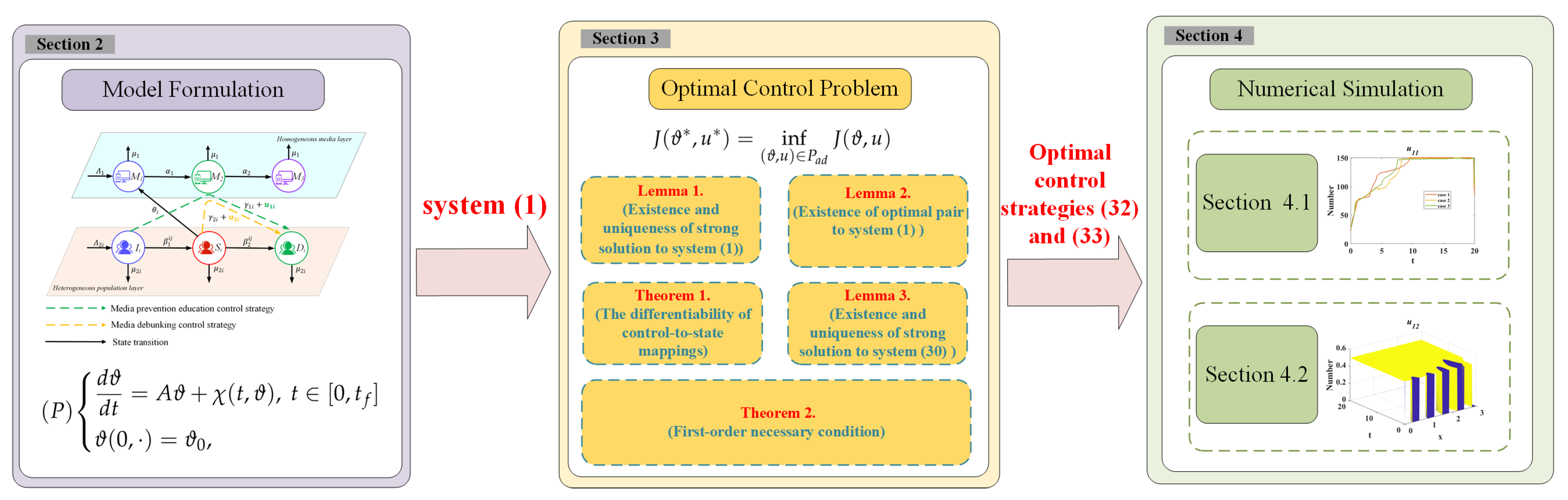
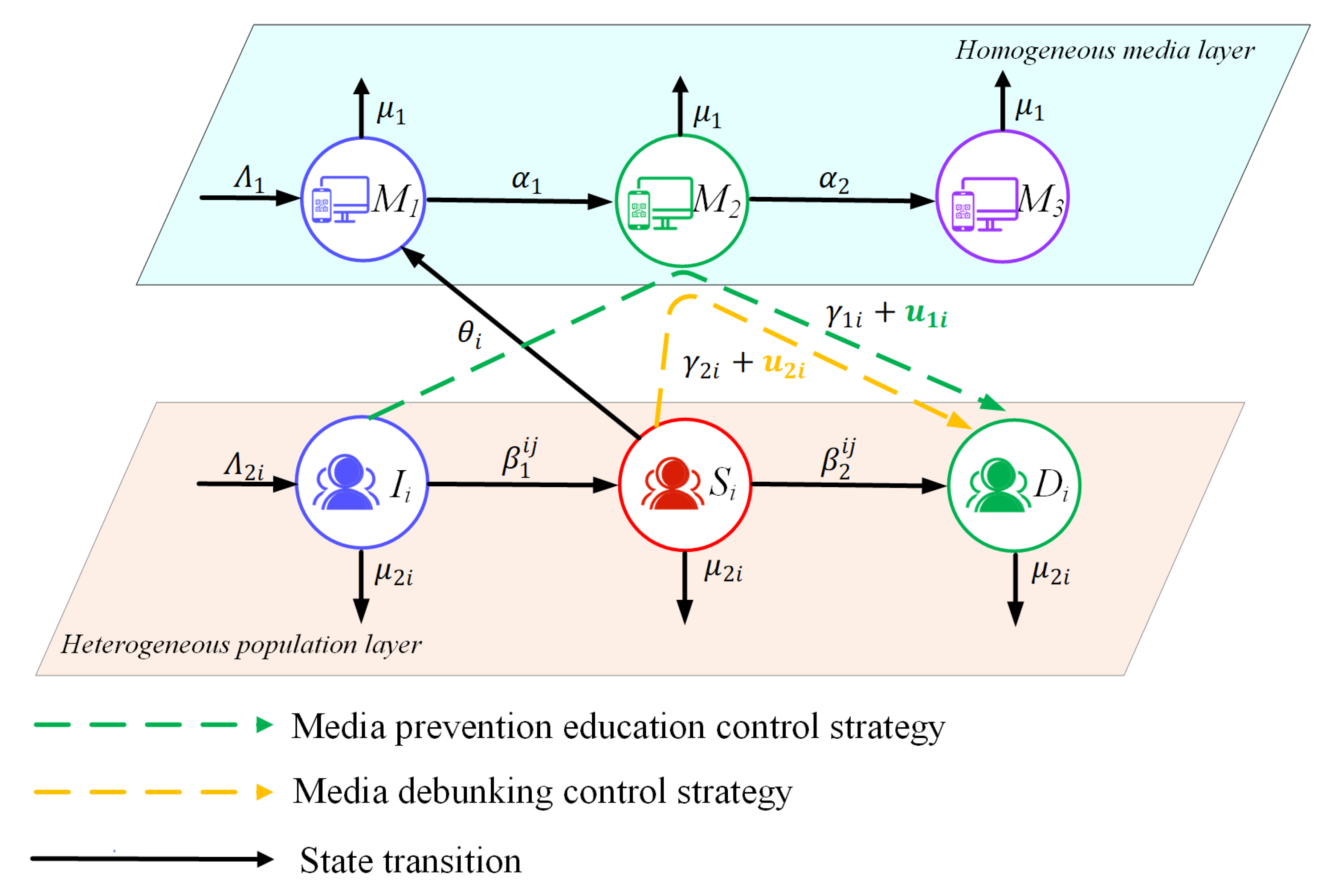
2. Model Formulation

2.1. Model Description

As illustrated in Figure 2, a hybrid dual-layer controlled model is established to capture the spatiotemporal propagation of rumors across regions under a multilingual environment and to enable indirect guidance via media platforms (e.g., YouTube, Twitter) for rumor mitigation. This model is composed of a homogeneous media layer and a heterogeneous population layer. In the homogeneous media layer, three platform states are distinguished: $M_1$ represents media platforms that do not participate in rumor dissemination and issue no statements; $M_2$ represents media platforms that actively publish debunking information; and $M_3$ represents media platforms that have deleted their debunking content but remain aware of the truth. The heterogeneous population layer partitions the global audience into m language-based subgroups. In each subgroup i, ignoramus ($I_i$) represents individuals who are unaware of both the rumor and the truth and thus prone to believing the rumor; spreaders ($S_i$) represent individuals who believe the rumor and actively propagate it; and debunkers ($D_i$) represent individuals who know the truth and actively disseminate corrections. Furthermore, two media-based spatiotemporal control measures are introduced:

• Media prevention education control strategy: Media platform $M_2$, for example, official outlets, issues authoritative information and pushes rumor-prevention notices on social networks, thereby increasing the probability that ignoramus $I_i$ encounters truthful information and converts it into active debunkers $D_i$. This is defined as the continuous control input $u_{1i}$.
• Media debunking control strategy: Media platform $M_2$ automatically flags misinformation warnings on spreader accounts and sends private messages containing evidential graphics and text, thereby increasing the probability that spreaders $S_i$ recognize the truthful information and convert it into active debunkers $D_i$. This is defined as the continuous control input $u_{2i}$.

Based on the foregoing discussion, the hybrid dual-layer controlled model, which is formulated on the basis of reaction–diffusion equations, may be expressed by the following system of equations.

$$\left\{\begin{array}{cc}\hfill {\partial }_t{I}_i=& D_{Pi}\Delta I_i+{\mathrm{\Lambda }}_{2i}-\sum _{j=1}^M{\beta }_1^{ij}{I}_i{S}_j-({\gamma }_{1i}+u_{1i})I_i{M}_2-{\mu }_{2i}{I}_i,in{\mathrm{\Omega }}_{t_f}\hfill \\ \hfill {\partial }_t{S}_i=& D_{Pi}\Delta S_k+\sum _{j=1}^M{\beta }_1^{ij}{I}_i{S}_i-({\gamma }_{2i}+u_{2i})S_i{M}_2-\sum _{j=1}^m{\beta }_2^{ij}{S}_i{D}_j-{\mu }_{2i}{S}_i,in{\mathrm{\Omega }}_{t_f}\hfill \\ \hfill {\partial }_t{D}_i=& D_{Pi}\Delta D_i+({\gamma }_{1i}+u_{1i})I_i{M}_2+({\gamma }_{2i}+u_{2i})S_i{M}_2+\sum _{j=1}^m{\beta }_2^{ij}{S}_i{D}_j-{\mu }_{2i}{D}_i,in{\mathrm{\Omega }}_{t_f}\hfill \\ \hfill {\partial }_t{M}_1=& D_M\Delta M_1+{\mathrm{\Lambda }}_1-\sum _{j=1}^m{\theta }_{1j}{M}_1{S}_i-{\alpha }_1{M}_1{M}_2-{\mu }_1{M}_1,in{\mathrm{\Omega }}_{t_f}\hfill \\ \hfill {\partial }_t{M}_2=& D_M\Delta M_2+\sum _{j=1}^m{\theta }_{1j}{M}_1{S}_i+{\alpha }_1{M}_1{M}_2-{\alpha }_2{M}_2-{\mu }_1{M}_2,in{\mathrm{\Omega }}_{t_f}\hfill \\ \hfill {\partial }_t{M}_3=& D_M\Delta M_3+{\alpha }_2{M}_2-{\mu }_1{M}_3,in{\mathrm{\Omega }}_{t_f}\hfill \\ \hfill {\displaystyle \frac{\partial I_i}{\partial t}}=& {\displaystyle \frac{\partial S_i}{\partial t}}={\displaystyle \frac{\partial D_i}{\partial t}}={\displaystyle \frac{\partial M_1}{\partial t}}={\displaystyle \frac{\partial M_2}{\partial t}}={\displaystyle \frac{\partial M_3}{\partial t}}=0,in{\Sigma }_{t_f}\hfill \\ \hfill I_i(0,·)& =0,S_i(0,·)=0,D_i(0,·)=0,M_1(0,·)=0,M_2(0,·)=0,M_3(0,·)=0.in\mathrm{\Omega }\hfill \end{array}\right.$$

(1)

where $\mathrm{\Omega }$ denotes a bounded domain with a sufficiently smooth boundary $\partial \mathrm{\Omega }$. Moreover, we define ${\mathrm{\Omega }}_{t_f}=\mathrm{\Omega }\times [0,t_f]$ and ${\Sigma }_{t_f}=\partial \mathrm{\Omega }\times [0,t_f]$. ${\partial }_n$ denotes the normal derivative on $\partial \mathrm{\Omega }$ in the direction of the outward unit normal vector n. In the reaction–diffusion system, the diffusion term represents the movement of individuals from regions of higher population density to regions of lower density. Accordingly, the one-dimensional spatial diffusion in each layer of the hybrid two-layer model is described by the Laplace operator $\Delta$, with diffusion intensities characterized by the coefficients $D_{pi}$ and $D_M$. The initial conditions $I_{i0},S_{i0},D_{i0},M_{10},M_{20}$ and $M_{30}$ are all taken to be positive constants. All other parameters are summarized in

Table 1. Parameter Descriptions.

Parameter	Description	Range
${\mathrm{\Lambda }}_1$	The rate of media-platform creation	$[0,1]$
${\mu }_1$	The probability of media-platform deactivation	$[0,1]$
${\alpha }_1$	The probability that the media platforms $M_1$ propagate	$[0,1]$
	debunking information issued by the media platforms $M_2$
${\alpha }_2$	The probability that the media platforms $M_2$ delete their	$[0,1]$
	debunking information
${\mathrm{\Lambda }}_{2i}$	The rate at which individuals in the i-th group become	$[0,1]$
	interested in rumor or truth
${\mu }_{2i}$	The probability that individuals in the i-th group lose	$[0,1]$
	interest in both rumor and truth
${\theta }_i$	The probability that $M_1$ becomes aware of the rumor via spreaders	$[0,1]$
	of the i-th group ($S_i$) and then issues debunking information
${\gamma }_{1i}$	The probability that the ignoramus $I_i$ from the i-th group accepts the	$[0,1]$
	truth upon encountering $M_2$’s debunking messages without intervention
${\gamma }_{2i}$	The probability that the spreaders $S_i$ from the i-th group accepts the	$[0,1]$
	truth upon encountering $M_2$’s debunking messages without intervention
${\beta }_1^{ij}$	The probability that the ignoramus $I_i$ believe the rumor	$[0,1]$
	by interacting with the spreaders $S_j$
${\beta }_2^{ij}$	The probability that the spreaders $S_i$ believe the truth by	$[0,1]$
	interacting with debunkers $D_j$

.

2.2. Preliminaries

In this paper, the workspace of the hybrid dual-layer model established in Section 2.1 is always the Hilbert space $H={\left[L^2\left(\mathrm{\Omega }\right)\right]}^{3m+3}$. Additionally, our model (1) is equivalent to

$$\left(P\right)\left\{\begin{array}{c}{\displaystyle \frac{d\vartheta }{dt}}=A\vartheta +\chi (t,\vartheta ),t\in [0,t_f],\hfill \\ \vartheta (0,·)={\vartheta }_0,\hfill \end{array}\right.$$

(2)

where $\vartheta ={(I_1,\dots ,I_m,S_1,\dots ,S_m,D_1,\dots ,D_m,M_1,M_2,M_3)}^T$ and $\chi (t,\vartheta )={({\chi }_{11}(t,\vartheta ),\dots ,{\chi }_{1m}(t,\vartheta ),\dots ,{\chi }_{31}(t,\vartheta ),\dots ,{\chi }_{3m}(t,\vartheta ),{\chi }_4(t,\vartheta ),{\chi }_5(t,\vartheta ),{\chi }_6(t,\vartheta ))}^T$ is defined as

$$\left\{\begin{array}{cc}\hfill {\chi }_{1i}=& {\mathrm{\Lambda }}_{2i}-\sum _{j=1}^M{\beta }_1^{ij}{I}_i{S}_j-({\gamma }_{1i}+u_{1i})I_i{M}_2-{\mu }_{2i}{I}_i,in{\mathrm{\Omega }}_{t_f}\hfill \\ \hfill {\chi }_{2i}=& \sum _{j=1}^M{\beta }_1^{ij}{I}_i{S}_i-({\gamma }_{2i}+u_{2i})S_i{M}_2-\sum _{j=1}^m{\beta }_2^{ij}{S}_i{D}_j-{\mu }_{2i}{S}_i,in{\mathrm{\Omega }}_{t_f}\hfill \\ \hfill {\chi }_{3i}=& ({\gamma }_{1i}+u_{1i})I_i{M}_2+({\gamma }_{2i}+u_{2i})S_i{M}_2+\sum _{j=1}^m{\beta }_2^{ij}{S}_i{D}_j-{\mu }_{2i}{D}_i,in{\mathrm{\Omega }}_{t_f}\hfill \\ \hfill {\chi }_4=& {\mathrm{\Lambda }}_1-\sum _{j=1}^m{\theta }_{1j}{M}_1{S}_i-{\alpha }_1{M}_1{M}_2-{\mu }_1{M}_1,in{\mathrm{\Omega }}_{t_f}\hfill \\ \hfill {\chi }_5=& \sum _{j=1}^m{\theta }_{1j}{M}_1{S}_i+{\alpha }_1{M}_1{M}_2-{\alpha }_2{M}_2-{\mu }_1{M}_2,in{\mathrm{\Omega }}_{t_f}\hfill \\ \hfill {\chi }_6=& {\alpha }_2{M}_2-{\mu }_1{M}_3.in{\mathrm{\Omega }}_{t_f}\hfill \end{array}\right.$$

(3)

where

$$\vartheta \in D\left(\chi \right)=\left\{\vartheta \in H:\chi (t,\vartheta )\in H,\forall t\in [0,t_f]\right\}$$

(4)

In addition, the linear operator A and the domain of A is defined is defined as follows

$$\begin{array}{cc}\hfill & A:D\left(A\right)\subseteq H\to H,\hfill \\ \hfill & A\vartheta =(D_{P1}\Delta I_1,\dots ,D_{Pm}\Delta I_m,D_{P1}\Delta S_1,\dots ,D_{Pm}\Delta S_m,D_{P1}\Delta D_1,\dots ,D_{Pm}\Delta D_m,D_M\Delta M_1,\hfill \\ \hfill & D_M\Delta M_2,D_M\Delta M_3{)}^T\in D\left(A\right),\forall \vartheta \in D\left(A\right)\hfill \end{array}$$

(5)

$$D\left(A\right)=\left\{\vartheta \in {\left[H^2\left(\mathrm{\Omega }\right)\right]}^{3m+3},{\displaystyle \frac{\partial {\vartheta }_{\tau }}{\partial n}}=0\mathrm{on}\partial \mathrm{\Omega },\tau =1,2,\dots ,3m+3\right\}$$

(6)

3. Optimal Control Problem

3.1. Preface

As a dynamic intervention strategy, optimal control techniques have been widely employed in the suppression of rumor propagation [3,24,25,26]. Over the finite time horizon $[0,t_f]$ and at the last time $t_f$, our primary goal is to minimize both the instantaneous and terminal populations of ignoramus $I_i$, spreaders $S_i$, and the debunking media platform $M_2$. Simultaneously, we must account for the implementation costs associated with the control measures. Since these objectives are inherently in tension, we introduce the following cost functional to balance the epidemiological impact of the controls against their economic expenditure:

$$\begin{array}{cc}\hfill J(\vartheta ,u)& ={\int }_0^{t_f}{\int }_{\mathrm{\Omega }}\left[\sum _{i=1}^m\left(A_{1i}{I}_i+A_{2i}{S}_i+B_{1i}{u}_{1i}+B_{2i}{u}_{2i}\right)+A_3{M}_2\right]dxdt\hfill \\ \hfill & +{\int }_{\mathrm{\Omega }}\left[\sum _{i=1}^m\left(C_{1i}{I}_i+C_{2i}{S}_i\right)+C_3{M}_2\right]dx\hfill \end{array}$$

(7)

where $A_{1i},A_{2i},A_3\in L^{\infty }\left({\mathrm{\Omega }}_{t_f}\right)$ and $A_{1i},A_{2i},A_3\in L^{\infty }\left(\mathrm{\Omega }\right)$ denote positive weights for state variables, $i=1,2,\dots ,m$; $B_{1i},B_{2i}\in L^{\infty }\left({\mathrm{\Omega }}_{t_f}\right)$ denote cost weights corresponding to media prevention education control strategy $u_{1i}$ and media debunking control strategy $u_{2i}$. Then, the admissible control set and the set of admissible pairs are defined as follows:

$$\begin{array}{cc}\hfill U_{ad}=& \{u={(u_{11},\dots ,u_{1m},u_{21},\dots ,u_{2m})}^T\in {\left[L^2\left({\mathrm{\Omega }}_{t_f}\right)\right]}^{2m}:0\le u_{1i},u_{2i}\le 0.5,\mathrm{a}.\mathrm{e}.\mathrm{in}{\mathrm{\Omega }}_{t_f},\hfill \\ & 1\le i\le m\}\hfill \end{array}$$

(8)

$$\begin{array}{cc}\hfill P_{ad}=& \{(\vartheta ,u):\vartheta ={(I_1,\dots ,I_m,S_1,\dots ,S_m,D_1,\dots ,D_m,M_1,M_2,M_3)}^T\mathrm{is}\mathrm{a}\mathrm{solution}\mathrm{of}\hfill \\ \hfill & \mathrm{system}\left(1\right)\mathrm{with}u\in U_{ad}\}\hfill \end{array}$$

(9)

Therefore, the optimal control problem can be formulated as follows: to find a solution that satisfies the hybrid dual layer controlled system (1). $({\vartheta }^{*},u^{*})\in P_{ad}$ in order to minimize the cost functional (7).

$$J({\vartheta }^{*},u^{*})=\underset{(\vartheta ,u)\in P_{ad}}{inf}J(\vartheta ,u)$$

(10)

Moreover, according to [27,28], we have the following result.

Lemma 1

(Existence and uniqueness of strong solution to system (1)). Let Ω be a bounded domain in ${\mathbb{R}}^n$, $n=1,2,3$, with smooth enough boundary $\partial \mathrm{\Omega }$. For any $u\in U_{ad}$, system (1) admits a unique strong positive solution $\vartheta \in {[W^{1,2}(0,t_f;L^2\left(\mathrm{\Omega }\right))\cap L^2(0,t_f;H^2\left(\mathrm{\Omega }\right))\cap L^{\infty }(0,t_f;H^1\left(\mathrm{\Omega }\right))\cap L^{\infty }\left({\mathrm{\Omega }}_{t_f}\right)]}^{3m+3}$. Additionally, independent of ϑ and u, there is a non-negative constant ϖ, such that

$$\begin{array}{cc}\hfill & {∥{\displaystyle \frac{\partial I_i}{\partial t}}∥}_{L^2\left({\mathrm{\Omega }}_{t_f}\right)}+{∥I_i∥}_{L^2(0,t_f;H^2\left(\mathrm{\Omega }\right))}+{∥I_i∥}_{L^{\infty }(0,t_f;H^1\left(\mathrm{\Omega }\right))}+{∥I_i∥}_{L^{\infty }\left({\mathrm{\Omega }}_{t_f}\right)}\le \varpi ,\hfill \\ \hfill & {∥{\displaystyle \frac{\partial S_i}{\partial t}}∥}_{L^2\left({\mathrm{\Omega }}_{t_f}\right)}+{∥S_i∥}_{L^2(0,t_f;H^2\left(\mathrm{\Omega }\right))}+{∥S_i∥}_{L^{\infty }(0,t_f;H^1\left(\mathrm{\Omega }\right))}+{∥S_i∥}_{L^{\infty }\left({\mathrm{\Omega }}_{t_f}\right)}\le \varpi ,\hfill \\ \hfill & {∥{\displaystyle \frac{\partial D_i}{\partial t}}∥}_{L^2\left({\mathrm{\Omega }}_{t_f}\right)}+{∥D_i∥}_{L^2(0,t_f;H^2\left(\mathrm{\Omega }\right))}+{∥D_i∥}_{L^{\infty }(0,t_f;H^1\left(\mathrm{\Omega }\right))}+{∥D_i∥}_{L^{\infty }\left({\mathrm{\Omega }}_{t_f}\right)}\le \varpi ,\hfill \\ \hfill & {∥{\displaystyle \frac{\partial M_1}{\partial t}}∥}_{L^2\left({\mathrm{\Omega }}_{t_f}\right)}+{∥M_1∥}_{L^2(0,t_f;H^2\left(\mathrm{\Omega }\right))}+{∥M_1∥}_{L^{\infty }(0,t_f;H^1\left(\mathrm{\Omega }\right))}+{∥M_1∥}_{L^{\infty }\left({\mathrm{\Omega }}_{t_f}\right)}\le \varpi ,\hfill \\ \hfill & {∥{\displaystyle \frac{\partial M_2}{\partial t}}∥}_{L^2\left({\mathrm{\Omega }}_{t_f}\right)}+{∥M_2∥}_{L^2(0,t_f;H^2\left(\mathrm{\Omega }\right))}+{∥M_2∥}_{L^{\infty }(0,t_f;H^1\left(\mathrm{\Omega }\right))}+{∥M_2∥}_{L^{\infty }\left({\mathrm{\Omega }}_{t_f}\right)}\le \varpi ,\hfill \\ \hfill & {∥{\displaystyle \frac{\partial M_3}{\partial t}}∥}_{L^2\left({\mathrm{\Omega }}_{t_f}\right)}+{∥M_3∥}_{L^2(0,t_f;H^2\left(\mathrm{\Omega }\right))}+{∥M_3∥}_{L^{\infty }(0,t_f;H^1\left(\mathrm{\Omega }\right))}+{∥M_3∥}_{L^{\infty }\left({\mathrm{\Omega }}_{t_f}\right)}\le \varpi .\hfill \end{array}$$

(11)

Lemma 2

(Existence of optimal pair to system (1)). Under the conditions of Lemma 1, the optimization problem (10) admits at least an optimal solution

$$({\vartheta }^{*},u^{*})\in P_{ad}.$$

(12)

Remark 1.

Since the relevant methods are well documented in [6,29,30], the proofs of Lemmas 1 and 2 are omitted here.

3.2. Necessary Optimality Conditions

In this section, we focus on establishing the first-order necessary conditions for the optimal control problem. Following [30,31], a mapping is introduced.

$$\begin{array}{cc}\hfill & M:U_{ad}\subset {\left[L^2\left({\mathrm{\Omega }}_{t_f}\right)\right]}^{2m}\to \mathrm{\Phi }\subset {\left[L^2\left({\mathrm{\Omega }}_{t_f}\right)\right]}^{3m+3},\mathrm{defined}\mathrm{by}{U}_{ad}\left(u\right):=\vartheta \left(u\right)=(I_1\left(u\right),\dots ,\hfill \\ & I_m\left(u\right),S_1\left(u\right),\dots ,S_m\left(u\right),D_1\left(u\right),\dots ,D_m\left(u\right),M_1\left(u\right),M_2\left(u\right),M_3{\left(u\right))}^T.\hfill \end{array}$$

where $\mathrm{\Phi }={[W^{1,2}(0,t_f;L^2\left(\mathrm{\Omega }\right))\cap L^2(0,t_f;H^2\left(\mathrm{\Omega }\right))\cap L^{\infty }(0,t_f;H^1\left(\mathrm{\Omega }\right))\cap L^{\infty }\left({\mathrm{\Omega }}_{t_f}\right)]}^{3m+3}$. $\vartheta \left(u\right)={(I_1\left(u\right),\dots ,I_m\left(u\right),S_1\left(u\right),\dots ,S_m\left(u\right),D_1\left(u\right),\dots ,D_m\left(u\right),M_1\left(u\right),M_2\left(u\right),M_3\left(u\right))}^T$ is a solution of system (1) corresponding to $u\in U_{ad}$. According to Lemma 1, the mapping M is well defined. Let ${\vartheta }^{\epsilon }={(I_1^{\epsilon },\dots ,I_m^{\epsilon },S_1^{\epsilon },\dots ,S_m^{\epsilon },D_1^{\epsilon },\dots ,D_m^{\epsilon },M_1^{\epsilon },M_2^{\epsilon },M_3^{\epsilon })}^T$ and ${\vartheta }^{*}={(I_1^{*},\dots ,I_m^{*},S_1^{*},\dots ,S_m^{*},D_1^{*},\dots ,D_m^{*},M_1^{*},M_2^{*},M_3^{*})}^T$ be the solutions of the system (1) corresponding to $u^{\epsilon }={(u_{11}^{\epsilon },\dots ,u_{1m}^{\epsilon },u_{21}^{\epsilon },\dots ,u_{2m}^{\epsilon })}^T\mathrm{and}{u}^{*}={(u_{11}^{*},\dots ,u_{1m}^{*},u_{21}^{*},\dots ,u_{2m}^{*})}^T$, respectively. Thus, the following results can be obtained.

Theorem 1

(The differentiability of control-to-state mappings). Under the condition of Lemma 1 and assuming $({\vartheta }^{*},u^{*})$ is an optimal pair acquired by Lemma 2. For any given $\tilde{u}\in L^2\left({\mathrm{\Omega }}_{t_f}\right)$ and $\epsilon >0$, take $u^{\epsilon }=u^{*}+\epsilon \tilde{u}$. Then the control-to-state mapping $M:u\to \vartheta \left(u\right)$ is Gâteaux differentiable at $u^{*}\in U_{ad}$. In particular, there exists a bounded linear operator $X:\tilde{u}\to z\left(\tilde{u}\right)$ such that

$$\underset{\epsilon \to 0}{lim}{∥{\displaystyle \frac{M\left(u^{\epsilon }\right)-M\left(u^{*}\right)}{\epsilon }}-z\left(\tilde{u}\right)∥}_H=0,\forall \tilde{u}\in {\left[L^2\left({\mathrm{\Omega }}_{t_f}\right)\right]}^{2m},$$

where $z\left(\tilde{u}\right)={({(z_{11}\left(\tilde{u}\right),\dots ,z_{1m}\left(\tilde{u}\right))}^T,\dots ,{(z_{31}\left(\tilde{u}\right),\dots ,z_{3m}\left(\tilde{u}\right))}^T,z_4\left(\tilde{u}\right),z_5\left(\tilde{u}\right),z_6\left(\tilde{u}\right))}^T$ is the solution of the following linearized system. The linear operator X is implicitly defined by system (13).

$$\left\{\begin{array}{cc}\hfill {\displaystyle \frac{\partial Z_{1i}}{\partial t}}=& D_{Pi}\Delta Z_{1i}+(-\sum _{j=1}^m{\beta }_1^{ij}{S}_j^{*}-{\gamma }_{1i}{M}_2^{*}-u_{1i}^{*}{M}_2^{*}-{\mu }_{2i})Z_{1i}-\sum _{j=1}^m{\beta }_1^{ij}{I}_i^{*}{Z}_{2j}+(-{\gamma }_{1i}{I}_i^{*}\hfill \\ \hfill & -u_{1i}^{*}{I}_i^{*})Z_5-\widetilde{u_{1i}}{I}_i^{*}{M}_2^{*},in{\mathrm{\Omega }}_{t_f}\hfill \\ \hfill {\displaystyle \frac{\partial Z_{2i}}{\partial t}}=& D_{Pi}\Delta Z_{2i}+\sum _{j=1}^m{\beta }_1^{ij}{S}_j^{*}{Z}_{1i}+\sum _{j=1}^m{\beta }_1^{ij}{I}_i^{*}{Z}_{2j}+(-{\gamma }_{2i}{M}_2^{*}-u_{2i}^{*}{M}_2^{*}-\sum _{j=1}^m{\beta }_2^{ij}{D}_j^{*}-{\mu }_{2i})Z_{2i}\hfill \\ \hfill & -\sum _{j=1}^m{\beta }_2^{ij}{S}_i^{*}{Z}_{3j}+(-{\gamma }_{2i}{S}_i^{*}-u_{2i}^{*}{S}_i^{*})Z_5-\widetilde{u_{2i}}{S}_i^{*}{M}_2^{*},in{\mathrm{\Omega }}_{t_f}\hfill \\ \hfill {\displaystyle \frac{\partial Z_{3i}}{\partial t}}=& D_{Pi}\Delta Z_{3i}+({\gamma }_{1i}{M}_2^{*}+u_{1i}^{*}{M}_2^{*})Z_{1i}+({\gamma }_{2i}{M}_2^{*}+u_{2i}^{*}{M}_2^{*}+\sum _{j=1}^m{\beta }_2^{ij}{D}_j)Z_{2i}+\sum _{j=1}^m{\beta }_2^{ij}{S}_i^{*}{Z}_{3j}\hfill \\ \hfill & -{\mu }_{2i}{Z}_{3i}+({\gamma }_{1i}{I}_i^{*}+u_{1i}^{*}{I}_i^{*}+{\gamma }_{2i}{S}_i^{*}+u_{2i}^{*}{S}_i^{*})Z_5+\widetilde{u_{1i}}{I}_i^{*}{M}_2^{*}+\widetilde{u_{2i}}{S}_i^{*}{M}_2^{*},in{\mathrm{\Omega }}_{t_f}\hfill \\ \hfill {\displaystyle \frac{\partial Z_4}{\partial t}}=& D_M\Delta Z_4-\sum _{j=1}^m{\theta }_j{M}_1^{*}{Z}_{2j}+(-\sum _{j=1}^m{S}_j^{*}{\theta }_j-{\alpha }_1{M}_2^{*}-{\mu }_1)Z_4-{\alpha }_1{M}_1^{*}{Z}_5,in{\mathrm{\Omega }}_{t_f}\hfill \\ \hfill {\displaystyle \frac{\partial Z_5}{\partial t}}=& D_M\Delta Z_5+\sum _{j=1}^m{\theta }_j{M}_1^{*}{Z}_{2j}+(\sum _{j=1}^m{S}_j^{*}{\theta }_j+{\alpha }_1{M}_2^{*})Z_4+({\alpha }_1{M}_1^{*}-{\alpha }_2-{\mu }_1)Z_5,in{\mathrm{\Omega }}_{t_f}\hfill \\ \hfill {\displaystyle \frac{\partial Z_6}{\partial t}}=& D_M\Delta Z_6+{\alpha }_2{Z}_5-{\mu }_1{Z}_6,in{\mathrm{\Omega }}_{t_f}\hfill \\ \hfill {\displaystyle \frac{\partial Z_{1i}}{\partial t}}=& {\displaystyle \frac{\partial Z_{2i}}{\partial t}}={\displaystyle \frac{\partial Z_{3i}}{\partial t}}={\displaystyle \frac{\partial Z_4}{\partial t}}={\displaystyle \frac{\partial Z_5}{\partial t}}={\displaystyle \frac{\partial Z_6}{\partial t}}=0,in{\Sigma }_{t_f}\hfill \\ \hfill Z_{1i}(0,·)& =0,Z_{2i}(0,·)=0,Z_{3i}(0,·)=0,Z_4(0,·)=0,Z_5(0,·)=0,Z_6(0,·)=0.in\mathrm{\Omega }\hfill \end{array}\right.$$

(13)

Proof. 

Denote

$$z^{\epsilon }:={\displaystyle \frac{M\left(u^{\epsilon }\right)-M\left(u^{*}\right)}{\epsilon }}={({(z_{11}^{\epsilon },\dots ,z_{1m}^{\epsilon })}^T,\dots ,{(z_{31}^{\epsilon },\dots ,z_{3m}^{\epsilon })}^T,z_4^{\epsilon },z_5^{\epsilon },z_6^{\epsilon })}^T.$$

(14)

Remarkably, the following assumption is introduced for convenience.

$$Z_{2i}={\displaystyle \frac{S_i^{\epsilon }-S_i^{*}}{\epsilon }}={\displaystyle \frac{S_j^{\epsilon }-S_i^{*}}{\epsilon }}=Z_{2j},Z_{3i}={\displaystyle \frac{D_i^{\epsilon }-D_i^{*}}{\epsilon }}={\displaystyle \frac{D_j^{\epsilon }-D_i^{*}}{\epsilon }}=Z_{3j}.$$

Then, X is a linear bounded operator from ${\left[L^2\left({\mathrm{\Omega }}_{t_f}\right)\right]}^{2m}$ to ${\left[L^2\left({\mathrm{\Omega }}_{t_f}\right)\right]}^{3m+3}$ will be demonstrated that with satisfying

$$\underset{\epsilon \to 0}{lim}{\parallel z^{\epsilon }-z\parallel }_H=0,\forall \tilde{u}\in {\left[L^2\left({\mathrm{\Omega }}_{t_f}\right)\right]}^{2m}.$$

(15)

Additionally, one can show that $z^{\epsilon }$ satisfies the following system

$$\left\{\begin{array}{cc}\hfill {\displaystyle \frac{\partial Z_{1i}^{\epsilon }}{\partial t}}=& D_{Pi}\Delta Z_{1i}^{\epsilon }+(-\sum _{j=1}^m{\beta }_1^{ij}{S}_j^{\epsilon }-{\gamma }_{1i}{M}_2^{\epsilon }-u_{1i}^{*}{M}_2^{\epsilon }-{\mu }_{2i})Z_{1i}^{\epsilon }-\sum _{j=1}^m{\beta }_1^{ij}{I}_i^{*}{Z}_{2j}^{\epsilon }+(-{\gamma }_{1i}{I}_i^{*}\hfill \\ \hfill & -u_{1i}^{*}{I}_i^{*})Z_5^{\epsilon }-\widetilde{u_{1i}}{I}_i^{\epsilon }{M}_2^{\epsilon },in{\mathrm{\Omega }}_{t_f}\hfill \\ \hfill {\displaystyle \frac{\partial Z_{2i}^{\epsilon }}{\partial t}}=& D_{Pi}\Delta Z_{2i}^{\epsilon }+\sum _{j=1}^m{\beta }_1^{ij}{S}_j^{\epsilon }{Z}_{1i}^{\epsilon }+\sum _{j=1}^m{\beta }_1^{ij}{I}_i^{*}{Z}_{2j}^{\epsilon }+(-{\gamma }_{2i}{M}_2^{\epsilon }-u_{2i}^{*}{M}_2^{\epsilon }-\sum _{j=1}^m{\beta }_2^{ij}{D}_j^{\epsilon }-{\mu }_{2i})Z_{2i}^{\epsilon }\hfill \\ \hfill & -\sum _{j=1}^m{\beta }_2^{ij}{S}_i^{*}{Z}_{3j}^{\epsilon }+(-{\gamma }_{2i}{S}_i^{*}-u_{2i}^{*}{S}_i^{*})Z_5^{\epsilon }-\widetilde{u_{2i}}{S}_i^{\epsilon }{M}_2^{\epsilon },in{\mathrm{\Omega }}_{t_f}\hfill \\ \hfill {\displaystyle \frac{\partial Z_{3i}^{\epsilon }}{\partial t}}=& D_{Pi}\Delta Z_{3i}^{\epsilon }+({\gamma }_{1i}{M}_2^{\epsilon }+u_{1i}^{*}{M}_2^{\epsilon })Z_{1i}^{\epsilon }+({\gamma }_{2i}{M}_2^{\epsilon }+u_{2i}^{*}{M}_2^{\epsilon }+\sum _{j=1}^m{\beta }_2^{ij}{D}_j^{\epsilon })Z_{2i}^{\epsilon }+\sum _{j=1}^m{\beta }_2^{ij}{S}_i^{*}{Z}_{3j}^{\epsilon }\hfill \\ \hfill & -{\mu }_{2i}{Z}_{3i}^{\epsilon }+({\gamma }_{1i}{I}_i^{*}+u_{1i}^{*}{I}_i^{*}+{\gamma }_{2i}{S}_i^{*}+u_{2i}^{*}{S}_i^{*})Z_5^{\epsilon }+\widetilde{u_{1i}}{I}_i^{\epsilon }{M}_2^{\epsilon }+\widetilde{u_{2i}}{S}_i^{\epsilon }{M}_2^{\epsilon },in{\mathrm{\Omega }}_{t_f}\hfill \\ \hfill {\displaystyle \frac{\partial Z_4^{\epsilon }}{\partial t}}=& D_M\Delta Z_4^{\epsilon }-\sum _{j=1}^m{\theta }_j{M}_1^{*}{Z}_{2j}^{\epsilon }+(-\sum _{j=1}^m{S}_j^{\epsilon }{\theta }_j-{\alpha }_1{M}_2^{\epsilon }-{\mu }_1)Z_4^{\epsilon }-{\alpha }_1{M}_1^{*}{Z}_5^{\epsilon },in{\mathrm{\Omega }}_{t_f}\hfill \\ \hfill {\displaystyle \frac{\partial Z_5^{\epsilon }}{\partial t}}=& D_M\Delta Z_5^{\epsilon }+\sum _{j=1}^m{\theta }_j{M}_1^{*}{Z}_{2j}^{\epsilon }+(\sum _{j=1}^m{S}_j^{\epsilon }{\theta }_j+{\alpha }_1{M}_2^{\epsilon })Z_4^{\epsilon }+({\alpha }_1{M}_1^{*}-{\alpha }_2-{\mu }_1)Z_5^{\epsilon },in{\mathrm{\Omega }}_{t_f}\hfill \\ \hfill {\displaystyle \frac{\partial Z_6^{\epsilon }}{\partial t}}=& D_M\Delta Z_6^{\epsilon }+{\alpha }_2{Z}_5^{\epsilon }-{\mu }_1{Z}_6^{\epsilon },in{\mathrm{\Omega }}_{t_f}\hfill \\ \hfill {\displaystyle \frac{\partial Z_{1i}^{\epsilon }}{\partial t}}=& {\displaystyle \frac{\partial Z_{2i}^{\epsilon }}{\partial t}}={\displaystyle \frac{\partial Z_{3i}^{\epsilon }}{\partial t}}={\displaystyle \frac{\partial Z_4^{\epsilon }}{\partial t}}={\displaystyle \frac{\partial Z_5^{\epsilon }}{\partial t}}={\displaystyle \frac{\partial Z_6^{\epsilon }}{\partial t}}=0,in{\Sigma }_{t_f}\hfill \\ \hfill Z_{1i}^{\epsilon }(0,·)& =0,Z_{2i}^{\epsilon }(0,·)=0,Z_{3i}^{\epsilon }(0,·)=0,Z_4^{\epsilon }(0,·)=0,Z_5^{\epsilon }(0,·)=0,Z_6^{\epsilon }(0,·)=0.in\mathrm{\Omega }\hfill \end{array}\right.$$

(16)

Set

$${\mathrm{\Theta }}^{\epsilon }\left(t\right)=\left(\begin{array}{cccccc}{\mathrm{\Theta }}_{1-1i}^{\epsilon }& {\mathrm{\Theta }}_{1-2i}^{\epsilon }& \mathbf{0}& \mathbf{0}& {\mathrm{\Theta }}_{1-5i}^{\epsilon }& \mathbf{0}\\ {\mathrm{\Theta }}_{2-1i}^{\epsilon }& {\mathrm{\Theta }}_{2-2i}^{\epsilon }& {\mathrm{\Theta }}_{2-3i}^{\epsilon }& \mathbf{0}& {\mathrm{\Theta }}_{2-5i}^{\epsilon }& \mathbf{0}\\ {\mathrm{\Theta }}_{3-1i}^{\epsilon }& {\mathrm{\Theta }}_{3-2i}^{\epsilon }& {\mathrm{\Theta }}_{3-3i}^{\epsilon }& \mathbf{0}& {\mathrm{\Theta }}_{3-5i}^{\epsilon }& \mathbf{0}\\ \mathbf{0}& {\mathrm{\Theta }}_{4-2i}^{\epsilon }& \mathbf{0}& {\mathrm{\Theta }}_{4-4}^{\epsilon }& {\mathrm{\Theta }}_{4-5}^{\epsilon }& \mathbf{0}\\ \mathbf{0}& {\mathrm{\Theta }}_{5-2i}^{\epsilon }& \mathbf{0}& {\mathrm{\Theta }}_{5-4}^{\epsilon }& {\mathrm{\Theta }}_{5-5}^{\epsilon }& \mathbf{0}\\ \mathbf{0}& \mathbf{0}& \mathbf{0}& \mathbf{0}& {\mathrm{\Theta }}_{6-5}^{\epsilon }& {\mathrm{\Theta }}_{6-6}^{\epsilon }\end{array}\right)$$

(17)

where

$$\begin{array}{cc}\hfill & {\mathrm{\Theta }}_{1-1i}^{\epsilon }=-\sum _{j=1}^m{\beta }_1^{ij}{S}_j^{\epsilon }-{\gamma }_{1i}{M}_2^{\epsilon }-u_{1i}^{*}{M}_2^{\epsilon }-{\mu }_{2i},{\mathrm{\Theta }}_{1-2i}^{\epsilon }=-\sum _{j=1}^m{\beta }_1^{ij}{I}_i^{*},{\mathrm{\Theta }}_{1-5i}^{\epsilon }=-{\gamma }_{1i}{I}_i^{*}-u_{1i}^{*}{I}_i^{*},\hfill \\ \hfill & {\mathrm{\Theta }}_{2-1i}^{\epsilon }=\sum _{j=1}^m{\beta }_1^{ij}{S}_j^{\epsilon },{\mathrm{\Theta }}_{2-2i}^{\epsilon }=\sum _{j=1}^m{\beta }_1^{ij}{I}_i^{*}-{\gamma }_{2i}{M}_2^{\epsilon }-u_{2i}^{*}{M}_2^{\epsilon }-\sum _{j=1}^m{\beta }_2^{ij}{D}_j^{\epsilon }-{\mu }_{2i},{\mathrm{\Theta }}_{2-3i}^{\epsilon }=-\sum _{j=1}^m{\beta }_2^{ij}{S}_i^{*},\hfill \\ \hfill & {\mathrm{\Theta }}_{2-5i}^{\epsilon }=-{\gamma }_{2i}{S}_i^{*}-u_{2i}^{*}{S}_i^{*},{\mathrm{\Theta }}_{3-1i}^{\epsilon }={\gamma }_{1i}{M}_2^{\epsilon }+u_{1i}^{*}{M}_2^{\epsilon },{\mathrm{\Theta }}_{3-2i}^{\epsilon }={\gamma }_{2i}{M}_2^{\epsilon }+u_{2i}^{*}{M}_2^{\epsilon }+\sum _{j=1}^m{\beta }_2^{ij}{D}_j^{\epsilon },\hfill \\ \hfill & {\mathrm{\Theta }}_{3-3i}^{\epsilon }=\sum _{j=1}^m{\beta }_2^{ij}{S}_i^{*}-{\mu }_{2i},{\mathrm{\Theta }}_{3-5i}^{\epsilon }={\gamma }_{1i}{I}_i^{*}+u_{1i}^{*}{I}_i^{*}+{\gamma }_{2i}{S}_i^{*}+u_{2i}^{*}{S}_i^{*},{\mathrm{\Theta }}_{4-2i}^{\epsilon }=-{\theta }_i{M}_1^{*},\hfill \\ \hfill & {\mathrm{\Theta }}_{4-4}^{\epsilon }=-\sum _{j=1}^m{S}_j^{\epsilon }{\theta }_j-{\alpha }_1{M}_2^{\epsilon }-{\mu }_1,{\mathrm{\Theta }}_{4-5}^{\epsilon }=-{\alpha }_1{M}_1^{*},{\mathrm{\Theta }}_{5-2i}^{\epsilon }={\theta }_i{M}_1^{*},\hfill \\ \hfill & {\mathrm{\Theta }}_{5-4}^{\epsilon }=\sum _{j=1}^m{S}_j^{\epsilon }{\theta }_j+{\alpha }_1{M}_2^{\epsilon },{\mathrm{\Theta }}_{5-5}^{\epsilon }={\alpha }_1{M}_1^{*}-{\alpha }_2-{\mu }_1,{\mathrm{\Theta }}_{6-5}^{\epsilon }={\alpha }_2,{\mathrm{\Theta }}_{6-6}^{\epsilon }=-{\mu }_1,\hfill \end{array}$$

$$\begin{array}{cc}\hfill & {\mathrm{\Theta }}_{1-\delta }^{\epsilon }=({\mathrm{\Theta }}_{1-{\delta }_1}^{\epsilon },\dots ,{\mathrm{\Theta }}_{1-{\delta }_m}^{\epsilon }),\delta =1,2,5,\hfill \\ \hfill & {\mathrm{\Theta }}_{2-\delta }^{\epsilon }=({\mathrm{\Theta }}_{2-{\delta }_1}^{\epsilon },\dots ,{\mathrm{\Theta }}_{2-{\delta }_m}^{\epsilon }),\delta =1,2,3,5,\hfill \\ \hfill & {\mathrm{\Theta }}_{3-\delta }^{\epsilon }=({\mathrm{\Theta }}_{3-{\delta }_1}^{\epsilon },\dots ,{\mathrm{\Theta }}_{3-{\delta }_m}^{\epsilon }),\delta =1,2,3,5,\hfill \\ \hfill & {\mathrm{\Theta }}_{4-\delta }^{\epsilon }=({\mathrm{\Theta }}_{4-{\delta }_1}^{\epsilon },\dots ,{\mathrm{\Theta }}_{4-{\delta }_m}^{\epsilon }),\delta =2,\hfill \\ \hfill & {\mathrm{\Theta }}_{5-\delta }^{\epsilon }=({\mathrm{\Theta }}_{5-{\delta }_1}^{\epsilon },\dots ,{\mathrm{\Theta }}_{5-{\delta }_m}^{\epsilon }),\delta =2,\hfill \end{array}$$

(18)

and

$$\begin{array}{c}\hfill \psi \left(t\right)={({\psi }_1,{\psi }_2,{\psi }_3,{\psi }_4,{\psi }_5,{\psi }_6)}^T,\end{array}$$

with

$$\begin{array}{cc}\hfill & {\psi }_{1i}=-\widetilde{u_{1i}}{I}_i^{\epsilon }{M}_2^{\epsilon },{\psi }_{2i}=-\widetilde{u_{2i}}{S}_i^{\epsilon }{M}_2^{\epsilon },{\psi }_{3i}=\widetilde{u_{1i}}{I}_i^{\epsilon }{M}_2^{\epsilon }+\widetilde{u_{2i}}{S}_i^{\epsilon }{M}_2^{\epsilon },{\psi }_4=-{\alpha }_1{M}_1^{*}{Z}_5^{\epsilon },\hfill \\ \hfill & {\psi }_1={({\psi }_{11},\dots ,{\psi }_{1m})}^T,{\psi }_2={({\psi }_{21},\dots ,{\psi }_{2m})}^T,{\psi }_3={({\psi }_{31},\dots ,{\psi }_{3m})}^T.\hfill \end{array}$$

Thus, system (16) can be rewritten as follows

$$\left\{\begin{array}{c}{\displaystyle \frac{\partial z^{\epsilon }}{\partial t}}=\mathcal{A}{z}^{\epsilon }+{\mathrm{\Theta }}^{\epsilon }\left(t\right)z^{\epsilon }+\psi \left(t\right),t\in (0,T),\hfill \\ z^{\epsilon }(0,·)=0,\hfill \end{array}\right.$$

(19)

where $\mathcal{A}$ is defined in (5) and (6). Hence, system (19) has a unique strong solution that can be derived by the semigroup arguments.

$$z^{\epsilon }\left(t\right)={\int }_0^{t}S(t-s){\mathrm{\Theta }}^{\epsilon }\left(s\right)z^{\epsilon }\left(s\right)ds+{\int }_0^{t}S(t-s)\psi \left(s\right)ds,\forall t\in [0,t_f],$$

(20)

where $\left\{S\right(t),t\ge 0\}$ represents the semigroup generated by $\mathcal{A}$. Furthermore, due to all elements of matrix ${\phi }^{\epsilon }\left(t\right)$ and $\psi \left(t\right)$ are uniformly bounded. By the $L^p$ theory for linear parabolic equations, it follows that there exists a constant $C_1>0$, independent of $\epsilon$, such that

$$\parallel z^{\epsilon }{\left(t\right)\parallel }_H\le C_1{\int }_0^t{\parallel \psi \left(t\right)\parallel }_H\le C_1,\forall t\in [0,t_f].$$

(21)

Invoking the definition of $z^{\epsilon }$, it readily follows that, as $\epsilon \to 0$,

$$I_{1i}^{\epsilon }\to I_{1i},S_{2i}^{\epsilon }\to S_{2i},D_{3i}^{\epsilon }\to D_{3i},M_1^{\epsilon }\to M_1,M_2^{\epsilon }\to M_2,M_3^{\epsilon }\to M_3\mathrm{in}{L}^2\left({\mathrm{\Omega }}_{t_f}\right),i=1,2,\dots ,m.$$

Similarly, system (13) can be reformulated as follows:

$$\left\{\begin{array}{c}{\displaystyle \frac{\partial z}{\partial t}}=\mathcal{A}z+\phi \left(t\right)z+\psi \left(t\right),t\in (0,T),\hfill \\ z(0,·)=0.\hfill \end{array}\right.$$

(22)

With

$$\mathrm{\Theta }\left(t\right)=\left(\begin{array}{cccccc}{\mathrm{\Theta }}_{1-1i}& {\mathrm{\Theta }}_{1-2i}& \mathbf{0}& \mathbf{0}& {\mathrm{\Theta }}_{1-5i}& \mathbf{0}\\ {\mathrm{\Theta }}_{2-1i}& {\mathrm{\Theta }}_{2-2i}& {\mathrm{\Theta }}_{2-3i}& \mathbf{0}& {\mathrm{\Theta }}_{2-5i}& \mathbf{0}\\ {\mathrm{\Theta }}_{3-1i}& {\mathrm{\Theta }}_{3-2i}& {\mathrm{\Theta }}_{3-3i}& \mathbf{0}& {\mathrm{\Theta }}_{3-5i}& \mathbf{0}\\ \mathbf{0}& {\mathrm{\Theta }}_{4-2i}& \mathbf{0}& {\mathrm{\Theta }}_{4-4}& {\mathrm{\Theta }}_{4-5}& \mathbf{0}\\ \mathbf{0}& {\mathrm{\Theta }}_{5-2i}& \mathbf{0}& {\mathrm{\Theta }}_{5-4}& {\mathrm{\Theta }}_{5-5}& \mathbf{0}\\ \mathbf{0}& \mathbf{0}& \mathbf{0}& \mathbf{0}& {\mathrm{\Theta }}_{6-5}& {\mathrm{\Theta }}_{6-6}\end{array}\right)$$

(23)

and

$$\begin{array}{cc}\hfill & {\mathrm{\Theta }}_{1-1i}=-\sum _{j=1}^m{\beta }_1^{ij}{S}_j^{*}-{\gamma }_{1i}{M}_2^{*}-u_{1i}^{*}{M}_2^{*}-{\mu }_{2i},{\mathrm{\Theta }}_{1-2i}=-\sum _{j=1}^m{\beta }_1^{ij}{I}_i^{*},{\mathrm{\Theta }}_{1-5i}=-{\gamma }_{1i}{I}_i^{*}-u_{1i}^{*}{I}_i^{*},\hfill \\ \hfill & {\mathrm{\Theta }}_{2-1i}=\sum _{j=1}^m{\beta }_1^{ij}{S}_j^{*},{\mathrm{\Theta }}_{2-2i}=\sum _{j=1}^m{\beta }_1^{ij}{I}_i^{*}-{\gamma }_{2i}{M}_2^{*}-u_{2i}^{*}{M}_2^{*}-\sum _{j=1}^m{\beta }_2^{ij}{D}_j^{*}-{\mu }_{2i},{\mathrm{\Theta }}_{2-3i}=-\sum _{j=1}^m{\beta }_2^{ij}{S}_i^{*},\hfill \\ \hfill & {\mathrm{\Theta }}_{2-5i}=-{\gamma }_{2i}{S}_i^{*}-u_{2i}^{*}{S}_i^{*},{\mathrm{\Theta }}_{3-1i}={\gamma }_{1i}{M}_2^{*}+u_{1i}^{*}{M}_2^{*},{\mathrm{\Theta }}_{3-2i}={\gamma }_{2i}{M}_2^{*}+u_{2i}^{*}{M}_2^{*}+\sum _{j=1}^m{\beta }_2^{ij}{D}_j,\hfill \\ \hfill & {\mathrm{\Theta }}_{3-3i}=\sum _{j=1}^m{\beta }_2^{ij}{S}_i^{*}-{\mu }_{2i},{\mathrm{\Theta }}_{3-5i}={\gamma }_{1i}{I}_i^{*}+u_{1i}^{*}{I}_i^{*}+{\gamma }_{2i}{S}_i^{*}+u_{2i}^{*}{S}_i^{*},{\mathrm{\Theta }}_{4-2i}=-\sum _{j=1}^m{\theta }_j{M}_1^{*},\hfill \\ \hfill & {\mathrm{\Theta }}_{4-4}=-\sum _{j=1}^m{S}_j^{*}{\theta }_j-{\alpha }_1{M}_2^{*}-{\mu }_1,{\mathrm{\Theta }}_{4-5}=-{\alpha }_1{M}_1^{*},{\mathrm{\Theta }}_{5-2i}=\sum _{j=1}^m{\theta }_j{M}_1^{*},\hfill \\ \hfill & {\mathrm{\Theta }}_{5-4}=\sum _{j=1}^m{S}_j^{*}{\theta }_j+{\alpha }_1{M}_2^{*},{\mathrm{\Theta }}_{5-5}={\alpha }_1{M}_1^{*}-{\alpha }_2-{\mu }_1,{\mathrm{\Theta }}_{6-5}={\alpha }_2,{\mathrm{\Theta }}_{6-6}=-{\mu }_1,\hfill \\ \hfill & {\mathrm{\Theta }}_{1-\delta }=({\mathrm{\Theta }}_{1-{\delta }_1},\dots ,{\mathrm{\Theta }}_{1-{\delta }_m}),\delta =1,2,5,\hfill \\ \hfill & {\mathrm{\Theta }}_{2-\delta }=({\mathrm{\Theta }}_{2-{\delta }_1},\dots ,{\mathrm{\Theta }}_{2-{\delta }_m}),\delta =1,2,3,5,\hfill \\ \hfill & {\mathrm{\Theta }}_{3-\delta }=({\mathrm{\Theta }}_{3-{\delta }_1},\dots ,{\mathrm{\Theta }}_{3-{\delta }_m}),\delta =1,2,3,5,\hfill \\ \hfill & {\mathrm{\Theta }}_{4-\delta }=({\mathrm{\Theta }}_{4-{\delta }_1},\dots ,{\mathrm{\Theta }}_{4-{\delta }_m}),\delta =2,\hfill \\ \hfill & {\mathrm{\Theta }}_{5-\delta }=({\mathrm{\Theta }}_{5-{\delta }_1},\dots ,{\mathrm{\Theta }}_{5-{\delta }_m}),\delta =2.\hfill \end{array}$$

(24)

Following an argument analogous to that employed for system (19), we can likewise demonstrate that system (22) admits a unique strong solution.

$$z\left(t\right)={\int }_0^{t}S(t-s)\phi \left(s\right)z\left(s\right)ds+{\int }_0^{t}S(t-s)\psi \left(s\right)ds,\forall t\in [0,t_f].$$

(25)

By applying Equations (20) and (25), we obtain

$$\begin{array}{cc}\hfill z^{\epsilon }\left(t\right)-z\left(t\right)& ={\int }_0^{t}S(t-s)\left[{\phi }^{\epsilon }\left(s\right)z^{\epsilon }\left(s\right)-\phi \left(s\right)z\left(s\right)\right]ds\hfill \\ \hfill & ={\int }_0^{t}S(t-s)\left({\phi }^{\epsilon }\left(s\right)-\phi \left(s\right)\right)z^{\epsilon }\left(s\right)ds+{\int }_0^{t}S(t-s)\phi \left(s\right)\left(z^{\epsilon }\left(s\right)-z\left(s\right)\right)ds.\hfill \end{array}$$

(26)

Since the entries of both ${\phi }^{\epsilon }\left(t\right)$ and $\phi \left(t\right)$ are uniformly bounded, and each entry of ${\phi }^{\epsilon }\left(t\right)$ converges to the corresponding entry of $\phi \left(t\right)$ in $L^2\left({\mathrm{\Omega }}_{t_f}\right)$, it immediately follows that

$$\underset{\epsilon \to 0}{lim}{\parallel {\phi }^{\epsilon }\left(t\right)-\phi \left(t\right)\parallel }_{L^{\infty }({\mathrm{\Omega }}_{t_f})}=0.$$

(27)

Moreover, by applying Gronwall’s inequality, we acquire

$$\underset{\epsilon \to 0}{lim}{\parallel z^{\epsilon }\left(s\right)-z\left(s\right)\parallel }_H=0.$$

(28)

Furthermore, the linearized system (13) indicates that the operator X is linear. Its boundedness, in turn, is obtained directly from (22) by invoking the $L^p$ theory for linear parabolic equations.

$$\parallel z\left(\tilde{u}\right){\parallel }_H\le C_2{\parallel \tilde{u}\parallel }_{{\left[L^2\left({\mathrm{\Omega }}_T\right)\right]}^{2m}},$$

(29)

where $C_2$ is a non-negative constant independent of $\epsilon$. Hence, the control-to-state mapping M is Gâteaux differentiable at $u^{*}\in U_{ad}$. This completes the proof. □

In order to derive the first-order necessary conditions for system (1), following [32], the associated adjoint system is furthermore introduced.

$$\left\{\begin{array}{cc}\hfill {\lambda }_{1i}=& -D_{Pi}{\lambda }_{1i}+[\sum _{j=1}^m{\beta }_1^{ij}{S}_j^{*}+({\gamma }_{1i}+u_{1i}^{*})M_2^{*}+{\mu }_{2i}]{\lambda }_{1i}-\sum _{j=1}^m{S}_j^{*}{\lambda }_{2i}-({\gamma }_{1i}+u_{1i}^{*})M_2^{*}{\lambda }_{3i}\hfill \\ \hfill & +A_{1i},in{\mathrm{\Omega }}_{t_f}\hfill \\ \hfill {\lambda }_{2i}=& -D_{Pi}{\lambda }_{2i}+\sum _{j=1}^m{\beta }_1^{ij}{I}_i^{*}{\lambda }_{1i}+[-\sum _{j=1}^m{\beta }_1^{ij}{I}_i^{*}+({\gamma }_{2i}+u_{2i}^{*})M_2^{*}+\sum _{j=1}^m{\beta }_2^{ij}{D}_j^{*}+{\mu }_{2i}]{\lambda }_{2i}\hfill \\ \hfill & +[-({\gamma }_{2i}+u_{2i}^{*})M_2^{*}-\sum _{j=1}^m{\beta }_2^{ij}{D}_j^{*}]{\lambda }_{3i}+\sum _{j=1}^m{\theta }_j{M}_1^{*}{\lambda }_4-\sum _{j=1}^m{\theta }_j{M}_1^{*}{\lambda }_5+A_{2i},in{\mathrm{\Omega }}_{t_f}\hfill \\ \hfill {\lambda }_{3i}=& -D_{Pi}{\lambda }_{3i}+\sum _{j=1}^m{\beta }_2^{ij}{S}_i^{*}{\lambda }_{2i}+(-\sum _{j=1}^m{\beta }_2^{ij}{S}_i^{*}+{\mu }_{2i}){\lambda }_{3i},in{\mathrm{\Omega }}_{t_f}\hfill \\ \hfill {\lambda }_4=& -D_M{\lambda }_4+(\sum _{j=1}^m{\theta }_j{S}_j^{*}+{\alpha }_1{M}_2^{*}+{\mu }_1){\lambda }_4-(\sum _{j=1}^m{\theta }_j{S}_j^{*}+{\alpha }_1{M}_2^{*}){\lambda }_5,in{\mathrm{\Omega }}_{t_f}\hfill \\ \hfill {\lambda }_5=& -D_M{\lambda }_5+\sum _{i=1}^m({\gamma }_{1i}+u_{1i}^{*})I_i^{*}{\lambda }_{1i}+\sum _{i=1}^m({\gamma }_{2i}+u_{2i}^{*})S_i^{*}{\lambda }_{2i}-\sum _{i=1}^m[({\gamma }_{1i}+u_{1i}^{*})I_i^{*}+({\gamma }_{2i}\hfill \\ \hfill & +u_{2i}^{*}\left)S_i^{*}\right]{\lambda }_{3i}+{\alpha }_1{M}_1^{*}{\lambda }_4+({\alpha }_2-{\alpha }_1{M}_1^{*}+{\mu }_1){\lambda }_5-{\alpha }_2{\lambda }_6+A_3,in{\mathrm{\Omega }}_{t_f}\hfill \\ \hfill {\lambda }_6=& -D_M{\lambda }_6+{\mu }_1{\lambda }_6,in{\mathrm{\Omega }}_{t_f}\hfill \\ \hfill {\displaystyle \frac{\partial {\lambda }_{1i}}{\partial t}}& ={\displaystyle \frac{\partial {\lambda }_{2i}}{\partial t}}={\displaystyle \frac{\partial {\lambda }_{3i}}{\partial t}}={\displaystyle \frac{\partial {\lambda }_4}{\partial t}}={\displaystyle \frac{\partial {\lambda }_5}{\partial t}}={\displaystyle \frac{\partial {\lambda }_6}{\partial t}}=0,in{\Sigma }_{t_f}\hfill \\ \hfill {\lambda }_{1i}(x& ,T)=-C_{1i},{\lambda }_{2i}(x,T)=-C_{2i},{\lambda }_5(x,T)=-C_3,{\lambda }_{3i}(x,T)={\lambda }_4(x,T)={\lambda }_6(x,T)=0.\hfill \end{array}\right.$$

(30)

where $(I_1^{*},\dots ,I_m^{*},S_1^{*},\dots ,S_m^{*},D_1^{*},\dots ,D_m^{*},M_1^{*},M_2^{*},M_3^{*})$ denotes the solution of the state system (1) associated with the optimal control $u^{*}\in U_{ad}$. Constants $C_{1i},C_{2i},C_{3i},i=1,2,\dots ,m$ are the positive weights appearing in the cost functional (7).

Lemma 3

(Existence and uniqueness of strong solution to system (30)). Under the assumptions of Lemma 1, system (29) admits a unique strong solution

$$\begin{array}{cc}\hfill & \lambda ={({\lambda }_{11},\dots ,{\lambda }_{1m},{\lambda }_{31},\dots ,{\lambda }_{3m},{\lambda }_4,{\lambda }_5,{\lambda }_6)}^T\hfill \\ \hfill & \in {[W^{1,2}(0,t_f;L^2\left(\mathrm{\Omega }\right))\cap L^2(0,t_f;H^2\left(\mathrm{\Omega }\right))\cap L^{\infty }(0,t_f;H^1\left(\mathrm{\Omega }\right))\cap L^{\infty }\left({\mathrm{\Omega }}_{t_f}\right)]}^{3m+3}.\hfill \end{array}$$

Proof. 

Set $t=t_f-t$ and $y(t,·)=\lambda (t_f-t,·)$ in ${\mathrm{\Omega }}_{t_f}$. Subsequently, system (29) can be equivalently reformulated in the following form.

$$\left\{\begin{array}{cc}\hfill y_{1i}=& -D_{Pi}{y}_{1i}-[\sum _{j=1}^m{\beta }_1^{ij}{S}_j^{*}+({\gamma }_{1i}+u_{1i}^{*})M_2^{*}+{\mu }_{2i}]y_{1i}+\sum _{j=1}^m{S}_j^{*}{y}_{2i}+({\gamma }_{1i}+u_{1i}^{*})M_2^{*}{y}_{3i}\hfill \\ \hfill & -A_{1i},in{\mathrm{\Omega }}_{t_f}\hfill \\ \hfill y_{2i}=& -D_{Pi}{y}_{2i}-\sum _{j=1}^m{\beta }_1^{ij}{I}_i^{*}{y}_{1i}-[-\sum _{j=1}^m{\beta }_1^{ij}{I}_i^{*}+({\gamma }_{2i}+u_{2i}^{*})M_2^{*}+\sum _{j=1}^m{\beta }_2^{ij}{D}_j^{*}+{\mu }_{2i}]y_{2i}\hfill \\ \hfill & -[-({\gamma }_{2i}+u_{2i}^{*})M_2^{*}-\sum _{j=1}^m{\beta }_2^{ij}{D}_j^{*}]y_{3i}-\sum _{j=1}^m{\theta }_j{M}_1^{*}{y}_4+\sum _{j=1}^m{\theta }_j{M}_1^{*}{y}_5-A_{2i},in{\mathrm{\Omega }}_{t_f}\hfill \\ \hfill y_{3i}=& -D_{Pi}{y}_{3i}-\sum _{j=1}^m{\beta }_2^{ij}{S}_i^{*}{y}_{2i}-(-\sum _{j=1}^m{\beta }_2^{ij}{S}_i^{*}+{\mu }_{2i})y_{3i},in{\mathrm{\Omega }}_{t_f}\hfill \\ \hfill y_4=& -D_M{y}_4-(\sum _{j=1}^m{\theta }_j{S}_j^{*}+{\alpha }_1{M}_2^{*}+{\mu }_1)y_4+(\sum _{j=1}^m{\theta }_j{S}_j^{*}+{\alpha }_1{M}_2^{*})y_5,in{\mathrm{\Omega }}_{t_f}\hfill \\ \hfill y_5=& -D_M{y}_5-\sum _{i=1}^m({\gamma }_{1i}+u_{1i}^{*})I_i^{*}{y}_{1i}-\sum _{i=1}^m({\gamma }_{2i}+u_{2i}^{*})S_i^{*}{y}_{2i}+\sum _{i=1}^m[({\gamma }_{1i}+u_{1i}^{*})I_i^{*}+({\gamma }_{2i}\hfill \\ \hfill & +u_{2i}^{*}\left)S_i^{*}\right]y_{3i}-{\alpha }_1{M}_1^{*}{y}_4-({\alpha }_2-{\alpha }_1{M}_1^{*}+{\mu }_1)y_5+{\alpha }_2{y}_6-A_3,in{\mathrm{\Omega }}_{t_f}\hfill \\ \hfill y_6=& -D_M{y}_6-{\mu }_1{y}_6,in{\mathrm{\Omega }}_{t_f}\hfill \\ \hfill {\displaystyle \frac{\partial y_{1i}}{\partial t}}& ={\displaystyle \frac{\partial y_{2i}}{\partial t}}={\displaystyle \frac{\partial y_{3i}}{\partial t}}={\displaystyle \frac{\partial y_4}{\partial t}}={\displaystyle \frac{\partial y_5}{\partial t}}={\displaystyle \frac{\partial y_6}{\partial t}}=0,in{\Sigma }_{t_f}\hfill \\ \hfill y_{1i}(x& ,0)=-C_{1i},y_{2i}(x,0)=-C_{2i},y_5(x,0)=-C_3,y_{3i}(x,0)=y_4(x,0)=y_6(x,0)=0.\hfill \end{array}\right.$$

(31)

Similar to Lemma 1, it can be concluded that system (30) has a unique strong solution $y\in {[W^{1,2}(0,t_f;L^2\left(\mathrm{\Omega }\right))\cap L^2(0,t_f;H^2\left(\mathrm{\Omega }\right))\cap L^{\infty }(0,t_f;H^1\left(\mathrm{\Omega }\right))\cap L^{\infty }\left({\mathrm{\Omega }}_{t_f}\right)]}^{3m+3}$. Thus, system (29) also admits a unique strong solution $\lambda \in {[W^{1,2}(0,t_f;L^2\left(\mathrm{\Omega }\right))\cap L^2(0,t_f;H^2\left(\mathrm{\Omega }\right))\cap L^{\infty }(0,t_f;H^1\left(\mathrm{\Omega }\right))\cap L^{\infty }\left({\mathrm{\Omega }}_{t_f}\right)]}^{3m+3}$. Here completes the proof. □

We now proceed to present the principal results on the optimality conditions in this section.

Theorem 2

(First-order necessary condition). Assume the conditions of Lemma 1 are valid. Let $({\vartheta }^{*},u^{*})\in P_{ad}$ be an optimal pair of system (1) and let λ be the solution of the adjoint system (29). Then it can be obtained that

$$u_{1i}^{*}=\left\{\begin{array}{cc}1\hfill & \mathit{if}{B}_{1i}-I_i^{*}{M}_2^{*}({\lambda }_{3i}-{\lambda }_{1i})<0,\hfill \\ 0\hfill & \mathit{if}{B}_{1i}-I_i^{*}{M}_2^{*}({\lambda }_{3i}-{\lambda }_{1i})\ge 0,\hfill \end{array}\right.$$

(32)

$$u_{2i}^{*}=\left\{\begin{array}{cc}1\hfill & \mathit{if}{B}_{2i}-S_i^{*}{M}_2^{*}({\lambda }_{3i}-{\lambda }_{2i})<0,\hfill \\ 0\hfill & \mathit{if}{B}_{2i}-S_i^{*}{M}_2^{*}({\lambda }_{3i}-{\lambda }_{2i})\ge 0,\hfill \end{array}\right.$$

(33)

Remark 2.

From (32) and (33), it is not hard to derive that the optimal control $u^{*}$ is a bang–bang type.

Proof. 

For any $\epsilon >0$, it is obvious that $({\vartheta }^{\epsilon },u^{\epsilon })\ge ({\vartheta }^{*},u^{*})$. Thus,

$$J({\vartheta }^{\epsilon },u^{\epsilon })\ge J({\vartheta }^{*},u^{*}),$$

(34)

where ${\vartheta }^{\epsilon }$ and ${\vartheta }^{*}$ are solutions of system (1) with respect to control $u^{\epsilon }$ and the optimal control $u^{*}$. Thus, we arrive at

$$\begin{array}{cc}\hfill & {\int }_0^{t_f}{\int }_{\mathrm{\Omega }}[\sum _{i=1}^m(A_{1i}(I_i^{\epsilon }-I_i^{*})+A_{2i}(S_i^{\epsilon }-S_i^{*})+B_{1i}(u_{1i}^{\epsilon }-u_{1i}^{*})+B_{2i}(u_{2i}^{\epsilon }-u_{2i}^{*}))\hfill \\ \hfill & +A_3(M_2^{\epsilon }-M_2^{*})]dxdt+{\int }_{\mathrm{\Omega }}[\sum _{i=1}^m\left(C_{1i}(I_i^{\epsilon }-I_i^{*})+C_{2i}(S_i^{\epsilon }-S_i^{*})\right)+C_3(M_2^{\epsilon }-M_2^{*})]dx\ge 0.\hfill \end{array}$$

(35)

Dividing both sides by $\epsilon$, one can obtain

$$\begin{array}{cc}\hfill & {\int }_{{\mathrm{\Omega }}_T}[\sum _{i=1}^m(A_{1i}{Z}_{1i}^{\epsilon }+A_{2i}{Z}_{2i}^{\epsilon }+B_{1i}\widetilde{u_{1i}}+B_{2i}\widetilde{u_{2i}})+A_3{Z}_5^{\epsilon }]dxdt+{\int }_{\mathrm{\Omega }}[\sum _{i=1}^m\left(C_{1i}{Z}_{1i}^{\epsilon }+C_{2i}{Z}_{2i}^{\epsilon }\right)\hfill \\ & +C_3{Z}_5^{\epsilon }]dx\ge 0.\hfill \end{array}$$

(36)

As $\epsilon \to 0$, we acquire

$$\begin{array}{cc}\hfill & {\int }_{{\mathrm{\Omega }}_T}[\sum _{i=1}^m(A_{1i}{Z}_{1i}+A_{2i}{Z}_{2i}+B_{1i}\widetilde{u_{1i}}+B_{2i}\widetilde{u_{2i}})+A_3{Z}_5]dxdt+{\int }_{\mathrm{\Omega }}[\sum _{i=1}^m(C_{1i}{Z}_{1i}+C_{2i}{Z}_{2i})\hfill \\ \hfill & +C_3{Z}_5]dx\ge 0.\hfill \end{array}$$

(37)

Next, each equation in system (13) is multiplied by its corresponding adjoint variable, namely ${\lambda }_{1i},{\lambda }_{2i},{\lambda }_{3i},{\lambda }_4,{\lambda }_5,{\lambda }_6$, and each equation in system (29) is multiplied by its corresponding variable $Z_{1i},Z_{2i},Z_{3i},Z_4,Z_5,Z_6$. Finally, by summing all these products and simplifying, we obtain the following result.

$$\begin{array}{cc}\hfill & \partial t{Z}_{1i}{\lambda }_{1i}+\partial t{\lambda }_{1i}{Z}_{1i}+\partial t{Z}_{2i}{\lambda }_{2i}+\partial t{\lambda }_{2i}{Z}_{2i}+\partial t{Z}_{3i}{\lambda }_{3i}+\partial t{\lambda }_{3i}{Z}_{3i}+\partial t{Z}_4{\lambda }_4+\partial t{\lambda }_4{Z}_4+\partial t{Z}_5{\lambda }_5\hfill \\ \hfill & +\partial t{\lambda }_5{Z}_5+\partial t{Z}_6{\lambda }_6+\partial t{\lambda }_6{Z}_6\hfill \\ \hfill & =\Delta Z_{1i}{\lambda }_{1i}-\Delta {\lambda }_{1i}{Z}_{1i}+\Delta Z_{2i}{\lambda }_{2i}-\Delta {\lambda }_{2i}{Z}_{2i}+\Delta Z_{3i}{\lambda }_{3i}-\Delta {\lambda }_{3i}{Z}_{3i}+\Delta Z_4{\lambda }_4-\Delta {\lambda }_4{Z}_4+\Delta Z_5{\lambda }_5\hfill \\ \hfill & -\Delta {\lambda }_5{Z}_5+\Delta Z_6{\lambda }_6-\Delta {\lambda }_6{Z}_6-\widetilde{u_{1i}}{I}_i^{*}{M}_2^{*}{\lambda }_{1i}+A_{1i}{Z}_{1i}-\widetilde{u_{2i}}{S}_i^{*}{M}_2^{*}{\lambda }_{2i}+A_{2i}{Z}_{2i}+\widetilde{u_{1i}}{I}_i^{*}{M}_2^{*}{\lambda }_{3i}\hfill \\ \hfill & +\widetilde{u_{2i}}{S}_i^{*}{M}_2^{*}{\lambda }_{3i}+A_3{Z}_5\hfill \end{array}$$

(38)

Integrating both sides of the Equation (38) yields

$$\begin{array}{cc}\hfill & {\int }_{\mathrm{\Omega }}[\sum _{i=1}^m(C_{1i}{Z}_{1i}+C_{2i}{Z}_{2i})+C_3{Z}_5]dx={\int }_{{\mathrm{\Omega }}_T}\left\{\sum _{i=1}^m\right[\widetilde{u_{1i}}{I}_i^{*}{M}_2^{*}({\lambda }_{3i}-{\lambda }_{1i})+\widetilde{u_{2i}}{S}_i^{*}{M}_2^{*}({\lambda }_{3i}-{\lambda }_{2i})\hfill \\ & +A_{1i}{Z}_{1i}+A_{2i}{Z}_{2i}]+A_3{Z}_5\}dxdt\hfill \end{array}$$

(39)

Substituting Equation (39) into Equation (37) yields

$$\begin{array}{c}\hfill {\int }_{{\mathrm{\Omega }}_T}\{\widetilde{u_{1i}}[B_{1i}-I_i^{*}{M}_2^{*}({\lambda }_{3i}-{\lambda }_{1i})]+\widetilde{u_{2i}}[B_{2i}-S_i^{*}{M}_2^{*}({\lambda }_{3i}-{\lambda }_{2i})]\}dxdt\ge 0.\end{array}$$

(40)

Owing to $\tilde{u}=u^{\epsilon }-u^{*}$, (39) leads to (31) and (32) directly.

Thus, the proof is completed. □

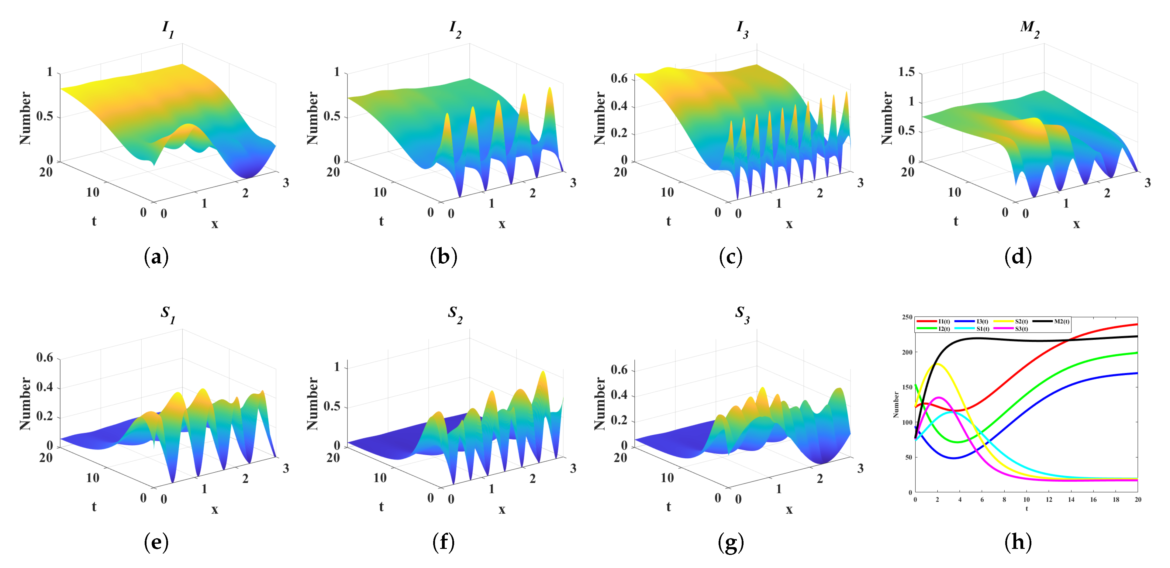
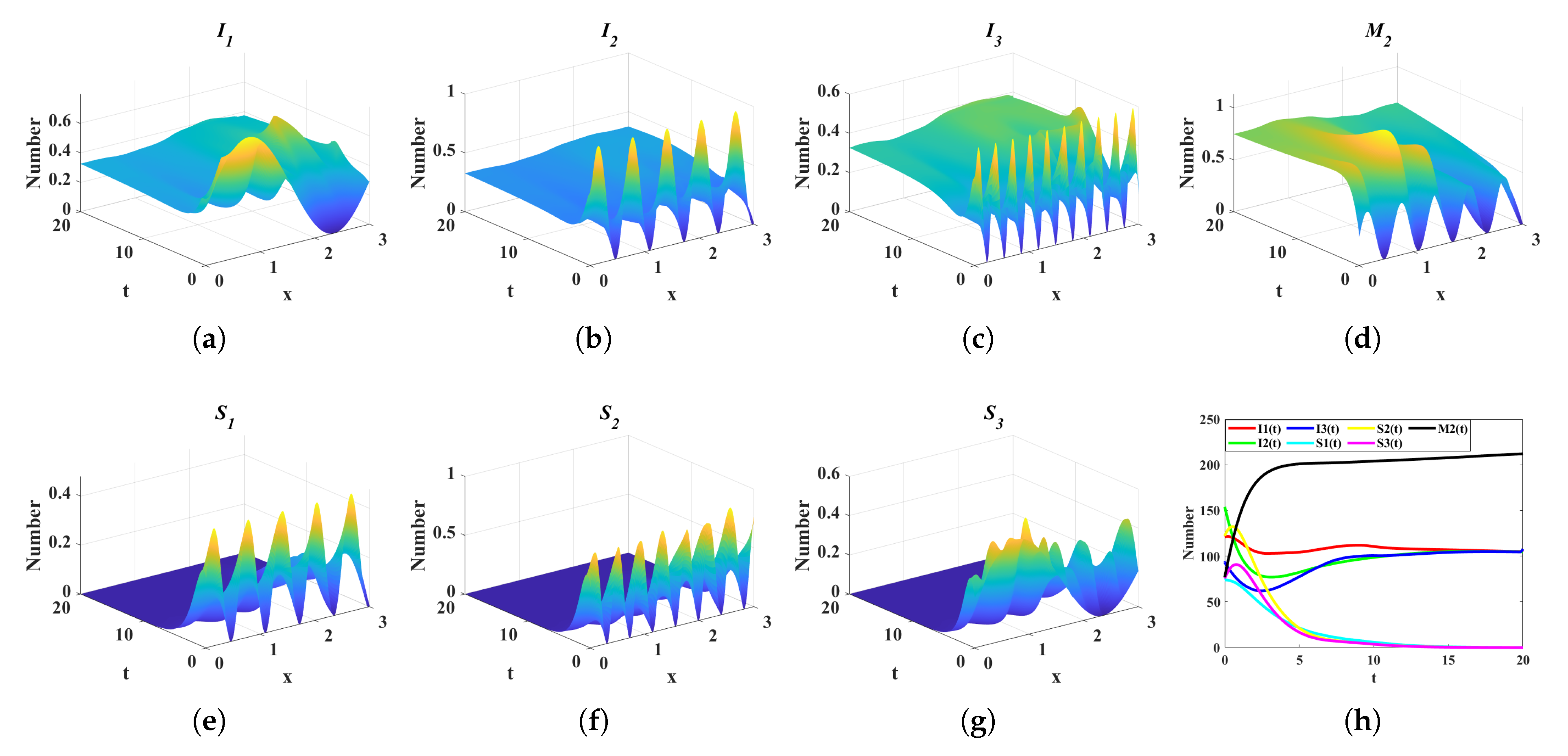
4. Numerical Simulation

In this section, simulation experiments are conducted using MATLAB R2022a to validate the theoretical results presented in Section 2 and Section 3. The experiments are divided into two parts. First, the impact of different diffusion coefficients on the control variables of rumor propagation is analyzed to verify the adaptability of the media-based spatiotemporal optimal control strategy proposed in Theorem 2. Then, the total costs of several different control strategies are compared to validate the effectiveness of the media-based spatiotemporal optimal control measures presented in Theorem 2. For simplicity, m is set to 3. In other words, the simulation environment is set for a rumor propagation scenario in three different language environments. Additionally, take ${\mathrm{\Omega }}_T=\mathrm{\Omega }\times [0,T]=[0,3]\times [0,20]$. The initial conditions are defined as follows: $I_1(x,0)=0.4(1+sin\left(2x\right)),S_1(x,0)=0.24(1+sin\left(10x\right)),D_1(x,0)=0.04(1+sin\left(5x\right)),I_2(x,0)=0.5(1+sin\left(10x\right)),S_2(x,0)=0.4(1+sin\left(15x\right)),D_2(x,0)=0.06(1+sin\left(20x\right)),I_3(x,0)=0.3(1+sin\left(20x\right)),S_3(x,0)=0.25(1+sin\left(2x\right)),D_3(x,0)=0.03(1+sin\left(6x\right))$. Other parameters are provided in the

Table 2. Parameters.

Type	Parameter	Value	Parameter	Value
Homogeneous Media Layer	$D_M$	$0.001$	${\mathrm{\Lambda }}_1$	$0.1$
	${\alpha }_1$	$0.56$	${\alpha }_2$	$0.01$
	${\mu }_1$	$0.1$
Heterogeneous Population Layer	${\mathrm{\Lambda }}_{2i},i=1,2,3$	$0.18$	${\mu }_{2i},i=1,2,3$	$0.1$
	${\gamma }_{1i},i=1,2,3$	$0.1$	${\gamma }_{2i},i=1,2,3$	$0.1$
	$D_{Pi},i=1,2,3$	$0.001$	${\beta }_1^{11}$	$0.224(1+0.4cos(x+\pi \left)\right)$
	${\beta }_1^{12}$	$0.254(1+0.4cos(x+\pi \left)\right)$	${\beta }_1^{13}$	$0.284(1+0.4cos(x+\pi \left)\right)$
	${\beta }_1^{21}$	$0.234(1+0.4cos(x+\pi \left)\right)$	${\beta }_1^{22}$	$0.264(1+0.4cos(x+\pi \left)\right)$
	${\beta }_1^{23}$	$0.294(1+0.4cos(x+\pi \left)\right)$	${\beta }_1^{31}$	$0.244(1+0.4cos(x+\pi \left)\right)$
	${\beta }_1^{32}$	$0.274(1+0.4cos(x+\pi \left)\right)$	${\beta }_1^{33}$	$0.304(1+0.4cos(x+\pi \left)\right)$
	${\beta }_2^{11}$	$0.107(1+0.4cos(x+\pi \left)\right)$	${\beta }_2^{12}$	$0.137(1+0.4cos(x+\pi \left)\right)$
	${\beta }_2^{13}$	$0.167(1+0.4cos(x+\pi \left)\right)$	${\beta }_2^{21}$	$0.117(1+0.4cos(x+\pi \left)\right)$
	${\beta }_2^{22}$	$0.147(1+0.4cos(x+\pi \left)\right)$	${\beta }_2^{23}$	$0.177(1+0.4cos(x+\pi \left)\right)$
	${\beta }_2^{31}$	$0.127(1+0.4cos(x+\pi \left)\right)$	${\beta }_2^{32}$	$0.157(1+0.4cos(x+\pi \left)\right)$
	${\beta }_2^{33}$	$0.187(1+0.4cos(x+\pi \left)\right)$	${\theta }_1$	$0.15(1+0.2cos(x+\pi \left)\right)$
	${\theta }_2$	$0.16(1+0.2cos(x+\pi \left)\right)$	${\theta }_3$	$0.17(1+0.2cos(x+\pi \left)\right)$
Cost Coefficient	$A_{1i},i=1,2,3$	1	$A_{2i},i=1,2,3$	1
	$A_3$	1	$B_{11}$	$0.4$
	$B_{12}$	$0.2$	$B_{13}$	$0.3$
	$B_{21}$	$0.001$	$B_{22}$	$0.005$
	$B_{23}$	$0.004$	$C_{1i},i=1,2,3$	1
	$C_{2i},i=1,2,3$	1	$C_3$	1

.

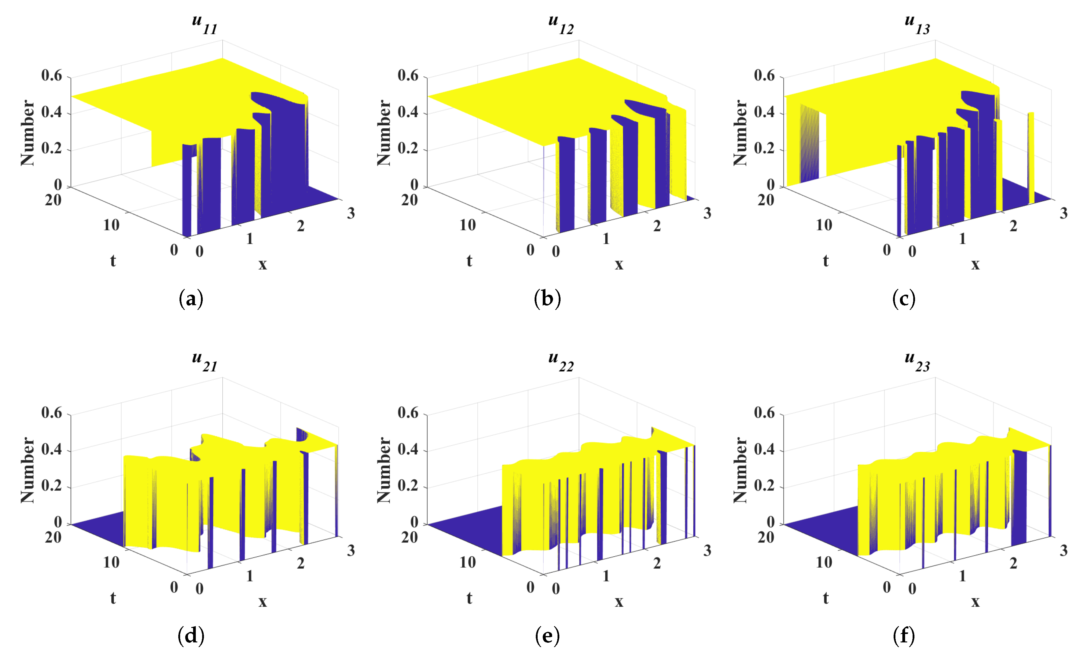
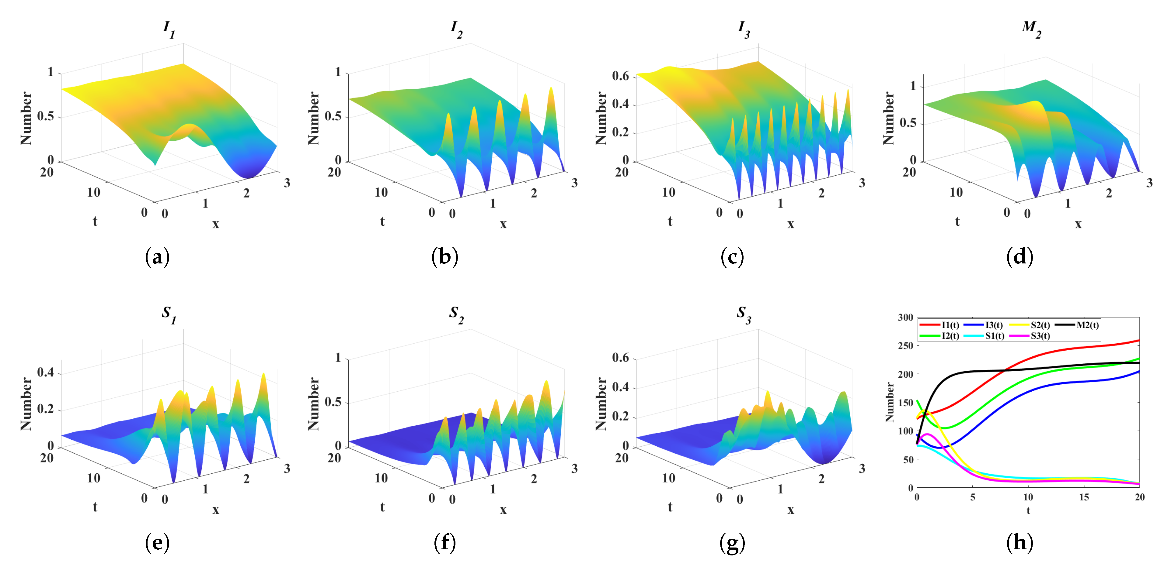
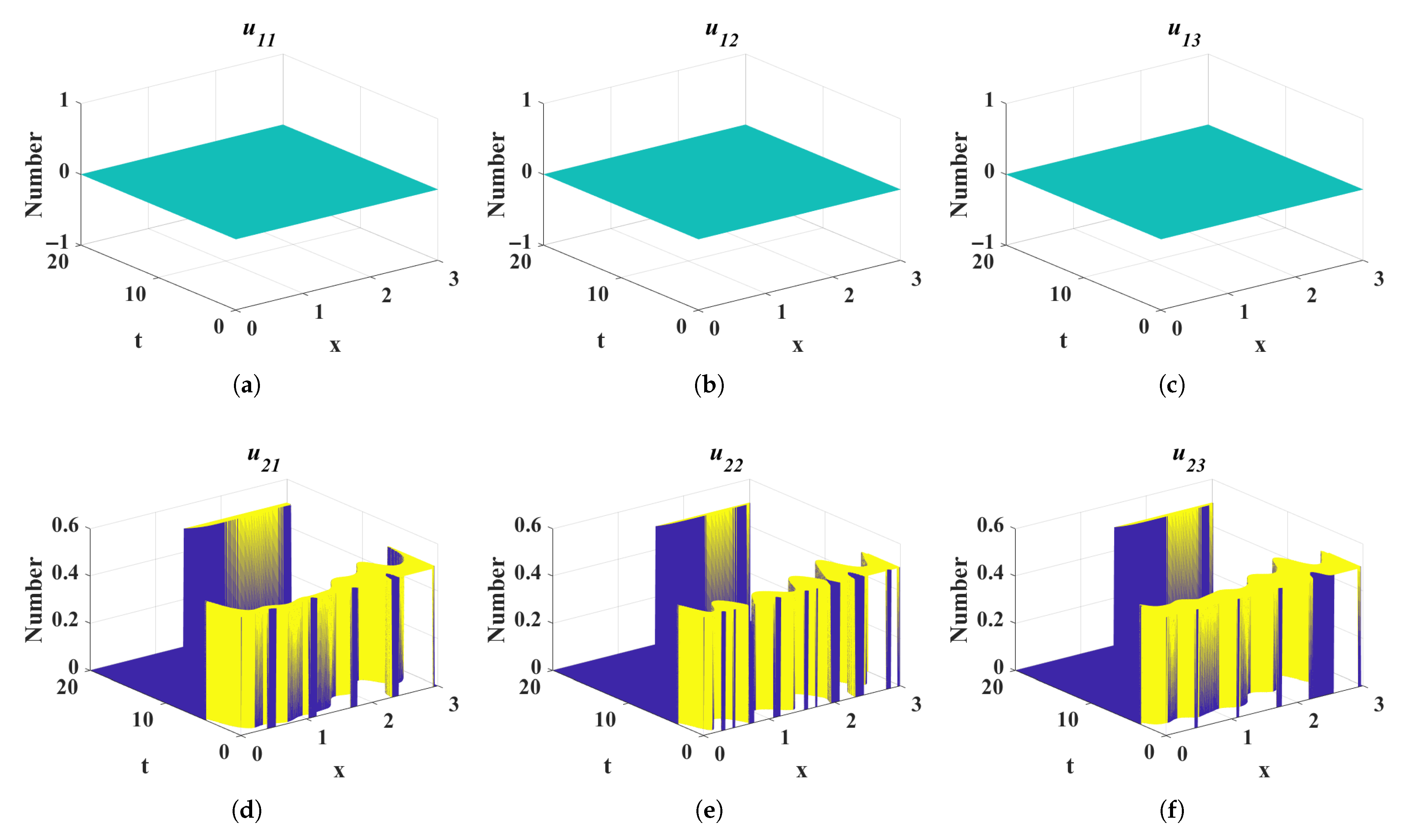
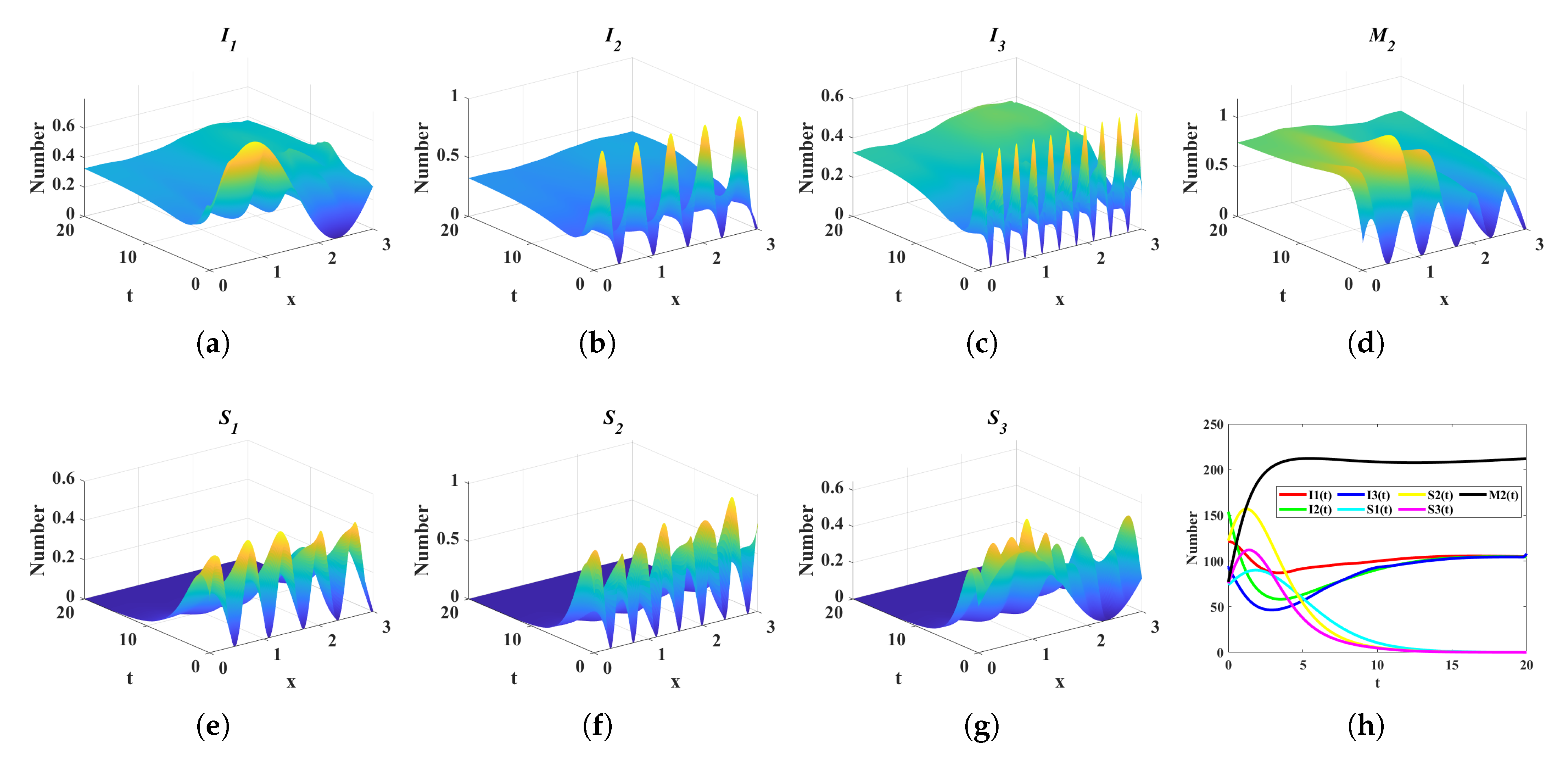
4.1. Impact of Different Diffusion Coefficients on Control Variables

Considering the varying intensities of rumor diffusion in space under different cases, it is necessary to validate the adaptability of the media-based spatiotemporal optimal control strategy proposed in Theorem 1. Next, the control strategies under three different diffusion coefficients are compared.

• Case 1:  $D_M=D_{pi}=0.001,i=1,2,3$
• Case 2:  $D_M=D_{pi}=0.005,i=1,2,3$
• Case 3:  $D_M=D_{pi}=0.01,i=1,2,3$

Other parameters are provided in Table 2. Figure 3 shows that as the diffusion coefficient increases, the control variable combinations in all three cases are dynamically adjusted. The control effects can be observed in Figure 4. Although an increase in the diffusion coefficient leads to a certain degree of growth in the total sums of the ignorant individuals $I_i$, the spreaders $S_i$, and the media platform $M_2,i=1,2,3$, across the entire region over time, they generally remain at a stable level. This indicates that the media-based spatiotemporal optimal control strategy proposed in Theorem 1 of Section 3 can dynamically adjust to adapt to different scenarios, demonstrating strong adaptability.

4.2. Comparison of Control Costs in Four Different Scenarios

The cost function reflects the media resources consumed in suppressing rumor propagation, which is often used as an important criterion for evaluating the effectiveness of an optimal control strategy. In this subsection, to validate the effectiveness of the media-based spatiotemporal optimal control strategy proposed in Theorem 1 in Section 3, we compare the cost functions of four different control strategies. The specific values of the cost functions for each scenario are provided in

Table 3. Simulation results under different scenarios.

	${\sum }_{\mathit{i}=1}^3{\mathit{A}}_{1\mathit{i}}{\mathit{I}}_{\mathit{i}}$	${\sum }_{\mathit{i}=1}^3{\mathit{A}}_{2\mathit{i}}{\mathit{S}}_{\mathit{i}}$	${\sum }_{\mathit{i}=1}^3{\mathit{B}}_{1\mathit{i}}{\mathit{u}}_{1\mathit{i}}$	${\sum }_{\mathit{i}=1}^3{\mathit{B}}_{2\mathit{i}}{\mathit{u}}_{2\mathit{i}}$	${\mathit{A}}_3{\mathit{M}}_2$	${\sum }_{\mathit{i}=1}^3{\mathit{C}}_{1\mathit{i}}{\mathit{I}}_{\mathit{i}}$	${\sum }_{\mathit{i}=1}^3{\mathit{C}}_{2\mathit{i}}{\mathit{S}}_{\mathit{i}}$	${\mathit{C}}_3{\mathit{M}}_2$	$\mathit{J}(\mathit{\vartheta },\mathit{u})$
scenario 1	85.8	31.82	0	0	41.92	6.08	0.55	2.22	168.39
scenario 2	59.57	10.83	23.24	$9.8\times {10}^{-2}$	39.51	3.19	$9.8\times {10}^{-4}$	2.12	138.56
scenario 3	91.16	24.91	0	$4.3\times {10}^{-2}$	41.39	6.05	0.52	2.22	166.29
scenario 4	54.65	17.93	24.04	0	40.42	3.18	$1.5\times {10}^{-3}$	2.12	142.34

. The corresponding parameters are provided in Table 2. The four scenarios are defined as follows:

• scenario 1: Without any control strategy ($u_{1i}\equiv 0$ and $u_{2i}\equiv 0$, $i=1,2,3$).
• scenario 2: Media debunk and prevention education control strategy ($u_{1i}\not\equiv 0$ and $u_{2i}\not\equiv 0$, $i=1,2,3$).
• scenario 3: Only media debunking control strategy ($u_{1i}\equiv 0$ and $u_{2i}\not\equiv 0$, $i=1,2,3$).
• scenario 4: Only media prevention education control strategy ($u_{1i}\not\equiv 0$ and $u_{2i}\equiv 0$, $i=1,2,3$).

scenario 1: As shown in Figure 5, in the absence of any control measures, the densities of the three categories, namely ignoramus, spreaders, and network platforms providing debunking information for rumors, evolve over time and transition from locally unstable states to a globally stable state. As indicated in Table 3, the total cost of the cost function is 168.39.

scenario 2: As shown in Figure 6, under the implementation of two control measures, the densities of the three categories, namely ignoramus and spreaders, are effectively suppressed when locally unstable, and gradually tend towards global stability over time. As indicated in Table 3, compared to Scenario 1, although the costs of the two control strategies increased by 23.34, the total density of the three types of ignoramus (I) decreased by 26.23 over the entire time period, with a decrease of 20.99 at the end of the period. The total density of the three types of spreaders (S) decreased by 2.89 over the entire time period, with a decrease of 0.54 at the end of the period. The total density of network platforms providing debunking information for rumors ($M_2$) decreased by 2.41 over the entire time period, with a decrease of 0.1 at the end of the period. The total cost decreased by 29.83. As shown in Figure 7, both types of control measures are bang–bang control strategies, further validating Remark 1.

scenario 3: As shown in Figure 8, when only the media debunking control strategy is applied, the densities of the three categories of spreaders gradually tend towards global stability over time, with the values decreasing. As indicated in Table 3, compared to Scenario 1, the cost of the control strategy increased by $4.29\times {10}^{-3}$. The total density of the three types of ignoramus (I) increased by 5.36 over the entire time period, with a decrease of 0.03 at the end of the period. The total density of the three types of spreaders (S) decreased by 6.91 over the entire time period, with a decrease of 0.03 at the end of the period. The total density of network platforms providing debunking information for rumors ($M_2$) decreased by 0.53 over the entire time period, with the total density remaining nearly unchanged at the end of the period. The total cost decreased by 2.1. As shown in Figure 9, the media debunking control strategy is a bang–bang control type, further validating Remark 1.

scenario 4: As shown in Figure 10, when only the media preventive education control strategy is applied, the densities of the three categories of ignoramus decrease significantly over time, gradually tending towards global stability, while the densities of the spreaders decrease to a lesser extent as they also tend towards global stability. As indicated in Table 3, compared to Scenario 1, the cost of the control strategy increased by 24.04. The total density of the three types of ignoramus (I) increased by 31.15 over the entire time period, with a decrease of 2.9 at the end of the period. The total density of the three types of spreaders (S) decreased by 13.89 over the entire time period, with a decrease of 0.54 at the end of the period. The total density of network platforms providing debunking information for rumors ($M_2$) decreased by 1.5 over the entire time period, with a decrease of 0.1 at the end of the period. The total cost decreased by 26.05. As shown in Figure 11, the media preventive education control strategy is a bang–bang control strategy, further validating Remark 1.

5. Conclusions

To address the challenges of predicting and controlling rumor propagation across regions and languages in real-world scenarios, this paper investigates the spatiotemporal characteristics of rumor diffusion in multilingual environments and the corresponding media-based spatiotemporal optimal control problem. Specifically, we develop a novel hybrid dual-controlled model combining a homogeneous media layer with heterogeneous population layers to characterize both the spatiotemporal dynamics and multilingual features of rumor propagation. Subsequently, we study the spatiotemporal optimal control problem of this controlled system. By proving the differentiability of the control-to-state mapping, we derive the necessary optimality conditions for the media-based control strategy. Finally, two comparative experiments demonstrate the adaptability and effectiveness of our proposed spatiotemporal media control strategy. Section 4.1 shows that the proposed optimal control strategy can adaptively adjust under different diffusion coefficients to control rumor spread among heterogeneous individuals. Section 4.2 indicates that, among four scenarios tested, Scenario 2 with two dynamic spatiotemporal control strategies yields the lowest cost function value, thereby validating the optimization performance of our optimal control strategy. Our future research will focus on integrating machine learning and reinforcement learning methods into complex reaction–diffusion systems to improve the robustness of rumor containment strategies.

References

1. Wang, J.; Liao, J.; Lu, J.G.; Li, J.; Liu, M. Dynamic Analysis of the Multi-Lingual S2IR Rumor Propagation Model Under Stochastic Disturbances. Entropy 2025, 27, 217. [Google Scholar] [CrossRef] [PubMed]
2. Li, Q.; Gao, L.; Guo, X.; Wu, X.; Wang, R.; Xiao, Y. Information Propagation Dynamic Model Based on Rumors, Antirumors, Prom-Rumors, and the Dynamic Game. IEEE Trans. Comput. Soc. Syst. 2024, 12, 376–389. [Google Scholar] [CrossRef]
3. Zhong, X.; Luo, C.; Deng, F.; Liu, G.; Li, C.; Hu, Z. Model-Based and Data-Driven Stochastic Hybrid Control for Rumor Propagation in Dual-Layer Network. IEEE Trans. Comput. Soc. Syst. 2024, 12, 777–791. [Google Scholar] [CrossRef]
4. Zhong, X.; Luo, C.; Dong, X.; Bai, D.; Liu, G.; Xie, Y.; Peng, Y. Stochastic Stabilization of Dual-Layer Rumor Propagation Model with Multiple Channels and Rumor-Detection Mechanism. Entropy 2023, 25, 1192. [Google Scholar] [CrossRef]
5. Liao, J.; Wang, J.; Li, J.; Jiang, X. The Dynamics and Control of a Multi-Lingual Rumor Propagation Model with Non-Smooth Inhibition Mechanism. Math. Biosci. Eng. 2024, 21, 5068–5091. [Google Scholar] [CrossRef]
6. Xia, Y.; Jiang, H.; Yu, Z.; Yu, S.; Luo, X. Dynamic Analysis and Optimal Control of a Reaction-Diffusion Rumor Propagation Model in Multi-Lingual Environments. J. Math. Anal. Appl. 2023, 521, 126967. [Google Scholar] [CrossRef]
7. Chong, S.K.; Ali, S.H.; Ðoàn, L.N.; Yi, S.S.; Trinh-Shevrin, C.; Kwon, S.C. Social Media Use and Misinformation Among Asian Americans During COVID-19. Front. Public Health 2022, 9, 764681. [Google Scholar] [CrossRef]
8. Zhong, X.; Zheng, Y.; Xie, J.; Xie, Y.; Peng, Y. Multi-Agent Collaborative Rumor-Debunking Strategies on Virtual-Real Network Layer. Mathematics 2024, 12, 462. [Google Scholar] [CrossRef]
9. Huo, L.; Chen, S.; Zhao, L. Dynamic Analysis of the Rumor Propagation Model with Consideration of the Wise Man and Social Reinforcement. Physica A 2021, 571, 125828. [Google Scholar] [CrossRef]
10. Zhong, X.; Zhang, J.; Wang, A.; Liu, G.; Deng, F.; Wang, J. Rumor Suppression in a Three-Layer Network: A Reinforcement Learning Algorithm. IEEE Trans. Netw. Sci. Eng. 2025, 12, 2292–2307. [Google Scholar] [CrossRef]
11. Wang, J.; Jiang, H.; Hu, C.; Yu, Z.; Li, J. Stability and Hopf Bifurcation Analysis of Multi-Lingual Rumor Spreading Model with Nonlinear Inhibition Mechanism. Chaos Solitons Fractals 2021, 153, 111464. [Google Scholar] [CrossRef]
12. Gan, C.; Yang, W.; Zhu, Q.; Li, M.; Jain, D.K.; Štruc, V.; Huang, D.W. Hybrid Rumor Debunking in Online Social Networks: A Differential Game Approach. IEEE Trans. Syst. Man Cybern. Syst. 2025, 55, 2513–2527. [Google Scholar] [CrossRef]
13. Pan, Y.; Shen, S.; Zhu, L. Spatio-Temporal Pattern Formation Mechanism of an Epidemic-Like Information Propagation Model with Diffusion Behavior. Ain Shams Eng. J. 2025, 16, 103244. [Google Scholar] [CrossRef]
14. Zhu, L.; Huang, X.; Liu, Y.; Zhang, Z. Spatiotemporal Dynamics Analysis and Optimal Control Method for an SI Reaction-Diffusion Propagation Model. J. Math. Anal. Appl. 2021, 493, 124539. [Google Scholar] [CrossRef]
15. Hu, J.; Zhu, L. Turing Pattern Analysis of a Reaction-Diffusion Rumor Propagation System with Time Delay in Both Network and Non-Network Environments. Chaos Solitons Fractals 2021, 153, 111542. [Google Scholar] [CrossRef]
16. Ke, Y.; Zhu, L.; Wu, P.; Shi, L. Dynamics of a Reaction-Diffusion Rumor Propagation Model with Non-Smooth Control. Appl. Math. Comput. 2022, 435, 127478. [Google Scholar] [CrossRef]
17. Huo, L.; Dong, Y. Dynamics and Near-Optimal Control in a Stochastic Rumor Propagation Model Incorporating Media Coverage and Lévy Noise. Chin. Phys. B 2022, 31, 030202. [Google Scholar] [CrossRef]
18. Chang, Z.; Jiang, H.; Yu, S.; Chen, S. Dynamic Analysis and Optimal Control of ISCR Rumor Propagation Model with Nonlinear Incidence and Time Delay on Complex Networks. Discrete Dyn. Nat. Soc. 2021, 2021, 3935750. [Google Scholar] [CrossRef]
19. Liu, G.; Tan, Z.; Liang, Z.; Chen, H.; Zhong, X. Fractional optimal control for malware propagation in Internet of Underwater Things. IEEE Internet Things J. 2024, 11, 11632–11651. [Google Scholar] [CrossRef]
20. Liu, G.; Li, H.; Xiong, L.; Tan, Z.; Liang, Z.; Zhong, X. Fractional order optimal control and FIov–MASAC reinforcement learning for combating malware spread in Internet of Vehicles. IEEE Trans. Autom. Sci. Eng. 2025, 22, 10313–10332. [Google Scholar] [CrossRef]
21. Liu, G.; Xu, H.; Zhang, J.; Liang, Z.; Zhong, X. Spatiotemporal Control Optimization of Malware Propagation in Internet of Underwater Things. IEEE Trans. Inf. Forensics Secur. 2025, 20, 6324–6339. [Google Scholar] [CrossRef]
22. Liu, G.; Xu, H.; Wang, K.; Bai, D.; Liang, Z. Spatiotemporal Optimal Control of Reaction-Diffusion Malware Propagation in Multi-AUV Networks. IEEE Trans. Netw. Sci. Eng. 2025. early access. [Google Scholar] [CrossRef]
23. Liu, G.; Xu, H.; Zhang, J.; Zhong, X.; Liang, Z. Spatiotemporal Optimal Control of Malware Propagation in AUV-Assisted UWSNs: A Two-Layer Heterogeneous Network. IEEE Internet Things J. 2025. early access. [Google Scholar] [CrossRef]
24. Zhong, X.; Luo, C.; Zhang, J.; Liu, G. Higher-order rumor and anti-rumor propagation and data-driven optimal control on hypergraphs. Chaos Solitons Fractals 2025, 193, 116082. [Google Scholar] [CrossRef]
25. Liu, G.; Zhang, J.; Zhong, X.; Hu, X.; Liang, Z. Hybrid optimal control for malware propagation in UAV–WSN system: A stacking ensemble learning control algorithm. IEEE Internet Things J. 2024, 11, 36549–36568. [Google Scholar] [CrossRef]
26. Yang, Y.; Liu, G.; Liang, Z.; Chen, H.; Zhu, L.; Zhong, X. Hybrid control for malware propagation in rechargeable WUSN and WASN: From knowledge-driven to data-driven. Chaos Solitons Fractals 2023, 173, 113703. [Google Scholar] [CrossRef]
27. Zhou, M.; Xiang, H.; Li, Z. Optimal control strategies for a reaction–diffusion epidemic system. Nonlinear Anal. Real World Appl. 2019, 46, 446–464. [Google Scholar] [CrossRef]
28. Wang, J.; Zhao, H. Threshold dynamics and regional optimal control of a malaria model with spatial heterogeneity and ivermectin therapy. Appl. Math. Model. 2024, 125, 591–624. [Google Scholar] [CrossRef]
29. Dai, F.; Liu, B. Optimal control problem for a general reaction-diffusion eco-epidemiological model with disease in prey. Appl. Math. Model. 2020, 88, 1–20. [Google Scholar] [CrossRef]
30. Bouissa, A.; Tahiri, M.; Tsouli, N.; Ammi, M.R.S. Optimal control of multi-group spatio-temporal SIR model. J. Math. Anal. Appl. 2025, 542, 128835. [Google Scholar] [CrossRef]
31. Zhou, M.; Xiang, H. Optimal control problems of a reaction–diffusion ecological model with a protection zone. J. Process Control 2022, 120, 97–114. [Google Scholar] [CrossRef]
32. Apreutesei, N.C. An optimal control problem for a pest, predator, and plant system. Nonlinear Anal. Real World Appl. 2012, 13, 1391–1400. [Google Scholar] [CrossRef]
Figure 1. The methodological framework of this paper.
Mathematics 13 02253 g001
Figure 2. State transitions at time t.
Mathematics 13 02253 g002
Figure 3. Temporal evolution of the total spatial sum of control variable intensities under three different diffusion coefficients. (a) Temporal evolution of the state variable u 11 . (b) Temporal evolution of the state variable u 12 . (c) Temporal evolution of the state variable u 13 . (d) Temporal evolution of the state variable u 21 . (e) Temporal evolution of the state variable u 22 . (f) Temporal evolution of the state variable u 23 . (The temporal evolution of the control variable represents the total control intensity, aggregated over the spatial domain from x = 0 to x = 3 , at each time point).
Mathematics 13 02253 g003
Figure 4. Temporal evolution of the total spatial sum of state variables under the media-based spatiotemporal control strategy for three different diffusion coefficients. (a) Temporal evolution of the state variable I 1 . (b) Temporal evolution of the state variable I 2 . (c) Temporal evolution of the state variable I 3 . (d) Temporal evolution of the state variable S 1 . (e) Temporal evolution of the state variable S 2 . (f) Temporal evolution of the state variable S 3 . (g) Temporal evolution of the state variable M 2 . (The temporal evolution of the state variable represents the total state density, integrated over the spatial domain from x = 0 to x = 3 , at each time point.
Mathematics 13 02253 g004
Figure 5. Dynamic evolution of state variables under scenario 1. (a) Spatiotemporal evolution of the ignoramus I 1 . (b) Spatiotemporal evolution of the ignoramus I 2 . (c) Spatiotemporal evolution of the ignoramus I 3 . (d) Spatiotemporal evolution of the media platform M 2 . (e) Spatiotemporal evolution of the spreaders S 1 . (f) Spatiotemporal evolution of the spreaders S 2 . (g) Spatiotemporal evolution of the spreaders S 3 . (h) Temporal evolution of the total spatial sum of densities for state variables I 1 , I 2 , I 3 , M 2 , S 1 , S 2 and S 3 . (The spatiotemporal evolution of the state variable describes the dynamic variation of its density across the temporal interval t = 0 to t = 20 and the spatial domain x = 0 to x = 3 ).
Mathematics 13 02253 g005
Figure 6. Dynamic evolution of state variables under scenario 2. (a) Spatiotemporal evolution of the ignoramus I 1 . (b) Spatiotemporal evolution of the ignoramus I 2 . (c) Spatiotemporal evolution of the ignoramus I 3 . (d) Spatiotemporal evolution of the media platform M 2 . (e) Spatiotemporal evolution of the spreaders S 1 . (f) Spatiotemporal evolution of the spreaders S 2 . (g) Spatiotemporal evolution of the spreaders S 3 . (h) Temporal evolution of the total spatial sum of densities for state variables I 1 , I 2 , I 3 , M 2 , S 1 , S 2 and S 3 . (The spatiotemporal evolution of the state variable describes the dynamic variation of its density across the temporal interval t = 0 to t = 20 and the spatial domain x = 0 to x = 3 ).
Mathematics 13 02253 g006
Figure 7. Dynamic evolution of control variables under scenario 2. (a) Spatiotemporal evolution of media preventive education measure u 11 . (b) Spatiotemporal evolution of media preventive education measure u 12 . (c) Spatiotemporal evolution of media preventive education measure u 13 . (d) Spatiotemporal evolution of media debunking control strategy u 21 . (e) Spatiotemporal evolution of media debunking control strategy u 22 . (f) Spatiotemporal evolution of media debunking control strategy u 23 . (The spatiotemporal evolution of the control variable describes the dynamic variation of its density across the temporal interval t = 0 to t = 20 and the spatial domain x = 0 to x = 3 ).
Mathematics 13 02253 g007
Figure 8. Dynamic evolution of state variables under scenario 3. (a) Spatiotemporal evolution of the ignoramus I 1 . (b) Spatiotemporal evolution of the ignoramus I 2 . (c) Spatiotemporal evolution of the ignoramus I 3 . (d) Spatiotemporal evolution of the media platform M 2 . (e) Spatiotemporal evolution of the spreaders S 1 . (f) Spatiotemporal evolution of the spreaders S 2 . (g) Spatiotemporal evolution of the spreaders S 3 . (h) Temporal evolution of the total spatial sum of densities for state variables I 1 , I 2 , I 3 , M 2 , S 1 , S 2 , and S 3 . (The spatiotemporal evolution of the control variable describes the dynamic variation of its density across the temporal interval t = 0 to t = 20 and the spatial domain x = 0 to x = 3 .)
Mathematics 13 02253 g008
Figure 9. Dynamic evolution of control variables under scenario 3. (a) Spatiotemporal evolution of media preventive education measure u 11 . (b) Spatiotemporal evolution of media preventive education measure u 12 . (c) Spatiotemporal evolution of media preventive education measure u 13 . (d) Spatiotemporal evolution of media debunking control strategy u 21 . (e) Spatiotemporal evolution of media debunking control strategy u 22 . (f) Spatiotemporal evolution of media debunking control strategy u 23 . (The spatiotemporal evolution of the control variable describes the dynamic variation of its density across the temporal interval t = 0 to t = 20 and the spatial domain x = 0 to x = 3 ).
Mathematics 13 02253 g009
Figure 10. Dynamic evolution of state variables under scenario 4. (a) Spatiotemporal evolution of the ignoramus I 1 . (b) Spatiotemporal evolution of the ignoramus I 2 . (c) Spatiotemporal evolution of the ignoramus I 3 . (d) Spatiotemporal evolution of the media platform M 2 . (e) Spatiotemporal evolution of the spreaders S 1 . (f) Spatiotemporal evolution of the spreaders S 2 . (g) Spatiotemporal evolution of the spreaders S 3 . (h) Temporal evolution of the total spatial sum of densities for state variables I 1 , I 2 , I 3 , M 2 , S 1 , S 2 , and S 3 . (The spatiotemporal evolution of the control variable describes the dynamic variation of its density across the temporal interval t = 0 to t = 20 and the spatial domain x = 0 to x = 3 ).
Mathematics 13 02253 g010
Figure 11. Dynamic evolution of control variables under scenario 4. (a) Spatiotemporal evolution of media preventive education measure u 11 . (b) Spatiotemporal evolution of media preventive education measure u 12 . (c) Spatiotemporal evolution of media preventive education measure u 13 . (d) Spatiotemporal evolution of media debunking control strategy u 21 . (e) Spatiotemporal evolution of media debunking control strategy u 22 . (f) Spatiotemporal evolution of media debunking control strategy u 23 . (The spatiotemporal evolution of the control variable describes the dynamic variation of its density across the temporal interval t = 0 to t = 20 and the spatial domain x = 0 to x = 3 ).
Mathematics 13 02253 g011