A Deep Learning-Driven Solution to Limited-Feedback MIMO Relaying Systems

Abstract

In this work, we investigate a new design strategy for the implementation of a deep neural network (DNN)-based limited-feedback relay system by using conventional filters to acquire training data in order to jointly solve the issues of quantization and feedback. We aim to maximize the effective channel gain to reduce the symbol error rate (SER). By harnessing binary feedback information from the implemented DNNs together with efficient beamforming vectors, a novel approach to the resulting problem is presented. We compare our proposed system to a Grassmannian codebook system to show that our system outperforms its benchmark in terms of SER.

1. Introduction

Limited-feedback systems have been studied widely with the aim of improving the performance of closed-loop communication under frequency-division duplexing (FDD) [1,2]. The generic models adopt two stages of communication which involve (i) channel estimation (CE) via pilot signals and (ii) the received pilot signal quantization and feedback of the codebook index of the estimated channel to the transmitter for successive transmissions [3,4].

Recognizing the vital role that codebooks play in closed-loop systems, studies on limited feedback systems have focused on improving the design of codebooks to optimize channel estimation, quantization, and the index feedback chain [5]. The Grassmannian, Lloyd, and discrete Fourier transform (DFT)-based codebook designs are among the results of such attempts [1,6]. Predominant among the optimization parameters in the literature is the chordal distance criterion.

In [7], the authors proposed a new Grassmannian-based approach to massive multiple-input multiple-output (MIMO) two-tier system designs in order to facilitate limited feedback communication. Vital to their codebooks is the problem of estimating the channel state information (CSI). Nevertheless, solving that problem together with codebook quantization is non-convex due to the highly combinatorial nature of the joint problem [8,9].

To extend transmission range, MIMO systems turn to relays [10,11]. The MIMO relay system in [12] relies on Wiener filter-based techniques to present a new design strategy as a competitor to traditional singular value decomposition (SVD)-based approaches. Their approach seeks to optimize the computation of the minimum mean-squared error (MMSE). In [13], the use of an improved adaptive codebook channel estimation method was investigated to exploit multi-carrier parameters in its CE and feedback attempts.

However, the same non-joint problem exists in the systems studied in [12,13]; channel quantization and channel estimation are each solved independently, which is suboptimal. Another problem is that MIMO relay systems only use single feedback links. These links exist either as destination-to-relay or destination-to-source. Neither the inter-relay (for multi-relay cases) or transmitter-to-relay links have their feedback channels considered. Hence, both channel estimation and quantization are not performed on the neglected links. Recent works [8,14] have attempted a joint solution using MIMO relay feedback systems with deep neural networks (DNNs) and deep learning (DL), respectively, while Refs. [8,14] consider only point-to-point MIMO systems. To the best of our knowledge, no other work has considered joint CE and quantization for limited-feedback MIMO relay systems using DNN [15].

Motivated by the above, this paper considers a MIMO relay system with limited feedback using DNN. Specifically, we focus on the joint CE and quantization solution in a dual-hop limited feedback chain of a MIMO relay system using DNNs. Consequently, our system is expected to react better in more dynamic real-world situations where the channel is changing constantly and where the assumption of perfect CSI becomes unrealistic. The main contributions of this paper are as follows: (i) the introduction of a dual-hop DNN-driven limited-feedback MIMO relaying system that offers significant gain over existing conventional and codebook-based limited feedback MIMO relay systems, and (ii) the joint solution for the CE and quantization phases in an amplify-and-forward (AF) MIMO relaying system via DNN.

The rest of this paper is organized as follows: Section 2 presents the system model and problem formulation; the implementation of the DNN-based system is provided in Section 3; Section 4 presents the simulation results and analysis; finally, our conclusions are provided in Section 5.

Notation: $\mathbf{A}\in {\mathbb{C}}^{N\times M}$ denotes a matrix with dimensions N by M; ${\mathbb{Z}}^{*}$ indicates the set of integers comprising 1 and $-1$; $\mathrm{tr}\left\{\mathbf{A}\right\}$ and ${\mathbf{A}}^{†}$ represent the trace and conjugate transpose of matrix $\mathbf{A}$, respectively; estimations of matrix $\mathbf{A}$ and vector $\mathbf{a}$ are presented as $\widehat{\mathbf{A}}$ and $\widehat{\mathbf{a}}$, respectively; $\left|\mathbf{A}\right|$ and $\left|\right|\mathbf{A}\left|\right|$ are the determinant and the norm of $\mathbf{A}$, respectively; ${\mathbf{I}}_N$ denotes an N × N identity matrix; $n\sim \mathcal{CN}(0,{\delta }^2)$ denotes a circularly symmetric complex Gaussian random variable n with zero mean and variance ${\delta }^2$; ${\mathbb{E}}_X\left[f\left(X\right)\right]$ is the expectation operation over random variable X; $\Re \left\{·\right\}$ and $\Im \left\{·\right\}$ correspond to the real and imaginary components, respectively; $\mathrm{vec}\left(·\right)$ and $\mathrm{diag}\left(·\right)$ represent the vectorization and diagonalization operations, respectively.

2. System Model and Problem Formulation

We consider a scenario in which a source node communicates with its destination node through a relay node by using a dual-hop limited-feedback chain, as shown in Figure 1. The main DNN layers located at each node, and their roles are summarized in

Table 1. Main DNN layers present at nodes and their roles.

Nodal Components and Roles
Component	S	R	D	Role
Fully Connected Layers (FCL)	✓	✓	✓	combines features from previous layer into single vector
Multiple Fully Connected Layers (MFCL)	✓	✓	✓	a chain of ReLU activated FCLs
Binarization	✗	✗	✓	Removes combinatorial constraint of (13)

. The source, relay, and destination nodes are equipped with antennas, denoted $N_t,N_r$, and $N_d$, respectively. In addition, $N_s$ represents the number of streams. We assume that there is no direct path between the source and destination due to high path loss and shadowing. We define the channels from the source to the relay as ${\mathbf{H}}_{RT}\in {\mathbb{C}}^{N_r\times N_t}$ and from the relay to the destination as ${\mathbf{H}}_{DR}\in {\mathbb{C}}^{N_d\times N_r}$.

Phase 1 of Figure 1 is made up of two main stages, with stage 1 being all pilot selection instances and stage 2 being all data transmission occurrences; any feedback process falls under phase 2. First, the pilot signal ${\mathbf{p}}_S$ is sent from the transmitter to the relay in order to estimate the channel ${\mathbf{H}}_{RT}$. The optimal precoding matrix index (PMI) $i_2^{*}$ [16,17] of the estimated channel ${\widehat{\mathbf{H}}}_{RT}$ is then fed back to the transmitter from the relay; see Figure 1. The index $i_2^{*}$ is used to select the transmit precoder, from a predefined codebook $\mathcal{C}=\left\{{\mathbf{c}}_1,{\mathbf{c}}_2,\dots ,{\mathbf{c}}_{2^B}\right\}$ for the transmission of the precoded symbol ${\mathbf{s}}_s={\mathbf{c}}_{S}x$ to the relay. Here, B denotes the total feedback bits, which also determines the size of $\mathcal{C}$. Note that in the DNN the vectors ${\mathbf{b}}_R\in {\mathbb{Z}}^{*B\times 1}$ and ${\mathbf{b}}_D\in {\mathbb{Z}}^{*B\times 1}$ are considered independent but equivalent characterizations of indices $i_2^{*}$ and $i_1^{*}$ from the relay and destination, respectively. In the case of the transmitter DNN, the unit norm vector ${\mathbf{c}}_S\in {\mathbb{C}}^{N_t\times 1}$ is constructed from ${\mathbf{b}}_R$ to maximize the effective channel gain in (3). The signal at the relay is provided as follows [12,18]:

$$\begin{array}{cc}\hfill {\mathbf{y}}_R& =\sqrt{E_s}{\mathbf{l}}_R{\mathbf{H}}_{RT}{\mathbf{s}}_s+{\mathbf{l}}_R{\mathbf{n}}_R\hfill \end{array}$$

(1)

where ${\mathbf{l}}_R\in {\mathbb{C}}^{1\times N_r}$ denotes the relay receive filter, while $\sqrt{E_s}$ and ${\mathbf{n}}_R\in {\mathbb{C}}^{N_r\times 1}\sim \mathcal{CN}\left(\mathbf{0},{\sigma }_{n_R}^2{\mathbf{I}}_{N_r}\right)$ indicate the source’s symbol transmit energy and noise vector signal at the relay, respectively. We also assume an amplify-and-forward protocol in our transmissions.

Similarly, R sends the pilot signal ${\mathbf{p}}_R$ to D in order to estimate ${\mathbf{H}}_{DR}$. The resulting channel estimate ${\widehat{\mathbf{H}}}_{DR}$ from the destination filtering (2) is used to select the corresponding index $i_1^{*}$, also selected from codebook $\mathcal{C}$, for feedback to R. The received signal at the destination is expressed as

$$\begin{array}{cc}\hfill {\mathbf{y}}_D& =\sqrt{E_r}{\mathbf{H}}_{DR}{\mathbf{c}}_R\left(\sqrt{E_s}{\mathbf{l}}_R{\mathbf{H}}_{RT}{\mathbf{s}}_s+{\mathbf{l}}_R{\mathbf{n}}_R\right)+{\mathbf{n}}_D,\hfill \end{array}$$

(2)

where ${\mathbf{n}}_D\in {\mathbb{C}}^{N_d\times 1}$ and ${\mathbf{c}}_R\in {\mathbb{C}}^{N_r\times 1}$ identify the noise at the destination and the relay precoder, respectively, while $\sqrt{E_r}$ represents the symbol transmit energy. The elements of ${\mathbf{n}}_D$ are modeled as $\mathcal{CN}\left(\mathbf{0},{\sigma }_{n_D}^2{\mathbf{I}}_{N_d}\right)$.

Conventionally, the optimization of the CE and feedback processes are highly combinatorial and non-convex [8,19], and as such are solved separately, leading to suboptimal solutions. Thus, in Section 2.2 we introduce a limited-feedback design in which DNNs replace both the CE and quantized feedback stages (see the incorporated DNN layers at each node of the dashed boxes in Figure 1). Using a DNN, we unite the two problems into one in order to offer a joint solution. Therefore, the proposed system envisions a two-phase training/machine learning (ML) lead chain primed on a DNN, which offers an approach to jointly optimize our limited-feedback system.

2.1. Conventional Approach

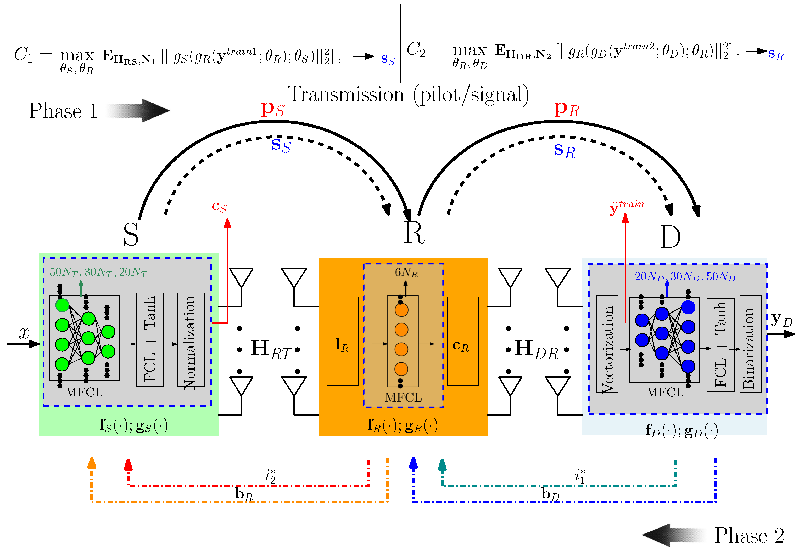
The optimal PMI indices $i_1^{*}$ and $i_2^{*}$ obtained in the piloting stage are used to select the precoders ${\mathbf{c}}_R$ and ${\mathbf{c}}_S$, respectively, from the codebook of interest for stage 2 of phase 1. The optimal PMI is chosen by solving for the effective channel gain as

$$\begin{array}{cc}\hfill i^{*}& =\underset{i\in \{1,\dots ,2^B\}}{\mathrm{argmax}}\left|\right|{\widehat{\mathbf{H}}}_{\xi }{\mathbf{c}}_i{\left|\right|}_2^2,\hfill \end{array}$$

(3)

where $\xi \in \left\{RT,DR\right\}$, ${\mathbf{c}}_i$ is the i-th vector selected from the codebook $\mathcal{C}$, and $\widehat{\mathbf{H}}$ denotes the channel estimate. The obtained $i^{*}$ is then sent through the feedback channel to the preceding node for codebook selection and precoding. We rewrite (3) as follows:

$$\begin{array}{c}\hfill \underset{i_1^{*},i_2^{*}}{\mathrm{argmax}}{\mathbb{E}}_{{\mathbf{H}}_{RT},{\mathbf{H}}_{DR}}\left[\left|\right|{\mathbf{H}}_{DR}·{\mathbf{c}}_R^{i_1^{*}}{\left|\right|}^2·\left|\right|{\mathbf{H}}_{RT}·{\mathbf{c}}_S^{i_2^{*}}{\left|\right|}^2\right].\end{array}$$

(4)

Note that ${\mathbf{c}}_R^{i_1^{*}}$ and ${\mathbf{c}}_S^{i_2^{*}}$ here represent the selection of precoders from the indicated codebook based on the corresponding index. We adopt a system that uses a Grassmannian codebook as a benchmark against our system [20]. For all transmissions, we assume a maximum ratio transmission (MRT) scheme, while all receiving uses maximum ratio combining (MRC) filters (i.e., at both the relay and receiver sides).

2.2. DNN Approach

Unlike the conventional method, the DNN method jointly considers the processes of CE and limited feedback. Again, we consider two main phases. During phase 1 (modeled by (5)), two training sets ${\mathbf{Y}}_R^{train}$ and ${\mathbf{Y}}_D^{train}$ are formed for the DNN layers at R and D, respectively. The training sets consist of the transmission and aggregation of pilot signals.

In phase 2, training occurs at R and D using training sets ${\mathbf{Y}}_R^{train}$ and ${\mathbf{Y}}_D^{train}$. The training at R and D results in bipolar vectors ${\mathbf{b}}_R$ and ${\mathbf{b}}_D$, respectively; see Figure 1. The two vectors are understood as equivalent representations of $i_2^{*}$ and $i_1^{*}$ found in the conventional scheme. For maximum effective channel gain, they are employed to construct their respective equivalent unit-norm beamforming vectors at the source and relay, respectively, within our DNN system. Thus, the DNN is utilized for both joint CE and quantization. Three different DNN layers are implemented at the transmitter, relay, and destination which have respective mappings of $g_S\left(·\right),g_R\left(·\right)$, and $g_D\left(·\right)$ [8]. The three mappings correspond positionally to the conventional codebook selection functions, denoted as $f_S\left(·\right),f_R\left(·\right)$, and $f_D\left(·\right)$. Next, we provide a detailed description of phases 1 and 2.

2.2.1. Pilot Signal Modeling and Aggregation

We propose a DL structure for the limited-feedback system illustrated in Figure 1. The signal received at the destination is provided by redefining (2) as ${\mathbf{y}}_l^{train}$, where

$$\begin{array}{cc}\hfill {\mathbf{y}}_l^{train}& =\sqrt{E_R}{\mathbf{p}}_S{\mathbf{H}}_{DR}\left(\sqrt{E_S}{\mathbf{l}}_R{\mathbf{H}}_{RT}{\mathbf{p}}_l+{\mathbf{l}}_R{\mathbf{n}}_{R_l}\right)+{\mathbf{n}}_{D_l},\hfill \end{array}$$

(5)

$\forall l=\left\{1,2,\dots ,L\right\}$, where L represents the total number of pilot instances and where ${\mathbf{n}}_{R_l}\in {\mathbb{C}}^{N_r\times 1}$ and ${\mathbf{n}}_{D_l}\in {\mathbb{C}}^{N_d\times 1}$ denote the noise vectors at the relay and destination, respectively, for pilot transmission l. As such, the matrix $\mathbf{P}\triangleq \left[{\mathbf{p}}_1,{\mathbf{p}}_2,\dots ,{\mathbf{p}}_L\right]\in {\mathbb{C}}^{N_t\times L}$ indicates all the signal vectors used in pilot transmission with ${\mathbf{p}}_l\triangleq {\mathbf{F}}_{T}x$; the pilot signal is generated using the normalized discrete Fourier transform codebook outlined in Table I of [21]. These L instances of the ${\mathbf{y}}_l^{train}$ pilot train transmissions are aggregated into a matrix as ${\mathbf{Y}}^{train}\triangleq \left\{{\mathbf{y}}_1^{train},{\mathbf{y}}_2^{train},\dots ,{\mathbf{y}}_L^{train}\right\}$ to form a dataset. The resulting dataset is vectorized using the $\mathrm{vec}(·)$ function. Afterwards, the real and imaginary parts of the complex vector dataset are partitioned by using the $\mathrm{split}(·)$ function [8] to form ${\tilde{\mathbf{y}}}^{train}$. Thus, we have

$$\begin{array}{cc}\hfill \mathrm{split}\left(\mathrm{vec}\left({\mathbf{Y}}^{train}\right)\right)& ={\tilde{\mathbf{y}}}^{train}\hfill \\ \hfill {\tilde{\mathbf{y}}}^{train}& =[\Re \left\{{\mathbf{y}}^{train}\right\},\Im \left\{{\mathbf{y}}^{train}\right\}]\hfill \end{array}$$

(6)

as the new training set. Next, the data are preprocessed and readied for phase 2 of training and feedback through the DNN.

2.2.2. DNN Training and Learning

The preprocessed ${\mathbf{Y}}_{train}$ dataset from (6) is fed into the DNN. The DNNs employed at S, R, and D have mappings $g_S(·),g_R(·),\mathrm{and}{g}_D(·)$, respectively; see Figure 1. The destination DNN comprises three main layers, with each having a dense input layer, a batch normalizer, and an activation function (i.e., a rectified linear unit (ReLU)). The three dense input layers of the three main groups have dimensions $K_{D_1}=50N_t,K_{D_2}=30N_t$, and $K_{D_3}=20N_t$, respectively. Hence, the output of the first set’s dense layer is fed into its batch normalizer and the resulting output is also fed into its ReLU activator to provide the first layer’s output. That output is then fed as input into the second layer’s set of modules, with the input dense layer dimension set as $30N_t$. The second layer’s output is then fed into the final set with dimension $50N_t$. Similarly, the relay provided by $g_R(·)$ is made up of a single set of layers and has dimensions $6N_R$. Finally, the DNN at node S completes the final link of the DNN-modeled limited feedback link. This is a model with a set of modules similar to that of the receiver; however, its dimensions are in reverse order to that of the receiver, that is, $50N_D$ for set one, $30N_D$ for set two, and finally $20N_D$.

The various mappings in the proposed limited-feedback MIMO relay system are described as follows. At D, the optimal PMI which maximizes the effective channel gain over ${\widehat{\mathbf{H}}}_{RT}$ and ${\widehat{\mathbf{H}}}_{DR}$ (provided by (3)) is realized as the bipolar vector ${\mathbf{b}}_D=g_D({\tilde{\mathbf{y}}}^{train};{\theta }_D)\to f_D\left({\mathbf{Y}}^{train}\right)$ of length B. The function $f_D(·)$ implicitly represents the extraction of the integer $i_1^{*}$ and the subsequent codebook selection at the receiver side. Correspondingly, $g_D(·)$ represents the DNN replacement for those two actions. The functions $f_R(·)$ and $f_S(·)$ along with their respective DNN counterparts $g_R(·)$ and $g_S(·)$ follow the same logic. Equivalently, at R, the beamforming vector ${\mathbf{b}}_D$ from the feedback information is incorporated into the expression ${\mathbf{b}}_R=g_R({\mathbf{b}}_D;{\theta }_R)\to f_R\left(i_1^{*}\right)$ to provide its resulting bipolar vector at the relay node. Eventually, the end of the limited-feedback chain as realized at the transmitter side is characterized by the expression ${\mathbf{c}}_S=g_S({\mathbf{b}}_R;{\theta }_S)\to f_S\left(i_2^{*}\right)$. Note that ${\theta }_D,{\theta }_R$, and ${\theta }_S$ represent the parameters to be optimized in satisfying (14) and (15). In addition, the elements of both ${\mathbf{b}}_R$ and ${\mathbf{b}}_D$ are either $-1$ or 1 [8]. The complete feedback chain mapping for acquisition of the fully optimized feedback information is then provided by the following expression:

$$\begin{array}{c}\hfill {\mathbf{c}}_S^{*}=g_S\left(g_R\left(g_D\left({\mathbf{Y}}^{train}\right)\right)\right).\end{array}$$

(7)

Functionally, ${\mathbf{c}}_S^{*}$ represents the final complex beamforming vector, which serves as the final DNN output at our transmitter. For input ${\tilde{\mathbf{y}}}^{train}$ data, a corresponding output from the fully-connected middle layers is subsequently passed through a ReLU layer for activation. Owing to the vanishing gradient problem [22,23], where gradient descent (GD)-based DNN optimizers such as the Adam optimizer see their gradient updates fail, resulting in poor convergence to a solution, we employ two other stages of activation as post-activation mitigators [8]. These are collectively termed as stochastic binarization.

2.2.3. Transformation of Optimization Problem Resulting from Chaining

Given the understanding of (4) and assuming that the relay perfectly decodes the symbol, we aim to maximize the received energy at the destination:

$$\underset{g_S,g_R,g_D}{\max }\mathbb{E}\left[\left|\right|{\mathbf{H}}_{RT}·{\mathbf{c}}_S{\left|\right|}^2·\left|\right|{\mathbf{H}}_{DR}·{\mathbf{c}}_R{\left|\right|}^2\right]$$

(8)

where ${\mathbf{c}}_S=g_S\left(g_R\left({\mathbf{H}}_{RT},g_D\left({\mathbf{H}}_{DR}\right)\right)\right)$ and ${\mathbf{c}}_R=g_R^{bf}\left(g_D\left({\mathbf{H}}_{DR}\right)\right)$. Note that $g_R^{bf}$ below represents only the beamforming functionality of the relay DNN. The equivalent compact end-to-end form for our DNN learning model is provided as follows:

$$g_S\circ g_R\circ g_D:{\mathbf{H}}_{RT},{\mathbf{H}}_{DR}\mapsto {\mathbf{c}}_S$$

(9)

subject to

$$\begin{array}{cc}\hfill \max \mathbb{E}& \left[\right||{\mathbf{H}}_{RT}·g_S\left(g_R\left({\mathbf{H}}_{RT},g_D\left({\mathbf{H}}_{DR}\right)\right)\right){\left|\right|}^2·\hfill \end{array}$$

$$\begin{array}{c}\hfill \left|\right|{\mathbf{H}}_{DR}{f}_R^{bf}\left(g_D\left({\mathbf{H}}_{DR}\right)\right){\left|\right|}^2].\end{array}$$

(10)

This represents a more detailed version of (7) characterizing the chain of steps in the DNN process.

2.2.4. Stochastic Binarization

In the stochastic binarization phase, two sequential activation functions are used to ameliorate the vanishing gradient problem associated with the DNN. The $\tan \mathrm{h}\left(\zeta \right)$ function activation (11) serves to constrain the output between the unity range of $[-1,1]$. Subsequently, a stochastic activation is employed in the binarization function $b\left(\zeta \right)$, which is defined on a noise distribution $\eta$ in (12):

$$\tan \mathrm{h}\left(\zeta \right)={\displaystyle \frac{\exp \left(2\zeta \right)+1}{\exp \left(2\zeta \right)-1}},$$

(11)

$$b\left(\zeta \right)=\zeta +\eta \mathrm{for}\zeta \in \left[-1,1\right]$$

(12)

where

$$\eta =\left\{\begin{array}{cc}1-\zeta \hfill & \left(\mathrm{with}\mathrm{probability}{\displaystyle \frac{1+\zeta }{2}}\right)\hfill \\ -1-\zeta \hfill & \left(\mathrm{with}\mathrm{probability}{\displaystyle \frac{1-\zeta }{2}}\right).\hfill \end{array}\right.$$

Thanks to the stochastic binarization, the combinatorial limitation of the optimization problem resulting from the chaining of the function operations provided by (7), which would otherwise have been expressed as

$$\begin{array}{cc}\hfill \underset{f_R,f_S}{\max }& {\mathbb{E}}_{\mathbf{H},\mathbf{N}}\left[\left|\right|\mathbf{H}{f}_S\left(f_R\left(i^{*}\right)\right){\left|\right|}_2^2\right]\hfill \\ \hfill \mathrm{s}.\mathrm{t}.& i^{*}=f_D\left({\mathbf{Y}}^{train}\right)\in \{1,\dots ,2^B\},\hfill \end{array}$$

(13)

can now instead be presented as

$$\begin{array}{cc}\hfill \underset{{\theta }_S,{\theta }_R}{\max }& {\mathbb{E}}_{{\mathbf{H}}_{\mathbf{RT}},{\mathbf{N}}_{\mathbf{1}}}\left[\left|\right|g_S(g_R({\mathbf{y}}^{train1};{\theta }_R);{\theta }_S){\left|\right|}_2^2\right]\hfill \end{array}$$

(14)

and

$$\begin{array}{cc}\hfill \underset{{\theta }_R,{\theta }_D}{\max }& {\mathbb{E}}_{{\mathbf{H}}_{\mathbf{DR}},{\mathbf{N}}_{\mathbf{2}}}\left[\left|\right|g_R(g_D({\mathbf{y}}^{train2};{\theta }_D);{\theta }_R){\left|\right|}_2^2\right].\hfill \end{array}$$

(15)

Equations (14) and (15) are a modification of (10) to account for the training parameters of our models. This represents the two-stage training problem; see Figure 1. With this, the training phase is organized into several stochastic gradient descent (SGD) batches having iterated samples drawn from the previously preprocessed training set. The training set for our simulations is generated from a collection of channel and noise data. SGD follows the same update rule for its parameter set as provided by Equation (11) in [8], with the training being performed offline. After training, the learned parameters ${\theta }_D,{\theta }_R$ and ${\theta }_S$ can be stored in memory units of the destination, relay, and transmitter, respectively. These are then used for real-time limited feedback, and can be thought of as a substitute for the PMI-based codebooks used in conventional schemes.

3. Configuration and Training of DNN Model

This section highlights the underlying mathematical structure of the inherent layers of the DNN present at the nodes and constituting the limited feedback chain. The dimensions of the hidden layers that make up the fully connected DNNs for modeling the set of layers at the source, relay, and destination are denoted as $K_{T_{\alpha }}$, $K_{R_{\beta }}$, and $K_{D_{\gamma }}$, respectively, for $\alpha =\{1,\dots ,\mathcal{A}\}$, $\beta =\{1,\dots ,\mathcal{B}\}$, and $\gamma =\{1,\dots ,\mathsf{\Gamma }\}$. Here, $\mathcal{A}$, $\mathcal{B}$, $\mathsf{\Gamma }$, denote the final layer counts at each respective node. The output of each of the corresponding hidden layers is provided as ${\mathbf{l}}_{\alpha }\in {\mathcal{R}}^{K_{T_{\alpha }}\times 1}$, ${\mathbf{l}}_{\beta }\in {\mathcal{R}}^{K_{R_{\beta }}\times 1}$, and ${\mathbf{l}}_{\mathsf{\Gamma }}\in {\mathcal{R}}^{K_{D_{\mathsf{\Gamma }}}\times 1}$. Each node’s output is then added to a bias vector ${\mathbf{b}}_m\in {\mathbb{R}}^{K_m\times 1}$ and passed through an activation layer, denoted $a\left(·\right)$. We represent the possible pre-activation weight matrices of each of the nodes as ${\mathbf{W}}_m\in {\mathbb{R}}^{K_m\times K_{m-1}}$, where $K_{T_{\alpha }}=K_{R_{\beta }}=K_{D_{\mathsf{\Gamma }}}=K_m$ depending on the node for which learning is taking place. Hence, after every DNN-infused node (each modeled as $m=\{1,\dots ,M\}$ layers), the general expression for the learning process carried across all layers is expressed by

$$\begin{array}{c}\hfill {\mathbf{l}}_m=a_m\left({\mathbf{W}}_m{\mathbf{l}}_{m-1}+{\mathbf{b}}_m\right).\end{array}$$

(16)

The above equation represents $M+1$ consecutive computations, which feed an initial parameter set of $\theta =\left\{{\mathbf{W}}_m,{\mathbf{b}}_m,\forall m\right\}$ with the goal of yielding a final $\theta \triangleq \left\{{\theta }_D;{\theta }_R;{\theta }_S\right\}$ set that maximizes the overall performance of the DNN as captured by (7). Practical realization of the DNN model is achieved using the Tensorflow framework via Python version 3.12.2. It utilizes specialized functions to harness the results of both the forward and backward propagation algorithms to recursively obtain optimal values for the parameter set that minimizes the overall cost function. To obtain the data for our DNN model, we first run simulations using a setup making use of the conventional model to generate the datasets ${\mathbf{Y}}^{train}$ and ${\mathbf{Y}}^{test}$. Afterward, the essential components of the conventional scheme (essentially, the codebooks and their selection schemes) are replaced by their DNN equivalents to provide our DNN model. Training and testing are carried out using the ${\mathbf{Y}}^{train}$ and ${\mathbf{Y}}^{test}$ datasets, respectively. Finally, the performance of our system is compared with that of conventional schemes.

Complexity Analysis

A comparison of the proposed DNN system and traditional systems under various complexity considerations is presented in

Table 2. Computational complexity analysis of traditional sytems vs. the DNN-based system.

Computational Complexity
Component	Traditional System	DNN-Based System
Beamforming (e.g., MRT, ZF)	Matrix-vector or matrix inverse ($\mathcal{O}\left(N^3\right)$)	NN forward pass ($\mathcal{O}(\#params)$)
Feedback encoding	Codebook search: ($\mathcal{O}(M·N)$) for M-size codebook	Neural encoder ($\mathcal{O}(\#params)$)
Memory & Training Complexities
Criterion	Traditional System	DNN-Based System
Storage needed	Explicityly stored codebooks (($\mathcal{O}\left(MN\right)$))	Params of nodes
Training cost	None	High & higher inference
Feedback Overhead
Criterion	Traditional System	DNN-Based System
Number of feedback bits	Explicit bits to codebook index	Neural quantization-based

. Note that $\mathcal{O}$ represents the big-O notation, while M and N indicate the number of codewords and number of antennas, respectively. In terms of beamforming, the matrix inversion takes up the greater computational requirement in traditional systems, while our system’s main computational demand is based on the required number of parameters. For example, for an $N\times N$ complex MIMO channel, which results in $2N^2$ real-valued inputs after flattening, we consider the hidden layer ${\mathcal{R}}^{K_{T_{\alpha }}}$ and an output one-hot vector of about $2^6=64$ for codewords based on feedback bits. With this, our parameter count for the destination node is provided by (17), which can be calculated using (16).

$$\begin{array}{c}\hfill \#\mathrm{params}=128N^2+K_{T_{\alpha }}+{\mathbf{b}}_m.\end{array}$$

(17)

Computation of the other parametric requirements of the other nodes can be easily performed in a similar fashion. Based on this understanding of computational complexity, an additional comparison of the memory and training complexities of our system versus the traditional system is presented in Table 2. In addition, we point out the feedback overhead considerations between the two classes of systems.

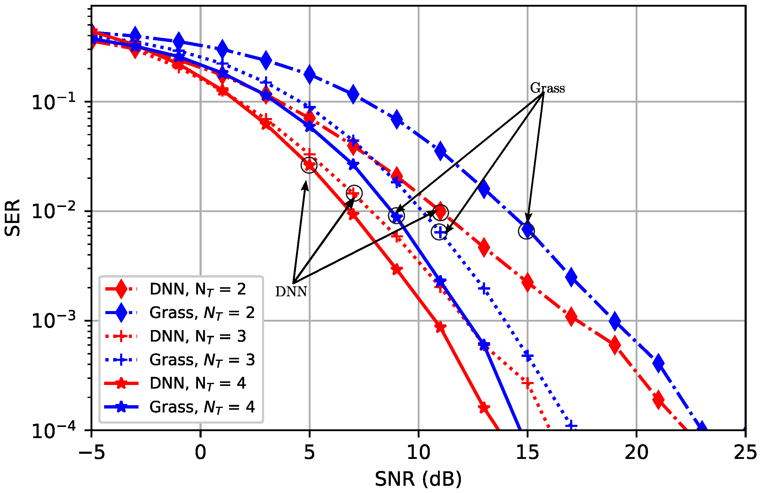
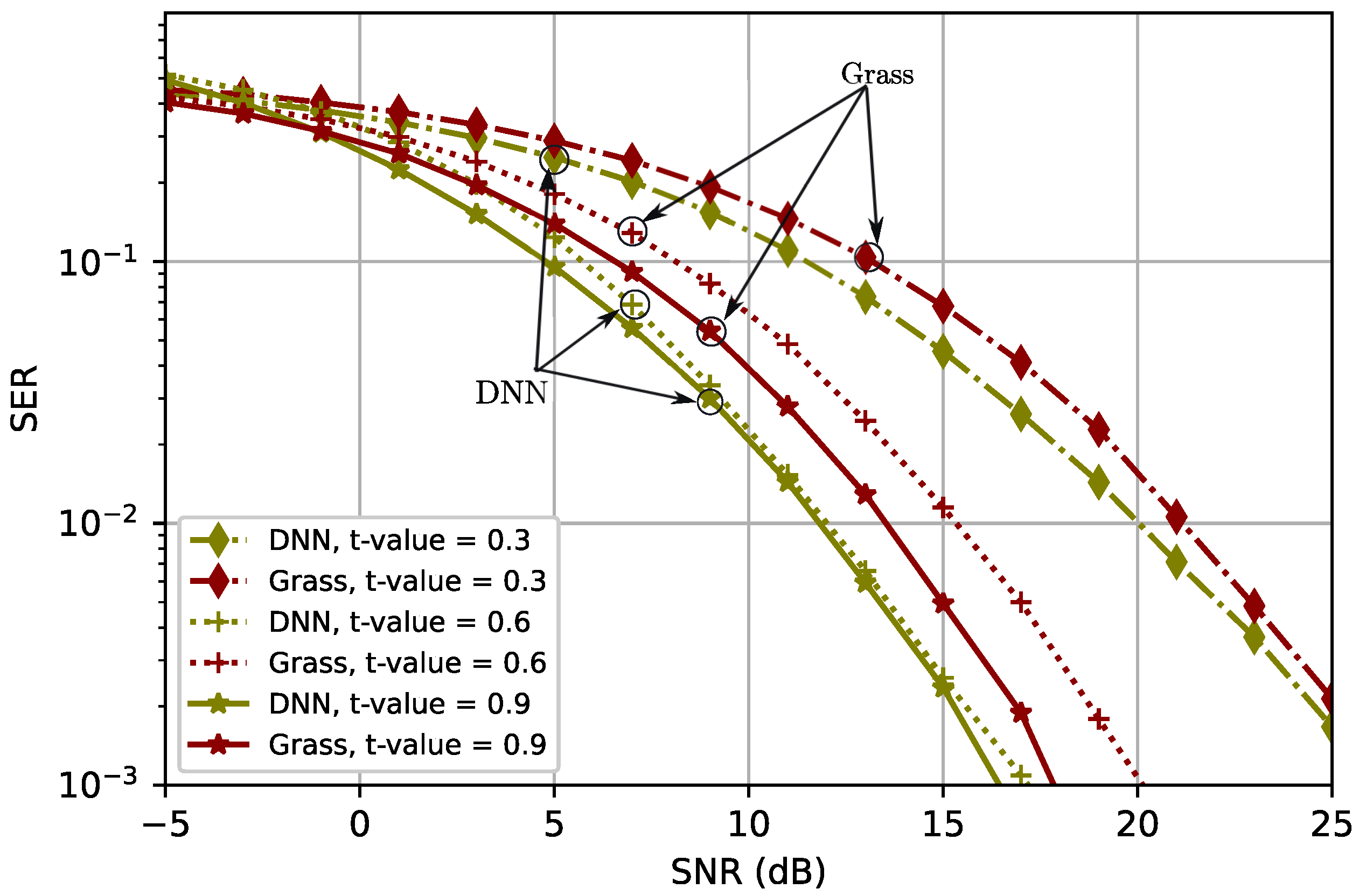
4. Simulation Results

In this section, we analyze the performance of the proposed DNN limited-feedback relay system against a Grassmannian-based codebook system. For our simulation, we have three hidden layers each for the DNNs used for the transmitter, relay, and destination. We perform ${10}^4$ iterations over a batch snap-shot size of $\mathcal{B}=2000$ for our SGD training. For codebook definition, we use a codebook size of 64 with the number of feedback bits (codeword length) set at 6. For simplicity of analysis, we consider a single datastream for the transmissions. We use QPSK as our modulation scheme.

4.1. Grassmannian-Based Benchmark

The Grassmannian codebook (GB) is used in our benchmarking scheme. GB adopts LMMSE for channel estimation, and we assume both to be present at each node. GB serves as a very common codebook choice in terms of its performance. Theoretically, GB outperforms Lloyd-based codebooks. However, the practical implementation of GB presents several challenges due to the difficulties encountered in constructing analytic approaches. Therefore, most designs resort to brute-force searches [24].

Our training dataset is made up of training examples comprising tuples of $\left(\mathbf{H},\mathbf{N}\right)$, from which our ${\mathbf{Y}}^{train}$ is generated. The ${\mathbf{Y}}^{train}$ received signal matrix serves as input to the DNNs. The elements of $\mathbf{H}$ are modeled using a zero-mean complex Gaussian function with covariance ${\mathbf{R}}_{\mathbf{H}}=\mathbb{E}\left[{\mathbf{H}}^H\mathbf{H}\right]$. We use (18) to model the correlation between antennas; the elements of channel matrix $\mathbf{H}$ are indexed as $h_{u,v}$, with u denoting the row and v the column. We evaluate the performance of our proposed DNN limited-feedback system when altering the complex correlation coefficient t [8]:

$${\mathbf{R}}_{\mathbf{H}}=\left\{\begin{array}{cc}{N}_r{t}^{|u-v|}\hfill & \hfill \mathrm{for}u<v,\\ N_r{\left(t^{*}\right)}^{|u-v|}\hfill & \hfill \mathrm{otherwise}.\end{array}\right\}$$

(18)

4.2. Analysis

We analyze the performance of the proposed DNN-based system in terms of the symbol error rate (SER) metric. It is observable that the SER falls with an increase in the number of antennas, with our setup outperforming the GB scheme. In Figure 2, we obtain a performance gap of 1 to 3 dB between the DNN scheme and the GB scheme for antenna configurations of $N_t=N_r=N_d=2\mathrm{and}3$ for the comparative SER values. This is understandable, as the optimization is performed separately, and hence sub-optimally, in the case of the benchmark scheme. Additionally, more information is lost with GB due to its quantization approach. For a finite number of bits accessible in the codebook design structure, there is a limited range of precoders from which selections could be made to characterize the quantized channel. On the other hand, the DNN aggregates a training set when performing its optimization operations, yielding the two beamformers used at the source and destination. This implies that it has access to a greater level of information than the competing scheme. Furthermore, the stochastic gradient descent used in training the DNN results in a more highly refined and optimized gradient vector set over the better information space available to it. Therefore, it is reasonable that the DNN vastly outperforms the GB setup. It is also noteworthy that for lower SNR values of 0 dB to 3 dB, the DNN approach with $N_t=3$ outperforms the Grass-based setup with $N_t=4$ by an average difference of about 1 dB. This suggests that a DNN-based approach with a lower number of antennas could be used to reduce implementation costs in practical applications where there are low power concerns.

It is understood that the DNN approach performs better with an increase in the correlation of the antennas [8]. Thus, for Figure 3, an increase in correlation value—indicated by t-values ($\left|t\right|$) of 0.3, 0.6, and 0.9—reflects increasing levels of performance. These observations again confirm our expectations. Because the benchmarking scheme handles its quantization and limited feedback processes separately, it does not realize the same that are gains achievable from jointly optimizing the problem under consideration. Of great importance here is the sensitivity of the proposed model to variations in the correlation coefficient; whereas a reduction in the correlation results in performance degradation in the Grassmannian approach, the DNN approach responds more sensitively to jumps in correlation (e.g., from 0.6 to 0.3). Nevertheless, it performs better than the benchmark regardless of the correlation level. In addition, the performance benefits become less apparent as the antennas become more highly correlated, at which point more performance can only be extracted from the system by relying on increasing the SNR value.

4.3. Deployment, Practical Considerations, and Limitations

In terms of practical deployment, we envision our system being made operational in a distributed form. Here, the different components of the DNN are placed on graphic processing units (GPUs) or tensor processing units (TPUs) at each node to each instantiate the section of the DNN attributed to them. The limited feedback would then serve the purpose of sending back the most recently updated weights of the preceding node to the next node in the feedback chain. Training could be carried out either offline or online depending on the constraints on the deployed system. For offline systems, designers should consider limitations such as the memory requirements needed for offline training and testing. The parameters obtained after training could then be used for the deployed system. With online training, consideration would have to be given to power limitations if the system is running off the power grid or on a limited power system such as a simultaneous wireless information and power transfer system (SWIPT), as found in [10].

Regardless of the constraints and limitations, our system is more adaptable than traditional codebook-based systems. It can learn from previously unseen instances of CSI as well as node-centric received signals, whether offline or online. The only difference is that the online case takes place in real time, incurring a higher computation cost, whereas the offline case is not real-time, meaning that it has a lower computational cost but will likely be less robust than its online counterpart. It will also require periodic offline retraining for possible updates to its weights and to make improvements. Highlights of the benefits of the different computational complexities are captured in Table 2.

For traditional systems, the feedback overhead comes from the bits sent over to index the beamformer from the codebook, i.e., $i_1^{*}$ and $i_2^{*}$. On the other hand, the corresponding overhead for the DNN-based system comes from the neural-quantized vectors, i.e., ${\mathbf{b}}_D$ and ${\mathbf{b}}_R$. Although the latter system’s overhead cost may be comparatively higher, it is easily offset by the computation benefit of not needing to dereference a codebook at each node for the corresponding beamformer, as well as the practical benefit of generating a beamformed signal that is more suitable to the real-time channel state information (CSI) demands of such a system.

5. Conclusions

This paper has investigated a limited-feedback MIMO relay system using DNN. The DNNs are implemented at each node in the feedback chain. They map the analytic functions that compose our highly nonconvex problem to DNN functions. The performance gap between the DNN scheme and its benchmark increases noticeably with an increase in SNR for each of the performance metrics considered. This indicates that with lower-powered resources, the DNN system can provide similar performance benefits as the predesigned codebooks while considerably outperforming the benchmark at higher SNRs. From our numerical results, the proposed DNN system outperforms the GB scheme in terms of SER serving. Thus, the DNN approach serves as a viable substitute for the codebook approaches.

For future work, our results open up several interesting opportunities in the area of relay-centric DNN-based MIMO systems. The extension of the work to include multiple relays in a cooperative structure or multi-hop setup could offer favorable prospects. In the same vein, a comparison of our system under different modulation schemes could offer further insights. Another route could be the incorporation of reinforcement learning strategies as the learning approach at the different nodes to make the learning process more adaptable to environmental changes. In considering channel estimation and quantization, this work has investigated one-way channel estimation and quantization. Thus, an additional future extension could consider two-way channel estimation based on other machine learning techniques such as generative adversarial networks (cGAN), as discussed in [25].

References

1. Guo, J.; Wen, C.K.; Chen, M.; Jin, S. Environment Knowledge-Aided Massive MIMO Feedback Codebook Enhancement Using Artificial Intelligence. IEEE Trans. Commun. 2022, 70, 4527–4542. [Google Scholar] [CrossRef]
2. Liang, P.; Fan, J.; Shen, W.; Qin, Z.; Li, G.Y. Deep Learning and Compressive Sensing-Based CSI Feedback in FDD Massive MIMO Systems. IEEE Trans. Veh. Technol. 2020, 69, 9217–9222. [Google Scholar] [CrossRef]
3. Zhu, Z.; Yang, R.; Zhang, J.; Xu, S.; Li, C.; Huang, Y.; Yang, L. Sparse Bayesian Learning-Based Adaptive Codebook for Near-Field Channel Estimation. In Proceedings of the ICC 2024—IEEE International Conference on Communications, Denver, CO, USA, 9–13 June 2024; pp. 2366–2371. [Google Scholar] [CrossRef]
4. Yoon, S.G.; Lee, S.J. Improved Hierarchical Codebook-Based Channel Estimation for mmWave Massive MIMO Systems. IEEE Wirel. Commun. Lett. 2022, 11, 2095–2099. [Google Scholar] [CrossRef]
5. Fu, X.; Le Ruyet, D.; Visoz, R.; Ramireddy, V.; Grossmann, M.; Landmann, M.; Quiroga, W. A Tutorial on Downlink Precoder Selection Strategies for 3GPP MIMO Codebooks. IEEE Access 2023, 11, 138897–138922. [Google Scholar] [CrossRef]
6. Mabrouki, S.; Dayoub, I.; Li, Q.; Berbineau, M. Codebook Designs for Millimeter-Wave Communication Systems in Both Low- and High-Mobility: Achievements and Challenges. IEEE Access 2022, 10, 25786–25810. [Google Scholar] [CrossRef]
7. Schwarz, S.; Rupp, M.; Wesemann, S. Grassmannian Product Codebooks for Limited Feedback Massive MIMO with Two-Tier Precoding. IEEE J. Sel. Top. Signal Process. 2019, 13, 1119–1135. [Google Scholar] [CrossRef]
8. Jang, J.; Lee, H.; Hwang, S.; Ren, H.; Lee, I. Deep learning-based limited feedback designs for MIMO systems. IEEE Wirel. Commun. Lett. 2019, 9, 558–561. [Google Scholar] [CrossRef]
9. Ahmed, Y.N.; Fahmy, Y. On the complexity reduction of codebook search in FDD massive MIMO using hierarchical search. In Proceedings of the 2018 International Conference on Innovative Trends in Computer Engineering (ITCE), Aswan, Egypt, 19–21 February 2018; pp. 175–179. [Google Scholar] [CrossRef]
10. Ofori-Amanfo, K.B.; Asiedu, D.K.P.; Ahiadormey, R.K.; Lee, K.J. Multi-Hop MIMO Relaying Based on Simultaneous Wireless Information and Power Transfer. IEEE Access 2021, 9, 144857–144870. [Google Scholar] [CrossRef]
11. Lee, K.J.; Sung, H.; Park, E.; Lee, I. Joint Optimization for One and Two-Way MIMO AF Multiple-Relay Systems. IEEE Trans. Wirel. Commun. 2010, 9, 3671–3681. [Google Scholar] [CrossRef]
12. Song, C.; Lee, K.J.; Lee, I. Performance Analysis of MMSE-Based Amplify and Forward Spatial Multiplexing MIMO Relaying Systems. IEEE Trans. Commun. 2011, 59, 3452–3462. [Google Scholar] [CrossRef]
13. Zhang, Y.; El-Hajjar, M.; Yang, L.L. Adaptive Codebook-Based Channel Estimation in OFDM-Aided Hybrid Beamforming mmWave Systems. IEEE Open J. Commun. Soc. 2022, 3, 1553–1562. [Google Scholar] [CrossRef]
14. Wen, C.K.; Shih, W.T.; Jin, S. Deep learning for massive MIMO CSI feedback. IEEE Wirel. Commun. Lett. 2018, 7, 748–751. [Google Scholar] [CrossRef]
15. Brilhante, D.d.S.; Manjarres, J.C.; Moreira, R.; de Oliveira Veiga, L.; de Rezende, J.F.; Müller, F.; Klautau, A.; Leonel Mendes, L.; de Figueiredo, F.A.P. A literature survey on AI-aided beamforming and beam management for 5G and 6G systems. Sensors 2023, 23, 4359. [Google Scholar] [CrossRef] [PubMed]
16. Nada, A.E.R.; Mehana, A.M.H. A Comparative Study of PMI/RI Selection Schemes for LTE/LTEA Systems. IEEE Trans. Veh. Technol. 2018, 67, 1444–1453. [Google Scholar] [CrossRef]
17. Zhang, M.; Shafi, M.; Smith, P.J.; Dmochowski, P.A. Precoding Performance with Codebook Feedback in a MIMO-OFDM System. In Proceedings of the 2011 IEEE International Conference on Communications (ICC), Kyoto, Japan, 5–9 June 2011; pp. 1–6. [Google Scholar] [CrossRef]
18. Asiedu, D.K.P.; Lee, H.; Lee, K.J. Simultaneous Wireless Information and Power Transfer for Decode-and-Forward Multihop Relay Systems in Energy-Constrained IoT Networks. IEEE Internet Things J. 2019, 6, 9413–9426. [Google Scholar] [CrossRef]
19. Laue, H.E.A.; du Plessis, W.P. A Coherence-Based Algorithm for Optimizing Rank-1 Grassmannian Codebooks. IEEE Signal Process. Lett. 2017, 24, 823–827. [Google Scholar] [CrossRef]
20. Schwarz, S.; Tsiftsis, T. Codebook Training for Trellis-Based Hierarchical Grassmannian Classification. IEEE Wirel. Commun. Lett. 2022, 11, 636–640. [Google Scholar] [CrossRef]
21. Li, S.; Jia, H.; Kang, J. Robust Codebook Design Based on Unitary Rotation of Grassmannian Codebook. In Proceedings of the 2010 IEEE 72nd Vehicular Technology Conference—Fall, Ottawa, ON, Canada, 6–9 September 2010. [Google Scholar] [CrossRef]
22. Lim, S.; Shin, M.; Paik, J. Point Cloud Generation Using Deep Adversarial Local Features for Augmented and Mixed Reality Contents. IEEE Trans. Consum. Electron. 2022, 68, 69–76. [Google Scholar] [CrossRef]
23. Melgar, A.; de la Fuente, A.; Carro-Calvo, L.; Barquero-Pérez, Ó.; Morgado, E. Deep Neural Network: An Alternative to Traditional Channel Estimators in Massive MIMO Systems. IEEE Trans. Cogn. Commun. Netw. 2022, 8, 657–671. [Google Scholar] [CrossRef]
24. Villardi, G.P.; Ishizu, K.; Kojima, F. Reducing the Codeword Search Complexity of FDD Moderately Large MIMO Beamforming Systems. IEEE Trans. Commun. 2019, 67, 273–287. [Google Scholar] [CrossRef]
25. Baek, S.; Moon, J.; Park, J.; Song, C.; Lee, I. Real-Time Machine Learning Methods for Two-Way End-to-End Wireless Communication Systems. IEEE Internet Things J. 2022, 9, 22983–22992. [Google Scholar] [CrossRef]
Figure 1. DNN-based relay-aided limited-feedback design and signal flow.
Mathematics 13 02246 g001
Figure 2. SER vs. varying SNR for different number of antennas = { 2 , 3 , 4 } .
Mathematics 13 02246 g002
Figure 3. SER vs. varying SNR for different t-values | t | = { 0.3 , 0.6 , 0.9 } .
Mathematics 13 02246 g003